Magnetic field oscillations of the critical current in long ballistic graphene Josephson junctions

Abstract

We study the Josephson current in long ballistic superconductor-monolayer graphene-superconductor junctions. As a first step, we have developed an efficient computational approach to calculate the Josephson current in tight-binding systems. This approach can be particularly useful in the long junction limit, which has hitherto attracted less theoretical interest but has recently become experimentally relevant. We use this computational approach to study the dependence of the critical current on the junction geometry, doping level, and an applied perpendicular magnetic field $B$. In zero magnetic field we find a good qualitative agreement with the recent experiment of Ben Shalom et al. (Reference graphene_Falko, ) for the length dependence of the critical current. For highly doped samples our numerical calculations show a broad agreement with the results of the quasiclassical formalism. In this case the critical current exhibits Fraunhofer-like oscillations as a function of $B$. However, for lower doping levels, where the cyclotron orbit becomes comparable to the characteristic geometrical length scales of the system, deviations from the results of the quasiclassical formalism appear. We argue that due to the exceptional tunability and long mean free path of graphene systems a new regime can be explored where geometrical and dynamical effects are equally important to understand the magnetic field dependence of the critical current.

I Introduction

The recent progress in the fabrication techniques of graphene devices allows to obtain exceptionally high mobilities with mean free paths of several $\mu$ms in graphene devices crdean2010 ; mayorov ; crdean2013 . Thus a new field has opened for experiments, the electron optics of two-dimensional Dirac electrons marcus ; schonenberger2013 ; schonenberger2015 ; ozyilmaz ; hu-jong . Very recently, several work has made a further exciting step by contacting such high-quality graphene samples with superconducting electrodes xudu2013 ; vandersypen ; yacobi2015a ; graphene_Falko ; xudu2015 ; specular-andreev and observed a finite Josephson current flowing over $\mu$m distances vandersypen ; graphene_Falko . In addition, the interface between the superconducting (S) and graphene (G) regions was found to be significantly more transparent than in previous experiments xudu2013 ; morpurgo2007 ; lau2007 ; bouchiat2007 ; andrei ; siddiqi ; bouchiat2009 ; leehj2011a ; leehj2011b ; bezryadin ; schonenberger2012 ; gueron ; leehj2013 ; esquinazi . These experimental advances may allow to verify some of the theoretical predictions for graphene-superconductor heterostructures, such as anharmonic phase-current relation of supercurrent at low temperatures in superconductor-graphene-superconductor (SGS) junctions in monolayer black-schaffer2008 ; black-schaffer2010 ; hagymasi ; peeters2012 and bilayer peeters2012 ; moghaddam graphene, supercurrent quantization in quantum point contacts zareyan2006 ; zareyan2007 , specular Andreev reflection beenakker2006 ; qing-feng2009 ; qing-feng2011 ; recher , detection of valley polarization beenakker2007 , interplay of strain and superconductivity peeters2011 ; linder ; bwang etc. in the near future.

The theoretical work has mainly focused on short SGS junctions to date moghaddam ; zareyan2006 ; zareyan2007 ; linder ; Carlo_short1 ; imura , where the length of the normal region $L$ is smaller than the superconducting coherence length $\xi_{0}=\frac{\hbar v_{F}}{\Delta_{0}}$. In addition, it was usually assumed that the width $W$ of the junction is much larger than $L$. Although the long junction regime has been studied theoretically for superconductor-normal metal-superconductor (SNS) systems ishii ; bardeen ; bratus1972 ; miller ; diffusive_long_SNS ; bergeret ; cuevas , the physics of long SGS junctions is less explored. An experimental study of long ($L\gtrsim\xi_{0}$) and wide ($W\gg L$) diffusive SGS junctions was presented in Reference gueron, . However, in recent experiments different transport regimes have become accessible, where ballistic propagation was achieved in graphene samples where $L\gtrsim\xi_{0}$ vandersypen ; graphene_Falko and/or $W/L\approx 1$vandersypen . Furthermore, the dependence of the superconducting critical current $I_{c}$ on a perpendicular magnetic field ${B}$ has also been measuredvandersypen ; yacobi2015a ; graphene_Falko in these SGS junctions. While References yacobi2015a ; graphene_Falko have found that the oscillations of $I_{c}$ as a function of ${B}$ can be described, at least in doped samples, by a Fraunhofer-like interference pattern, in Reference vandersypen deviations from the Fraunhofer pattern have been observed for samples that are in the long junction limit and have an aspect ratio $W/L\approx 1$. Previously, deviations from the Fraunhofer-like $I_{c}({B})$ dependence were also observed in SNS junctions both in the diffusive bouchiat2012 and in the quasi-ballistic limit anomalous_osc1 , and the subsequent theoretical work have elucidated the role of the junction geometry blatter ; zagoskin1999 ; zagoskin2003 using the quasiclassical Green’s function approach. It is not immediately clear, however, if these theoretical results are directly applicable to SGS junctions, especially in the low doping regime.

Our aim in this work is twofold. Firstly, we want to present a newly developed computational approach to calculate the Josephson current in tight-binding (TB) systems. The method is general and can be implemented for many TB systems, not only for graphene. It takes into account on equal footing the contributions coming from both the Andreev bound states (ABS) and the scattering states (ScS), the latter being especially important in long Josephson junctions, where it is known that cancellation between different supercurrent contributions occur bratus1972 ; affleck2013 . Since our method accounts for both contributions, it can be used for efficient simulations of recent experimental systems vandersypen ; yacobi2015a ; graphene_Falko . Secondly, using the above computational method, we study the length $L$ and magnetic field dependence of the critical current in long SGS junctions. Although the length dependence of $I_{c}$ has been studied before using various theoretical approaches black-schaffer2008 ; hagymasi ; perfetto ; jafari we revisit this question because the recent observations in Reference graphene_Falko offer the possibility to directly compare theory and experiments. Encouragingly, we find a good qualitative agreement between our results and the experimental observations of Reference graphene_Falko , indicating that our approach can capture important aspects of the physics of long SGS junctions. Regarding the magnetic field effects in long SGS junctions, to our knowledge no detailed study is available at present. We study the magnetic field oscillations of $I_{c}$ as function of the doping of the normal region. For high doping we find that the semiclassical formalism blatter ; zagoskin1999 ; zagoskin2003 , developed for ballistic Josephson junction where the normal region is a two-dimensional electron gas, can also describe the oscillations $I_{c}$ in SGS junctions. However, for lower doping, where the cyclotron radius $R_{c}$ becomes comparable to $W$ and/or $L$, orbital effects can no longer be neglected and deviations from the quasiclassical results appear.

The paper is organized as follows. In Section II we briefly introduce the model system that we used in our calculations. In order to make the paper accessible to a broad audience, this is followed by the presentation of our main results for the critical current $I_{c}$. First, in Section III we discuss the length dependence of $I_{c}$ and also the current-phase relation. The effect of the magnetic field on $I_{c}$ is treated in Section IV. A general numerical approach to calculate the Josephson current for TB Hamiltonians is presented in Section V, while some of the relevant details of the TB model used in this work is given in Section VI. Finally, we conclude with Section VII.

II The model

We first briefly describe the model we employed to calculate the Josephson current in SGS junctions, further details can be found in Section VI. In the normal conducting region of length $L$ and width $W$ we use the nearest-neighbour TB model of graphene wakabayashi ; graphene-review with the Hamiltonian

$$\hat{H}=\sum_{i}\varepsilon_{i}c_{i}^{\dagger}c_{i}-\sum_{\langle ij\rangle}\gamma_{ij}c_{i}^{\dagger}c_{j}+h.c.$$ (1)

Here $\varepsilon_{i}$ is the on-site energy on the atomic site $i$, $\gamma_{ij}$ is the hopping amplitude between the nearest neighbour atomic sites $\langle ij\rangle$ in the graphene lattice, and $c_{i}^{\dagger}$ ($c_{i}$) creates (annihilates) an electron at site $i$. The magnetic field can be incorporated by means of the Peierls substitution peierls :

$$\gamma_{ij}=\gamma\;{\rm Exp}\left(\frac{2\pi{\rm i}}{\phi_{0}}\int\limits_{\mathbf{R}_{j}}^{\mathbf{R}_{i}}\mathbf{A(\mathbf{r})}{\rm d}\mathbf{r}\right),$$ (2)

where $\phi_{0}=h/e$ is the flux quantum, $\mathbf{A}(\mathbf{r})$ denotes the vector potential and the vector $\mathbf{R}_{i}$ points to the $i$th atomic site in the lattice. The spatial dependence of $\mathbf{A}(\mathbf{r})$ is such that it yields a homogeneous perpendicular magnetic field $\mathbf{B}=(0,0,B_{z})^{T}$ in the normal region and zero field in the superconducting regions, see Section VI.3.

The superconducting regions are modelled by a highly doped graphene regionCarlo_short1 of width $W$ and open boundary condition in the transport direction. It is assumed that a finite on-site pair-potential $\Delta_{0}e^{i\varphi_{L,R}}$ is induced by proximity effect in the left (L) and right (R) electrodes. We note that our methodology would allow for other models of the superconducting regions as well martin-rodero . For the superconducting pair-potential we assume a step-like change at the normal-superconductor (NS) interfaces:

$$\Delta(x)=\left\{\begin{array}[]{ll}\Delta_{0}e^{{\rm i}\varphi_{L}}&\textrm{if }x<0\\ 0&\textrm{if }0\leq x\leq L\\ \Delta_{0}e^{{\rm i}\varphi_{R}}&\textrm{if }x>L\end{array}\right..$$ (3)

Here $\varphi_{L}$ ($\varphi_{R}$) is the phase of the pair-potential in the left (right) lead and we will denote by $\delta\varphi=\varphi_{R}-\varphi_{L}$ the phase difference. Our main interest in this work is to study SGS junctions where there is a significant difference between the doping levels of the S and N regions: $\lambda_{S}\ll\lambda_{N}$ where $\lambda_{S(N)}$ is the Fermi wavelength in the superconductor (normal) region. Moreover, the junction is long $L/\xi_{0}\gtrsim 1$ with respect to the coherence length $\xi_{0}$. In this case we expect that the detailed spatial dependence of $\Delta_{0}$ in the vicinity of the normal-superconductor interface is not very important and therefore the above approximation should give qualitatively correct results. Indeed, References black-schaffer2008 ; black-schaffer2010 ; peeters2012 ; peeters2013 ; alidoust have shown that the self-consistent calculation of $\Delta(x)$ in clean SGS junctions is most important for (i) short junctions, (ii) no Fermi-level mismatch between the S and N regions, (iii) temperatures close to $T_{c}$.

The simulation of realistic samples on the micrometer length scale is quite challenging in the TB framework due to the huge number of the atomic sites. Part of the problem can be circumvent by using an efficient numerical approach, see Section VI.1 for details. Moreover, we expect that experimentally relevant informations can be extracted from TB systems that follow certain scaling laws but imply significantly lower computational costs. Such an approach has proved to be very useful recently in the calculation of normal transport graphene_antidot_sajat ; TB_scaling for mesoscopic graphene structures. We expect that as long as the characteristic dimensions $W$ and $L$ of the system are much larger than the lattice constant of graphene, the same physical behavior should be observed in systems with the same $L/\xi_{0}$, $W/L$, $\frac{2W}{\lambda_{N}}$, $\frac{\xi_{0}}{\lambda_{N}}$, $\frac{T}{T_{c}}$ and $L/l_{B}$ control parameters, where $\lambda_{N}=\frac{E_{F}}{\hbar v_{F}}$ is the Fermi wave number in the normal region $l_{B}=\frac{\hbar}{|eB|}$ is the magnetic length and $T_{c}\approx\Delta_{0}/(1.76k_{B})$ is the critical temperature. We are interested here in the bulk properties of the supercurrent, i.e., we need to ensure that edge effects do not play role. In most of our calculations we used zigzag nanoribbons, however, we have checked that we obtain very similar results for armchair nanoribbon as well. (see Section III). Therefore we expect that our results would not change for more general edges either.

III Zero magnetic field results

III.1 Length dependence of $I_{c}$

An important property of long Josephson junctions is the dependence of the critical current $I_{c}$ on the junction length $L$, which was measured recently in Reference graphene_Falko . In general, at zero temperature $I_{c}$ is given by the relationCarlo_revmod

$$I_{c}=\alpha\frac{e|\Delta_{0}|}{\hbar}N,$$ (4)

where $N$ is the number of open channels in the normal region: $N=\frac{E_{F}W}{\pi\hbar v_{F}}=\frac{Wk_{F}}{\pi}=\frac{2W}{\lambda_{F}}.$ The dimensionless coefficient $\alpha$ can depend on a number of factors, such as the junction transparency, the presence of a $p-n$ junction or other disorder induced by the superconducting contacts, the doping level in the normal region Carlo_short1 etc. However, for the case considered here (no disorder at the SG interface) and in the long junction limit $\alpha$ is expected to be a function of the ratio $L/\xi_{0}$ only bardeen ; bratus1972 .

Figure 1: Length dependence of $I_{c}$ for different temperatures $T/T_{c}$. Different symbols correspond to calculations performed with zigzag ribbons of different width: $W=149\,{\rm r}_{cc}$ ($\vartriangle$), $W=299\,{\rm r}_{cc}$ ($\triangledown$), and $W=449\,{\rm r}_{cc}$ ($\circ$), where ${\rm r}_{cc}$ is the carbon-carbon bond length. The calculations shown with $\square$ were obtained for an armchair nanoribbon of width $W=301\,{\rm r}_{cc}$. Solid lines show the results of fitting, the obtained fit parameters are indicated in each figures. The chemical potential in graphene is $\mu_{N}=80\Delta$.

First, in Figure 1(a) we present the zero temperature calculations for $\alpha$. The good agreement between the calculations for different widths and edge types indicates that these results are free of finite size and edge effects. One can see that the numerical results can be fitted with a function $A/(L/\xi_{0}+C)$, where $A$ and $C$ are fitting parameters. For $L/\xi_{0}\gg C$ the critical current falls off as $1/L$, whereas in the short junction limit $L/\xi_{0}\ll 1$ it goes to a finite value and reproduce the analytical prediction of Reference Carlo_short1, : for $L/\xi_{0}\rightarrow 0$ and $\lambda_{S}\ll\lambda_{N}$ the value of $\alpha$ is $\approx 1.22$. Next, in Figures 1(b)-(d) we show the $I_{c}(L)$ curves for low, but finite temperatures $T$. As the temperature is increased from $T=0$, both fit parameters $A$ and $C$ decrease and eventually there is a temperature range where the parameter $C$ becomes very small so that $I_{c}$ falls off as $\sim 1/L$ for $L/\xi_{0}\gtrsim 1.0$ [Figures 1(b)-(c)]. Such a $\sim 1/L$ dependence of $I_{c}$ was recently observed in Reference graphene_Falko . It was suggested that this peculiar $I_{c}(L)$ dependence is a signature of the SGS junctions being truly ballistic and in the long junction limit. Our calculations support this conclusion, nevertheless, it would be interesting to measure $I_{c}(L)$ at lower temperatures in order to map out experimentally the $T$ dependence of the parameters $A(T)$ and $C(T)$ and compare it to our results. It is important to note the following: (i) Taking the $T_{c}$ of bulk niobium, the experimental data of Reference graphene_Falko, correspond to $T/T_{c}=0.045$, i.e., to lower temperature than shown in Figure 1(b). However, if one assumes that the induced pair potential in the graphene is smaller than the bulk value of $\Delta$, i.e., it corresponds to a smaller $T_{c}$, then the agreement with our calculations becomes better. (ii) The values of $\alpha$ in Figure 1(c) significantly overestimate the experimental ones reported in Reference graphene_Falko, . We think this is due to the fact that we have assumed perfectly transparent SG interface and no disorder in the normal part of the junction, while in Reference graphene_Falko, the SG interface had a finite transparency and a p-n junction was probably formed due to the doping effect of the contacts. We leave the study of these effects for a future work. Finally, as shown in Figures 1(d), as the temperature is further increased such that the energy scale $k_{B}T$ becomes non-negligible with respect to the ballistic Thouless energy $\frac{\hbar v_{F}}{L}$ bardeen ; miller , $I_{c}$ becomes exponentially suppressed: $I_{c}\sim e^{-cL/\xi_{0}}$, where $c$ is a fitting parameter.

III.2 Current-phase relation

Regarding the current-phase relation (CPR), it has long been known that the CPR in long SNS Josephson junctions ishii ; bardeen ; bratus1972 is substantially different from the $\propto\sin(\delta\phi)$ relation valid in the short junction limit Kulik_shortSNS . In the one-dimensional TB model studied in Reference cini, the deviation from the $\propto\sin(\delta\phi)$ dependence was explained by the contribution of the scattering states to the total current which becomes comparable to the contribution of the Andreev bound states as the length of the junction increases. A partial cancellation effect between the different contributions to the Josephson current in SNS junctions was also pointed out by References bardeen, ; bratus1972, . Recently, anharmonic CPR was found in the calculations of References black-schaffer2008 ; black-schaffer2010 ; peeters2012 for SGS junctions. We have also calculated the CPR using our method for a long SGS junction. As one can see in Figure 2(a), at zero temperature the CPR deviates significantly from the $\propto\sin(\delta\phi)$ dependence and for $\delta\phi/\pi\lesssim 0.3$ it is a linear function of $\delta\phi/\pi$.

Figure 2: The Josephson current as a function of the phase difference $\delta\phi=\phi_{R}-\phi_{L}$ between the superconducting electrodes (in units of $e\Delta_{0}/\hbar$). The parameters are $\mu_{N}=32\Delta_{0}$, $W/L=1.15$, and $L/\xi_{0}=1.48$. The total current is denoted by solid lines, and the separate contributions of the scattering states (dashed-dotted) and of the Andreev bound states (dash-dotted) are also shown. Black lines show the results obtained using zigzag nanoribbons, green lines indicate armchair results. The ribbon width was $W=300\,{\rm r}_{cc}$.

The contribution coming from the ScS (dashed-dotted line) is of the same magnitude as the contribution of the ABSs (dashed line). In Figure 2(a) the two contributions have the same sign, however, this is not always the case: calculations not shown here indicate that depending on the $L/\xi_{0}$ ratio the supercurrent due to the ScS can be either positive or negative. For finite temperatures [see Figure 2(b)], similarly to SNS junctions bardeen , the CPR acquires a harmonic dependence on $\delta\phi$. In these wide ribbons the major characteristics of the CPR do not depend on whether zigzag or armchair nanoribbons are used in the calculations.

To briefly summarize the results presented in this section, we find that our results show a good qualitative agreement with i) the measurements of Reference graphene_Falko, for the length dependence of $I_{c}$, ii) with previous theoretical works black-schaffer2010 ; peeters2012 for the CPR, even though we do not calculate the pair potential $\Delta$ self-consistently. This suggests that in long SGS JJs, if there is a finite Fermi-level mismatch at the SG interface, the self-consistent calculation of $\Delta$ is less important than in the short junction limit with no Fermi-level mismatch.

IV Oscillations of the critical current in perpendicular magnetic field

We now turn to the properties of the critical current in the presence of a perpendicular magnetic field $B$. Oscillations of $I_{c}$ have been measured in several recent experiments vandersypen ; yacobi2015a ; graphene_Falko but have not yet received much theoretical attention. It is well known that in tunnel junctions $I_{c}$ exhibits Fraunhofer-like oscillations as a function of the piercing magnetic flux $\Phi$ with a period $\phi_{0}=h/2e$ and oscillation minima at integer multiples of the flux quantum $\phi_{0}$: $I_{c}(B)=I_{c}(0)\left|\frac{{\rm sin}(\pi\Phi/\phi_{0})}{\pi\Phi/\phi_{0}}\right|,$ where $I_{c}(0)$ is the zero-field critical current. The long junction limit in SNS systems was studied in References blatter ; zagoskin1999 ; zagoskin2003 ; svidzinskii using the quasiclassical Green’s function formalism. It was pointed out that the magnetic field oscillation of $I_{c}$ also depend on the geometry of the junctions. For wide and long ballistic junctions, where $W\gg L\gg\xi_{0}$, the critical current oscillates as zagoskin1999 ; svidzinskii

$$I_{c}(B)=I_{c}(0)\frac{(1-\{\Phi/\phi_{0}\})\{\Phi/\phi_{0}\}}{|\Phi/\phi_{0}|},$$ (5)

$\{x\}$ denoting the fractional part of $x$. The oscillation pattern given by Eq. (5) is very similar to the Fraunhofer-like oscillations in tunnel junctions, except for $\Phi/\phi_{0}\ll 1$. However, deviations from Eq. (5) were observed in the measurements of Reference anomalous_osc1, in quasi-ballistic SNS junctions. Subsequent theoretical work blatter ; zagoskin1999 showed that geometrical effects become important when $W\sim L\gg\xi_{0}$. In particular, Reference blatter, found that the periodicity of $I_{c}$ as a function of magnetic field changes from $\phi_{0}$ [see Eq. 5] to $2\phi_{0}$ as the flux through the junction increases and at low temperatures the crossover to the $2\phi_{0}$ periodicity appears at a flux $\sim\phi_{0}W/L$. Regarding the recent experiments in SGS junctions, Fraunhofer-like pattern for $I_{c}(B)$ was found in Reference graphene_Falko, for wide ($W\gg L$) junctions, whereas Reference vandersypen, measured periodicity that was longer than $\phi_{0}$ for junctions with aspect ratios $W/L\approx 1$.

An important assumption behind the quasiclassical formalism blatter ; zagoskin1999 ; zagoskin2003 ; svidzinskii is that the effect of magnetic field can be taken into account through a phase factor that the wave function of the quasiparticles acquires along classical trajectories that are straight lines. This is a good approximation when the cyclotron radius of the particles is much larger than other characteristic length scales in the system.

However, compared to traditional SNS systems, the exceptional tunability of the state-of-the-art graphene systems, combined with the use of Nb graphene_Falko or MoRe vandersypen superconductors allows, in principle, to reach a regime where the size of the cyclotron radius $R_{c}$ is comparable to $W$ and/or $L$ already for relatively low magnetic fields such that the effect of magnetic field on the superconducting electrodes can still be neglected. Considering the semiclassical cyclotron radius $R_{c}$ in graphene $R_{c}=\frac{E_{F}l_{B}^{2}}{\hbar v_{F}}$ one can see that for a charge density $n_{e}\approx 10^{12}\frac{1}{cm^{2}}$ the cyclotron radius is $\approx 1\mu$m for a $B\approx 0.1T$. Thus $R_{c}$ becomes an important length scale when the chemical potential approaches the charge neutrality point. This regime is expected to harbour rich physics, because geometrical effects, discussed above, and dynamical effects related to the curved semiclassical trajectories of the quasiparticles are equally important. It is then not clear if the quasiclassical formalism blatter ; zagoskin1999 ; svidzinskii , which neglects the dynamical effects, can still give a good description. The possible importance of this regime has also been discussed in Reference graphene_Falko, .

In the following we take the chemical potential $\mu_{N}$ in the normal region as a tuning parameter discuss separately the high doping limit, when $R_{c}\gg L,W$ holds for the considered magnetic field range, and the low doping range, where $R_{c}\gtrsim L,W$ can be reached for relatively small magnetic fields. In all our calculations we assume that the effect of magnetic field on the pair potential in the superconducting contacts can be neglected.

IV.1 High doping limit

To see if the quasiclassical theory blatter ; zagoskin1999 also applies to SGS junctions when the normal region is strongly doped, we calculate $I_{c}(B)$ for different $W/L$ ratios. We have found that the oscillations depend only weakly on the exact value of $L/\xi_{0}$ and on the temperature (in the low temperature limit relevant for recent experiments vandersypen ; yacobi2015a ; graphene_Falko ). Thus, we present our results only for particular temperature and $L/\xi_{0}$ values. Figure 3 shows the magnetic oscillations calculated for different aspect ratios $W/L$ calcs-detail . These results were obtained for zigzag nanoribbons but we have checked that the results do not change qualitatively for armchair nanoribbons. For wide junctions [Figure  3(a)], we recover the Fraunhofer-like pattern of the oscillations with minimums at integer multiples of the flux quantum $\phi_{0}$, see Eq. (5). Deviations from the ideal curve Eq. (5) start to appear only for magnetic fluxes $\Phi\gtrsim 4\phi_{0}$.

Figure 3: The normalized critical current as a function of the magnetic flux piercing the SGS junction (circles). In all figures $L/\xi_{0}=1.63$, and the temperature was $T/T_{c}=0.013$. In (c) the vertical dashed lines show the position of the current minima. The distance between the minima is $1.1\phi_{0}$ in the plotted magnetic field range. The solid (red) line represents the standard Fraunhofer-like oscillation pattern given by Eq. (5).

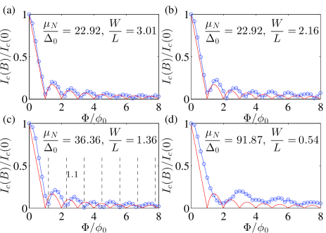
As the aspect ratio $W/L$ decreases [Figures 3(b)-(c)], the periodicity of $I_{c}$ becomes longer than $\phi_{0}$, even for smaller magnetic fields. Interestingly, for $W/L\sim 1$ [Figure 3(c)] the oscillation period is roughly constant in the considered magnetic field range. Finally, in Figure 3(d) one can see that in narrow samples the first minimum in $I_{c}$ is at $2\phi_{0}$ and the current does not go to zero. These results are in broad agreement with the quasiclassical calculations of Reference blatter, indicating that $I_{c}(B)$ in highly doped graphene samples can essentially be described by the theory used previously for SNS junctions in References blatter, ; zagoskin1999, ; svidzinskii, . As mentioned above, deviations from the Fraunhofer-like pattern, similar to the ones shown in Figures 3(c) and (d) have been measured recently in Reference vandersypen, for samples with $W/L\approx 1$. However, a more quantitative comparison of our calculations with Reference vandersypen, is difficult because i) due to the inevitable disorder at the edges, the effective width of the samples may be smaller than the geometrical width, and ii) the current oscillations are likely to depend on the properties of the $p$-$n$ junction formed at the SG interface which is not taken into account in our calculations.

IV.2 Low doping limit

We now consider the case when the doping of the normal region approaches the charge neutrality point, but it is still large enough so that the formation electron-hole puddles can be neglected. The most interesting results in this parameter range are shown in Figure 4. As in the high doping case, the current oscillations depend on the aspect ratio $W/L$. For wide junctions, as in Figure 4(a), the oscillations are similar to the strong doping case shown in Figure 3(a) but the oscillation period is somewhat longer and the amplitude, relative to $I_{c}(0)$, is larger. For $L>R_{c}$, however, the current is strongly suppressed. In Figures 4(b)-(d) we calculate the current for a narrower junction as the doping is decreased. Comparing Figure 4(b) and Figure 3(c), where the same geometrical parameters were used, one can see that for smaller doping dynamical effects influence the period of the current oscillations. (As indicated in Figure 4(b), the ratio $L/R_{c}\approx 1$ is obtained for $\Phi/\phi_{0}\approx 7.8$ in this case. ) While in the strongly doped case [Figure 3(c)] the period of oscillations is $\approx 1.1\phi_{0}$ in the shown magnetic field range, for smaller doping the distance between consecutive minima grows with the magnetic field. As the doping level is further reduced the oscillations of $I_{c}$ become rather complex for magnetic fields where $L>R_{c}$ is fulfilled, see Figures 4(c) and (d). The regime $\Phi/\phi_{0}\gtrsim 5.8$ [$\Phi/\phi_{0}\gtrsim 3.8$] in Figure 4(c) [Figure 4(d)] illustrates that geometrical effects (due to $W\sim L$) and dynamical effects ($R_{c}\sim L$) can both strongly affect the oscillation pattern. Note, that for the parameters used in Figure 4(b)-(d) the diameter of the cyclotron motion is still smaller than the geometrical parameters, i.e., $2R_{c}>W,L$ and therefore no quantum Hall edge states are formed.

Figure 4: The normalized critical current as a function of the magnetic flux piercing the SGS junction. The parameters used in these calculations were $L/\xi_{0}=1.63$, and $T/T_{c}=0.013$. The solid (red) line represents the standard Fraunhofer-like oscillation pattern given by Eq. (5). The dashed vertical lines in panel (b) indicate the minima of the current. Vertical arrows indicate the $\Phi/\phi_{0}$ values where the cyclotron radius equals the length of the junction, i.e., $R_{c}=L$.

The regime $R_{c}\gtrsim L$ has recently been considered in Reference graphene_Falko, , where the sample dimensions were $W\gg L\gtrsim\xi_{0}$. The suppression of the supercurrent was discussed in terms of the constraints that classical trajectories, corresponding to electron-hole pairs, have to fulfill in order that Cooper-pairs can be transferred between the superconductors. It was argued, amongst other, that electron-hole trajectories should not drift farther away than the size of Cooper-pair wave packet in the superconductor. For wide junctions [Figure 4(a)], our results seem to be in qualitative agreement with the semiclassical picture put forward in Reference graphene_Falko, . For junctions where $W\sim L\sim\xi_{0}$ [Figures 4(b)-(d)], the situation is somewhat different from the wide junction case because here the electron-hole trajectories cannot drift away to large distances and are more likely to form (nearly) closed orbits and hence bound states. This may explain why the supercurrent is not suppressed.

V Tight-binding approach to calculate the DC Josephson current

In this section we describe the TB approach we used to calculate the DC Josephson current. It is a generalization of the approach developed to calculate two-terminal normal transport sanvito1999 ; smeagol-paper to the case when both terminals are superconducting and the main interest is not the scattering matrix (and the differential conductance) but the current flowing due to the superconducting phase difference between the terminals. As already mentioned, the method is general and can be implemented for many TB system. It is a generalization of the one-dimensional TB work by References cini, ; cbena, to nanoribbon geometries and would also allow for extension to multi-terminal systems studied, e.g., in References qing-feng2009, ; qing-feng2011, ; akhmerov2014, . The actual calculations presented in Sections III and IV were performed with the EQuUs software equus .

V.1 The general setup

The studied system, including the central region and the electrodes, is schematically depicted in Fig. 5.

Figure 5: The atomic sites are grouped into a sequence of slabs that are connected by nearest neighbour couplings. The central region is formed by the slabs from $1$ to $N$, while the slabs $0$ and $N+1$ are the surface slabs of the left and right electrodes connected to the normal region.

The atomic sites of the system are arranged into slabs that are coupled to each other by nearest neighbour coupling matrices $H_{1}^{i,i+1}$ and $H_{-1}^{i+1,i}$. The $i$th slab contains of $N_{i}$ sites and is described by a Hamiltonian $H_{0}^{i}$. The central (scattering) region is formed by the slabs from $1$ to $N$, while the slabs $0$ and $N+1$ are the surface slabs of the infinite left and right (superconducting) electrodes. Thus, the Hamiltonian of the infinite system can be organized in the following block-diagonal form:

$$\hat{H}=\left(\begin{array}[]{cccccc}\dots&\dots&\dots&\dots&\dots&\dots\\ \dots&H_{0}^{i-1}&H_{1}^{i-1,i}&0&0&\dots\\ \dots&H_{-1}^{i,i-1}&H_{0}^{i}&H_{1}^{i,i+1}&0&\dots\\ \dots&0&H_{-1}^{i+1,i}&H_{0}^{i+1}&H_{1}^{i+1,i+2}&\dots\\ \dots&0&0&H_{-1}^{i+2,i+1}&H_{0}^{i+2}&\dots\\ \dots&\dots&\dots&\dots&\dots&\dots\end{array}\right)$$ (6)

Let us label the eigenvalues and eigenstates of the Hamiltonian (6) by $E_{n}$ and $\Psi_{n}$, respectively. The index $n$ labels both the bound and scattering states that are formed in the system. In the latter case $n=(m,k)$ stands for a pair made of the discrete transverse quantum number $m$ and the wave vector $k$ describing a propagating incoming state in one of the leads. Generally, the Green’s function of the studied system can be written as:

$$G(z)=\sum\limits_{n}\frac{|\Psi_{n}\rangle\langle\Psi_{n}|}{z-E_{n}}\;.$$ (7)

The normalization of the eigenstates $\Psi_{n}$ in Eq. (7) is straightforward for the bound states, namely $\langle\Psi_{n_{1}}|\Psi_{n_{2}}\rangle=\delta_{n_{1}n_{2}}$. The scattering states, on the other hand, are normalized to unit incoming current sanvito1999 ; sanvito2008 .

V.2 The expectation value of the current operator

Due to current conservation, the charge current is equal between any pair of slabs of the studied system. Therefore, as we will show, it is sufficient to calculate the Green’s function only on a couple of slabs, leading to a numerical efficient method. To this end let us now introduce the operator $P^{i}$ projecting on the subspace of the $i$th slab of the system. The matrix form of the projector $P^{i}$ reads

$$P^{i}=\left(\begin{array}[]{cccccc}\dots&\dots&\dots&\dots&\dots&\dots\\ \dots&0&0&0&0&\dots\\ \dots&0&I_{N_{i}}&0&0&\dots\\ \dots&0&0&0&0&\dots\\ \dots&0&0&0&0&\dots\\ \dots&\dots&\dots&\dots&\dots&\dots\end{array}\right)\;,$$ (8)

where $I_{N_{i}}$ is an $N_{i}\times N_{i}$ unity matrix. One can notice that the projectors $P^{i}=\left(P^{i}\right)^{\dagger}$ are hermitian operators. In addition, the operator $P^{\{i\}}$ projecting on a set of slabs $(i_{1},i_{2},\dots,i_{p})$ can be given as a sum of the individual projectors

$$P=\sum\limits_{q=1}^{p}P^{i_{q}}\;.$$ (9)

Thus, the projected Green’s function on the slabs $(i_{1},i_{2},\dots,i_{p})$ can be given as $G^{P}(z)=PG(z)P^{\dagger}$. Using the Green’s function given in Eq. (7), one would obtain the following projected Green’s function

$$G^{P}(z)=\sum\limits_{n}\frac{P|\Psi_{n}\rangle\langle\Psi_{n}|P^{\dagger}}{z-E_{n}}=\sum\limits_{n}\frac{\Omega_{n}}{z-E_{n}}|\Phi_{n}\rangle\langle\Phi_{n}|\;,$$ (10)

where

$$\Phi_{n}=\frac{P\Psi_{n}}{\sqrt{\Omega_{n}}}$$ (11)

are the projected wave functions normalized to unity by the factor $\Omega_{n}=\langle\Psi_{n}|P|\Psi_{n}\rangle$.

The expectation value of the current operator $\hat{I}$ with respect to a projected state $\Phi_{n}$ can be calculated as follows:

$$\langle\hat{I}\rangle_{n} =\langle\Phi_{n}|\hat{I}|\Phi_{n}\rangle={\rm Tr}\left(\hat{I}|\Phi_{n}\rangle\langle\Phi_{n}|\right)$$ (12)

$$=\int\limits_{E_{\rm min}}^{E_{\rm max}}dE\;\delta(E-E_{n}){\rm Tr}\left(\hat{I}|\Phi_{n}\rangle\langle\Phi_{n}|\right)=$$

$$=-\frac{1}{\pi}{\rm Im}\lim\limits_{\eta\rightarrow 0^{+}}\int\limits_{E_{min}}^{E_{max}}dE\;\frac{{\rm Tr}\left(\hat{I}|\Phi_{n}\rangle\langle\Phi_{n}|\right)}{E-E_{n}+i\eta}$$

Here $E_{\rm min}$ and $E_{\rm max}$ are arbitrary energies such that $E_{\rm max}-E_{\rm min}\leq BW$, where $BW$ is the bandwidth of the system. To obtain the total current $I_{c,tot}$, we will need to sum over all projected states $\Phi_{n}$. Using the projected Green’s function $G^{P}$ introduced in Eq. (10), one finds that

$$\sum\limits_{E_{min}<E_{n}<E_{max}}\langle\hat{I}\rangle_{n}=-\frac{1}{\pi}{\rm Im}\int\limits_{E_{min}}^{E_{max}}dE\;{\rm Tr}\left(G^{P}(E^{+})\hat{I}\right),$$ (13)

where $G^{P}(E^{+})=\lim\limits_{\eta\rightarrow 0^{+}}G^{P}(E+{\rm i}\eta)$ is the retarded Green’s function. We remind, that the retarded Green’s function may have poles corresponding to bound states which would lead to complications in the numerical evaluation of Eq. (13). Therefore, making use of the fact that retarded Green’s function is analytical in the upper half-plane (${\rm Im}(z)>0$) of the complex energy, the integral can be performed along a path $\Gamma$ in the complex plane as shown in Fig. 6.

Figure 6: Since the retarded Green’s function is analytical in the upper half of the complex plane, the energy integral on the real axis equals to the integral along the contour $\Gamma$. The red dots below the real axis represents the singularities of the retarded Green’s function corresponding to the discrete bound states.

Thus, the sum of the expectation values of the current operator between energies $E_{\rm min}$ and $E_{\rm max}$ can be calculated by the formula

$$\sum\limits_{E_{min}<E_{n}<E_{max}}\langle\hat{I}\rangle_{n}=\frac{1}{\pi}{\rm Im}\int\limits_{\Gamma}dz\;{\rm Tr}\left(G^{P}(z)\hat{I}\right)\;.$$ (14)

The total current $I_{c,tot}$ would also depend on the thermal occupation of the electronic states. If we have normal conducting terminals then $I_{c,tot}$ can be expressed as

$$I_{c,tot}=\sum\limits_{E_{min}<E_{n}<E_{max}}\langle\hat{I}\rangle_{n,T}=\frac{1}{\pi}{\rm Im}\int\limits_{\Gamma}dz\;f(z){\rm Tr}\left(G^{P}(z)\hat{I}\right).$$ (15)

where $f(z)$ is the Fermi distribution function. In the case of superconducting terminal the situation is somewhat more complicated but we leave the discussion of superconductor-normal-superconductor systems to Section V.3. Here we only note that for the evaluation of Eq. (14) one does not need to know explicitly the specific energies $E_{n}$ of the bound states. Choosing $E_{\rm min}$ and $E_{\rm max}$ appropriately the contributions of both the scattering and bound states are automatically taken into account. However, one has to choose such a contour $\Gamma$ which does not enclose “unwanted poles”, e.g., in the case of Eq. (15 it avoids the poles of $f(z)$ located at the energies $Z_{l}={\rm i}(2l+1)\pi k_{B}T$.

As mentioned, due to current conservation it is sufficient to calculate $I_{c,tot}$ between two arbitrary slabs, and for practical reasons we choose the surface slabs of the central region (see the $1$st and the $N$th slabs in Fig. 5). To calculate the necessary projected Green’s function $G^{P}(z)$, we use the Green’s function technique of Refs. sanvito1999 ; sanvito2008 . Namely, we account for the effect of the leads attached to the normal region by means of the Dyson’s equation:Dyson

$$G^{P}(z)=\left(z-H_{\rm eff}(z)-\Sigma_{L}-\Sigma_{R}\right)^{-1}\;.$$ (16)

Here $\Sigma_{L}$ and $\Sigma_{R}$ are the self-energies of the left and right leads, respectively (see Section VI.4 for further details). $H_{\rm eff}(z)$ is the effective energy dependent Hamiltonian describing the surface of the normal region (see Fig.5). (The energy dependence of $H_{\rm eff}(z)$ can be interpreted as the effect of the inner sites located between the surface slabs $1$ and $N$.) The effective Hamiltonian $H_{\rm eff}(z)$ can be obtained via several methods. For example, one can eliminate all the sites inside the central region by the decimation method and keep only the sites of the surface slabs smeagol-paper . However, for long ballistic structures there is a more efficient method which we will briefly describe in Section VI.1.

V.3 SNS system

The discussion in Sections V.1 and V.2 was general and would apply regardless of whether one assumes normal or superconducting leads. In this section we discuss those aspects of the problem which are specific to normal-superconductor-normal (SNS) systems, i.e., systems where there are two superconducting terminals and a central normal scattering region.

We describe this inhomogeneous superconducting system by the Bogoliubov de Gennes (BdG) model. Consequently, the Hilbert space of the superconducting system is constructed as the product of the Hilbert space of the normal system and the Nambu space describing the electron ($u$) end hole like ($v$) degrees of freedom. The matrix elements of $\hat{H}$ in Eq. (6) can be written as

$$H_{0}=\left(\begin{array}[]{cc}H^{u}_{0}-\mu&\Delta\\ \Delta^{*}&H^{v}_{0}+\mu\end{array}\right),$$ (17)

and

$$H_{\pm 1}=\left(\begin{array}[]{cc}H^{u}_{\pm 1}&0\\ 0&H^{v}_{\pm 1}\end{array}\right),$$ (18)

where, for simplicity, we omitted the indexes labeling the slabs of the system. Matrices $H^{u}_{0}$ and $H^{u}_{\pm 1}$ describe the electron likes components. The Hamiltonians of the hole like components are given by $H^{v}_{0}=-\left(H^{u}_{0}\right)^{*}$ and $H^{v}_{\pm 1}=-\left(H^{u}_{\pm 1}\right)^{*}$. Finally, the diagonal matrix $\Delta$ contains the superconducting pair-potentials on the atomic sites of the slabs, and $\mu$ is the chemical potential. Since in the central region the superconducting pair potential is zero, the electron and hole like components of the BdG equations become uncoupled and $H_{\rm eff}$ becomes diagonal in the Nambu space. Similarly, if one calculates the current in the central (normal region), the current operator can be written in a block-diagonal form

$${}^{S}\hat{I}=\left(\begin{array}[]{cc}\hat{I}^{u}&0\\ 0&\hat{I}^{v}\end{array}\right)\;,$$ (19)

where $\hat{I}_{u}$ and $\hat{I}_{v}$ are the charge current operators of the electron and hole like states, respectively (their explicit form for our TB model is given in Section VI.2 ). The projected Green’s function (see Eq. 16), on the other hand, has a matrix form

$${}^{S}G^{P}(z)=\left(\begin{array}[]{cc}G^{P}_{uu}&G^{P}_{uv}\\ G^{P}_{vu}&G^{P}_{vv}\end{array}\right)\;.$$ (20)

where $G^{P}_{uv}$ and $G^{P}_{vu}$ are non-zero due to the fact that electron and hole components are coupled in the self-energies of the superconducting leads.

Taking into account the thermal occupation of the electron-like and hole-like states, we obtain the following expression for the charge current:

$$I_{c,tot} =\sum\limits_{E_{min}<E_{n}<E_{max}}\langle{}^{S}\hat{I}\rangle_{n,T}$$ (21)

$$=\frac{1}{\pi}{\rm Im}\int\limits_{\Gamma}dz\;f(z){\rm Tr}\left(G^{P}_{uu}(z)\hat{I}^{u}\right)$$

$$+\frac{1}{\pi}{\rm Im}\int\limits_{\Gamma}dz\;\left(1-f(z)\right){\rm Tr}\left(G^{P}_{vv}(z)\hat{I}^{v}\right).$$

In general, the spectrum of the BdG Hamiltonian is symmetrical around $E=0$ and therefore it is enough to consider either $E>0$ or $E<0$. Considering only the negative energies, the spectrum of the SNS junction can be divided into three spectral regions cini . The first region corresponds to the states of energy $-\Delta_{0}<E_{n}<0$. Due to the energy gap in the superconducting leads, these states are bounded to the normal region since they are decaying exponentially in the superconducting leads. We refer to these states as the Andreev bound states (ABS). The next energy regime is given by $-|BW_{L}|<E_{n}<-\Delta_{0}$, where $BW_{L}$ is the bandwidth of the superconducting leads, i.e., the maximal energy of the propagating states in the leads. These scattering states form a continuous energy range in the spectrum. Finally, in the case when the bandwidth of the normal region $BW_{N}$ is larger than $BW_{L}$, we can define a third energy regime. Namely, for energies $-|BW_{N}|<E_{n}<-|BW_{L}|$ the states formed in the system are decaying exponentially in the leads, but are still propagating in the normal region. According to Ref. cini , we refer to these states as the normal bound states (NBS). Figure 7 shows the integration contours to be used to calculate the DC Josephson current due to the ScS’s, the ABS’s and the NBS’s, respectively. In addition, one can also calculate the contribution from all these states at once by integration over the contour $\Gamma_{ALL}$ also shown in Figure 7.

Figure 7: The integration paths to calculate the expectation values of the current operator on the ABS, ScS and NBS states or to calculate the sum of the expectation values on all the states at once. The singular points related to the Fermi distribution function that should be avoided by the integration contours are also indicated.

Note, that using this approach it is not necessary to find the zeros of a polynomial, as in Reference cini, .

Finally, due to the fact that in superconducting systems the spectral density distribution is symmetrical with respect to $E=0$, the contour integration (21) needs to be evaluated only in the ${\rm Re}(z)<0$ half-plane. The contribution of the states in the ${\rm Re}(z)>0$ half-plane can be accounted for by a factor of $2$ in the final result.

This completes the general discussion of the TB method that we used to calculate the Josephson current. In the next section we discuss certain model specific aspects of our calculations.

VI Details of the TB calculations

In this section we give the details of our TB calculations for SGS junctions which are relevant for obtaining the results presented in Sections III and IV.

VI.1 Calculation of the effective Hamiltonian

In this section we provide an efficient numerical method to calculate the effective Hamiltonian $H_{\rm eff}(z)$ needed to evaluate the expectation value of the current operator in Eqs. (15) and (21). While the procedure described here is optimized for a ballistic scattering region containing identical slabs, it has been shown in Ref. graphene_antidot_sajat that this approach can be generalized also to more complex geometries as long as the system is ballistic and is numerically more efficient than the standard recursive Green’s function techniques.

We assume that the central region is made of identical slabs described by the Hamiltonian $H_{0}^{i}\equiv H_{0}$ and coupled to each other by $H_{\pm 1}^{i\mp 1,i}\equiv H_{\pm 1}$ ($1\leq i\leq N$). Following the procedure described in Ref. graphene_antidot_sajat , we can obtain the $H_{\rm eff}(z)$ using the Green’s function $g_{i,j}$ of an infinite ribbon made of these slabs (here $i$, $j$ are slab indices). The Green’s function $g_{i,j}$ can be efficiently calculated using a semi-analytical formula introduced in Ref. sanvito1999 . In order obtain the elements of $H_{\rm eff}(z)$ we need to calculate the propagators $g_{i,j}$ on slabs $i\in\{0,1,N,N+1\}$ and between these slabs. They can be arranged into a matrix that reads

$$G(z)=\left(\begin{array}[]{cccc}g_{00}&g_{01}&g_{0N}&g_{0(N+1)}\\ g_{10}&g_{11}&g_{1N}&g_{1(N+1)}\\ g_{N0}&g_{N1}&g_{NN}&g_{N(N+1)}\\ g_{(N+1)0}&g_{(N+1)1}&g_{(N+1)N}&g_{(N+1)(N+1)}\end{array}\right).$$ (22)

Since the structure of the ribbon contains only nearest neighbor couplings between the slabs without long range interaction, the effective Hamiltonian defined as $H(z)=zI-G(z)^{-1}$ has the following structure:

$$H(z)=\left(\begin{array}[]{cccc}H_{00}&H_{01}&0&0\\ H_{10}&H_{11}&H_{1N}&0\\ 0&H_{N1}&H_{NN}&H_{N(N+1)}\\ 0&0&H_{(N+1)N}&H_{(N+1)(N+1)}\end{array}\right),$$ (23)

Note that there is no coupling between the slabs $0$ and $N$ since these slabs are coupled via the slab $1$, and therefore the matrix element $H_{0N}$ vanishes. For similar reasons the matrix elements $H_{N0}$, $H_{1(N+1)}$, $H_{N0}$, $H_{(N+1)0}$ and $H_{(N+1)1}$ also become zeros. Let us now apply a perturbation to the Hamiltonian $H$ given by $V_{1}=-H_{01}|0\rangle\langle 1|-H_{10}|1\rangle\langle 0|$ and $V_{2}=-H_{N(N+1)}|N\rangle\langle N+1|-H_{(N+1)N}|N+1\rangle\langle N|$, where $|i\rangle$ represents the subspace of the $i$th slab. The potentials $V_{1}$ and $V_{2}$ uncouple the scattering region containing of $N$ slabs from the rest of the infinite ribbon. Therefore the inner $2\times 2$ part of the Hamiltonian $H_{z}+V_{1}+V_{2}$ describes the the effective Hamiltonian of the central region, which can be written in the following form:

$$H_{\rm eff}(z)=\left(\begin{array}[]{cc}H_{11}(z)&H_{1N}(z)\\ H_{N1}(z)&H_{NN}(z)\end{array}\right).$$ (24)

The effect of the sites between the surface slabs are incorporated within the energy dependence of $H_{\rm eff}$. We note that using the decimation methodsmeagol-paper one would obtain an identical effective Hamiltonian. However, the described procedure involves only sites that are located on the surface of the central region and therefore the computational cost of calculating $H_{\rm eff}$ is scaling only with the width of the ribbon. This is especially important in the case of long scattering regions.

VI.2 The effective current-operator

In order to evaluate the contour integral given in (21) one needs to construct the matrix representation of the current operator between the surface slabs of the central region. Since the electron and hole like components are uncoupled in the central region, one can obtain individual charge current operators for the electron ($\hat{I}_{u}$) and hole ($\hat{I}_{v}$) like components. Each of them can be derived, similarly to the normal systems, from the corresponding effective Hamiltonian $H_{\rm eff}$ by means of a discretized continuity equation. Thus, we obtain the current operator between the slabs $1$ and $N$ from the elements of the effective Hamiltonian (24). Making use of the block diagonal structure of $H_{\rm eff}$, the current operator reads

$$\hat{I}^{u/v}(z)=\frac{e}{\hbar}\left(\begin{array}[]{cc}0&-H^{u/v}_{1N}(z)\\ -H^{u/v}_{N1}(z)&0\end{array}\right).$$ (25)

Similarly to the effective Hamiltonian, the effective current operator is also energy dependent.

VI.3 Implementing the magnetic field in the SNS junction

We now discuss how the magnetic field is taken into account in our calculations. This is needed in order to calculate the oscillations of the critical current, see Section IV. We limit our considerations to low magnetic fields where the effect of screening currents on $\Delta$ can be neglected. Consequently, the only effect of the induced supercurrents on the surface of the superconducting regions is that the magnetic field is expelled from the superconducting leads, but is considered to be homogeneous in the normal region.

Figure 8: (a) The vector potential $\mathbf{A}^{x}(x,y)$ in the normal region describing a homogeneous magnetic field $B_{z}$ perpendicular to the graphene sheet. (b) The vector potential $\mathbf{A}^{y}(x,y)$ in the whole SNS junction after the gauge transformation. In the superconducting contacts the magnetic field is zero, while in the normal region the strength of the magnetic field is $B_{z}$ (see the text for details).

The corresponding vector potential can be given in a Landau gauge

$$\mathbf{A}^{y}(x,y)=\left(\begin{array}[]{cc}0\\ A_{y}(x)\end{array}\right),$$ (26)

where

$$A_{y}(x)=\left\{\begin{array}[]{ll}A_{0}&\textrm{if }x\leqslant 0\\ A_{0}+xB_{z}&\textrm{if }0<x\leqslant L\\ A_{0}+LB_{z}&\textrm{if }x>L\end{array}\right.$$ (27)

As we have seen in section VI.1, one can calculate the effective Hamiltonian $H_{\rm eff}$ efficiently for long ballistic systems if the normal region consists of identical slabs. This translational invariance would be broken by the vector potential given in Eq. (27). To avoid this problem one may try to incorporate the magnetic field in the normal region by a vector potential $\mathbf{A}^{x}$ that is translational invariant in the normal region [see Fig. 8.(a)]:

$$\mathbf{A}^{x}(x,y)=\left(\begin{array}[]{c}yB_{z}\\ 0\end{array}\right).$$ (28)

Note however that $\mathbf{A}^{x}$ cannot be fitted continuously to the constant vector potential in the superconducting leads. However, $\mathbf{A}^{y}(x,y)$ is related to $\mathbf{A}^{x}(x,y)$ by a gauge transformation $\mathbf{A}^{y}(x,y)=\mathbf{A}^{x}(x,y)+{\rm grad}\chi(x,y)$ with a gauge field given as

$$\chi(x,y)=\left\{\begin{array}[]{ll}A_{0}x&\textrm{if }x\leqslant 0\\ A_{0}x-xyB_{z}&\textrm{if }0<x\leqslant L\\ A_{0}x+LyB_{z}&\textrm{if }L<x\end{array}\right.$$ (29)

Since the magnetic field enters the calculations through the Peierls-substitution (see Eq. 2), one can show that the effect of this gauge transformation on the effective Hamiltonian $H_{\rm eff}$ can be expressed as

$$\tilde{H}_{\rm eff}=UH_{\rm eff}U^{\dagger},$$ (30)

where $U_{i,j}=\delta_{i,j}\exp[i\chi(\mathbf{R}_{i})]$ is a matrix describing a unitary transformation. Here $\chi(x,y)$ is defined by Eq. (29) and $\mathbf{R}_{i}$ is a lattice vector.

VI.4 Calculation of the self energies

Finally, we briefly discuss the calculation of the self-energies $\Sigma_{L,R}$ that enter Eq. (16). We obtained them using the model of References Carlo_short1, ; Carlo_revmod, , i.e., assuming that the superconducting leads consists of highly doped semi-infinite graphene ribbons where a finite superconducting pair potential $\Delta$ was induced by proximity effect. The surface Green’s functions of the leads and the corresponding self-energies $\Sigma_{L,R}$ can be calculated as described in Reference sanvito2008, . We note that other approaches to calculate $\Sigma_{L,R}$, such as the “bulk-BCS” model discussed in Reference martin-rodero, , could equally be used in the computational framework we introduced.

VII Summary and Outlook

In summary, we have studied theoretically the DC Josephson current in long SGS junctions. We developed a theoretical framework that can be applied to an arbitrary superconducting-normal-superconducting junction defined on a tight-binding lattice. By treating the bound and scattering states on an equal footing it presents an accurate and efficient numerical method to calculate the equilibrium Josephson current.

We used this theoretical approach to investigate the dependence of the critical current on the geometrical properties of the junctions and on the magnetic field in the ballistic transport regime. In the zero field and low temperature limit we have found that the critical current decays as $\sim\xi_{0}/L$ in agreement with recent measurements. For temperatures comparable to $T_{c}$, on the other hand, the critical current becomes exponentially suppressed. Furthermore, we have found that in the long junction limit the contribution of the ScS to the Josephson current is as important as are the contribution coming from the ABSs.

We have also studied the magnetic oscillations of the critical current. Generally, for a given magnetic field one can distinguish the high-doping and the low-doping limits which are defined in terms of the cyclotron radius $R_{c}$ as $R_{c}\gtrsim W,L$ and $R_{c}\lesssim W,L$, respectively. In the high-doping regime, when $R_{c}$ is much larger than other length scales of the junction, the the period of the oscillations depends on the geometry of the junction in a similar way as predicted by previous quasiclassical calculations for S-2DEG-S Josephson junctions. For wide junctions, i.e. $W/L>1$, we recover the Fraunhofer-like oscillation pattern, however, deviations from this oscillation pattern start to appear at a magnetic flux $\Phi\sim W/L\;\phi_{0}$ resulting in an increased oscillation period. For narrow junctions, in turn, one can observe a more complex interference pattern in the magnetic field dependence of the critical current without reaching the zero value. Close to the Dirac point $R_{c}$ becomes comparable to the dimensions of the junctions, thus the dynamical effects, due to the curved semiclassical trajectories, cannot be neglected any more. According to our results, the interplay of these dynamical effects and the magnetic field induced quantum mechanical interference has twofold effect on the critical current. Firstly, by decreasing $R_{c}$ the oscillation period starts to increase and the minimums of the critical current are lifted from zero. Secondly, for $R_{c}$ smaller than the length of the junction, the magnetic dependence of the critical current does not show any regular oscillations. We note, however, that in this work we did not address the case $2R_{c}<L,W$, i.e., when the formation of quantum Hall states is expected.

The methodology that we have introduced here is quite flexible and it would allow to address a number of further problems. As a brief outlook, we would mention the following ones. Firstly, the interplay of Landau quantization and Josephson current flow in a weak link, i.e., the regime $2R_{c}<L,W$. This question is timely, as the first report on the observation of supercurrent in the quantum Hall regime in a SGS junction has recently appeared finkelstein . Secondly, although we have focused on ballistic junctions in this work, disorder effects in the normal region can also be incorporated using, e.g., the recursive Green’s function technique. We mention two problems in this regard: in Reference yacobi2015a, an anisotropic supercurrent distribution was found at low dopings, where the role of disorder is expected to be especially important. This was explained by calculating the normal density of states and assuming that it also determines the supercurrent flow. One could verify this assumption by solving the BdG equations for a disordered normal region and calculating the supercurrent distribution. Finally, we note that Josephson vortices were predictedcuevas ; bergeret and later experimentally verifiedroditchev to exist in diffusive SNS junctions. One may expect that they also appear in diffusive SGS junctions.

VIII Acknowledgement

A. K. acknowledges discussions with Srijit Goswami about their results in Reference vandersypen, . P. R. and J. Cs. acknowledges the support of the OTKA through the grant K108676. A. K. was supported by the Deutsche Forschungsgemeinschaft (DFG) through SFB767. P. R. acknowledges the support of the MTA postdoctoral research program 2015.

References

- (1) C. R. Dean, A F Young, I. Meric, C. Lee, L. Wang, S. Sorgenfrei, K. Watanabe, T. Taniguchi, P. Kim, K. L. Shepard, and J. Hone J, Nature Nanotechnology 5, 722 (2010).
- (2) A. S. Mayorov, R. V. Gorbachev, S. V. Morozov, L. Britnell, R. Jalil, L. A. Ponomarenko, P. Blake, K. S. Novoselov, K. Watanabe, T. Taniguchi, and A. K. Geim, Nano Letters 11 2396 (2011).
- (3) L. Wang, I. Meric, P. Y. Huang, Q. Gao, Y. Gao, H. Tran, T. Taniguchi, K. Watanabe, L. M. Campos, D. A. Muller, J. Guo, P. Kim, J. Hone, K. L. Shepard, and C. R. Dean, Science 342 614 (2013).
- (4) J. R. Williams, T. Low, M. S. Lundstrom, and C. M. Marcus, Nature Nanotechnology 6, 222 (2011).
- (5) P. Rickhaus, R. Maurand , M-H Liu, M. Weiss, K. Richter, C. and Schönenberger, Nature Communications 4, 2342 (2013).
- (6) P. Rickhaus, P. Makk, M-H Liu, E. Tóvári, M. Weiss, R. Maurand, K. Richter, and C. Schönenberger, Nature Communications 6, 6470 (2015).
- (7) T. Taychatanapat, J. Y. Tan, Y. Yeo, K. Watanabe, T. Taniguchi, and B. Özyilmaz, Nature Communications 6, 6093 (2015).
- (8) G-H Lee, G-H Park, and H-J Lee, Preprint arXiv:1506.06281
- (9) N. Mizuno, B. Nielsen, and X. Du, Nature Communications 4, 2716 (2013).
- (10) V. E. Calado, S. Goswami, G. Nanda, M. Diez, A. R. Akhmerov, K. Watanabe, T. Taniguchi, T. M. Klapwijk, L. M. K. Vandersypen, Nature Nanotechnology 10, 761 (2015).
- (11) M. T. Allen, O. Shtanko, I. C. Fulga, A. R. Akhmerov, K. Watanabe, T. Taniguchi, P. Jarillo-Herrero, L. Levitov, and A. Yacoby, Nature Physics 12, 128 (2016).
- (12) M. Ben Shalom, M. J. Zhu, V. I. Fal’ko, A. Mishchenko, A. V. Kretinin, K. S. Novoselov, C. R. Woods, K. Watanabe, T. Taniguchi, A. K. Geim, and J. R. Prance, Nature Physics 12, 318 (2016).
- (13) P. Kumaravadivel, and X. Du, Preprint arXiv:1504.06338.
- (14) D. K. Efetov, L. Wang, C. Handschin, K. B. Efetov, J. Shuang, R. Cava, T. Taniguchi, K. Watanabe, J. Hone, C. R. Dean, and P. Kim, Nature Physics 12, 328 (2016).
- (15) H. B. Heersche, P. Jarillo-Herrero, J. B. Oostinga, L. M. K. Vandersypen, and A. F. Morpurgo, Nature, 466, 56 (2007).
- (16) F Miao, S. Wijeratne, Y. Zhang, U. C. Coskun, W. Bao, and C. N. Lau, Science 317, 1530 (2007).
- (17) A. Shailos, W. Nativel, A. Kasumov, C. Collet, M. Ferrier, S. Guéron, R. Deblock, and H. Bouchiat, EPL 79, 57008 (2007).
- (18) X. Du, I. Skachko, and E. Y. Andrei, Phys. Rev. B 77, 184507 (2008).
- (19) Ç. Girit, V. Bouchiat, O. Naaman, Y. Zhang, M. F. Crommie, A. Zettl, and I. Siddiqi, Nano Letters 9, 198 (2009).
- (20) C. Ojeda-Aristizabal, M. Ferrier, S. Guéron, and H. Bouchiat, Phys. Rev. B 79, 165436 (2009).
- (21) G-H Lee, D. Jeong, J-H Choi, Y-J Doh, and H-J Lee, Phys. Rev. Lett. 107, 146605 (2011).
- (22) D. Jeong, J-H Choi, G-H Lee, S. Jo, Y-J Doh, and H-J Lee, Phys. Rev. B 83, 094503 (2011).
- (23) U. C. Coskun, M. Brenner, T. Hymel, V. Vakaryuk, A. Levchenko, and A. Bezryadin, Phys. Rev. Lett. 108, 097003 (2012).
- (24) P. Rickhaus, M. Weiss, L. Marot, and C. Schönenberger, Nano Letters 12, 1942 (2012).
- (25) K. Komatsu, C. Li, S. Autier-Laurent, H. Bouchiat, and S. Gueron, Phys. Rev. B 86, 115412 (2012).
- (26) J-H Choi, G-H Lee, S. Park, D. Jeong, J-O Lee, H-S Sim, Y-J Doh, and H-J Lee, Nature Communications 4, 2525 (2013).
- (27) A. Ballestar, J. Barzola-Quiquia, T. Scheike, and P. Esquinazi P, New J. Phys. 15 023024 (2013).
- (28) A. M. Black-Schaffer, and S. Doniach, 2008 Phys. Rev. B 78, 024504 (2008).
- (29) A. M. Black-Schaffer, and J. Linder, Phys. Rev. B 82, 184522 (2010).
- (30) I. Hagymási, A. Kormányos, and J. Cserti, Phys. Rev. B 82, 134516 (2010).
- (31) W. A. Muñoz, L. Covaci, and F. M. Peeters, Phys. Rev. B 86, 184505 (2012).
- (32) B. Z. Rameshti, M. Zareyan, and A. G. Moghaddam, Phys. Rev. B 92 085403 (2015).
- (33) A. G. Moghaddam, and M. Zareyan, Phys. Rev. B 74, 241403(R) (2006).
- (34) A. G. Moghaddam, and M Zareyan, Appl. Phys. A 89, 579 (2007).
- (35) C. W. J. Beenakker, Phys. Rev. Lett. 97, 067007 (2006).
- (36) S. G. Cheng, Y. Xing, J. Wang, and Q-F Sun, Phys. Rev. Lett. 103 167003 (2009).
- (37) S. G. Cheng, H. Zhang, and Q-F Sun, Phys. Rev. B 83 235403 (2011).
- (38) J. Schelter, B. Trauzettel, and P. Recher, Phys. Rev. Lett. 108, 106603 (2012).
- (39) A. R. Akhmerov, and C. W. J. Beenakker, Phys. Rev. Lett. 98, 157003 (2007).
- (40) L. Covaci, and F. M. Peeters, Phys. Rev. B 84, 241401(R) (2011).
- (41) M. Alidoust, and J. Linder, Phys. Rev. B 84, 035407 (2011).
- (42) Y. Wang, Y. Liu, and B. Wang, Applied Physics Letters 103, 182603 (2013).
- (43) M. Titov, and C. W. J. Beenakker, Phys. Rev. B 74, 041401(R) (2006).
- (44) Y. Takane, and K-I. Imura, Phys. Soc. Jpn. 81, 094707 (2013).
- (45) C. Ishii, Progr. Theoret. Phys. (Kyoto) 44, 1525 (1970).
- (46) J. Bardeen, and J. Johnson, Phys. Rev. B 5, 72 (1972).
- (47) A. V. Svidzinsky, T. N. Antsygina, and E. N. Bratus, Journal of Low Temperature Physics, 10, 131 (1973).
- (48) B. K. Nikolić, J. K. Freericks, and P. Miller, Phys. Rev. B 64, 212507 (2001).
- (49) P. Dubois, H. Courtois, B. Pannetier, F. K. Wilhelm, A. D. Zaikin, and G. Schön, Phys. Rev. B 63, 064502 (2001).
- (50) J. C. Cuevas and F. S. Bergeret, Phys. Rev. Lett. 99, 217002 (2007).
- (51) F. S. Bergeret and J. C. Cuevas, J Low Temp Phys 153, 304 (2008).
- (52) F. Chiodi, M. Ferrier, S. Guéron, J. C. Cuevas, G. Montambaux, F. Fortuna, A. Kasumov, and H. Bouchiat, Phys. Rev. B 86, 064510 (2012).
- (53) J. P. Heida, B. J. van Wees, T. M. Klapwijk, and G. Borghs, Phys. Rev. B 57, R5618 (1998).
- (54) U. Ledermann, A. L. Fauchère, and G. Blatter, Phys. Rev. B 59, R9027(R) (1999).
- (55) V. Barzykin, and A. M. Zagoskin, Superlattices and Microstructures 25, 797 (1999).
- (56) D. E. Sheehy, and A. M. Zagoskin, Phys. Rev. B 68, 144514 (2003).
- (57) D. Giuliano, and I. Affleck, J. Stat. Mech. P02034 (2013).
- (58) J. González, and E. Perfetto, Phys. Rev. B 76, 155404 (2007).
- (59) E. Sarvestani, and S. A. Jafari, Phys. Rev. B 85, 024513 (2012).
- (60) K. Wakabayashi, M. Fujita, H. Ajiki, and M. Sigrist, Phys. Rev. B 59, 8271 (1999).
- (61) A. H. Castro Neto, F. Guinea, N. M. R. Peres, K. S. Novoselov, and A. K. Geim, Rev. Mod. Phys. 81, 109 (2009).
- (62) F. London, J. Phys. Radium 8, 397 (1937).
- (63) P. Burset, A. Levy Yeyati, and A. Martín-Rodero, Phys. Rev. B 77, 205425 (2008).
- (64) W. A. Muñoz, L. Covaci, and F. M. Peeters, Phys. Rev. B 88, 214502 (2013).
- (65) K. Halterman, O. T. Valls, and M. Alidoust, Phys. Rev. B 84, 064509 (2011).
- (66) P. Rakyta, E. Tóvári, M. Csontos, Sz. Csonka, A. Csordás, and J. Cserti, Phys. Rev. B 90, 125428 (2014).
- (67) M-H. Liu, P. Rickhaus, P. Makk, E. Tóvári, R. Maurand, F. Tkatschenko, M. Weiss, C. Schönenberger, and K. Richter, Phys. Rev. Lett. 114, 036601 (2015).
- (68) C. W. J. Beenakker, Rev. Mod. Phys. 80, 1337 (2008).
- (69) I. O. Kulik and A. N. Omel’yanchuk, Sov. J. Low Temp. Phys. 3, 459 (1977); ibid 4, 142 (1978).
- (70) E. Perfetto, G. Stefanucci, and M. Cini, Phys. Rev. B 80, 205408 (2009).
- (71) T. N. Antsygina, and E. N. Bratus, A. V. Svidzinskii, Fiz. Nizkikh Temp., 1, 49 (1974).
- (72) Our calculations are performed, if not indicated otherwise, on zigzag nanoribbons of fixed widths . To change the aspect ratio we change the length of the junction. We also choose to keep the ratio fixed, which means that for a given chemical potential the ratio also changes.
- (73) S. Sanvito, C. J. Lambert, J. H. Jefferson, and A. M. Bratkovsky, Phys. Rev. B 59, 11936 (1999).
- (74) A. R. Rocha, V. M. Garcia Suarez, S. W. Bailey, C. J. Lambert, J. Ferrer, and S. Sanvito, Phys. Rev. B 73, 085414 (2006).
- (75) C. Bena, Eur. Phys. J. B 85, 196 (2015).
- (76) B. van Heck, S. Mi, and A. R. Akhmerov, Phys. Rev. B 90, 155450 (2014).
- (77) For further details see http://eqt.elte.hu/equus/home.
- (78) I. Rungger, and S. Sanvito, Phys. Rev. B 78, 035407 (2008).
- (79) E. N. Economou, Green’s functions in Quantum Physics p. 256, Springer-Verlag, Berlin (1983).
- (80) F. Amet, , C. T. Ke, I. V. Borzenets, Y-M. Wang, K. Watanabe, T. Taniguchi, R. S. Deacon, M. Yamamoto, Y. Bomze, S. Tarucha, and G. Finkelstein, arXiv:1512.09083.
- (81) D, Roditchev, Ch. Brun, L. Serrier-Garcia, J. C. Cuevas, V. H. L. Bessa, M. V. Milošević, F. Debontridder, V. Stolyarov, and T. Cren, Nature Physics 11, 332 (2015).