Canonical single field slow-roll inflation with a non-monotonic tensor-to-scalar ratio

Abstract

We take a pragmatic, model independent approach to single field slow-roll canonical inflation by imposing conditions, not on the potential, but on the slow-roll parameter $\epsilon(\phi)$ and its derivatives $\epsilon^{\prime}(\phi)$ and $\epsilon^{\prime\prime}(\phi)$, thereby extracting general conditions on the tensor-to-scalar ratio $r$ and the running $n_{sk}$ at $\phi_{H}$ where the perturbations are produced, some $50$ $-$ $60$ $e$-folds before the end of inflation. We find quite generally that for models where $\epsilon(\phi)$ develops a maximum, a relatively large $r$ is most likely accompanied by a positive running while a negligible tensor-to-scalar ratio implies negative running. The definitive answer, however, is given in terms of the slow-roll parameter $\xi_{2}(\phi)$. To accommodate a large tensor-to-scalar ratio that meets the limiting values allowed by the Planck data, we study a non-monotonic $\epsilon(\phi)$ decreasing during most part of inflation. Since at $\phi_{H}$ the slow-roll parameter $\epsilon(\phi)$ is increasing, we thus require that $\epsilon(\phi)$ develops a maximum for $\phi>\phi_{H}$ after which $\epsilon(\phi)$ decrease to small values where most $e$-folds are produced. The end of inflation might occur trough a hybrid mechanism and a small field excursion $\Delta\phi_{e}\equiv|\phi_{H}-\phi_{e}|$ is obtained with a sufficiently thin profile for $\epsilon(\phi)$ which, however, should not conflict with the second slow-roll parameter $\eta(\phi)$. As a consequence of this analysis we find bounds for $\Delta\phi_{e}$, $r_{H}$ and for the scalar spectral index $n_{sH}$. Finally we provide examples where these considerations are explicitly realised.

1 Introduction

Inflation [1]-[3], [4] has proved to be very useful in explaining not only the homogeneity of the universe on very large scales but also in providing a theory of structure formation. Typically, slow-roll models of inflation are specified by a formula for the potential which in the single field case generically predicts Gaussian, adiabatic and nearly scale-invariant primordial fluctuations. Here, instead of testing the observables for a specific potential we study general characteristics of the inflationary paradigm by looking at properties of the slow-roll parameter $\epsilon(\phi)$ and its derivatives with respect to $\phi$ denoted by $\epsilon(\phi)^{\prime}$ and $\epsilon(\phi)^{\prime\prime}$. In what follows we concentrate on single field slow-roll canonical inflation (for noncanonical kinetic studies see [5]).

Observable scales of primordial perturbations were produced some $50$ $-$ $60$ $e$-folds before the end of inflation. We denote quantities at this scale with the subscript $H$. When the tensor-to-scalar ratio $r$ is large, $r_{H}\approx 0.12$ (taking the upper limit of the Planck [6] or Planck-Keck-BICEP2 [7] analysis) a slightly modified Lyth bound [8] implies a relatively large range of the inflaton excursion $\Delta\phi_{8}\equiv|\phi_{H}-\phi_{8}|$ for the observable cosmological scales $\Delta N_{8}\approx 8$ and for an increasing $\epsilon(\phi)$ during the first few $e$-folds of observable inflation, $\epsilon(\phi)\geq r_{H}/16$, thus $\Delta\phi_{8}\approx\Delta N_{8}\sqrt{2\epsilon(\phi)}M_{\rm Pl}\geq 8\sqrt{r_{H}/8}M_{\rm Pl}\approx 0.98M_{\rm Pl}$. Here $M_{\rm Pl}$ is the reduced Planck mass $M_{\rm Pl}=2.44\times 10^{18}\,\mathrm{GeV}$ which we set $M_{\rm Pl}=1$ in what follows. In the Boubekeur-Lyth bound [9], a stronger result follows when $\epsilon(\phi)$ does not decrease during inflation. To have a small $\Delta\phi_{e}\equiv|\phi_{H}-\phi_{e}|$ with a relatively large tensor-to-scalar ratio it seems that we are invited to consider a decreasing $\epsilon(\phi)$ during most part of inflation with a large number of $e$-folds generated not around $\phi_{H}$ but close to the end of inflation at $\phi_{e}$ (for work in this direction see e.g., [10]-[13]). The present paper explores the possibility of a maximum in the evolution of $\epsilon(\phi)$ with particular attention to the consequent values for $\Delta\phi_{e}$ and $r_{H}$. It is clear for instance that $\epsilon(\phi)$ should not decrease too much because then the small-scale power spectrum becomes so large that primordial black holes are overproduced [14], [15]. Moreover, the end of inflation in this case should be achieved not by the inflaton-field itself, but by some other mechanism e.g, an hybrid field, although all of inflation is driven by a single field.

This article is organised as follows: In Section 2 we discuss general consequences of a non-monotonic tensor-to-scalar ratio during observable inflation, in particular for the running $n_{sk}$ defined by Eq. (2.3) below. Section 3 contains a discussion of bounds for $\Delta\phi_{e}$ and $r_{H}$ while in Section 4 we provide two examples of well motivated models one with a monotonic and another with a non-monotonic tensor-to-scalar ratio. Finally in Section 5 one can find a summary of our results and concluding remarks.

2 The scalar spectral index and the running

Here we study consequences of a non-monotonic tensor-to-scalar ratio for the spectral index and for the running. The slow-roll parameters [16] which involve the potential and its derivatives are defined by

$$\epsilon\equiv\frac{1}{2}\left(\frac{V^{\prime}}{V}\right)^{2},\quad\eta\equiv\frac{V^{\prime\prime}}{V},\quad\xi_{2}\equiv\frac{V^{\prime}V^{\prime\prime\prime}}{V^{2}},$$ (2.1)

where primes denote derivatives with respect to $\phi$. In the slow-roll approximation the scalar spectral index and the running are given in terms of the usual slow-roll parameters [16] as follows

$$n_{s} = 1+2\eta-6\epsilon,$$ (2.2)

$$n_{sk} = \frac{dn_{\mathrm{s}}}{d\ln k}=16\epsilon\eta-24\epsilon^{2}-2\xi_{2}.$$ (2.3)

There is evidence that the power-spectrum over the range of observable scales is decreasing in amplitude as the scales decrease which means that, while this range of scales were leaving the horizon during inflation, $\epsilon$ was increasing. For a non-monotonic $\epsilon$, a simple but interesting possibility is $\epsilon$ developing a maximum at $\phi_{max}$ during inflation (see Fig. 1). First we realize that $\phi_{H}$ cannot be located at $\phi_{max}$ because this would be inconsistent with the Planck data [6]: $\delta_{ns}>0.0307$ together with the result $r=8\delta_{ns}$ at the maximum, would imply $r>0.246$. Thus, $\phi_{H}<\phi_{max}$ and $\epsilon_{H}<\epsilon_{max}$, which is consistent with an increasing $\epsilon$ during observable inflation.

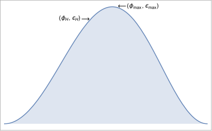
Figure 1: Plot of the slow-roll parameter $\epsilon(\phi)$ showing a maximum for $\phi=\phi_{max}$, close to $\phi_{H}$. The maximum is required because, for observable inflation, $\epsilon(\phi)$ is increasing at $\phi_{H}<\phi_{max}$. At least 8 $e$-folds of inflation should occur in the interval $\phi_{H}<\phi<\phi_{max}$. For $\phi>\phi_{max}$, $\epsilon(\phi)$ can decrease practically generating all of inflation. The maximum of $\epsilon(\phi)$ can not occur at $\phi_{max}=\phi_{H}$ because the value of the tensor-to-scalar ratio $r$ would violate observational bounds. The end of inflation for vanishing $\epsilon(\phi_{e})$ is triggered by a hybrid field and a small $\Delta\phi_{e}$ is obtained when the profile depicted for $\epsilon(\phi)$ is sufficiently thin which, however, should not conflict with the curvature of the potential, controlled by the slow-roll parameter $\eta$.

The derivative of the slow-roll parameter $\epsilon$ at its maximum is

$$\epsilon^{\prime}\equiv\frac{d\epsilon}{d\phi}=\frac{V^{\prime}}{V}\left(\eta-2\epsilon\right)=0,\quad\Longleftrightarrow\quad\eta_{max}=2\epsilon_{max}.$$ (2.4)

As usual, the second derivative of $\epsilon$ at $\eta=2\epsilon$ characterises this critical point

$$\epsilon^{\prime\prime}\Bigl{|}_{\eta=2\epsilon}\equiv\frac{d^{2}\epsilon}{d\phi^{2}}\Bigl{|}_{\eta=2\epsilon}=\left[\xi_{2}-2\eta\epsilon-4\epsilon\left(\eta-2\epsilon\right)+\left(\eta-2\epsilon\right)^{2}\right]\Bigl{|}_{\eta=2\epsilon}=\xi_{2}-4\epsilon^{2},$$ (2.5)

which for a maximum implies that $\xi_{2\,max}<4\epsilon_{max}^{2}$.

Let us concentrate for the moment in the expression where $V^{{}^{\prime}}<0$ with the potential $V$ a monotonically decreasing function of $\phi$ during inflation. In this case $\phi$ is evolving away from the origin, thus the derivative of $\epsilon$ is

$$\epsilon^{\prime}=-\sqrt{2\epsilon}\left(\eta-2\epsilon\right).$$ (2.6)

The case $V^{{}^{\prime}}>0$ would correspond to $\phi$ evolving towards the origin and can be analysed in a similar way. In what follows we parameterise the deviation from the Harrison-Zeldovich spectrum with $\delta_{ns}$ defined by $\delta_{ns}\equiv 1-n_{s}$. We note that Eq. (2.6) together with Eq. (2.2) can be thus written as

$$\epsilon^{\prime}=\frac{1}{2}\sqrt{2\epsilon}\left(\delta_{ns}-2\epsilon\right).$$ (2.7)

Requiring a non-decreasing $\epsilon$ during observable inflation means that there should be at least 8 $e$-folds of inflation between $\phi_{\mathrm{H}}$ and the maximum of $\epsilon$ at $\phi_{max}$. This implies $\epsilon^{\prime}>0$ at least during this range, or

$$\delta_{ns}>2\epsilon>2\epsilon_{H}>0,\$$ (2.8)

which means that during this window of observable inflation the spectral index is bounded by

$$n_{s}<1-2\epsilon_{H}=1-r_{H}/8.$$ (2.9)

In the interval $\phi_{H}<\phi<\phi_{max}$, $\epsilon$ grows from $\epsilon_{H}$ to $\epsilon_{max}$ but its derivative decreases vanishing at $\phi_{max}$ thus $\epsilon_{H}<\epsilon$ and $\epsilon^{\prime}_{H}>\epsilon^{\prime}.$ From Eq. (2.7) we get $1-n_{s}-2\epsilon<\frac{\sqrt{\epsilon_{H}}}{\sqrt{\epsilon}}(1-n_{sH}-2\epsilon_{H})<1-n_{sH}-2\epsilon_{H},$ or

$$n_{s_{H}}<n_{s}+2(\epsilon-\epsilon_{H}),$$ (2.10)

where $\epsilon-\epsilon_{H}>0$. Thus, although $\epsilon$ is larger than $\epsilon_{H}$, $n_{s}$ is not constrained to be smaller than $n_{sH}$ due to the contribution of the $\eta$-term present in $n_{s}$ ($\eta_{H}$-term present in $n_{sH}$).

To find possible consequences for the running let us now consider the second derivative of $\epsilon$. Together with Eq. (2.2), we have

$$\epsilon^{\prime\prime} = \xi_{2}-2\eta\epsilon-4\epsilon\left(\eta-2\epsilon\right)+\left(\eta-2\epsilon\right)^{2}=-9\epsilon^{2}+2\epsilon\delta_{ns}+\frac{1}{4}\delta_{ns}^{2}+\xi_{2}$$ (2.11)

$$= \frac{1}{8}\left(-\frac{9}{32}r^{2}+r\delta_{ns}+2\delta_{ns}^{2}\right)+\xi_{2}.$$

In a similar way, we write the running as

$$n_{sk}=16\epsilon\eta-24\epsilon^{2}-2\xi_{2}=24\epsilon^{2}-8\epsilon\delta_{ns}-2\xi_{2}=\frac{r}{2}\left(\frac{3}{16}r-\delta_{ns}\right)-2\xi_{2}.$$ (2.12)

According to the Planck data (last column of Table 4 of [6]), at $\phi_{H}$, $r_{H}<0.15$, $n_{sH}=0.9644\pm 0.0049$, and $n_{skH}=-0.0085\pm 0.0076$. Thus, $\frac{3}{16}r_{H}-\delta_{nsH}<0$. The running $n_{skH}$ will be negative if and only if

$$\xi_{2H}>\frac{r_{H}}{4}\left(\frac{3}{16}r_{H}-\delta_{nsH}\right)>-5.5\times 10^{-4}.$$ (2.13)

In particular, a positive $\xi_{2H}$ will always give a negative running and from Eq. (2.11), since $-\frac{9}{32}r_{H}^{2}+r_{H}\delta_{nsH}+2\delta_{nsH}^{2}>0$, a positive $\epsilon_{H}^{\prime\prime}$. Furthermore, substituting $\xi_{2}$ from Eq. (2.11) into Eq. (2.12)

$$n_{sk}=-2\epsilon^{\prime\prime}+\frac{1}{128}\left(r-8\delta_{ns}\right)\left(3r-8\delta_{ns}\right).$$ (2.14)

Thus, we conclude that, in general, $n_{sk}$ will be negative if and only if

$$\epsilon^{\prime\prime}>\frac{1}{256}\left(r-8\delta_{ns}\right)\left(3r-8\delta_{ns}\right).$$ (2.15)

The last inequality implies mostly positive values for $\epsilon_{H}^{\prime\prime}$ except in the region where $\delta_{nsH}/6<\epsilon_{H}<\delta_{nsH}/2$, equivalently $8\,\delta_{nsH}/3<r_{H}<8\,\delta_{nsH}$ or $0.082<r_{H}<0.246$, which is still within the bound $r_{H}<0.15$ when running is allowed (see Table 4 of [6]), but interestingly enough, not a zero value either.

When approaching the maximum of $\epsilon$ its derivative $\epsilon^{\prime}$ tends to zero with negative $\epsilon^{\prime\prime}$. A positive value for $\epsilon^{\prime\prime}$ can occur only if in addition $\epsilon(\phi)$ has an inflection point at $\phi_{I}<\phi_{max}$, such that $\epsilon^{\prime}(\phi_{I})$ is a maximum and $\epsilon^{\prime\prime}(\phi_{I})=0$, (see Fig. 2) . In this situation $\phi_{H}$ can be smaller or larger than $\phi_{I}$. Thus, for models where $\epsilon$ presents a maximum with an inflection point as in Fig. 2 , a relatively large $r_{H}$ is most likely accompanied by a negative $\epsilon^{\prime\prime}$ with positive running, while a negligible tensor-to-scalar ratio implies positive $\epsilon^{\prime\prime}$ and negative running. The definitive answer, however, is to be found in the inequality given by Eq. (2.13) which imposes precise constraints on the parameters of an specific model.

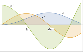
Figure 2: Plot of the slow roll parameter $\epsilon(\phi)$ and its derivatives $\epsilon^{\prime}(\phi)$ and $\epsilon^{\prime\prime}(\phi)$ with respect to $\phi$, as functions of the field, for a model where $\epsilon(\phi)$ is a non-monotonic function of $\phi$. The labels $\phi_{max}$ and $\phi_{I}$ refer to the values of $\phi$ for which the maximum and the inflection points of $\epsilon(\phi)$ occur, respectively.

3 Bounds on $\Delta\phi$ and $r$

While observable scales were leaving the horizon during inflation, $\epsilon$ was an increasing function of $\phi$ and the Lyth bound is regarded as an inevitable consequence. However, if for subsequent $\phi$, we study a decreasing $\epsilon$, then $\epsilon$ has to go through a maximum at $\phi_{max}>\phi_{H}$ before starting to decrease as in Fig. 1.

The value $\phi_{H}$ at which $n_{sH}\approx 0.968$ lies to the left of $\phi_{max}$ so that $\epsilon^{\prime}_{H}$ is positive although small. We observe that an $\epsilon$ with the behaviour shown in Fig. 1 has the potential to generate relatively large values of $r_{H}$ while sufficient inflation is produced away from $\phi_{H}$.

Definig $\Delta\phi_{max}\equiv|\phi_{H}-\phi_{max}|$ and $\Delta N_{max}$ as the corresponding number of $e$-folds generated during the field excursion of width $\Delta\phi_{max}$ the usual expression for the number of $e$-folds gives

$$\Delta N_{max}=\int_{\phi_{H}}^{\phi_{max}}\frac{d\phi}{\sqrt{2\epsilon}}>\Delta\phi_{max}\,\,\mathrm{min}\left\{\frac{1}{\sqrt{2\epsilon}}\right\}=\Delta\phi_{max}\,\,\frac{1}{\sqrt{2\,\mathrm{max}\left\{\epsilon\right\}}}=\frac{\Delta\phi_{max}}{\sqrt{2\epsilon_{max}}},$$ (3.1)

where $\mathrm{min}\left\{...\right\}$ and $\mathrm{max}\left\{...\right\}$ denote the minimum/maximum numerical value of the corresponding quantity in the interval $\Delta\phi_{max}\equiv|\phi_{H}-\phi_{max}|$. However from Eq. (2.7) we have that $2\epsilon_{max}=\delta_{ns,max}$ thus, Eq. (3.1) becomes

$$\Delta\phi_{max}<\Delta N_{max}\sqrt{\delta_{ns,max}}\,.$$ (3.2)

In a similar way

$$\Delta N_{max}=\int_{\phi_{H}}^{\phi_{max}}\frac{d\phi}{\sqrt{2\epsilon}}<\Delta\phi_{max}\,\,\mathrm{max}\left\{\frac{1}{\sqrt{2\epsilon}}\right\}=\Delta\phi_{max}\,\,\left(\frac{1}{\sqrt{2\,\mathrm{min}\{\epsilon\}}}\right)=\frac{\Delta\phi_{max}}{\sqrt{2\epsilon_{H}}}.$$ (3.3)

Consequently, the (slighlty modified) Lyth bound for the interval $\Delta\phi_{max}$ reads

$$\Delta N_{max}\sqrt{\frac{r_{H}}{8}}<\Delta\phi_{max}.$$ (3.4)

Combining Eqs. (3.2) and (3.4) we find a bounded excursion:

$$\Delta N_{max}\sqrt{\frac{r_{H}}{8}}<\Delta\phi_{max}<\Delta N_{max}\sqrt{\delta_{ns,max}}\,.$$ (3.5)

One can also write just the first inequality as a bound for $r_{H}$ which, for the desired upper bound $\Delta\phi_{e}<1$ together with $\Delta\phi_{max}<\Delta\phi_{e}<1$ and $\Delta N_{max}\approx 8$ $e$-folds of observable inflation yields

$$r_{H}\leq 8\left(\frac{\Delta\phi_{max}}{\Delta N_{max}}\right)^{2}<8\left(\frac{\Delta\phi_{e}}{\Delta N_{max}}\right)^{2}<\frac{1}{8}\approx 0.12.$$ (3.6)

This coincides very closely with Planck’s bound. Thus, allowing for an increasing $\epsilon$ during observable inflation with a subsequent decrease, one should be able to construct models where $\Delta\phi_{e}<1$ and with $r_{H}$ saturating the constraints imposed by Planck or Planck-Keck-BICEP2 data.

After the maximum at $\phi_{max}>\phi_{H}$ has been reached, $\epsilon$ starts decreasing up to a point where $1/\sqrt{2\epsilon}$ has generated sufficient $e$-folds and inflation is terminated by a waterfall field. The profile of $\epsilon$ in Fig. 1 implies that close to the end of inflation, at $\phi_{e}$, the potential becomes very flat and a hybrid mechanism should terminate inflation. It is also evident that a small $\Delta\phi_{e}$ is obtained with a sufficiently steep drop in the value of $\epsilon$, thus a feature in $\epsilon$ should not only be high with a low end value but also sharp. We would expect that a sharp feature in $\epsilon$ would conflict with the slow-roll parameter $\eta$ which accounts for the curvature of the potential. In order to control large values of $\eta$ after $\phi$ has reached the maximum, let us rewrite Eq. (2.6) in a more convenient form as

$$\eta=2\epsilon-\frac{\epsilon^{\prime}}{\sqrt{2\epsilon}},\quad\quad\phi>\phi_{max}.$$ (3.7)

After the maximum $\phi_{max}$, $\epsilon^{\prime}$ becomes negative. Consequently, both terms $2\epsilon$ and $-\frac{\epsilon^{\prime}}{\sqrt{2\epsilon}}$ in Eq. (3.7) are positive and thus $0<\eta<1$ during inflation with a decreasing $\epsilon$. The first term is negligible w.r.t. the second because we want a large $\epsilon^{\prime}$, thus for $\phi>\phi_{max}$, $2\epsilon$ decreases while $-\frac{\epsilon^{\prime}}{\sqrt{2\epsilon}}$ grows large

$$\eta=2\epsilon-\frac{\epsilon^{\prime}}{\sqrt{2\epsilon}}\approx-\frac{\epsilon^{\prime}}{\sqrt{2\epsilon}}\approx\frac{\Delta\epsilon_{c}}{\Delta\phi_{c}\sqrt{2\epsilon}}.$$ (3.8)

where $\Delta\epsilon_{c}\equiv|\epsilon_{max}-\epsilon_{e}|$ and $\Delta\phi_{c}\equiv|\phi_{max}-\phi_{e}|$ denote quantities in the complementary range of inflation. Thus, demanding that inflation is sustained for an interval $\Delta\phi_{c}$ (i.e. $\eta<1$), sets a lower bound for

$$\Delta\phi_{c}\approx\frac{\Delta\epsilon_{c}}{\sqrt{2\epsilon}}\,\frac{1}{\eta}>\frac{\Delta\epsilon_{c}}{\sqrt{2\epsilon}}>\frac{\epsilon_{max}-\epsilon_{e}}{\sqrt{2\epsilon_{H}}}\approx\frac{\epsilon_{max}}{\sqrt{2\epsilon_{H}}}\approx\left(\frac{\epsilon_{H}}{2}\right)^{\frac{1}{2}}.$$ (3.9)

In the equation above $\epsilon<\epsilon_{max}$, thus $1/\sqrt{\epsilon}>1/\sqrt{\epsilon_{max}}\approx 1/\sqrt{\epsilon_{H}}$. Using the bound of Eq. (3.6) we get $\Delta\phi_{c}>0.06$, for $\phi>\phi_{max}$ and $\epsilon$ decreasing.

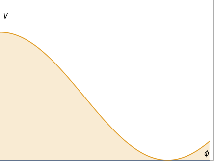
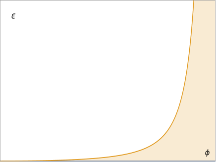
Figure 3: The potential of Natural Inflation with its corresponding tensor-to-scalar ratio (right). Because the minimum of the potential occurs with vanishing energy the (monotonic) tensor-to-scalar ratio diverges at that point. In NI inflation is terminated by the saturation of the condition $\epsilon=1$ with the inflaton also in charge of ending inflation.

4 Examples of models with monotonic and non-monotonic tensors

We illustrate some of the previous discussion with two well motivated models of inflation: Natural Inflation (NI) [17]-[20] and Hybrid Natural Inflation (HNI) [21]-[24].

4.1 A model with a monotonic tensor-to-scalar ratio: Natural Inflation

The NI potential is given by

$$V_{NI}=V_{0}\left[1+\cos\left(\frac{\phi}{f}\right)\right],$$ (4.1)

and from Eq. (2.1) it follows that the tensor-to-scalar ratio $r=16\epsilon$ is given by

$$r=\frac{8}{f^{2}}\frac{\sin^{2}(\frac{\phi}{f})}{\left[1+\cos\left(\frac{\phi}{f}\right)\right]^{2}}.$$ (4.2)

quite clearly r grows without bound diverging for $\phi/f=\pi$, as illustrated in Fig. 3. Typically inflation is terminated when $\epsilon=1.$ In NI not only $\epsilon$ but also $\epsilon^{\prime}$ and $\epsilon^{\prime\prime}$ are monotonically increasing functions of $\phi$.

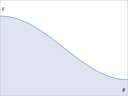
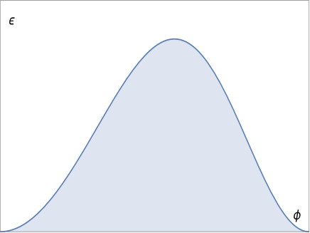
Figure 4: In Hybrid Natural Inflation there is a nearly flat plateau followed by a smooth fast transition to a lower flat constant plateau where most of inflation can occur and where inflation is terminated by a second waterfall-field. After the inflaton $\phi$ has carried out all of inflation the waterfall-field fast-roll towards the global minimum with vanishing energy (not shown). As a consequence of this the inflaton minimum has a non-vanishing energy (left) allowing for the possibility of a non-monotonic tensor-to-scalar ratio (right).

4.2 A model with a non-monotonic tensor-to-scalar ratio: Hybrid Natural Inflation

In HNI [21]-[24] all of inflation is driven by the single-field $\phi$ although the end of inflation is triggered by a second, waterfall-field. The inflationary sector of HNI is

$$V_{HNI}=V_{0}\left[1+a\cos\left(\frac{\phi}{f}\right)\right],$$ (4.3)

where $0\leq a<1$. The tensor-to-scalar ratio is given by

$$r=\frac{8}{f^{2}}\frac{a^{2}\sin^{2}(\frac{\phi}{f})}{\left[1+a\cos\left(\frac{\phi}{f}\right)\right]^{2}}.$$ (4.4)

We see that $r=0$ at $\phi/f=0,\pi$ developing a maximum located at $\cos(\phi_{max}/f)=-a$ (see Fig. 4). The maximum value $r$ can take (away from $r_{H}$) is therefore $r_{max}=\frac{8a^{2}}{f^{2}(1-a^{2})}$. In both cases the running can be written as [24]

$$n_{sk}=\frac{r}{32}\left(3r-16\delta_{ns}+\frac{8}{f^{2}}\right),$$ (4.5)

without $a$ appearing explicitly. Thus, the running $n_{skH}$ will be negative if and only if

$$f>\frac{1}{\sqrt{2\delta_{ns}-\frac{3}{8}r}}.$$ (4.6)

According to the values of Table 4 of Planck data [6] we get $f>3.5$, in Planck units. In NI $f$ is strictly super-Planckian satisfying the previous bound with a negative running while in HNI $f$ can also be sub-Planckian with positive running allowing for the possibility of primordial black hole production during inflation [14], [24].

5 Conclusions

We developed a model-independent study of single field slow-roll canonical inflation by imposing conditions on the slow-roll parameter $\epsilon(\phi)$ and its derivatives, $\epsilon^{\prime}(\phi)$ and $\epsilon^{\prime\prime}(\phi)$, to extract general conditions on the tensor-to-scalar ratio $r$ and the running $n_{sk}$. For models where $\epsilon(\phi)$ presents a maximum, a relatively large $r_{H}$ is most likely accompanied by a positive running, while a negligible tensor-to-scalar ratio typically implies negative running. The definitive answer, however, is given by the condition on the slow-roll parameter $\xi_{2}$, Eq. (2.13). We have also shown that by imposing conditions to the slow-roll parameter $\epsilon(\phi)$ and its derivatives $\epsilon^{\prime}(\phi)$ and $\epsilon^{\prime\prime}(\phi)$ we can accommodate sufficient inflation with a relatively large $r_{H}$ but still satisfying the Planck [6] or Planck-Keck-BICEP2 [7] constraints. The excursion of the field $\Delta\phi_{e}\equiv|\phi_{H}-\phi_{e}|$ will be no larger than one if the function $\epsilon(\phi)$ has a maximum in a thin hill-shaped feature, decreasing to small values close to the end of inflation, at $\phi_{e}$. The maximum is required because observations indicate that $\epsilon_{H}$ is increasing in the observables scales, at $\phi_{H}$. Then $\epsilon(\phi)$ should decrease for $\phi>\phi_{max}$ for an effective way of generating the majority of $e$-folds of inflation. The contribution to the number of $e$-folds when $\epsilon{(\phi)}$ is growing can be 8 $e$-folds for $\Delta\phi_{e}$ less than one and $r_{H}$ close to the upper limit $r_{H}=0.12$. The end of inflation for vanishing $\epsilon(\phi)$ can be triggered by a hybrid field and a small $\Delta\phi_{c}\equiv|\phi_{max}-\phi_{e}|$ is obtained when $\epsilon(\phi)$ is sufficiently thin which, however, should not conflict with the other slow-roll parameter $\eta(\phi)$. Under these circumstances $\Delta\phi_{e}$ is restricted to a narrow windows of values.

6 Acknowledgements

G.G. gratefully acknowledges hospitality of the Rudolf Peierls Centre for Theoretical Physics, Oxford and useful discussions with Prof. Graham G. Ross and Shaun Hotchkiss. He also acknowledges financial support from PASPA-DGAPA, UNAM and CONACYT, Mexico. We all acknowledge support from Programa de Apoyo a Proyectos de Investigación e Innovación Tecnológica (PAPIIT) UNAM, IN103413-3, Teorías de Kaluza-Klein, inflación y perturbaciones gravitacionales, IA101414, Fluctuaciones No-Lineales en Cosmología Relativista and IA103616, Observables en Cosmología Relativista. AHA is also grateful to SNI and PRODEP for partial financial support, and acknowledges a VIEP-BUAP-HEAA-EXC15-I research grant.

References

- [1] A.H. Guth, The Inflationary Universe: A possible solution to the horizon and flatness problems Phys. Rev. D23 (1981) 347.
- [2] A.D Linde, A New Inflationary Universe Scenario: A Possible Solution of the Horizon, Flatness, Homogeneity, Isotropy and Primordial Monopole Problems Phys. Lett. B108 (1982) 389.
- [3] A. Albrecht and P.J. Steinhardt, Cosmology for Grand Unified Theories with Radiatively Induced Symmetry Breaking Phys. Rev. Lett. 48 (1982) 1220.
- [4] For reviews see e.g., D. H. Lyth and A. Riotto, Particle physics models of inflation and the cosmological density perturbation, Phys. Rept. 314 (1999) 1 [hep-ph/9807278]; D. H. Lyth and A. R. Liddle, The primordial density perturbation: Cosmology, inflation and the origin of structure, Cambridge, UK: Cambridge Univ. Pr. (2009) 497 p; D. Baumann, TASI Lectures on Inflation, arXiv:0907.5424 [hep-th].
- [5] W. Hu, Generalized Slow Roll for Non-Canonical Kinetic Terms, Phys. Rev. D 84 (2011) 027303 [arXiv:1104.4500 [astro-ph.CO]].
- [6] P. A. R. Ade et al. [Planck Collaboration], Planck 2015 results. XX. Constraints on inflation, arXiv:1502.02114 [astro-ph.CO].
- [7] P. A. R. Ade et al. [BICEP2 and Planck Collaborations], Joint Analysis of BICEP2/Keck Array and Planck Data, Phys. Rev. Lett. 114 (2015) 101301 [arXiv:1502.00612 [astro-ph.CO]].
- [8] D. H. Lyth, What would we learn by detecting a gravitational wave signal in the cosmic microwave background anisotropy? Phys. Rev. Lett. 78(1997)1861 [hep-ph/0502047].
- [9] L. Boubekeur and D. H. Lyth, Hilltop inflation, JCAP 0507 (2005) 010 [hep-ph/0502047].
- [10] I. Ben-Dayan and R. Brustein, “Cosmic Microwave Background Observables of Small Field Models of Inflation,” JCAP 1009 (2010) 007 [arXiv:0907.2384 [astro-ph.CO]].
- [11] S. Hotchkiss, A. Mazumdar and S. Nadathur, “Observable gravitational waves from inflation with small field excursions,” JCAP 1202 (2012) 008 [arXiv:1110.5389 [astro-ph.CO]].
- [12] S. Antusch and D. Nolde, BICEP2 implications for single-field slow-roll inflation revisited, arXiv:1404.1821 [hep-ph].
- [13] A. Chatterjee and A. Mazumdar, Bound on largest from sub-Planckian excursions of inflaton, JCAP 1501 (2015) 01, 031 doi:10.1088/1475-7516/2015/01/031 [arXiv:1409.4442 [astro-ph.CO]].
- [14] K. Kohri, D. H. Lyth and A. Melchiorri, Black hole formation and slow-roll inflation, JCAP 0804 (2008) 038 [arXiv:0711.5006 [hep-ph]].
- [15] J. A. Vazquez, M. Carrillo-Gonzalez, G. German, A. Herrera-Aguilar and J. C. Hidalgo, “Constraining Hybrid Natural Inflation with recent CMB data,” JCAP 1502 (2015) 02, 039 [arXiv:1411.6616 [astro-ph.CO]].
- [16] A. R. Liddle and D. H. Lyth, Cosmological Inflation and Large-Scale Structure, Cambridge University Press, (2000).
- [17] K. Freese, J. A. Frieman and A. V. Olinto, Natural inflation with pseudo - Nambu-Goldstone bosons, Phys. Rev. Lett. 65 (1990) 3233.
- [18] F. Adams, J.R. Bond, K. Freese, J. A. Frieman and A. V. Olinto, Natural inflation: Particle physics models, power law spectra for large scale structure, and constraints from COBE Phys. Rev.D47 (1993) 426-455.
- [19] K. Freese, C. Savage and W. H. Kinney, Natural Inflation: the status after WMAP 3-year data, Int. J. Mod. Phys. D 16 (2008) 2573 [arXiv:0802.0227 [hep-ph]].
- [20] K. Freese and W. H. Kinney, Natural Inflation: Consistency with Cosmic Microwave Background Observations of Planck and BICEP2, arXiv:1403.5277 [astro-ph.CO].
- [21] G. G. Ross and G. German, Hybrid natural inflation from non Abelian discrete symmetry, Phys. Lett. B 684 (2010) 199 [arXiv:0902.4676 [hep-ph]].
- [22] G. G. Ross and G. German, Hybrid Natural Low Scale Inflation, Phys. Lett. B 691 (2010) 117 [arXiv:1002.0029 [hep-ph]].
- [23] M. Carrillo-Gonzalez, G. German, A. Herrera-Aguilar, J. C. Hidalgo and R. Sussman, Testing Hybrid Natural Inflation with BICEP2, Phys. Lett. B 734 (2014) 345 [arXiv:1404.1122 [astro-ph.CO]].
- [24] G. G. Ross, G. German and J. A. Vazquez, Hybrid Natural Inflation, arXiv:1601.03221 [astro-ph.CO].