Dynamical Instability of Gaseous Sphere in the Reissner-Nordström Limit

Abstract

In this paper, we study the dynamical instability of gaseous sphere under radial oscillations approaching the Reissner-Nordström limit. For this purpose, we derive linearized perturbed equation of motion following the Eulerian and Lagrangian approaches. We formulate perturbed pressure in terms of adiabatic index by employing the conservation of baryon numbers. A variational principle is established to evaluate characteristic frequencies of oscillations which lead to the criteria for dynamical stability. The dynamical instability of homogeneous sphere as well as relativistic polytropes with different values of charge in Newtonian and post-Newtonian regimes is explored. We also find their radii of instability in terms of the Reissner-Nordstörm radius. We conclude that dynamical instability occurs if the gaseous sphere contracts to the Reissner-Nordstörm radius for different values of charge.

Keywords: Gravitational collapse; Instability; Electromagnetic field; Relativistic fluids.
PACS: 04.20.-q; 04.25.Nx; 04.40.Dg; 04.40.Nr.

1 Introduction

It is a well-known fact that any relativistic model will be physically interesting if it is stable under fluctuations. The stability/instability of celestial objects has significant importance in general relativity (GR). This study is closely related to the evolution and structure formation of self-gravitating objects. Initially, any stable gaseous mass remains in state of hydrostatic equilibrium for which the gravitational force is counter balanced by the internal pressure of the body acting in the opposite direction. The effect of gravity over the internal pressure causes the matter to collapse and the star contracts to a point under its own gravitational force forming compact stars.

The dynamics of massive stars can be discussed in weak as well as strong-field regimes. The idea of weak-field approximation (Newtonian and post-Newtonian approximations (pN)) [1] has remarkable importance in the context of relativistic hydrodynamics. The analysis of dynamical instability in strong-field regimes becomes complicated due to non-linear terms, so the weak-field approximation schemes are used as an effective tool. Chandrasekhar [2] was the pioneer who studied the dynamical instability of Newtonian perfect fluid sphere approaching the Schwarzschild limit in terms of adiabatic index. He used Eulerian approach for hydrodynamic equations and developed a variational principle to find characteristic frequencies applicable to the radial oscillations at Newtonian and pN limits. He concluded that the system would be dynamically stable or unstable according to the numerical value of adiabatic index, i.e., $\Gamma>\frac{4}{3}$ or $\Gamma<\frac{4}{3}$, respectively. The same author [3] also investigated the stability of gaseous sphere under radial and non-radial oscillations at pN limit.

The dynamical instability of self-gravitating spherical objects has been studied by using various techniques. Herrera et al. [4] explored dynamical instability of spherical collapsing system for non-adiabatic fluid using perturbation scheme. They showed that heat conduction increases the instability range in Newtonian limit but decreases in pN limit. Later, many researchers [5] discussed the role of various physical factors on the dynamical instability of spherical systems using perturbation scheme and found interesting results.

The stability of self-gravitating objects in the presence of electromagnetic field has a primordial history starting with Rosseland [6]. There is a general consensus that astrophysical objects do not have charge in large amount [7] but there are some mechanisms which induce large amount of electric charge in collapsing stars. Stettner [8] showed that presence of net surface charge enhances the stability of sphere with uniform density. Glazer [9] investigated the dynamical stability of perfect fluid sphere pulsating radially with electric charge. Ghezzi [10] studied stability of neutron stars and found that the stars having a charge greater than the extreme value would explode. Sharif and collaborators [11] discussed the role of electric charge in dynamical instability at Newtonian and pN regimes.

Polytropes are useful self-gravitating objects as they provide simplified models for internal structures of stellar objects. The polytropic equation of state deals with various fundamental astrophysical issues [12]. Tooper [13] studied the internal structure of gaseous sphere obeying polytropic equation of state and obtained Newtonian polytropes using numerical solution of the Lane-Emden equation. The effect of electromagnetic field on the dynamics of polytropic compact stars has also been studied [14]. Herrera and Barreto [15] analyzed both Newtonian as well as relativistic polytropes in spherical symmetry. Recently, Breysse et al. [16] have discussed the dynamical instability of cylindrical polytropic fluid systems under radial and non-radial modes of oscillations.

In this paper, we study the dynamical instability of spherically symmetric gaseous systems following Chandrasekhar’s approach [2] in the vicinity of electromagnetic field. The paper is organized as follows. The next section deals with matter distribution and the Einstein-Maxwell field equations. In section 3, we discuss motion of the system under radial oscillations following the Eulerian approach. Section 4 provides the formulation of perturbed pressure and adiabatic index in terms of Lagrangian displacement using conservation of baryon number. In section 5, we develop conditions for dynamical instability of homogeneous sphere and relativistic polytropes. Finally, we conclude our results in the last section.

2 Field Equations and Matter Configuration

We consider a spherically symmetric system in the interior region given by

$$ds^{2}=-e^{\nu}dt^{2}+e^{\lambda}dr^{2}+r^{2}(d\theta^{2}+\sin^{2}\theta d\phi^{2}),$$ (1)

where $\nu=\nu(t,r)$ and $\lambda=\lambda(t,r)$ are the gravitational potentials. The corresponding Einstein field equations can be written as

$$-\frac{8\pi G}{c^{4}}T_{0}^{0} = \frac{1}{r^{2}}-\frac{1}{r^{2}}\frac{\partial}{\partial r}(re^{-\lambda}),$$ (2)

$$-\frac{8\pi G}{c^{4}}T_{1}^{1} = \frac{1}{r^{2}}-e^{-\lambda}(\frac{1}{r^{2}}+\frac{1}{r}\frac{\partial\nu}{\partial r}),$$ (3)

$$\frac{8\pi G}{c^{4}}T_{0}^{1} = \dot{\lambda}\frac{e^{-\lambda}}{r},$$ (4)

where dot denotes derivative w.r.t $t$. We assume the energy-momentum tensor corresponding to charged perfect fluid in the form

$$T_{j}^{i}=(\sigma+p)u^{i}u_{j}+p\delta_{j}^{i}+\frac{1}{4\pi}[F_{jk}F^{ik}-\frac{1}{4}\delta_{j}^{i}F_{kl}F^{kl}],$$ (5)

where $u^{i}=\frac{dx^{i}}{ds}$ is the four-velocity, $p$ is the pressure and $\sigma$ is the energy density. The electromagnetic field tensor $F_{ij}$ can be defined in terms of four potential, $F_{ij}=\Phi_{j;i}-\Phi_{i;j}$, which satisfies the Maxwell field equations as

$$F^{ij}_{~{};j}=4\pi J^{i},\quad F_{[ij,k]}=0,$$

where $J^{i}=\rho u^{i}$ is the four current. The only non-vanishing radial component of electromagnetic field tensor ($F^{01}=-F^{10}$) implies that

$$\frac{d\left(r^{2}e^{(\lambda+\nu)/2}F^{01}\right)}{dr}=4\pi r^{2}e^{\lambda/2}\rho,$$

whose integration yields

$$F^{01}=\frac{e^{-(\lambda+\nu)/2}Q(t,r)}{r^{2}},$$

where $Q(t,r)=4\pi\int_{0}^{r}r^{2}\rho e^{\lambda/2}dr$ is the total amount of charge within the sphere.

The energy-momentum tensor follows the conservation identity $T_{~{};j}^{ij}=0$, which governs hydrodynamics of the fluid and leads to the following relations

$$\frac{\partial T_{0}^{0}}{\partial t}+\frac{\partial T_{1}^{0}}{\partial r}+\frac{1}{2}\left(\frac{4}{r}+\frac{\partial}{\partial r}(\lambda+\nu)\right)T_{0}^{1}+\frac{1}{2}\left(T_{0}^{0}-T_{1}^{1}\right)\frac{\partial\lambda}{\partial t}=0,$$ (6)

$$\frac{\partial T_{1}^{0}}{\partial t}+\frac{\partial T_{1}^{1}}{\partial r}+\frac{1}{2}\left(T_{1}^{1}-T_{0}^{0}\right)\frac{\partial\nu}{\partial r}-\frac{2}{r}\left(p-T_{1}^{1}\right)+\frac{1}{2}T_{1}^{0}\frac{\partial}{\partial t}(\lambda+\nu)=0,$$ (7)

where $T_{0}^{1}=-e^{\nu-\lambda}T_{1}^{0}$. The non-zero components of energy-momentum tensor are

$$T^{0}_{0}=-\sigma-\frac{Q^{2}}{8\pi r^{4}},\quad T^{1}_{1}=p-\frac{Q^{2}}{8\pi r^{4}},\quad T^{2}_{2}=T^{3}_{3}=p+\frac{Q^{2}}{8\pi r^{4}}.$$

All the quantities governing the motion remain independent of time during the state of hydrostatic equilibrium. The surface stresses describing equilibrium state are denoted by zero subscript. In this context, Eqs.(2), (3) and (7) take the form

$$\frac{d}{dr}(re^{-\lambda_{0}}) = 1-\frac{8\pi Gr^{2}}{c^{4}}\sigma_{0}-\frac{GQ^{2}}{c^{4}r^{2}},$$ (8)

$$\frac{1}{r}e^{-\lambda_{0}}\frac{d\nu_{0}}{dr} = \frac{1}{r^{2}}(1-e^{-\lambda_{0}})+\frac{8\pi Gp_{0}}{c^{4}}-\frac{GQ^{2}}{c^{4}r^{4}},$$ (9)

$$\frac{dp_{0}}{dr} = \frac{1}{2}\frac{d\nu_{0}}{dr}(p_{0}+\sigma_{0})+\frac{1}{8\pi}\frac{d}{dr}\left(\frac{Q^{2}}{r^{4}}\right)+\frac{Q^{2}}{4\pi r^{5}}.$$ (10)

Following Eqs.(2) and (3), we also have a useful relation

$$\frac{e^{-\lambda_{0}}}{r}\frac{d}{dr}(\lambda_{0}+\nu_{0})=(p_{0}+\sigma_{0})\frac{8\pi G}{c^{4}}.$$ (11)

We take the Reissner-Nordström (RN) spacetime in the exterior region as

$$ds^{2} = -\left(1-\frac{2GM}{rc^{2}}+\frac{GQ^{2}}{r^{2}c^{4}}\right)dt^{2}+\left(1-\frac{2GM}{rc^{2}}+\frac{GQ^{2}}{r^{2}c^{4}}\right)^{-1}dr^{2}$$ (12)

$$+ r^{2}(d\theta^{2}+\sin^{2}\theta d\phi^{2}),$$

where $M$ corresponds to the total mass of the sphere. The hydrostatic equilibrium describes the state of fluid in which pressure gradient force is balanced by the gravitational force. When one of these forces overcome the other, the stability of the system is disturbed leading to an unstable system. The equation describing hydrostatic equilibrium is obtained by eliminating $\nu_{0}$ from Eqs.(9) and (10) as

$$\left(1-\frac{2GM_{r}}{rc^{2}}+\frac{GQ^{2}}{r^{2}c^{4}}\right)\frac{dp_{0}}{dr}=-\frac{1}{c^{2}}\left(\frac{GM_{r}}{r^{2}}-\frac{GQ^{2}}{r^{3}c^{2}}+\frac{4\pi G}{c^{2}}pr\right)$$

$$\times(p_{0}+\sigma_{0})+\frac{1}{4\pi}\left(1-\frac{2GM_{r}}{rc^{2}}+\frac{GQ^{2}}{r^{2}c^{4}}\right)\left(\frac{Q^{2}}{r^{5}}+\frac{1}{2}\frac{d}{dr}\left(\frac{Q^{2}}{r^{5}}\right)\right),$$ (13)

where the left and right hand sides correspond to pressure gradient and gravitational terms, respectively and

$$M_{r}=\frac{4\pi G}{c^{4}}\int_{0}^{r}\sigma_{0}r^{2}dr+\frac{G}{2c^{4}}\int_{0}^{r}\frac{Q^{2}}{r^{2}}dr,$$ (14)

is the Misner-Sharp mass function.

3 Equations Governing Radial Oscillations

Here we discuss the motion of gaseous masses undergoing radial oscillations. The non-zero components of four-velocity are given by

$$u^{0}=e^{-\frac{\nu_{0}}{2}},\quad u_{0}=-e^{\frac{\nu_{0}}{2}},\quad u^{1}=ve^{-\frac{\nu_{0}}{2}},\quad u_{1}=ve^{\frac{\lambda_{0}-\nu_{0}}{2}},$$ (15)

where $v=\frac{dr}{dt}$ is the radial velocity component. These components can be calculated with respect to spacetime coordinates by $u^{i}=\frac{dx^{i}}{ds}$. The stability of any gaseous mass under perturbation ultimately gives rise to the dynamical evolution of gravitating system. We assume that an equilibrium configuration is perturbed such that it does not affect the spherical symmetry. We consider only linear terms so that the respective values in the perturbed state become

$$\lambda=\lambda_{0}+\delta\lambda,\quad\nu=\nu_{0}+\delta\nu,\quad p=p_{0}+\delta p,\quad\sigma=\sigma_{0}+\delta\sigma,\quad Q=Q_{0}+\delta Q.$$ (16)

We follow the Eulerian approach [3] for perturbations such that the corresponding linearized forms (governing the radial perturbations) through Eqs.(8) and (9) are

$$\frac{\partial}{\partial r}(re^{-\lambda_{0}}\delta\lambda)=\frac{2G}{c^{4}}\left(4\pi r^{2}\delta\sigma-\frac{Q_{0}\delta Q}{r^{2}}\right),$$ (17)

$$\frac{e^{-\lambda_{0}}}{r}\left[\frac{\partial}{\partial r}\delta\nu-\delta\lambda\frac{d\nu_{0}}{dr}\right]=\frac{1}{r^{2}}e^{-\lambda_{0}}\delta\lambda+\frac{8\pi G}{c^{4}}\delta p-\frac{2GQ_{0}\delta Q}{c^{4}r^{4}},$$ (18)

here $\delta\lambda$, $\delta\nu$, $\delta\sigma$, $\delta p$ and $\delta Q$ represent the Eulerian changes. Equations (4) and (7) can be written appropriately in linearized forms as

$$\frac{e^{-\lambda_{0}}}{r}\frac{\partial}{\partial t}\delta\lambda=-\frac{4\pi G}{c^{4}}\left(2(p_{0}+\sigma_{0})v-\frac{Q_{0}\delta Q}{r^{4}}\right),$$ (19)

$$(p_{0}+\sigma_{0})e^{\lambda_{0}-\nu_{0}}\frac{\partial v}{\partial t}+\frac{\partial}{\partial r}\delta p+\frac{1}{2}(p_{0}+\sigma_{0})\frac{\partial}{\partial r}\delta\nu$$

$$+\frac{1}{2}(\delta p+\delta\sigma)\frac{d\nu_{0}}{dr}+\frac{1}{8\pi}\frac{Q_{0}\delta Q}{r^{4}}-\frac{1}{4\pi}\frac{\partial}{\partial r}\left[\frac{Q_{0}\delta Q}{r^{4}}\right]=0.$$ (20)

Let us introduce a Lagrangian displacement $``\eta"$ such that $v=\frac{\partial\eta}{\partial t}$. Integration of Eq.(19) leads to

$$\frac{e^{-\lambda_{0}}}{r}\delta\lambda=-\frac{8\pi G}{c^{4}}(p_{0}+\sigma_{0})\eta+\frac{4\pi GQ_{0}}{c^{4}r^{4}}\int\delta Qdt.$$ (21)

Using Eq.(11), this equation takes the form

$$\delta\lambda=-\frac{d}{dr}(\lambda_{0}+\nu_{0})\eta+\frac{4\pi GQ_{0}e^{\lambda_{0}}}{c^{4}r^{3}}\int\delta Qdt.$$ (22)

Solving Eq.(17) and (21), it follows that

$$\delta\sigma=\frac{1}{r^{2}}\frac{\partial}{\partial r}\left[-r^{2}(\sigma_{0}+p_{0})\eta+\frac{Q^{2}}{2r^{4}}\int\delta Qdt\right]+\frac{Q_{0}}{4\pi r^{4}}\delta Q,$$ (23)

which yields

$$\delta\sigma = -\eta\frac{dp_{0}}{dr}-\eta\frac{d\sigma_{0}}{dr}-\frac{1}{r^{2}}(p_{0}+\sigma_{0})\frac{\partial}{\partial r}(\eta r^{2})+\frac{1}{r^{2}}\frac{\partial}{\partial r}\left[\frac{Q_{0}}{2r^{4}}\int\delta Qdt\right]$$ (24)

$$+ \frac{Q_{0}}{4\pi r^{4}}\delta Q.$$

Using Eq.(10), it follows that

$$\delta\sigma = -\eta\frac{d\sigma_{0}}{dr}-\frac{e^{\nu_{0}/2}}{r^{2}}(p_{0}+\sigma_{0})\frac{\partial}{\partial r}\left[\eta r^{2}e^{-{\nu_{0}/2}}\right]-\frac{\eta}{8\pi}\frac{d}{dr}\left[\frac{Q^{2}}{r^{4}}\right]$$ (25)

$$+ \frac{1}{r^{2}}\frac{\partial}{\partial r}\left[\frac{Q_{0}}{2r^{4}}\int\delta Qdt\right]+\frac{Q_{0}}{4\pi r^{4}}\delta Q.$$

Substituting $\delta\lambda$ from Eq.(21) in (18), we obtain

$$\frac{e^{-\lambda_{0}}}{r}\frac{\partial}{\partial r}\delta\nu = \left[(p_{0}+\sigma_{0})\left(\frac{1}{r}+\frac{d\nu_{0}}{dr}\right)\eta+\delta p\right]\frac{8\pi G}{c^{4}}$$ (26)

$$+ \frac{4\pi GQ_{0}}{c^{4}r^{4}}\left[\frac{d\nu_{0}}{dr}-\frac{\eta}{r}\right]\int\delta Qdt-\frac{2GQ_{0}}{c^{4}r^{4}}\delta Q,$$

which in accordance of Eq.(11) leads to

$$(p_{0}+\sigma_{0})\frac{\partial}{\partial r}\delta\nu = \frac{d}{dr}(\lambda_{0}+\nu_{0})\left\{\left[\delta p-(p_{0}+\sigma_{0})\left(\frac{1}{r}+\frac{d\nu_{0}}{dr}\right)\eta\right]\right.$$ (27)

$$+ \left.\frac{Q_{0}}{2r^{4}}\left[\frac{d\nu_{0}}{dr}-\frac{\eta}{r}\right]\int\delta Qdt-\frac{Q_{0}}{4\pi r^{4}}\delta Q\right\}.$$

Now we assume time dependent perturbations in the form of Lagrangian displacement, i.e., $\eta e^{i\omega t}$, where $\omega$ is the characteristic frequency to be evaluated. The Lagrangian displacement $\eta$ connects the fluids elements in equilibrium with corresponding one in the perturbed configuration. Since the equations have natural modes of oscillations, so they will depend on time. Considering $\delta\lambda,~{}\delta\nu,$ $\delta p,~{}\delta\sigma$ and $\delta Q$ as time dependent amplitudes of the respective quantities, Eq.(20) with (27) can be rewritten as

$$\omega^{2}e^{\lambda_{0}-\nu_{0}}(p_{0}+\sigma_{0})\eta = \delta p\frac{d}{dr}\left(\nu_{0}+\frac{1}{2}\lambda_{0}\right)+\frac{d}{dr}\delta p+\frac{1}{2}\delta\sigma\frac{d\nu_{0}}{dr}-\frac{1}{2}(p_{0}+\sigma_{0})$$ (28)

$$\times \left(\frac{d\nu_{0}}{dr}+\frac{d\lambda_{0}}{dr}\right)\left(\frac{1}{r}+\frac{d\nu_{0}}{dr}\right)\eta+\frac{Q_{0}}{8\pi r^{4}}\frac{d}{dr}(\lambda_{0}+\nu_{0})$$

$$\times \left\{2\pi\left(\frac{d\nu_{0}}{dr}-\frac{\eta}{r}\right)\int\delta Qdt-\delta Q\right\}+\frac{1}{4\pi}\left\{\frac{Q_{0}\delta Q}{2r^{4}}\right.$$

$$- \left.\frac{d}{dr}\left(\frac{Q_{0}\delta Q}{r^{4}}\right)\right\}.$$

4 The Conservation of Baryon Number

In order to discuss the perturbed state of pressure in terms of Lagrangian displacement $\eta$, an additional assumption is required which can relate physical aspects of relativistic theory with the gaseous mass undergoing adiabatic radial oscillations. In this context, the required supplementary condition can be satisfied by conservation of baryon number in the framework of GR as $(Nu^{j})_{;j}=0$, or

$$\frac{\partial}{\partial x^{j}}(Nu^{j})+Nu^{j}\frac{\partial}{\partial x^{j}}\ln\sqrt{-g}=0,$$ (29)

where $N$ is the baryon number per unit volume. The conservation of baryon number plays a vital role in collecting different models of the universe. According to this law, the number of particles may vary but their total number will remain conserved during the fluid flow. This change occurs due to loss or gain of net fluxes. Here we consider fluid obeying this identity. Equation (29) through (15) leads to

$$\frac{\partial}{\partial t}(Ne^{-\nu_{0}/2})+\frac{\partial}{\partial r}(Nve^{-\nu_{0}/2})+Nve^{-\nu_{0}/2}\frac{\partial}{\partial r}\left(\frac{2}{r}+\frac{1}{2}[\nu+\lambda]\right)$$

$$+\frac{N}{2}e^{-\nu_{0}/2}\frac{\partial}{\partial t}(\nu+\lambda)=0.$$ (30)

We assume the perturbation

$$N=N_{0}(r)+\delta N(r,t),$$ (31)

keeping only the linear terms in $v$, Eq.(30) takes the form

$$\frac{1}{r^{2}}\frac{\partial}{\partial r}(N_{0}r^{2}ve^{-\nu_{0}/2})+e^{-\nu_{0}/2}\frac{\partial}{\partial t}\delta N+\frac{1}{2}N_{0}e^{-\nu_{0}/2}\frac{d}{dr}(\nu_{0}+\lambda_{0})$$

$$+\frac{1}{2}N_{0}e^{-\nu_{0}/2}\frac{\partial}{\partial t}\delta\lambda=0,$$ (32)

whose integration in terms of Lagrangian displacement $\eta$ leads to

$$\delta N+\frac{N_{0}}{2}\left[\eta\frac{d}{dr}(\nu_{0}+\lambda_{0})+\delta\lambda\right]+\frac{1}{r^{2}}e^{\nu_{0}/2}\frac{\partial}{\partial r}\left(N_{0}r^{2}\eta e^{-\nu_{0}/2}\right)=0.$$ (33)

Using Eq.(22), it follows that

$$\delta N=-\eta\frac{dN_{0}}{dr}-\frac{N_{0}}{r^{2}}e^{\nu_{0}/2}\frac{\partial}{\partial r}\left(r^{2}\eta e^{-\nu_{0}/2}\right)+\frac{2\pi GN_{0}Q_{0}}{c^{4}r^{3}}e^{\lambda_{0}}\int\delta Qdt.$$ (34)

We consider an equation of state in the form

$$N=N(\sigma,p),$$ (35)

so that Eqs.(25) and (34) together give

$$\delta p=-\eta\frac{dp_{0}}{dr}-p_{0}\Gamma\frac{e^{\nu_{0}/2}}{r^{2}}\frac{\partial}{\partial r}\left(r^{2}\eta e^{-\nu_{0}/2}\right)+\frac{\alpha Q_{0}}{r^{3}}\int\delta Qdt,$$ (36)

where

$$\alpha=\frac{1}{\partial N/\partial p}\left\{\frac{2\pi GN_{0}}{c^{4}}e^{\lambda_{0}}-\frac{1}{2r}\frac{dN}{d\sigma}\right\},$$ (37)

and $\Gamma$ is the adiabatic index (ratio of specific heats) defined by

$$\Gamma=\frac{1}{p\partial N/\partial p}\left\{N-(\sigma+p)\frac{\partial N}{\partial\sigma}\right\}.$$ (38)

This relates the pressure and density fluctuations and measures the stiffness of the fluid.

5 Pulsation Equation and Variational Principle

The linear pulsation corresponds to the oscillation frequencies and different modes of small perturbations applied to equilibrium spherical configuration. Inserting the values of $\delta\sigma$ and $\delta p$ from Eqs.(23) and (36) in (28), it follows that

$$\omega^{2}e^{\lambda_{0}-\nu_{0}}(p_{0}+\sigma_{0})\eta=-\eta\left(\frac{d\nu_{0}}{dr}+\frac{1}{2}\frac{d\lambda_{0}}{dr}\right)\frac{dp_{0}}{dr}-\frac{d}{dr}\left(\eta\frac{dp_{0}}{dr}\right)-\frac{1}{2}\left\{\frac{2}{r}\right.$$

$$\times\left.(p_{0}+\sigma_{0})\eta+\frac{d}{dr}[(p_{0}+\sigma_{0})\eta]\right\}-\frac{1}{2}\eta(p_{0}+\sigma_{0})\left(\frac{d\nu_{0}}{dr}+\frac{d\lambda_{0}}{dr}\right)\left(\frac{1}{r}+\frac{d\nu_{0}}{dr}\right)$$

$$-e^{-(\nu_{0}+\frac{\lambda_{0}}{2})}\frac{d}{dr}\left\{e^{(\nu_{0}+\frac{\lambda_{0}}{2})}\Gamma p_{0}\frac{e^{\nu_{0}/2}}{r^{2}}\frac{d}{dr}(r^{2}\eta e^{-\nu_{0}/2})\right\}+e^{-\lambda_{0}/2}\frac{d}{dr}\left\{\frac{\beta Q_{0}}{r^{3}}\right.$$

$$\times\left.e^{\lambda_{0}/2}\int\delta Qdt\right\}+\frac{Q_{0}}{r^{3}}\frac{d\nu_{0}}{dr}\int\delta Qdt\left\{\beta+\frac{1}{4r}+\frac{1}{4\pi r}\left(\frac{d\nu_{0}}{dr}-\frac{\eta}{r}\right)\right\}$$

$$+\frac{Q_{0}}{4\pi r^{4}}\frac{d\lambda_{0}}{dr}\left\{\frac{d\nu_{0}}{dr}-\frac{\eta}{r}\int\delta Qdt-\frac{\delta Q}{2}\right\}+\frac{Q_{0}}{8\pi r^{4}}\delta Q+\frac{e^{\nu_{0}/2}}{4\pi}\frac{d}{dr}\left\{\frac{Q_{0}e^{\nu_{0}/2}\delta Q}{r^{4}}\right\}.$$

(39)

Substituting $\frac{dp_{0}}{dr}$ from Eq.(10) in the above equation, we have

$$\omega^{2}e^{\lambda_{0}-\nu_{0}}(p_{0}+\sigma_{0})\eta=\frac{1}{2}(p_{0}+\sigma_{0})\eta\left\{\frac{d^{2}\nu_{0}}{dr^{2}}-\frac{3}{r}\frac{d\nu_{0}}{dr}-\frac{1}{r}\frac{d\lambda_{0}}{dr}-\frac{1}{2}\frac{d\lambda_{0}}{dr}\frac{d\nu_{0}}{dr}\right\}$$

$$-\frac{5}{2\pi}\frac{Q^{2}}{r^{6}}-\frac{1}{8\pi r^{4}}\frac{d^{2}}{dr^{2}}(Q^{2})+e^{-\lambda_{0}}\frac{d}{dr}\left\{\frac{\beta Q_{0}}{r^{3}}e^{-\lambda_{0}/2}\widetilde{Q}\right\}+\frac{Q_{0}\widetilde{Q}}{r^{3}}\frac{d\nu_{0}}{dr}\left\{\beta+\frac{1}{4\pi}\right.$$

$$\left.+\frac{1}{4\pi r}\left(\frac{d\nu_{0}}{dr}-\frac{\eta}{r}\right)\right\}+\frac{Q_{0}}{4\pi r^{4}}\frac{d\lambda_{0}}{dr}\left\{\left(\frac{d\nu_{0}}{dr}-\frac{\eta}{r}\right)\widetilde{Q}-\frac{\delta Q}{2}\right\}+\frac{Q_{0}\delta Q}{8\pi r^{4}}$$

$$+\frac{e^{\nu_{0}/2}}{4\pi}\frac{d}{dr}\left\{\frac{Q_{0}e^{-\nu_{0}/2}\delta Q}{r^{4}}\right\},$$ (40)

where $\int\delta Qdt=\widetilde{Q}$. Under the equilibrium condition, Eq.(4) yields

$$\left\{\frac{16\pi Gp_{0}}{c^{4}}+\frac{2GQ^{2}_{0}}{c^{4}r^{4}}\right\}e^{\lambda_{0}}=\frac{d^{2}\nu_{0}}{dr^{2}}+\frac{1}{r}\frac{d}{dr}(\nu_{0}-\lambda_{0})+\frac{1}{2}\left(\frac{d\nu_{0}}{dr}\right)^{2}-\frac{1}{2}\frac{d\lambda_{0}}{dr}\frac{d\nu_{0}}{dr}.$$ (41)

Using this expression and Eq.(10), Eq.(40) takes the form

$$\omega^{2}e^{\lambda_{0}-\nu_{0}}(p_{0}+\sigma_{0})\eta=\frac{4}{r}\frac{dp_{0}}{dr}\eta-\frac{1}{p_{0}+\sigma_{0}}\left(\frac{dp_{0}}{dr}\right)^{2}\eta+\frac{8\pi Gp_{0}}{c^{4}}e^{\lambda_{0}}$$

$$\times(p_{0}+\sigma_{0})\eta+\frac{d}{dr}\left[e^{\lambda{0}+3\nu_{0}/2}\frac{p_{0}\Gamma}{r^{2}}\frac{d}{dr}\left(r^{2}\eta e^{-\nu_{0}/2}\right)\right]e^{-(\nu_{0}+\lambda_{0}/2)}$$

$$+\frac{1}{p_{0}+\sigma_{0}}\frac{dp_{0}}{dr}\eta\left(\frac{1}{4\pi r^{4}}\frac{d(Q^{2})}{dr}-\frac{Q^{2}}{\pi r^{5}}\right)+\frac{dQ^{2}}{dr}\frac{\eta}{2\pi r^{5}}\left[\frac{1}{p_{0}+\sigma_{0}}\frac{Q^{2}}{4\pi r^{4}}-1\right]$$

$$-\frac{\eta}{p_{0}+\sigma_{0}}\frac{1}{(2\pi r^{4})^{2}}\left[\frac{Q^{4}}{r^{2}}+\frac{1}{16}\left(\frac{dQ^{2}}{dr}\right)^{2}\right]-\frac{5Q^{2}}{2\pi r^{6}}-\frac{1}{8\pi r^{4}}\frac{d^{2}}{dr^{2}}(Q^{2})$$

$$+\frac{GQ_{0}^{2}}{c^{4}r^{4}}(p_{0}+\sigma_{0})\eta e^{\lambda_{0}}+e^{-\lambda_{0}}\frac{d}{dr}\left(\frac{\beta Q_{0}\widetilde{Q}}{r^{3}}e^{\lambda_{0}/2}\right)+\frac{Q_{0}\widetilde{Q}}{r^{3}}\frac{d\nu_{0}}{dr}\left[\beta+\frac{1}{4\pi}\right.$$

$$\left.+\frac{1}{4\pi r}\left(\frac{d\nu_{0}}{dr}-\frac{\eta}{r}\right)\right]+\frac{Q_{0}\delta Q}{8\pi r^{4}}\left(1-\frac{d\lambda_{0}}{dr}\right)+\frac{e^{\nu_{0}/2}}{4\pi}\frac{d}{dr}\left(\frac{Q_{0}\delta Q}{r^{4}}e^{-\nu_{0}/2}\right).$$

(42)

This is the required pulsation equation which satisfies the boundary conditions, i.e., $\eta=0$ at $r=0$ and $\delta p=0$ at $r=R$. This constitutes a characteristic value problem for $\omega^{2}$ obtained by multiplying the equation with $\eta r^{2}e^{(\lambda_{0}+\nu_{0})/2}$ and integrating over values of $r$ as

$$\omega^{2}\int_{0}^{R}e^{(3\lambda-\nu)/2}r^{2}\eta^{2}(p+\sigma)dr=\int_{0}^{R}e^{(\lambda+3\nu)/2}\frac{p\Gamma}{r^{2}}\left[\frac{d}{dr}\left(r^{2}\eta e^{-\nu/2}\right)\right]^{2}dr$$

$$+\frac{8\pi G}{c^{4}}\int_{0}^{R}e^{(3\lambda+\nu)/2}pr^{2}\eta^{2}(p+\sigma)dr-\int_{0}^{R}\frac{r^{2}\eta^{2}}{p+\sigma}e^{(\lambda+\nu)/2}\left(\frac{dp}{dr}\right)^{2}dr$$

$$+4\int_{0}^{R}r\eta^{2}e^{(\lambda+\nu)/2}\frac{dp}{dr}dr+\int_{0}^{R}\frac{\eta^{2}}{p+\sigma}e^{(\lambda+\nu)/2}\frac{dp}{dr}\left(\frac{1}{4\pi}\frac{dQ^{2}}{dr}-\frac{Q^{2}}{\pi r^{3}}\right)dr$$

$$+\int_{0}^{R}\frac{\eta^{2}}{2\pi r^{3}}e^{(\lambda+\nu)/2}\frac{dQ^{2}}{dr}\left(\frac{1}{p+\sigma}\frac{Q^{2}}{4\pi r^{4}}-1\right)dr-\frac{5}{2\pi}\int_{0}^{R}\frac{\eta Q^{2}}{r^{4}}e^{(\lambda+\nu)/2}dr$$

$$-\int_{0}^{R}\frac{\eta^{2}}{p+\sigma}\frac{e^{(\lambda+\nu)/2}}{\left(2\pi r^{3}\right)^{2}}\left[\left(\frac{Q^{2}}{r}\right)^{2}+\frac{1}{16}\left(\frac{dQ^{2}}{dr}\right)^{2}\right]dr+\int_{0}^{R}\frac{GQ_{0}^{2}\eta^{2}}{c^{4}r^{4}}$$

$$\times(p+\sigma)e^{(3\lambda+\nu)/2}dr-\int_{0}^{R}\frac{\eta e^{(\lambda+\nu)}}{8\pi r^{2}}\frac{d^{2}}{dr^{2}}\left(Q^{2}\right)dr+\int_{0}^{R}r^{2}\eta e^{(\nu-\lambda)/2}$$

$$\times\frac{d}{dr}\left(\frac{\beta Q_{0}\widetilde{Q}}{r^{3}}e^{\lambda_{0}/2}\right)dr+\int_{0}^{R}\frac{\eta Q_{0}\delta Q}{8\pi r^{2}}e^{(\nu+\lambda)/2}\left(1-\frac{d\lambda_{0}}{dr}\right)dr$$

$$+\int_{0}^{R}\frac{\eta Q_{0}\widetilde{Q}}{r}e^{(\nu+\lambda)/2}\frac{d\nu_{0}}{dr}\left[\beta+\frac{1}{4\pi}+\frac{1}{4\pi r}\left(\frac{d\nu_{0}}{dr}-\frac{\eta}{r}\right)\right]dr$$

$$+\int_{0}^{R}\frac{\eta r^{2}}{4\pi}e^{(\nu+\lambda)/2}\frac{d}{dr}\left(\frac{Q_{0}\delta Q}{r^{4}}e^{-\nu_{0}/2}\right)dr.$$ (43)

The corresponding orthogonality condition is defined as

$$\int_{0}^{R}e^{(3\lambda-\nu)/2}r^{2}(p+\sigma)\eta^{(i)}\eta^{(j)}=0,\quad(i\neq j),$$ (44)

where $\eta^{(i)}$ and $\eta^{(j)}$ give proper solutions associated with different characteristic values of $\omega^{2}$. To investigate dynamical instability of spherical star, the right-hand side of Eq.(43) should vanish by choosing a trial function $\xi$ satisfying the given boundary conditions. In the following, we discuss the conditions for dynamical instability by taking two special models.

5.1 The Homogeneous Model of Sphere

First we consider the homogeneous sphere with constant energy density $\sigma$ and study the conditions for its dynamical instability. Equations (13) and (14) governing the hydrostatic equilibrium allow the integration [2] such that we can write

$$x^{2}=1-\frac{r^{2}}{a^{2}}+\frac{b^{2}}{r^{2}},\quad x_{1}^{2}=1-\frac{R^{2}}{a^{2}}+\frac{b^{2}}{R^{2}},$$ (45)

where $a^{2}=\frac{3c^{4}}{8\pi G\sigma}$ and $b^{2}=\frac{2GQ^{2}}{c^{4}}$. The solutions of the relevant physical quantities can be determined in terms of $x$ and $x_{1}$ as

$$p=\sigma\frac{x-x_{1}}{3x_{1}-x},\quad e^{\nu}=\frac{1}{4}[3x_{1}-x]^{2},\quad e^{\lambda}=\frac{1}{x^{2}}.$$ (46)

The necessary condition for the positivity of pressure yields $3x_{1}>1$ which leads to

$$\frac{R^{2}}{a^{2}}-\frac{b^{2}}{R^{2}}<\frac{8}{9}.$$

Using the inertial mass, this takes the form

$$R>\frac{9}{8}\left(\frac{2GM}{c^{2}}-\frac{GQ^{2}}{Rc^{4}}\right)=\frac{9}{8}R_{N},$$ (47)

where $R_{N}$ is RN radius. Inserting the physical quantities in Eq.(43), it follows that

$$4a^{2}\omega^{2}x_{1}\int_{0}^{\xi_{1}}\frac{\xi^{2}\eta^{2}}{x^{3}(3x_{1}-x)^{2}}d\xi=x_{1}\int_{0}^{\xi_{1}}\frac{2x^{2}-9x_{1}^{2}-1}{x^{3}(3x_{1}-x)^{2}}\xi^{2}\eta^{2}d\xi$$ (48)

$$+ \frac{\Gamma}{8}\int_{0}^{\xi_{1}}(x-x_{1})(3x_{1}-x)^{2}\frac{1}{x\xi}\left[\frac{d}{d\xi}(\eta\xi^{2}e^{-\nu/2})\right]^{2}d\xi+\frac{1}{16\pi a^{3}x_{1}}$$

$$\times \int_{0}^{\xi_{1}}\frac{\eta^{2}}{x\xi^{2}}\frac{dp}{d\xi}\left(\frac{dQ^{2}}{d\xi}-\frac{4Q^{2}}{\xi}\right)d\xi-\frac{5}{4\pi a^{3}}\int_{0}^{\xi_{1}}\frac{Q^{2}\eta}{\xi^{4}}\frac{3x_{1}-x}{x}d\xi$$

$$+ \frac{1}{4\pi a^{3}}\int_{0}^{\xi_{1}}\frac{\eta^{2}(3x_{1}-x)}{x\xi^{2}}\left[\frac{Q^{2}(3x_{1}-x)}{8\pi a^{4}x_{1}\xi^{4}}-1\right]d\xi-\frac{1}{16\pi ax_{1}}$$

$$\times \int_{0}^{\xi_{1}}\frac{\eta^{2}(3x_{1}-x)^{2}}{x(2\pi a^{3}\xi^{3})^{2}}\left(\frac{dQ^{2}}{d\xi}-\frac{4Q^{2}}{\xi}\right)d\xi+\frac{Gx_{1}}{c^{4}}\int_{0}^{\xi_{1}}\frac{\eta^{2}Q_{0}^{2}}{x^{3}\xi^{2}}d\xi$$

$$- \frac{1}{32\pi a^{3}}\int_{0}^{\xi_{1}}\frac{\eta(3x_{1}-x)^{2}}{x^{2}\xi^{2}}\frac{d^{2}}{d\eta^{2}}(Q^{2})d\xi+\frac{1}{2a}\int_{0}^{\xi_{1}}x(3x_{1}-x)\eta\xi^{2}$$

$$\times \frac{d}{d\xi}\left[\frac{\beta Q_{0}\widetilde{Q}}{\xi^{3}}e^{-\lambda/2}\right]d\xi+\frac{1}{2a^{2}}\int_{0}^{\xi_{1}}\frac{\eta Q_{0}\widetilde{Q}}{\xi}\frac{3x_{1}-x}{x}\frac{d\nu_{0}}{d\xi}\left[\beta+\frac{1}{4\pi\xi}\right.$$

$$\times \left.\left(\frac{d\nu_{0}}{d\xi}-\frac{\eta}{\xi}\right)\right]d\xi+\frac{1}{16\pi a^{2}}\int_{0}^{\xi_{1}}\frac{\eta Q_{0}\delta Q}{\xi^{2}}\frac{3x_{1}-x}{x}\left(1-\frac{1}{a}\frac{d\lambda_{0}}{d\xi}\right)d\xi$$

$$+ \frac{1}{4\pi a^{2}}\int_{0}^{\xi_{1}}\frac{\eta\xi^{2}(3x_{1}-x)}{x}\frac{d}{d\xi}\left(\frac{Q_{0}\delta Q}{\xi^{4}(3x_{1}-x)}\right)d\xi,$$

where $\xi=\frac{r}{a}$, $\xi_{1}=\frac{R}{a}-\frac{b}{R}$ and $\Gamma$ is assumed to be constant.

We take the trial function as

$$\eta=\xi e^{\nu/2}=\frac{1}{2}\xi(x_{1}-x),$$ (49)

for which Eq.(48) becomes

$$(a\omega)^{2}x_{1}\int_{0}^{\xi_{1}}\frac{\xi^{4}}{x^{3}}d\xi=\frac{1}{4}x_{1}\int_{0}^{\xi_{1}}(2x^{2}-1-9x_{1}^{2})\frac{\xi^{4}}{x^{3}}d\xi+\frac{9}{8}\int_{0}^{\xi_{1}}(x-x_{1})$$

$$\times (3x_{1}-x)^{2}\frac{\xi^{2}}{x}d\xi+\frac{1}{4a^{3}xx_{1}}\int_{0}^{\xi_{1}}(3x_{1}-x)^{4}\left(-\frac{Q^{2}}{\pi\xi}\right)\frac{d}{d\xi}\left(\frac{x-x_{1}}{3x_{1}-x}\right)d\xi$$

$$- \frac{1}{(4\pi a^{3})^{2}x_{1}}\int_{0}^{\xi_{1}}\frac{(3x_{1}-x)^{2}}{x}\left(\frac{Q^{2}}{\xi}\right)^{2}d\xi+\frac{Gx_{1}}{4c^{4}}\int_{0}^{\xi_{1}}Q_{0}^{2}\frac{(3x_{1}-x)^{2}}{\xi x^{3}}d\xi$$

$$- \frac{5}{8\pi a^{3}}\int_{0}^{\xi_{1}}\frac{Q^{2}(3x_{1}-x)^{2}}{x\xi^{3}}d\xi+\frac{1}{4a}\int_{0}^{\xi_{1}}x\xi^{3}(3x_{1}-x)\frac{d}{d\xi}\left(\frac{3Q_{0}\widetilde{Q}}{x\xi^{3}}\right)d\xi$$ (50)

$$+ \frac{1}{32\pi a^{2}}\int_{0}^{\xi^{1}}\frac{Q_{0}\delta Q}{x\xi}(3x_{1}-x)^{2}d\xi+\frac{1}{8\pi a^{2}}\int_{0}^{\xi_{1}}\frac{\xi^{3}}{x}(3x_{1}-x)^{2}$$

$$\times \frac{d}{d\xi}\left(\frac{Q_{0}\delta Q}{(3x_{1}-x)\xi^{4}}\right)d\xi.$$

Substituting $x=\cos\theta$ and $\xi=\sin\theta$ in the above equation, we obtain

$$(a\omega)^{2}\cos\theta_{1}\int_{0}^{\theta_{1}}\frac{\sin^{4}\theta}{\cos^{2}\theta}d\theta=\frac{\cos\theta_{1}}{4}\int_{0}^{\theta_{1}}(2\cos^{2}\theta-1-9\cos^{2}\theta_{1})\frac{\sin^{4}\theta}{\cos^{2}\theta}d\theta$$

$$+ \frac{9}{8}\Gamma\int_{0}^{\theta_{1}}(\cos\theta-\cos\theta_{1})(3\cos\theta_{1}-\cos\theta)^{2}\sin^{2}\theta d\theta-\frac{1}{4a^{3}\cos\theta_{1}}$$

$$\times \int_{0}^{\theta_{1}}\frac{(3\cos\theta_{1}-\cos\theta)^{3}}{\cos\theta}\frac{Q^{2}}{\pi\sin\theta}\frac{d}{d\theta}\left(\frac{\cos\theta-\cos\theta_{1}}{3\cos\theta_{1}-\cos\theta}\right)d\theta-\frac{1}{a(4\pi a^{3})^{2}\cos\theta_{1}}$$

$$\times \int_{0}^{\theta_{1}}(3\cos\theta_{1}-\cos\theta)^{2}\left(\frac{Q^{2}}{\sin\theta}\right)^{2}d\theta+\frac{G\cos\theta_{1}}{4c^{4}}\int_{0}^{\theta_{1}}(3\cos\theta_{1}-\cos\theta)^{2}$$

$$\times \frac{Q_{0}^{2}}{\sin\theta\cos^{2}\theta}d\theta-\frac{5Q^{2}}{8\pi a^{3}}\int_{0}^{\theta_{1}}\frac{(3\cos\theta_{1}-\cos\theta)^{2}}{\sin^{3}\theta}d\theta,$$ (51)

where $\theta_{1}=\sin^{-1}\left(\frac{R}{a}-\frac{b}{R}\right)$. Solving the integrals and setting $\omega^{2}=0$, we obtain exact condition for marginal stability. The values of $\Gamma_{c}$ for any assigned value of $\theta$ are found such that $\gamma$ should be less than certain $\Gamma_{c}$ for the existence of dynamical instability. In Newtonian limit, $\Gamma$ takes finite values for marginal stability, i.e., $\Gamma>\frac{4}{3}+\frac{8Q^{2}}{21}$. We calculate the radii of marginal stability and $\Gamma$ for homogeneous model of gaseous sphere by taking different values of charge which show finite values of $\Gamma$. We observe that radius $\frac{R}{R_{N}}\rightarrow\infty$ for $\Gamma<0$ which leads to the expansion while $\frac{R}{R_{N}}$ remains positive for $\Gamma>0$ showing marginal stability of gaseous model. The corresponding results are given in Table 1.

Table 1: Adiabatic Index and Radii for Dynamical Stability of Homogeneous Sphere
$\theta_{1}$ $R/R_{N}$ $\Gamma_{c}$ for $Q=0.2$ $\Gamma_{c}$ for $Q=0.6$ $0^{\textmd{o}}$ $\infty$ -0.0182 -0.1622 $10^{\textmd{o}}$ 33.163 0.1127 0.1776 $20^{\textmd{o}}$ 8.549 0.1275 0.2278 $25^{\textmd{o}}$ 5.598 0.1319 0.3192 $30^{\textmd{o}}$ 4.000 0.3766 1.2643 $35^{\textmd{o}}$ 3.0396 3246.43 1970.41 $40^{\textmd{o}}$ 2.4203 5918.49 2527.00 $50^{\textmd{o}}$ 1.704 6594.94 4352.86 $60^{\textmd{o}}$ 1.333 6822.02 5631.08

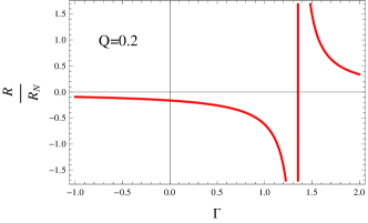
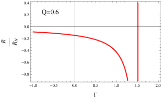
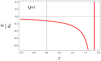
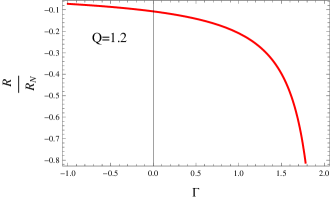
Figure 1: Plots of $\frac{R}{R_{N}}$ for dynamical stability/instability of homogeneous sphere corresponding to different values of Q.

When $\omega^{2}<0$, the perturbation diverges exponentially either by expansion or contraction which yields stellar dynamical instability. In the limit $\theta_{1}\rightarrow 0$, the condition for dynamical instability is

$$\Gamma-\frac{4}{21}\left(4Q^{2}+7\right)<\frac{14}{43}\theta_{1}^{2}=\frac{14}{43}\left[\frac{R^{2}}{a^{2}}-\frac{b^{2}}{R^{2}}\right].$$ (52)

In terms of inertial mass, this takes the form

$$R<\frac{14}{43\left[\Gamma-\frac{4}{21}\left(4Q^{2}+7\right)\right]}\left[\frac{2GM}{c^{2}}-\frac{GQ^{2}}{Rc^{4}}\right],$$ (53)

which can be written as

$$\frac{R}{R_{N}}<\frac{K}{\left[\Gamma-\frac{4}{21}\left(4Q^{2}+7\right)\right]},$$ (54)

where $K=\frac{14}{43}$ for the homogeneous sphere. This means that if $\Gamma$ exceeds $\frac{4}{3}+\frac{8Q^{2}}{21}$ by a small amount, the dynamical instability can be prevented till the mass contracts to the RN radius. If the radius of gaseous mass is greater than $R_{N}$, it remains stable. The ranges for instability of homogeneous spherical system are shown in Figure 1. Since the radius of stability is a factor of the RN radius, so the ratio $\frac{R}{R_{N}}$ should be greater than or equal to zero for physical results. We consider different values of charge and find that $0.1<Q<0.4$ and $\Gamma>1.5$ provide valid radii ranges for the stability of sphere. For $\Gamma<1.5$, we only have unstable radii along with un-physical region corresponding to $Q>0.4$. Also, we observe that the gaseous sphere becomes unstable forever with larger values of charge, i.e., $Q>1.2$. It is obvious from the graph that the radius of stability is greater than $R_{N}$ for $\Gamma>\frac{4}{3}+\frac{8Q^{2}}{21}$.

5.2 Relativistic Polytropic Model

In relativistic polytropic models, pressure and energy density can be expressed in terms of a single function $\Theta$ as [13]

$$p=p_{0}\Theta^{n+1},\quad\sigma=\sigma_{0}\Theta^{n},$$ (55)

where $p_{0}$ and $\sigma_{0}$ represent respective values at center and $n$ denotes the polytropic index. The polytropic models are the generalized form of the classical Lane-Emden equation which can be obtained from the equations of hydrostatic equilibrium. Let

$$\xi=\frac{r}{a},$$ (56)

where $a=\left(\frac{q(n+1)c^{4}}{4\pi G\sigma_{0}}\right)^{\frac{1}{2}}$ and $q=\frac{p_{0}}{\sigma_{0}}$. We can reduce Eqs.(13) and (14) to the pair of equations which express $\Theta$ as a function of $\xi$

$$\left(\frac{\xi^{2}}{1+q\Theta}-\frac{c^{2}Q^{2}q(n+1)}{32\pi G\sigma_{c}}\right)\left(1-\frac{2Vq(n+1)}{\xi}+\frac{Q^{2}Vq(n+1)}{\xi M}\right)\frac{d\Theta}{d\xi}$$

$$+V-\frac{Q^{2}V}{M}+q\Theta\frac{dV}{d\xi}=0,$$ (57)

$$\frac{dV}{d\xi}=\xi\Theta^{n}.$$ (58)

We assume pN approximation of the form

$$\Theta=\theta+q\Phi,$$ (59)

where $\Phi$ is an arbitrary function, $\theta$ represents classical Lane-Emden function and $q$ is treated as a small constant. Using Eqs.(57) and (58), the classical Lane-Emden equation becomes

$$\frac{d^{2}\theta}{d\xi^{2}}+\frac{2}{\xi}\frac{d\theta}{d\xi}+\left(1-\frac{Q^{2}}{M}\right)\theta^{n}=\frac{c^{2}Q^{2}}{32\pi G\sigma_{c}}.$$ (60)

Equation (43) in terms of $\Theta$ and $\xi$ takes the form

$$\frac{(a\omega)^{2}}{q}\int^{\xi_{1}}_{0}\Theta^{n}(1+q\Theta)\xi^{2}\eta^{2}e^{(3\lambda-\nu)/2}d\xi=2(n+1)q\int^{\xi_{1}}_{0}\Theta^{(2n+1)}(1+q\Theta)$$

$$\times\xi^{2}\eta^{2}e^{(3\lambda+\nu)/2}d\xi+4(n+1)\int^{\xi_{1}}_{0}\Theta^{n}\xi\eta^{2}e^{(\lambda+\nu)/2}\left(1-\frac{q\xi(n+1)}{4(1+q\Theta)}\right)d\xi$$

$$+\Gamma\int^{\xi_{1}}_{0}\frac{\Theta^{n+1}}{\xi^{2}}e^{(\lambda+3\nu)/2}\left(\frac{d}{d\xi}\left[\eta\xi^{2}e^{-\nu/2}\right]\right)^{2}d\xi+\left(\frac{1}{2\pi a^{3}}\right)^{2}\int^{\xi_{1}}_{0}\frac{e^{(\lambda+\nu)/2}}{\Theta^{n}(1+q\Theta)}$$

$$\times\left(\frac{\eta Q}{\xi^{4}}\right)^{2}\left[\frac{\xi}{2a}-Q^{2}\right]d\xi-\frac{1}{2\pi a^{3}}\int^{\xi_{1}}_{0}\frac{\eta^{2}}{\xi^{3}}e^{(\lambda+\nu)/2}\left[1+\frac{q(n+1)Q^{2}}{1+q\Theta}\frac{d\Theta}{d\xi}\right.$$

$$\left.-\frac{GQ_{0}^{2}}{\xi^{4}}\right]d\xi+\frac{1}{4\pi}\int^{\xi_{1}}_{0}\frac{\eta^{2}}{1+q\Theta}e^{(\lambda+\nu)/2}\frac{dQ^{2}}{d\xi}\left[q\frac{d\Theta}{d\xi}-\frac{1}{\Theta^{n}\left(a^{3}\xi^{3}\right)\frac{dQ^{2}}{d\xi}}\right]d\xi$$

$$-\frac{1}{8\pi a^{3}}\int^{\xi_{1}}_{0}\frac{\eta}{\xi^{2}}e^{(\lambda+\nu)}\frac{d^{2}}{dr^{2}}\left(Q^{2}\right)d\xi+\int^{\xi_{1}}_{0}\xi^{2}\eta e^{(\nu-\lambda)/2}\frac{d}{d\xi}\left[\frac{\beta Q_{0}\widetilde{Q}e^{\lambda_{0}}}{a\xi^{3}}\right]d\xi$$

$$+\frac{1}{4\pi a^{2}}\int^{\xi_{1}}_{0}\xi^{2}\eta e^{(\nu+\lambda)/2}\frac{d}{d\xi}\left(\frac{Q_{0}\delta Qe^{-\nu/2}}{\xi^{4}}\right)d\xi.$$ (61)

The pN approximation treats the effects of GR as first order corrections. We can write

$$\Gamma_{c}-\frac{4}{21}(4Q^{2}+7)=Cq,$$ (62)

$$R_{c}=\frac{K}{\Gamma_{c}-\frac{4}{21}(4Q^{2}+7)}\left[\frac{2GM}{c^{2}}-\frac{GQ^{2}}{Rc^{4}}\right],$$ (63)

where $C$ and $K$ are constants depending on density distribution. The pN approximation yields

$$e^{-\lambda}=1+2q(1+n)\xi\frac{d\theta}{d\xi}-\frac{GQ^{2}(1+n)q}{M}\frac{d\theta}{d\xi},$$ (64)

$$e^{\nu}=1-2q(1+n)[\theta+\xi_{1}|\tilde{\theta}_{1}|]+\frac{Q^{2}(1+n)q|\tilde{\theta}_{1}|}{M},$$ (65)

where $|\tilde{\theta}_{1}|=-\left(d\theta/d\xi\right)_{\xi=\xi_{1}}$. Using the relations of $p_{c}$ and $\sigma_{c}$ for polytropes in terms of $M$, $Q$ and $R$, it follows that

$$q=\frac{1}{2(n+1)\xi_{1}|\tilde{\theta}_{1}|}\left[\frac{2GM}{Rc^{2}}-\frac{GQ^{2}}{R^{2}c^{4}}\right].$$ (66)

We calculate $\Gamma$ with different values of $Q$ for the emergence of dynamical instability. The numerical values of $\Gamma$ for the polytropes of index 3 are given in Table 2. Similarly, the constants $C$ and $K$ for polytropes are given by the relation

$$K=\frac{C}{2(n+1)\xi_{1}|\tilde{\theta}_{1}|}.$$ (67)

Table 2: Adiabatic Index with Different Values of Charge for Dynamical Instability of Polytropes with Index 3
$q$ $\Gamma_{c}$ for $Q=0.2$ $\Gamma_{c}$ for $Q=0.4$ $\Gamma_{c}$ for $Q=0.6$ $0.015$ $1.3500$ 1.3593 1.4715 $0.040$ 1.3527 1.3983 1.4744 $0.1$ 1.3586 1.4043 1.4805 $0.2$ 1.3686 1.4143 1.4905 $0.5$ 1.3953 1.4440 1.5204

In order to determine the radii from Eq.(63), we need to calculate $K$ whose value depends upon the polytropic index, Lane-Emden function and charge. Different polytropic indices lead to different stellar structures such that the configurations with $n<5$ are considered to be realistic stars [17]. For $n=0$, we solve the Lane-Emden equation analytically corresponding to different values of $Q$ and find the values of $\theta$ but we solve this equation numerically for $n=2,3,4$ as shown in Figures 2-3. The values of constants $C$ and $K$ for $n=0$ are given in Table 3. We see that the values of $K$ decrease gradually by increasing the value of charge.

Table 3: Values of Constants $C$ and $K$ with Different Values of Charge for Polytropes of Index $0$
$C$ $K$ for $Q=0.2$ $K$ for $Q=0.4$ $K$ for $Q=0.6$ $0.243$ 0.6458 0.6372 0.576 $0.826$ $2.1953$ 2.1662 1.9608 $1.205$ 3.2034 3.161 2.8612 $1.8095$ 4.809 4.745 4.296

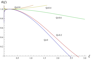
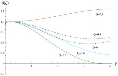
Figure 2: Plots of classical Lane-Emden function for polytropes of index $n=1,2$ corresponding to different values of charge.

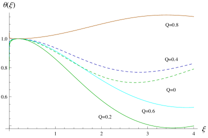
Figure 3: Plots of classical Lane-Emden function for $n=3$ corresponding to different values of charge.

Inserting the values of $e^{\nu}$ and $e^{-\lambda}$ in Eq.(61) and neglecting second as well as higher order terms in $q$, we obtain

$$\frac{(a\omega)^{2}}{q}\left\{\int^{\xi_{1}}_{0}\theta^{n}\xi^{2}\eta^{2}d\xi+\int^{\xi_{1}}_{0}H(\xi)\theta^{n-1}\xi^{2}\eta^{2}d\xi\right\}=\Gamma q(n+1)\int^{\xi_{1}}_{0}\frac{\theta^{n+1}}{\xi^{2}}$$

$$\times\left\{\left(\frac{GQ^{2}}{2M}-\xi\right)+3|\tilde{\theta}_{1}|\left(\frac{Q^{2}}{2M}-\xi_{1}\right)-3\theta\right\}\left[\frac{d}{d\xi}(\xi^{2}\eta)\right]^{2}d\xi+\Gamma\int^{\xi_{1}}_{0}H(\xi)$$

$$\times\frac{\theta^{n+1}}{\xi^{2}}\left\{\frac{d}{d\xi}\left(\xi^{2}\eta\right)\right\}^{2}d\xi+q(n+1)\int^{\xi_{1}}_{0}I(\xi)\theta^{n-1}\xi\eta^{2}d\xi+q(n+1)\int^{\xi_{1}}_{0}\frac{d\theta}{d\xi}$$

$$\times\left[\left(\frac{GQ^{2}}{2M}-\xi\right)+|\tilde{\theta}_{1}|\left(\frac{Q^{2}}{2M}-\xi_{1}\right)-\theta\right]Y(\xi)d\xi+q(n+1)\int^{\xi_{1}}_{0}\theta^{n+1}\xi^{2}\eta^{2}$$

$$\times Z(\xi)d\xi+\frac{1}{(2\pi)^{2}}\int^{\xi_{1}}_{0}\frac{\eta^{2}Q^{2}}{(a^{3}\xi^{2})^{3}}\left[\frac{\xi}{2a}-Q^{2}\right]d\xi-\frac{1}{8\pi}\int^{\xi_{1}}_{0}\frac{\eta}{a^{3}\xi^{2}}\frac{d^{2}}{d\xi^{2}}(Q^{2})d\xi$$

$$-\frac{1}{2\pi}\int^{\xi_{1}}_{0}\frac{GQ^{2}}{a^{3}\xi^{4}}d\xi+\int^{\xi_{1}}_{0}\xi^{2}\eta\frac{d}{d\xi}\left(\frac{\beta Q_{0}\widetilde{Q}}{a\xi^{3}}\right)d\xi,$$ (68)

where

$$H(\xi) = 2\theta^{2}(n+2)+3(n+1)\left(\frac{GQ^{2}}{2M}-\xi\right)\frac{d\theta}{d\xi}+\left(2\xi_{1}-\frac{Q^{2}}{2M}\right)$$ (69)

$$\times (n+1)|\tilde{\theta}_{1}|,$$

$$I(\xi) = -4\theta(n+1)\frac{d\theta}{d\xi}\left[-\xi\frac{d\theta}{d\xi}-\theta-\xi|\tilde{\theta}_{1}|+\frac{Q^{2}}{2M}\left(G\frac{d\theta}{d\xi}+|\tilde{\theta}_{1}|\right)\right],$$ (70)

$$Y(\xi) = \frac{\eta^{2}Q^{2}}{2\pi^{2}(a^{3}\xi^{2})^{2}}\left(\frac{\xi}{2a}-Q^{2}\right)-\frac{\eta^{2}}{2\pi a^{3}\xi^{3}}+\frac{GQ_{0}^{2}}{2\pi a^{3}\xi^{4}}-\frac{\eta}{4\pi a^{3}\xi^{2}}$$ (71)

$$\times \frac{d^{2}}{d\xi^{2}}(Q^{2})+\xi^{2}\eta\frac{d}{d\xi}\left\{\frac{\beta Q_{0}\widetilde{Q}}{a\xi^{3}}+\eta\xi^{2}\frac{d}{d\xi}\left(\frac{Q_{0}\delta Q}{\xi^{4}}\right)\right\},$$

$$Z(\xi) = 3\theta\left(\frac{Q^{2}}{2M}-\xi\right)\frac{d\theta}{d\xi}+\theta|\tilde{\theta}_{1}|\left(\frac{Q^{2}}{2M}-2\xi_{1}\right)-2\theta^{2}.$$ (72)

In pN approximation, we are interested to find the condition for marginal stability of polytropic configuration by taking $\eta=\xi$ and $\omega^{2}=0$ so that Eq.(68) takes the form

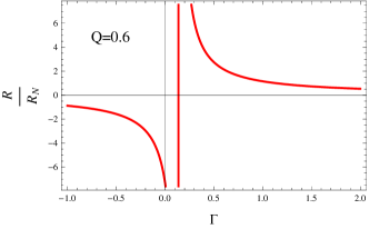
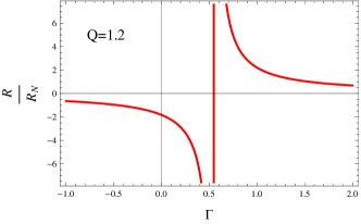
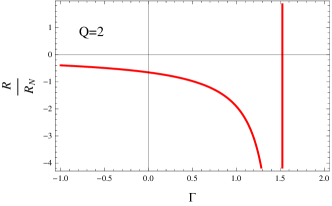
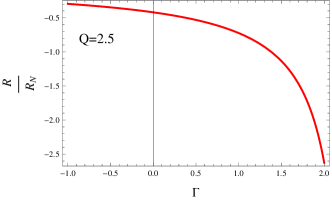
Figure 4: Plots for radii of stability/instability corresponding to $n=1$ and different values of charge.

$$9\left(\Gamma-\frac{4}{3}-\frac{8Q^{2}}{21}\right)\int^{\xi_{1}}_{0}\theta^{n+1}\xi^{2}d\xi+q(n+1)\left[3\int^{\xi_{1}}_{0}\theta^{n}Y(\xi)\widetilde{Y}(\xi)d\xi\right.$$

$$\left.+\int^{\xi_{1}}_{0}\theta^{n-1}I(\xi)\xi^{3}d\xi+\int^{\xi_{1}}_{0}\theta^{n+1}\xi^{4}Z(\xi)d\xi\right]+\frac{1}{8\pi}\int^{\xi_{1}}_{0}\frac{\widetilde{Z}(\xi)}{a^{3}\xi^{3}}d\xi$$

$$+\int^{\xi_{1}}_{0}\xi^{3}\frac{d}{d\xi}\left(\frac{\beta Q\widetilde{Q}}{a\xi^{3}}\right)d\xi=0,$$

(73)

with

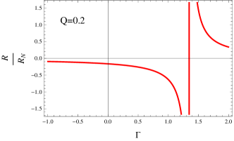
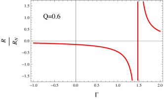
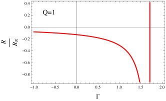
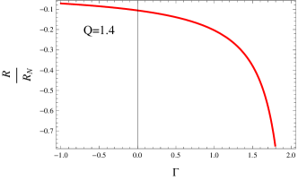
Figure 5: Plots for radii of stability/instability corresponding to $n=2$ and different values of charge.

$$\widetilde{Y}(\xi) = \left(3\Gamma\xi^{2}\theta+\theta^{-n}\right)\left\{\frac{d\theta}{d\xi}\left(\frac{GQ^{2}}{2M}-\xi\right)+3|\tilde{\theta}_{1}|\left(\frac{Q^{2}}{2M}-\xi_{1}\right)-3\theta\right\},$$

$$\widetilde{Z}(\xi) = 4Q^{2}\left(G+\frac{\xi}{2M}-Q^{2}\right)-\xi^{3}\left(1+\frac{d^{2}}{d\xi^{2}}(Q^{2})\right).$$ (75)

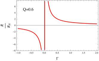
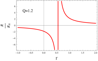
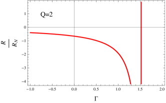
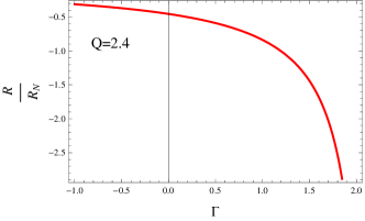
Figure 6: Plots for radii of stability/instability corresponding to $n=3$ and different values of charge.

In pN limit, the dynamical stability will require that $\Gamma>\Gamma_{c}=\frac{4}{3}+\frac{8Q^{2}}{21}+\epsilon$, where $\epsilon$ is a small quantity depending on $q$. To check the conditions for marginal stability as well as dynamical instability, we calculate values of $K$ and plot different radii corresponding to polytropic indices $n=1,2,3$ as shown in Figures 4-6. It is found that $K$ attains negative values for $n=1,2,3$, so we take both positive and negative values of $\Gamma$ to obtain physically viable values of radii. Figures 4 and 5 show viable radii for $\Gamma>\frac{4}{3}+\frac{8Q^{2}}{21}$ corresponding to $n=1,2$. For $n=1$, we find that radii of stability along with non-physical region appear for $Q=0.6$ and positive values of $\Gamma$ while negative values of $\Gamma$ show the emergence of instability. The region of instability gets larger by increasing $Q$ for both positive and negative values of $\Gamma$ and the radii of marginal stability vanishes for $Q=2$. We observe that the the corresponding polytropic model becomes unstable for $Q>2.4$ (Figure 4).

For $n=2$, we analyze stable radii for $1.5<\Gamma<2$ and unstable radii for small values of $\Gamma$ (both positive and negative) corresponding to $Q<1$. The stability radius tends to decrease which leads to unstable region for $Q=1$. We find that the non-physical region disappears and the polytropic model will remain unstable forever with $Q\geq 1.4$ (Figure 5). For $n=3$, we have viable ranges for radii with $0<\Gamma<2$, i.e., $\Gamma$ can be less than $\frac{4}{3}+\frac{8Q^{2}}{21}$ for stable stellar structures (Figure 6). We find both stable and unstable radii for polytropic model with $0.1<Q<2$ which changes to unstable radii for $Q\geq 2$. The dynamical instability occurs when gaseous mass contracts to $R_{N}$.

6 Conclusions

This paper is devoted to investigate the role of electric charge on dynamical stability of spherical gaseous masses under radial oscillations. We have perturbed the system using Eulerian and Lagrangian radial perturbations to obtain linearized dynamical equations as well as perturbed pressure. This perturbed pressure in terms of adiabatic index is found using conservation of baryon number. The variational principle has been applied to the perturbed dynamical equations to formulate conditions of dynamical instability. We have also discussed conditions for dynamical instability of homogeneous sphere and relativistic polytropes in Newtonian as well as pN regimes.

We have found the values of adiabatic index $\Gamma$ as well as radii for marginal stability of homogeneous sphere (Table 1). It turns out that $\Gamma$ takes finite positive values less or greater than $\frac{4}{3}+\frac{8Q^{2}}{21}$ corresponding to different values of charge at Newtonian limit. The radius $\frac{R}{R_{N}}$ approaches to infinity for $\Gamma<0$ which leads to expansion rather than collapse. In pN limit, the dynamical instability occurs if $\Gamma$ exceeds $\frac{4}{3}+\frac{8Q^{2}}{21}$ by a small quantity and the gaseous mass is contracted to RN radius. We have found that $0.1<Q<0.4$ and $\Gamma>1.5$ provide valid radii ranges for stability of sphere. It turns out that only unstable radii exist corresponding to $Q>1.2$.

We have also discussed the stability/instability conditions for relativistic polytropic models of indices $0,1,2$ and $3$. For $n=3$, we have evaluated different values of $\Gamma$ for dynamical instability of polytropes and found that $\Gamma>\frac{4}{3}+\frac{8Q^{2}}{21}$ (Table 2). In order to discuss realistic models, we have evaluated radius of instability for different polytropic structures. We have also calculated the values of $C$ and $K$ for $n=0$ (Table 3), which show that $K$ decreases gradually by increasing the values of charge. For $n=1,2$, we have viable radii corresponding to $\Gamma>\frac{4}{3}+\frac{8Q^{2}}{21}$. For $n=1$, we have found that radii of stability along with non-physical region exist for $Q=0.6$ and $\Gamma>0$ while negative values of $\Gamma$ show the emergence of instability. The region of instability increases by increasing $Q$ for both positive and negative values of $\Gamma$ and we find only unstable radii for $Q>2.4$. For $n=2$, we have found both stable and unstable radii for $1.5<\Gamma<2$. The stability radius tends to decrease gradually which leads to unstable region for $Q=1.4$. It is seen that $\Gamma$ can be less than $\frac{4}{3}+\frac{8Q^{2}}{21}$ for $n=3$. We have analyzed both stable and unstable radii for polytropic model with $0.1<Q<2$ which changes to unstable radii for $Q\geq 2$.

It is found that the dynamical instability occurs when the mass of polytropic configuration approaches to the RN radius limit. We observe that inclusion of charge in the gaseous sphere has significant effects as compared to the analysis [2]. For charged homogeneous sphere, the system becomes stable for both negative as well a as positive values of adiabatic index, while it remains stable for $\Gamma>\frac{4}{3}$ without charge system [2]. For the charged polytropes with $n=1,2,3$, $\Gamma$ can take both positive as well as negative values while $K$ becomes negative. We also see that the radius of instability of polytropes ($n=3$) for RN case is greater than that of the Schwarzschild limit showing that RN polytropes for $n=3$ are more stable. Finally, we conclude that the presence of charge has substantial role in the emergence of instability of gaseous sphere.

References

- [1] Ayal, S. et al.: Astrophys. J. 550(2001)846; Marek, A. et al.: Astron. Astrophys. 445(2006)273.
- [2] Chandrasekhar, S.: Astrophys. J. 140(1964)417.
- [3] Chandrasekhar, S.: Astrophys. J. 142(1965)1519.
- [4] Herrera, L., Le Denmat, G. and Santos, N.O.: Mon. Not. R. Astron. Soc. 237(1989)257.
- [5] Chan, R., Herrera, L. and Santos, N.O.: Mon. Not. R. Astron. Soc. 267(1994)637; Nunez, L.A., Hernandez, H. and Abreu, H.: Class. Quantum Grav. 24(2007)4631; Sharif, M. and Azam, M.: Gen. Relativ. Gravit. 44(2012)1181.
- [6] Rosseland, S.: Mon. Not. R. Astron. Soc. 84(1924)720.
- [7] Eddington, A.: Internal Constitution of the Stars (Cambridge University Press, 1926).
- [8] Stettner, R.: Ann. Phys. 80(1973)212.
- [9] Glazer, I.: Ann. Phys. 101(1976)594.
- [10] Ghezzi, C.R.: Phys. Rev. D 72(2005)104017.
- [11] Sharif, M. and Azam, M.: J. Cosmol. Astropart. Phys. 02(2012)043; Sharif, M. and Bhatti, M.Z.: J. Cosmol. Astropart. Phys. 10(2013)056.
- [12] Chandrasekhar, S.: An Introduction to the Study of Stellar Structure (University of Chicago, 1939).
- [13] Tooper. R.F.: Astrophys. J. 140(1966)434.
- [14] Ray, S. et al.: Braz. J. Phys. 34(2004)310; Fronsdal, C.: Lett. Mathem. Phys. 82(2007)255.
- [15] Herrera, L. and Barreto, W.: Phys. Rev. D 88(2013)084022.
- [16] Breysse, P.C., Kamionkowski, M. and Benson, A.: Mon. Not. R. Astron. Soc. 437(2014)2675.
- [17] Horedt, G.P.: Polytropes: Applications in Astrophysics and Related Fields (Kluwer Academic, 2004).