Cascades in interdependent flow networks

Abstract

In this manuscript, we investigate the abrupt breakdown behavior of coupled distribution grids under load growth. This scenario mimics the ever-increasing customer demand and the foreseen introduction of energy hubs interconnecting the different energy vectors. We extend an analytical model of cascading behavior due to line overloads to the case of interdependent networks and find evidence of first order transitions due to the long-range nature of the flows. Our results indicate that the foreseen increase in the couplings between the grids has two competing effects: on the one hand, it increases the safety region where grids can operate without withstanding systemic failures; on the other hand, it increases the possibility of a joint systems’ failure.

url]https://sites.google.com/site/antonioscalaphys/

1 Introduction

Physical Networked Infrastructures ($PNI$s) such as power, gas or water distribution are at the heart of the functioning of our society; they are very well engineered systems designed to be at least $N-1$ robust – i.e., they should be resilient to the loss of a single component via automatic or human guided interventions. The constantly growing size of $PNI$s has increased the possibility of multiple failures which escape the $N-1$ criteria; however, implementing robustness to any sequence of $k$ failures ($N-k$ robustness) requires an exponentially growing effort in means and investments. In general, since $PNI$s can be considered to be aggregations of a large number of simple units, they are expected to exhibit emergent behaviour, i.e. they show as a whole additional complexity beyond what is dictated by the simple sum of its parts [1].

A general problem of $PNI$s are cascading failures, i.e. events characterized by the propagation and amplification of a small number of initial failures that, due to non-linearity of the system, assume system-wide extent. This is true even for systems described by linear equations, since most failures (like breaking a pipe or tripping a line) correspond to discontinuous variations of the system parameters, i.e. are a strong non-linear event. This is a typical example of emergent behavior leading to one of the most important challenges in a network-centric word, i.e. systemic risk. An example of systemic risk in $PNI$s are the occurrence of blackout in one of the most developed and sophisticated system, i.e. power networks. It is important to notice that if such large outages were intrinsically due to an emergent behaviour of the electric power systems, increasing the accuracy of power systems’ simulation would not necessarily lead to better predictions of black-outs.

Power grids can be considered an example of complex networks[2]and hence cascading failures in complex networks [3] is field with important overlaps with system engineering and critical infrastructures protection; however, most of the cascading model are based on local rules that are not appropriate to describe systems like power grids [4] that, due to long range interactions, require a different approach [5, 6].

Another import issue is increasing interdependent among critical infrastructures[7]; seminal papers have pointed out the possibility of the occurrence of catastrophic cascades across interdependent networks [8, 9]. However, there is still room for increasing the realism of such models[10], especially in the case of electric grids or gas pipelines. In this paper we move a preliminary step in such direction, trying to capture the systemic effect for coupled networks with long range interactions.

To highlight the possibility of emergent behavior, we will first abstract $PNI$s in order to understand the basic mechanisms that could drive systemic failures; in particular, we will consider finite capacity networks where a commodity (a scalar quantity) is produced at source nodes, consumed at load nodes and distributed as a Kirchoff flow (e.g. fluxes are conserved). For such systems, we will first introduce a simplified model that is amenable of a self-consistent analytical solution. Subsequently, we will extended such model to the case of several coupled networks and study the cascading behavior under increasing stress (i.e. increasing flow magnitudes).

In section 2, we develop our simplified model of overload cascades first in isolated (sec. 2.2) and coupled systems (sec. 2.3). In particular, in subsection 2.1, we introduce the concept of flow network with a finite capacity and relate conservation laws to Kirchoff’s equations and to the presence of long range correlation. To account for such correlations, in subsection 2.2 we introduce a mean field model for the cascade failures of flow networks; in subsection 2.3, we extend the model to the case of several interacting systems. Finally, in section 3 we discuss and summarize our results.

2 Model

2.1 Flow networks

Let’s consider a network $G=\left(\mathcal{V},\mathcal{E},\mathbf{c}\right)$ where $\mathcal{V}=\left\{1\leq i\leq\left|\mathcal{V}\right|\right\}$ is the node set, $\mathcal{E}\subseteq\mathcal{V}\times\mathcal{V}$ is the set of edges and $\mathbf{c}=\{c_{\left(i,,j\right)}\}$ is the vector characterizing the capacities of the edges $\left(i,j\right)$. We associate to the nodes a vector $\mathbf{p}=\{p_{i}\}$ that characterize the production ($p_{i}>0$) or the consumption ($p_{i}<0$) of a commodity. We further assume that there are no losses in the network (i.e. $\sum_{i}p_{i}=0$); hence, the total load on the network is

$$L={\displaystyle\sum_{i:p_{i}>0}}p_{i}$$

The distribution of the commodity is described by the fluxes $\mathbf{f}=\{f_{\left(i,j\right)}\}$ on the edges $\left(i,j\right)\in\mathcal{E}$ that are supposed to respect Kirchoff equations, i.e.

$$\sum_{j}f_{\left(i,j\right)}=p_{i}$$ (1)

The relation among fluxes and demand/load is described by constitutive equations

$$\mathbf{f}=F(\mathbf{p},G)$$ (2)

where in general eq.2 is non-linear but satisfies eq.1.

The finite capacity $c_{\left(i,j\right)}$ constrains the maximum flux on link $\left(i,j\right)$

$$|f_{\left(i,j\right)}|<c_{\left(i,j\right)}$$ (3)

above which the link will cease functioning. As an example, power lines are tripped (disconnected) when power flow goes beyond a certain threshold. Since flows will redistribute after a link failure, it could happen that other lines get above their flow threshold and hence consequently fail, eventually leading to a cascade of failures. A typical algorithm to calculate the consequences of an initial set of line failures $\mathcal{F}^{0}=\{(ij)\,\,$failed$\}$ is the alg.1.

Algorithm 1 Network cascading

  Set initial failures $\mathcal{F}^{0}$

  $t\leftarrow 0$

  repeat

     $t\leftarrow t+1$

     Calculate flows $\mathbf{f}^{t}\leftarrow F(\mathbf{p},G|\mathcal{F}^{t-1})$

     Calculate new failures $\Delta\mathcal{F}^{t}\leftarrow\{(ij):|f_{ij}^{t}|>c_{ij}\}$

     $\mathcal{F}^{t}\leftarrow\mathcal{F}^{t-1}\cup\Delta\mathcal{F}^{t}$

  until $\Delta\mathcal{F}^{t}\equiv\emptyset$

Here $F(\mathbf{p},G|\mathcal{F})$ calculates the flows subject to the constrains that flows are zero in the failure set of edges $(i,j)\in\mathcal{F}$.

To develop a general model that helps us understanding the class of failures that can affect Kirchoff-like flow networks, let’s start from rewriting eq.1 in matrix form

$$\mathcal{B^{T}}\mathbf{f}=\mathbf{p}$$ (4)

using the incidence matrix $B$ that associates to each link $\left(i,j\right)$ its nodes $i$ and $j$ and vice-versa. $B$ is an $\left|\mathcal{V}\right|\times\left|\mathcal{E}\right|$ matrix where each column corresponds to an edge $\left(i,j\right)$; its columns are zero-sum and the only two non-zero elements have modulus $1$ and are on the $i^{th}$ and on the $j^{th}$ row.

The matrix $B$ is related to the Laplacian $B^{T}B$ of the system; in particular, it shares the same right eigenvalues and the same spectrum (up to a squaring operations); hence, it is a long-range operator since perturbation on a node of the system can be reflected on nodes far away on the network [5, 6].

2.2 Mean field model for cascades on a single network

Due to the long range nature of Kirchoff’s equations, to understand the qualitative behavior of such networks we can resort to a mean field model of flow networks where one assumes that when a link fails, its flow is re-distributed equally among all other links. Subsequently, the lines above their threshold would trip again, their flows would be re-distributed and so on, up to convergence; recalling that $L$ is the total load of the system and assuming the each link $\left(i,j\right)$ has an initial flux $f=L/\left|\mathcal{E}\right|$, we can describe such a model by alg.2. Such model, introduced in [5], is akin to the fiber-bundle model [11, 12] and has been considered in more details in [13, 14] for the case of a single system. While similar in spirit to the CASCADE model for black-outs [15, 16], it yelds different results since it does not describe the statistic of the cascades in power systems but concentrates on the order of the transition in a single system.

Algorithm 2 Mean Field cascading

  $t\leftarrow 0$

  $F^{t}\leftarrow 0$ initial number of failed links

  repeat

     $t\leftarrow t+1$

     $M\leftarrow\left|\mathcal{E}\right|-F^{t-1}$ number of working links

     $l\leftarrow L/M$ average flux on the working links

     $F^{t}\leftarrow\left|\left\{(ij):l>c_{(ij)}\right\}\right|$

  until $F^{t}=F^{t-1}$

Such algorithm can be cast in the form of a single equation in the case where the system is composed by a large number of elements with capacity $c$. In fact, in such limit we can describe the links’ population by the probability distribution function $p(c)$ of their capacities. Indicating with $M=\left|\mathcal{E}\right|$ the initial number of links, we see that if we apply an overall load $L$ to the system, all the links will be initially subject to a flow $l^{0}=L/M$. Thus, a fraction of links $f^{1}=\int_{0}^{L/M}p\left(c\right)dc$ would immediately fail, since their thresholds are lower than the flux $l$ they should sustain. After the first stage of a cascade, there will be $M^{1}=(1-f^{1})M$ surviving links and the new load per link is $l^{1}=L/M^{1}$. The following cascade’s stages follow analogously; we can thus write the mean field equations for the $\left(t+1\right)^{th}$ stage of the cascade:

$$f^{t+1}=P\left(\frac{l}{1-f^{t}}\right)$$ (5)

where $l=L/M$ is the initial load per link and $P\left(x\right)=\int_{0}^{x}p\left(c\right)dc$ is the cumulative distribution function of link capacities; the initial conditions are $f^{t=0}=0$. The fix-point $f^{*}$ of eq.5 satisfies the equation

$$f^{*}=P\left(\frac{l}{1-f^{*}}\right)$$ (6)

and represents the total fraction of links broken at the end of the cascading stages [5, 6].

The behavior of $f^{*}$ depends on the functional form of $p\left(c\right)$. In particular, following[17] we can define $\pi(c)=1-P(c)$ and $x=l^{-1}(1-f)$ and we have that

$$f=\int_{0}^{1/x}p\left(c\right)dc=1-\pi\left(\frac{1}{x}\right)$$ (7)

so that we can rewrite eq.(5) as

$$lx^{t+1}=\pi\left(\frac{1}{x^{t}}\right)$$ (8)

Equation (8) has a trivial fix-point $x^{*}=0$ (representing a total breakdown of the system) since $\pi\left(\infty\right)=0$. Such fix-point is unstable for $l\to 0$ and becomes stable for $l>\partial_{x}\pi(x^{-1})|_{x\to 0}$. We notice that if $P\left(c\right)$ does not change convexity (i.e. has no bumps) and the transition is first order, the system will breakdown directly to the total collapsed state $f=1$.

In general, the behavior of the fix-point $x^{*}$ depends on the tail of the distribution $p(c)$ and is known to present a first order transition for a wide family of curves [17].

Depending on the functional form of $p\left(c\right)$, eq.(6) could sometimes be solved analytically. Otherwise, the fix-point of eq. (6) can be solved numerically either by iterating the eq. (5) or by finding the zeros of eq.(6) by Newton-Raphson iterations.

Notice that, if the system is long range, modelling cascade via homogeneous load redistribution allows to capture the order of the transition even when it gives not an accurate prediction of the actual location of the transition point. An example of such accordance for the case of power networks is given in [5, 6], where both synthetic networks, realistic networks and mean-field systems show a first order transition.

2.3 Mean field model for interacting cascades

Commodities are defined substitutable when they can be used for the same aim; when commodities are substitutable, they can expressed in the same units. An example of such commodities are electricity and gas, since both can be used for domestic heating. Hence, an increase on the cost of the gas (as the one that has been recently experienced by Ukraine) could induce stress on the electric network of the country since most customer will possibly switch to the cheaper energy vector . To take account for such effects, we will extend the model described by eq.(5) to the case of several coupled systems that transport substitutable commodities.

We will consider $n$ coupled systems assuming that when a system $a$ is subject to some failures, it sheds a fraction $T_{a\to b}$ of the induced flow increase on system $b$. In other words, after failure system $a$ decreases its stress by a quantity $l_{a}f_{a}{\displaystyle\sum_{b\neq a}}T_{a\to b}$ by increasing the load of all other systems $b\neq a$ by $l_{a}f_{a}T_{a\to b}$. Thus, the $n$ coupled systems are described by a set of $n$ equations of the form of eq.(5)

$$f_{a}^{t+1}=P_{a}\left(\frac{\tilde{l_{a}^{t}}}{1-f_{a}^{t}}\right)$$ (9)

where $\tilde{l_{a}^{t}}$ is the load per link experimented by system $a$ in the $t^{th}$ stage of the cascade and $P_{a}\left(x\right)=\int_{0}^{x}p_{a}\left(x\right)dx$ is the cumulative of the probability distribution function $p_{a}\left(x\right)$ for the capacities of the $a^{th}$ system. Equations (9) are not independent, since the systems’ coupling is reflected by the dependence of $\tilde{l_{a}^{t}}$ on the fractions $f_{b}^{t}$ of failed links in all the other systems, i.e.

$$\tilde{l_{a}^{t}}=l_{a}(1-f_{a}^{t}\sum_{b}T_{a\to b})+\sum_{b}T_{b\to a}l_{b}f_{b}^{t}=l_{a}+\sum_{b}\mathcal{L}_{ab}l_{b}f_{b}^{t}$$ (10)

where $\mathcal{L}_{ab}=(1-\delta_{ab})T_{b\to a}+\delta_{ab}\sum_{b}T_{a\to b}$ has the form of a Laplacian operator. Thus, the full equations for $n$ coupled systems are

$$f_{a}^{t+1}=P_{a}\left(\frac{l_{a}+\sum_{b}\mathcal{L}_{ab}l_{b}f_{b}^{t}}{1-f_{a}^{t}}\right)$$ (11)

.

For simplicity, from now on we will consider the case of two identical systems with a uniform distribution of link capacities. Notice that for a single system the transition is first order unless the probability distribution of the capacities is a power-law [17] – an event that is not realistic for real world flow networks. Since the functional form of $P(.)$ is easy to recover for a uniform distribution, we can solve the fix-point of eq.(11) numerically by iterating the equations up to convergence; an alternative methodology would be using Newton-Raphson algorithms. We show in fig.(1) the cascading behavior of two coupled systems; we observe that – as in the single system case – transitions are in the form of abrupt jumps, i.e. are first order. Let’s rewrite eq.(11) in the case of symmetric couplings $T_{1\to 2}=T_{2\to 1}=1$ and same probability distribution for the capacities

$$\left\{\begin{array}[]{c}f_{1}^{t+1}=P\left(\frac{l_{1}}{1-f_{1}^{t}}\left[1-T\left(f_{1}-\frac{l_{2}}{l_{1}}f_{2}\right)\right]\right)\\ f_{2}^{t+1}=P\left(\frac{l_{1}}{1-f_{2}^{t}}\left[1-T\left(f_{2}-\frac{l_{1}}{l_{2}}f_{1}\right)\right]\right)\end{array}\right.$$ (12)

If the two systems described by eq.(12) are stressed at the same pace (i.e. $l_{1}=l_{2}=l/2$), we get the case

$$\left\{\begin{array}[]{c}f_{1}^{t+1}=P\left(\frac{l}{1-f_{1}^{t}}\left[1-T\Delta f_{12}\right]\right)\\ f_{2}^{t+1}=P\left(\frac{l}{1-f_{2}^{t}}\left[1+T\Delta f_{12}\right]\right)\end{array}\right.$$

; from the symmetric solution $\Delta f_{12}=0$ we see that the breakdown of both systems happen at the same critical load as the uncoupled systems. Such situation is shown in the left panel of fig.(1).

In the general, only one of the systems will be the first one to break down (i.e. the fraction of broken links jumps to $f^{*}=1$): correspondingly, also the other systems will experience a jump in the number of broken links. Let’s consider the symmetric case described by equations (12) and suppose that $l_{1}>l_{2}$, so that system $1$ is the first to breakdown (i.e. $f_{1}^{*}=1$); hence, the equation for the fix-point of the second system becomes

$$f_{2}^{*}=P\left(\frac{l}{1-f_{2}^{*}}\left[1+T\left(1-f_{2}^{*}\right)\right]\right)=P\left(\frac{l^{+}}{1-f_{2}^{*}}\right)$$

i.e. the system behaves like a single system starting with a renormalized load $l^{+}=l\,\left[1+T\left(1-f_{2}^{*}\right)\right]>l$. Thus, if $l^{+}<l_{c}$ ( the critical value of eq.(5), system $2$ will break down at higher values of the stress. Such situation is shown in the right panel of fig.(1).

In fig.(2) we show the full phase diagrams of two coupled systems while varying the coupling among them. According to the initial loads, we can distinguish an area $S$ near the origin where the system is safe and three separate cascade regimes: $B_{1}$ and $B_{2}$, where either system $1$ or $2$ fails, and $B_{12}$ where both systems fail. We notice that, by increasing the coupling among the systems, both the area $S$ where the two systems are safe and the area $B_{12}$ where they fail together grow; accordingly, the areas $B_{i}$ where only one system fails shrink.

3 Discussion

We have introduced a model for cascade failures due to the redistribution of flows upon overload of link capacities. For such a model, we have developed a mean field approximation both for the case of a single network and for the case of coupled networks. Our model is inspired to a possible configuration for future power systems where network nodes the so-called energy hubs [18], i.e. points where several energy vectors converge and where energy demand/supply can be satisfied converting one kind of energy in another. Hubs condition, transform and deliver energy in order to cover consumer needs [19]. In such configurations, one can alleviate the stress on a network by using the flows of the the other energy vectors; on the other hand, transferring loads from a network to the other can trigger cascades that can eventually backfire.

By analyzing the case of two coupled systems and by varying the strength of the interactions among them, we have shown that at low stresses coupling has a beneficial effect since some of the loads are shed to the other systems, thus postponing the occurrence of cascading failures. On the other hand, with the introduction of couplings the region where not only one system fails but both systems fail together also increases. The higher the couplings, the more the two systems behave like a single one and the area where only a system has failed shrinks.

Our model also applies to the realistic scenario where existent grids gets connected to allow power to be delivered across states; such scenario has inspired the analysis of [9] that, even using an unrealistic model of power redistribution in electric grids, reaches conclusion that are similar to ours.

It is worth noting that while fault propagation models do predict a general lowering of the threshold for coupled systems [20], in the present model a beneficial effect due to the existence of the interdependent networks is observed for small enough overloads, while the expected cascading effects take place only for large initial disturbances. This picture is consistent with the observed phenomena for interdependent Electric Systems. Moreover the existence of interlinks among different networks may increase their synchronization capabilities [21].

References

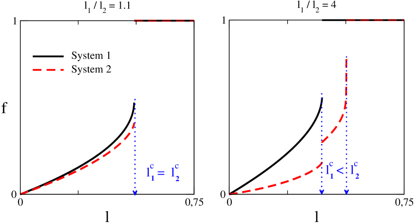
Figure 1: Behaviour of the number of failed nodes respect to the total stress $l=l_{1}+l_{2}$ of the systems. For simplicity, we present the case of two identical systems with a flat distribution of link capacities and symmetric couplings $T_{1\to 2}=T_{2\to 1}=0.5$. We show the result of increasing the total stress $l$ in the two systems along the lines $l_{1}/l_{2}=const$. Left panel: we show the case $l_{1}/l_{2}=1.1$ where both systems are subject to a similar stress while increasing $l$. In such case both system break down together at the same critical load $l_{1}^{c}=l_{2}^{c}$; in the region $l>l_{1}^{c}=l_{2}^{c}$ both systems have failed. Right panel: we show the case $l_{1}/l_{2}=4$ where when increasing $l$ system $1$ is more stressed than system $2$. In this case, the break down of system $1$ at the critical load $l_{1}^{c}$ induces a jump in the number of failures system $2$, but system $2$ is still able to sustain stress and will break down only at higher values of $l$. Respect to the $l_{1}\sim l_{2}$ case, there is now a region $l_{1}^{c}<l<l_{2}^{c}$ where only system $1$ has failed.

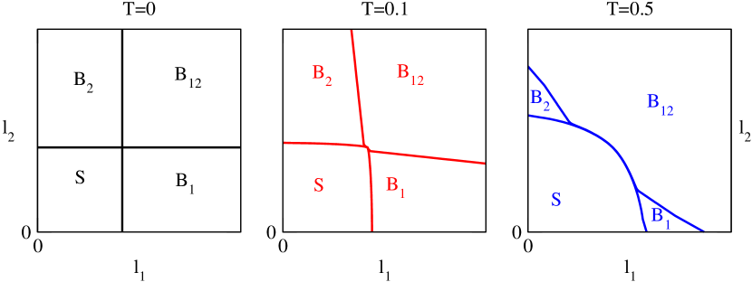
Figure 2: Phase diagrams of two identical coupled systems with symmetric interactions ($T_{1\to 2}=T_{2\to 1}=T$). The plane of initial loads $l_{1}$ and $l_{2}$ is separated in four different regions by critical transition lines. The labels $B_{i}$ ($i=1,2$) mark the areas where only system $i$ suffers systemic cascades ($f_{i}^{*}=1$,$f_{j\neq i}^{*}<1$), while the label $B_{12}$ marks the area where both systems suffer system wide cascades ($f_{1}^{*}=f_{2}^{*}=1$). The label $S$ marks the area near the origin where no systemic cascades occur. Left panel: the case $T=0$ corresponds to two uncoupled systems: thus, each system suffers systemic failure at $l_{i}>l^{c}$ (where $l^{c}$ is the critical load for an isolated system); both systems have failed in the $B_{12}$ area corresponding to the quadrant $(l_{1}>l^{c},l_{2}>l^{c})$. Central panel, right panel: when couplings are introduced, each system is able to discharge stress on the other one and the area $S$ where both systems are safe increases. On the other hand, the area $B_{12}$ where both systems are in a failed state increases.

References

-
[1]
P. W. Anderson,
More is
different, Science 177 (4047) (1972) 393–396.
arXiv:http://www.sciencemag.org/content/177/4047/393.full.pdf, doi:10.1126/science.177.4047.393.
URL http://www.sciencemag.org/content/177/4047/393.short -
[2]
G. A. Pagani, M. Aiello,
The
power grid as a complex network: A survey, Physica A: Statistical Mechanics
and its Applications 392 (11) (2013) 2688 – 2700.
doi:http://dx.doi.org/10.1016/j.physa.2013.01.023.
URL http://www.sciencedirect.com/science/article/pii/S0378437113000575 - [3] P. Crucitti, V. Latora, M. Marchiori, Model for cascading failures in complex networks, Phys. Rev. E 69 (2004) 045104. doi:doi:10.1103/PhysRevE.69.045104.
-
[4]
P. Hines, E. Cotilla-Sanchez, S. Blumsack,
Do
topological models provide good information about electricity infrastructure
vulnerability?, Chaos 20 (3) (2010) –.
doi:http://dx.doi.org/10.1063/1.3489887.
URL http://scitation.aip.org/content/aip/journal/chaos/20/3/10.1063/1.3489887 -
[5]
S. Pahwa, C. Scoglio, A. Scala,
Abruptness of cascade failures in
power grids, Sci. Rep. 4 (2014) –.
URL http://dx.doi.org/10.1038/srep03694 - [6] A. Scala, S. Pahwa, C. Scoglio, Cascade failures and distributed generation in power grids, Int. J. Critical Infrastructures 11 (1) (2015) 27–35.
- [7] S. M. Rinaldi, J. P. Peerenboom, T. K. Kelly, Identifying, understanding and analyzing critical infrastructure interdependencies, Ieee Contr Syst Mag 21 (6) (2001) 11–25.
- [8] S. V. Buldyrev, R. Parshani, G. Paul, H. E. Stanley, S. Havlin, Catastrophic cascade of failures in interdependent networks, Nature 464 (7291) (2010) 1025–1028.
- [9] C. D. Brummitt, R. M. D’Souza, E. A. Leicht, Suppressing cascades of load in interdependent networks, P Natl Acad Sci Usa 109 (12) (2012) E680–E689. doi:doi:10.1073/pnas.1110586109.
-
[10]
G. D’Agostino, A. Scala,
Networks of
Networks: The Last Frontier of Complexity, Understanding Complex Systems,
Springer International Publishing, 2014.
doi:10.1007/978-3-319-03518-5.
URL http://link.springer.com/book/10.1007%2F978-3-319-03518-5 - [11] F. Peirce, Tensile tests for cotton yarns, part ”v”: the weakest link theorems on strength of long and composite specimens, Journal of Textile Institute 17 (1926) T355–T368.
- [12] H. E. Daniels, The statistical theory of the strength of bundles of threads. i, Proceedings of the Royal Society of London. Series A. Mathematical and Physical Sciences 183 (995) (1945) 405–435. doi:10.1098/rspa.1945.0011.
- [13] A. Scala, P. G. De Sanctis Lucentini, The equal load-sharing model of cascade failures in power grids, ArXiv e-printsarXiv:1506.01527.
-
[14]
O. Yagan, Robustness
of power systems under a democratic-fiber-bundle-like model, Phys. Rev. E 91
(2015) 062811.
doi:10.1103/PhysRevE.91.062811.
URL http://link.aps.org/doi/10.1103/PhysRevE.91.062811 - [15] I. Dobson, J. Chen, J. Thorp, B. Carreras, D. Newman, Examining criticality of blackouts in power system models with cascading events, in: System Sciences, 2002. HICSS. Proceedings of the 35th Annual Hawaii International Conference on, 2002, p. 10 pp. doi:doi:10.1109/HICSS.2002.993975.
- [16] I. Dobson, B. A. Carreras, D. E. Newman, A loadind-dependent model of probabilistic cascading failure, Probab Eng Inform Sc 19 (2005) 15–32. doi:doi:10.1017/S0269964805050023.
- [17] R. da Silveira, Comment on “tricritical behavior in rupture induced by disorder”, Phys. Rev. Lett. 80 (1998) 3157–3157. doi:doi:10.1103/PhysRevLett.80.3157.
- [18] M. Geidl, G. Koeppel, P. Favre-Perrod, B. Klockl, G. Andersson, K. Frohlich, Energy hubs for the future, IEEE Power & Energy Magazine 5 (1) (2007) 24–30.
- [19] P. Favre-Perrod, A vision of future energy networks, in: Power Engineering Society Inaugural Conference and Exposition in Africa, 2005 IEEE, 2005, pp. 13–17. doi:10.1109/PESAFR.2005.1611778.
-
[20]
H. Wang, Q. Li, G. D’Agostino, S. Havlin, H. E. Stanley, P. Van Mieghem,
Effect of the
interconnected network structure on the epidemic threshold, Phys. Rev. E 88
(2013) 022801.
doi:10.1103/PhysRevE.88.022801.
URL http://link.aps.org/doi/10.1103/PhysRevE.88.022801 -
[21]
J. Martin-Hernandez, H. Wang, P. V. Mieghem, G. D’Agostino,
Algebraic
connectivity of interdependent networks, Physica A: Statistical Mechanics
and its Applications 404 (0) (2014) 92 – 105.
doi:http://dx.doi.org/10.1016/j.physa.2014.02.043.
URL http://www.sciencedirect.com/science/article/pii/S0378437114001526