Dislocation microstructures and strain-gradient plasticity with one active slip plane

Abstract

We study dislocation networks in the plane using the vectorial phase-field model introduced by Ortiz and coworkers, in the limit of small lattice spacing. We show that, in a scaling regime where the total length of the dislocations is large, the phase field model reduces to a simpler model of the strain-gradient type. The limiting model contains a term describing the three-dimensional elastic energy and a strain-gradient term describing the energy of the geometrically necessary dislocations, characterized by the tangential gradient of the slip. The energy density appearing in the strain-gradient term is determined by the solution of a cell problem, which depends on the line tension energy of dislocations. In the case of cubic crystals with isotropic elasticity our model shows that complex microstructures may form, in which dislocations with different Burgers vector and orientation react with each other to reduce the total self energy.

1 Introduction

Michael Ortiz and coworkers [1, 2, 3] proposed the use of a vector-valued phase field as a device for describing complex dislocation arrangements. Their model permits to study situations in which multiple slip systems are active, as long as the activity is limited to a single slip plane. It incorporates both a local Peierls interplanar nonconvex potential, which characterizes the discrete nature of slip, and long-range elastic energy. Numerical simulations permitted to identify stable dislocation structures in finite twist boundaries [3]. The optimal structures obtained from the simulations exhibit a pattern containing regular square or hexagonal dislocation networks, separated by complex dislocation pile-ups.

The classical analysis of dislocations is based on regularized continuum models, see [4, 5]. The need for a regularization arises from the $1/r$-divergence of the strain close to the singularity, and is often implemented either by excluding a small volume around the core or by smoothing the singularity, in both cases on a length scale of the order of the lattice spacing ${\varepsilon}$. In reality, in a discrete lattice there is no singularity, and indeed the mathematical analysis of dislocation models has shown that the regularization in continuum models plays the same role as the lattice spacing in discrete ones. The Ortiz phase-field model, as well as the Nabarro-Peierls model, can be seen as a different way of regularizing linear elasticity. The Nabarro-Peierls model is often understood to be a one-dimensional model for straight dislocations, but natural extensions to curved dislocations have permitted to study the energetics of dislocation loops, see for example [6, 7, 8].

The mathematical analysis of the phase-field model highlights the occurrence of microstructures over many different length scales. Focusing on the regime where the leading-order contribution to the total energy is given by the dislocation line tension, a number of mathematical papers rigorously characterized the asymptotics of the model within the framework of $\Gamma$-convergence. This was started in [9, 10] for the scalar case in which all dislocations have the same Burgers vector, then extended in [11, 12] to the vectorial situation with multiple slip, and in [13] to dislocations localized to two parallel planes. One key result is that straight dislocations with certain Burgers vectors and orientations may spontaneously decompose into several parallel dislocations, and in some cases a zig-zag structure is optimal, see [11, 14, 13]. These mathematical results gave a rigorous foundation to the classical Frank’s rule for dislocation reaction [4, 5].

A fully three-dimensional discrete model for dislocations and plasticity was proposed by Ariza and Ortiz [15], see also [16]. Their model offers a general framework for dislocations in a lattice, and is amenable to a simple analysis of the continuum limit in situations where Fourier methods are appropriate. In the line-tension scaling, more complex techniques are however necessary to pass to the continuum limit. A rigorous derivation of a line-tension model from linear elasticity with core regularization was given in [17], an extension to a discrete model of the Ariza-Ortiz type will appear in [18]. Also in this case, relaxation of straight dislocations may be observed, leading to a line-tension energy which may be smaller [14, 17] than the one predicted by the classical prelogarithmic factor based on an ad hoc generalized plane-strain ansatz [19, 20].

Energy relaxation by formation of microstructure may be even more relevant in a situation in which one studies the collective behavior of many dislocations. Precisely, one considers a situation in which the total length of the dislocation lines diverges, and one observes a continuous, macroscopic distribution of dislocations. Whereas one can estimate the energy of an average dislocation density by adding the energies of the individual dislocations, interaction and relaxation effects may significantly alter the picture. This is a well-known effect in the phenomenological study of low-angle grain boundaries, see for example [4, 21]. We give here a general formulation and a mathematically rigorous treatment. In particular, we show in Section 4 that in specific geometries dislocations with different orientations and Burgers vectors may interact, leading in some cases to complex zig-zag patterns. Geometrically, the total (tensorial) density of dislocations corresponds to the total incompatibility of the elastic strain field, and therefore to its (distributional) curl. For this reason, the energy of a dislocation density plays a fundamental role in the regularization of models of crystal plasticity, leading to the so-called strain-gradient plasticity models [22, 23, 24, 25, 26, 27, 28]. Indeed, the presence of large latent hardening renders the variational problem of crystal plasticity, within the deformation theory, nonconvex, leading to lack of existence of minimizers due to the spontaneous formation of fine structure, such as slip bands [29, 30], which can again be treated by the theory of relaxation [26, 31, 32, 33]. The phase-field model by Ortiz and coworkers that we study here was related to strain gradient plasticity in [34], where in particular the parameters of continuum strain-gradient plasticity approach were derived from the phase-field dislocation model. The corresponding process for the forces is the derivation of a continuum approximation for the Peach-Kohler force, as derived in [35, 36]. We remark that in all these works the relaxation of the dislocation structures, which naturally arises if a mathematically rigorous variational limiting procedure is attempted, is not considered.

Strain-gradient plasticity models can be rigorously derived from discrete models, or regularized semidiscrete models, using $\Gamma$-convergence with a choice of the scaling of the energy which balances the contributions of the elastic field and of the dislocation core energies. This was performed for the first time for point dislocations in the plane by Garroni, Leoni and Ponsiglione [37] in a geometrically linear setting with a core regularization approach, and by Müller, Scardia and Zeppieri with a geometrically nonlinear formulation [38, 39]. Both results rely on a well-separation assumption, which permits to locally estimate the self-energy of each individual dislocation. The assumption of point dislocations in the plane corresponds to an array of straight parallel dislocations in three dimensions.

In this work, we derive a strain-gradient model for a density of line dislocations in the plane. Our starting point is the vectorial phase-field model developed by Ortiz and coworkers. Our key result is that the energy can be approximated by the sum of two terms, given by the long-range elastic interaction and the self-energy of the dislocation density, see (5.8) below. The self-energy itself is determined by solving a cell problem, which corresponds to selecting the energy of the optimal dislocation structure among all those with the same average dislocation density. In particular, it is in general smaller than the sum of the line-tension energies obtained using individual straight dislocations. We remark that the key ingredients in this relaxation is the anisotropy of the prelogarithmic factor in the energy of a single, straight dislocation. Higher-order interaction effects may further enrich the picture.

We introduce in Section 2 the vectorial phase-field model on a torus that we shall use for the rest of the paper and the relevant scaling regime. The line-tension energy of individual dislocations is discussed in Section 3, and the energy of dislocation structures in Section 4. Finally, in Section 5 we present the full limiting model which contains both elasticity and dislocation self-energy.

2 The vectorial phase-field model

Following Ortiz and coworkers [1, 2, 3], we study dislocation patterns in the plane, assuming periodicity in the transversal directions. For $L>0$ we consider the domain $\mathbb{T}=(0,L)^{2}$ with periodic boundary conditions. The elastic deformation $U:\mathbb{T}\times\mathbb{R}\to\mathbb{R}^{3}$ is equally assumed to be periodic in the horizontal variables, and may jump across the $\{x_{3}=0\}$ plane. The elastic energy of $U$ is complemented by an additional term due to the short-range interatomic interactions across the slip plane, resulting in the total energy

$$F_{\varepsilon}[U]=\frac{1}{{\varepsilon}}\int_{\mathbb{T}}W_{\mathcal{B}}(\gamma)dx+\int_{\mathbb{T}\times\mathbb{R}}\frac{1}{2}\mathbb{C}e(U)\cdot e(U)\,dx\,.$$ (2.1)

Here $e(U)=(\nabla U+\nabla U^{T})/2$ is the elastic strain, $\mathcal{B}\subset\mathbb{R}^{2}\times\{0\}$ is the two-dimensional lattice of possible slip vectors, $U:\mathbb{T}\times\mathbb{R}\to\mathbb{R}^{3}$ is the $(0,L)^{2}$-periodic displacement field, and $\gamma=[U]$ is its jump across the $\{x_{3}=0\}$ plane, i.e., the plastic slip, often called disregistry in the context of Peierls-Nabarro models. The latter is assumed to take values in the linear space generated by $\mathcal{B}$, which typically is $\mathbb{R}^{2}\times\{0\}$, reflecting volume conservation. The potential $W_{\mathcal{B}}:\mathbb{R}^{2}\times\{0\}\to[0,\infty)$ vanishes on all vectors $v\in\mathcal{B}$ and is positive elsewhere. Further, $\mathbb{C}:\mathbb{R}^{3\times 3}\to\mathbb{R}^{3\times 3}$ is the (symmetric) tensor of linear elastic coefficients, which obeys for some $c>0$ the conditions

$$\frac{1}{c}|\xi+\xi^{T}|^{2}\leq\mathbb{C}\xi\cdot\xi\leq c|\xi+\xi^{T}|^{2}\text{ for all }\xi\in\mathbb{R}^{3\times 3}\,.$$ (2.2)

The presence of the large coefficient $1/{\varepsilon}$ in the first term in (2.1) can be understood as a remnant of the fact that in a discrete model the first term accounts only for interactions across a plane, and that $U$ should be understood as a displacement divided by the lattice parameter ${\varepsilon}$. We refer to [3, 9] for a more detailed discussion of this model.

In the following we are specifically interested in the slip field $\gamma=[U]:\mathbb{T}\to\mathbb{R}^{2}\times\{0\}$. Let $s_{1},\dots,s_{N}\subset\mathcal{B}$ be a set of Burgers vectors which forms a basis for $\mathcal{B}$. Then one can express $[U]$ as a linear combination of $s_{1},\dots,s_{N}$, with coefficients given by a map $u:\mathbb{T}\to\mathbb{R}^{N}$,

$$\gamma(x)=[U](x)=\sum_{i=1}^{N}u_{i}(x)s_{i}\,.$$ (2.3)

Minimizing out the displacement field $U$ for fixed $u$ with the aid of Fourier transform, and approximating $W_{\mathcal{B}}$ by a piecewise quadratic Peierls potential, leads to

$$\begin{split}E_{\varepsilon}[u]=&\frac{1}{{\varepsilon}}\int_{\mathbb{T}}{\mathrm{dist}}^{2}(u,\mathbb{Z}^{N})dx\\ &+\sum_{i,j=1}^{N}\int_{\mathbb{T}\times\mathbb{T}}K_{ij}(z)(u_{j}(x)-u_{j}(x+z))(u_{i}(x)-u_{i}(x+z))\,dx\,dz\,.\end{split}$$ (2.4)

Although physically $N=2$ is the most relevant case, we keep the dimension $N$ general, for easier comparison with the scalar $N=1$ case. The interaction kernel $K:\mathbb{T}\to\mathbb{R}^{N\times N}$ is symmetric, in the sense that $K^{T}(\xi)=K(\xi)$, and homogeneous of degree $1$ in Fourier space, in the sense that its Fourier coefficients obey $\hat{K}(\xi)=|\xi|\hat{K}(\xi/|\xi|)$. Transforming back to real space shows that

$$K(z)=\Gamma(z)+R(z)\,,$$ (2.5)

where $\Gamma$ denotes the singular part, which is homogeneous of degree $-3$,

$$\Gamma(z)=\frac{1}{|z|^{3}}\hat{\Gamma}\left(\frac{z}{|z|}\right)\,,$$ (2.6)

where $\hat{\Gamma}:S^{1}\to\mathbb{R}^{N\times N}$ is assumed to obey, for some $c>0$,

$$\frac{1}{c}|v|^{2}\leq v\cdot\hat{\Gamma}(z)v\leq c|v|^{2}\hskip 14.22636pt\text{ for all }v\in\mathbb{R}^{N},\,z\in S^{1}\,.$$ (2.7)

The specific form depends on the elastic constants of the crystal, for example in an elastically isotropic cubic crystal one has

$$\Gamma^{\mathrm{cubic}}(z)=\frac{\mu}{16\pi(1-\nu)|z|^{3}}\left(\begin{matrix}\nu+1-3\nu\frac{z_{2}^{2}}{|z|^{2}}&3\nu\frac{z_{1}z_{2}}{|z|^{2}}\\ 3\nu\frac{z_{1}z_{2}}{|z|^{2}}&\nu+1-3\nu\frac{z_{1}^{2}}{|z|^{2}}\end{matrix}\right)\,,$$ (2.8)

where $\nu$ and $\mu$ denote the material’s Poisson’s ratio and shear modulus, respectively (see [11]). It is easy to see that for $\mu>0$ and $\nu\in(-1,1/2)$ the kernel $\Gamma^{\mathrm{cubic}}$ fulfills the assumption (2.7).

The correction $R$ in (2.5) is called the regular part of the interaction, which arises from the periodic boundary conditions and it is bounded, in the sense that there is $c>0$ such that $|R(z)|\leq c$ for all $z$. The total energy density is nonnegative for every $z$, in the sense that $K(z)v\cdot v\geq 0$ for all $z\in\mathbb{T}$, $v\in\mathbb{R}^{N}$.

The singular part of the energy will be particularly important for our analysis. We denote it by

$$\mathcal{E}[u]=\sum_{i,j=1}^{N}\int_{\mathbb{T}\times\mathbb{T}}\Gamma_{ij}(z)(u_{j}(x)-u_{j}(x+z))(u_{i}(x)-u_{i}(x+z))\,dx\,dz\,.$$ (2.9)

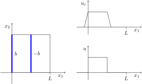
Figure 1: Sketch of the simple situation with two dislocations with Burgers vector $b$ and $-b$ along $\mathbb{R}e_{2}$ and $\mathbb{R}e_{2}+L/2e_{1}$. The right panel illustrates the corresponding values of $u$ and $u_{\varepsilon}$, as defined in (2.10) and (2.11). In all cases, only one period is shown.

In order to understand the appropriate energy scaling, we start from a simple one-dimensional situation. Assume that a dislocation with Burgers vector $b$ is given, along the line $\mathbb{R}e_{2}$ (which is the $x_{2}$ axis), and one with Burgers vector $-b$ along the parallel line $\mathbb{R}e_{2}+L/2e_{1}$, see Figure 1. The sharp-interface model would then have

$$u(x)=\begin{cases}1&\text{ if }kL<x_{1}<(k+\frac{1}{2})L\text{ for some }k\in\mathbb{Z}\,,\\ 0&\text{ otherwise}.\end{cases}$$ (2.10)

It is easy to see that the energy of this slip is infinite, as the elastic energy diverges. A natural regularization on the scale ${\varepsilon}$ is

$$u_{\varepsilon}(x)=\begin{cases}\max\{0,1-\frac{1}{{\varepsilon}}{\mathrm{dist}}(x_{1},[0,L/2])\}&\text{ for }0\leq x_{1}<L\\ \text{periodic extension }&\text{ otherwise.}\end{cases}$$ (2.11)

One can then easily compute that $E_{\varepsilon}[u_{\varepsilon}]\sim\ln 1/{\varepsilon}$. This corresponds to the well-known logarithmic divergence of the energy per unit length of dislocations.

We consider now a situation in which $M$ such dislocations are present. The total energy will be of order $M\ln\frac{1}{{\varepsilon}}$, the total variation of $u_{\varepsilon}$ will be of order $M$, since it has $M$ “jumps” of height 1. Correspondingly, the elastic energy behaves as $M^{2}$. Therefore if $M\sim\ln\frac{1}{{\varepsilon}}$ the total line-tension energy and the total elastic energy are of the same order, see [37, 38, 39] for mathematically rigorous treatments of this heuristics.

For this reason, in the following we shall focus on a situation in which $E_{\varepsilon}[u_{\varepsilon}]$ is of order $(\ln\frac{1}{{\varepsilon}})^{2}$, and $u_{\varepsilon}$ is itself of order $\ln\frac{1}{{\varepsilon}}$. Specifically, we are interested in the limit ${\varepsilon}\to 0$, assuming that

$$\frac{u_{\varepsilon}}{\ln\frac{1}{{\varepsilon}}}\to u_{0}$$ (2.12)

and computing the asymptotic energy (in the sense of $\Gamma$-convergence, see below)

$$\frac{E_{\varepsilon}[u_{\varepsilon}]}{(\ln\frac{1}{{\varepsilon}})^{2}}\to E_{0}[u_{0}]\,.$$ (2.13)

The limiting energy $E_{0}$ will turn out to contain both a long-range elastic energy term and a short-range self-energy term, which characterizes the planar distribution of dislocations. The limiting procedure should be understood as determining the effective energy $E_{0}$ of a limiting plastic slip distribution $u_{0}$ by approximating it with an optimal sequence $u_{\varepsilon}$, and the associated distribution of dislocations, and computing the optimal energy along the sequence.

3 Dislocation line-tension energy

The starting point of our analysis is the line-tension energy approximation derived in [11, 12]. We now briefly review some results which will be needed in the following.

The prelogarithmic factor $\psi_{0}(b,n)$ of a dislocation with Burgers vector $b\in\mathbb{Z}^{N}$ (in the coordinates given in (2.3) above) can be computed as

$$\psi_{0}(b,n)=2\int_{\mathbb{R}}\Gamma(n+tn^{\perp})b\cdot b\,dt$$ (3.1)

where $n^{\perp}=(-n_{2},n_{1})$ is the orthogonal vector to $n$. The vector $n$, in turn, is a unit vector normal to the dislocation line, so that $n^{\perp}$ is the tangential vector. For an elastically isotropic crystal with cubic symmetry, one obtains

$$\psi_{0}^{\mathrm{cubic}}(b,n)=\frac{\mu}{4\pi}\left(|b|^{2}+\eta(b\cdot n)^{2}\right)\,,$$ (3.2)

where $\eta=\nu/(1-\nu)$ is a material parameter which depends on the material’s Poisson’s ratio $\nu$ (see [2, Eq. (51)] or [14, Eq. (4.2)], the latter is missing a factor $1/2$; in [11, 12] a term $\mu/2$ was factored out). The parameter $\eta$ characterizes the relative energy difference between a screw dislocation, which has $b$ orthogonal to $n$, and an edge dislocation, which has $b$ parallel to $n$. The expression (3.2) agrees with the classical energy per unit length of dislocations, as given for example in [4, Eq. (3.13) and (3.52)].

By prelogarithmic factor we mean that the energy per unit length of the dislocation is, to leading order, $\ln\frac{1}{{\varepsilon}}\,\psi_{0}(b,n)$. In the simple case $b=e_{1}$ and $n=e_{1}$, the slip field defined in (2.11) has indeed to leading order energy $\ln\frac{1}{{\varepsilon}}\,\psi_{0}(e_{1},e_{1})$. The reduction of the integration from two to one dimension is made using (2.6), see [9, 12] for details. The prelogarithmic factor $\psi_{0}$ can also be computed directly starting from three-dimensional elasticity, using for example a core-radius regularization. The explicit computation can be done with a suitable plane strain ansatz [4]; a variational characterization minimizing the energy in long cylinders can be found in [17]. All these methods give the same result for $\psi_{0}$, which only depends on the matrix of elastic constants $\mathbb{C}$.

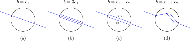
Figure 2: Sketch of some possible microstructures arising in the definition of $\psi_{\mathrm{rel}}$ (3.5). These microstructure arise at the intermediate scale between the one of the lattice and the macroscopic one, as in Figure 3(b).

The prelogarithmic factor $\psi_{0}$ gives, after rescaling, an effective energy per unit length. One can therefore define a line-tension model for a dislocation network. A dislocation network can be parametrized by finitely many oriented curves $\gamma_{1},\dots,\gamma_{M}\subset\mathbb{T}$, each with an associated Burgers vector $b_{1},\dots,b_{M}$, which is a conserved quantity in the sense that for every point $x$, where one or more curves start or end, the sum of the Burgers vectors of the curves ending at $x$ equals the sum of the Burgers vectors of the curves starting at $x$. The (unrelaxed) line-tension energy is then

$$I_{0}=\sum_{i=1}^{M}\int_{\gamma_{i}}\psi_{0}(b_{i},n)ds$$ (3.3)

where $ds$ denotes integration along the curve and $n$ is the normal vector to the curve.

The energy density $\psi_{0}(b,n)$ is quadratic in $b$, as is apparent from the expression in (3.1). This does not, however, reflect the true macroscopic energetic cost of a singularity with total Burgers vector $b$. Consider for example the case that the curve $\gamma_{1}$ has total Burgers vector $b_{1}=(3,0)$. The energy of this is 9 times the energy of a dislocation with the same path and Burgers vector $(1,0)$, since $\psi_{0}(3e_{1},n)=9\psi_{0}(e_{1},n)$. It is therefore energetically convenient to split $\gamma_{1}$ into three dislocations with smaller Burgers vectors, say $\gamma_{1}^{\prime}$, $\gamma_{1}^{\prime\prime}$, $\gamma_{1}^{\prime\prime\prime}$, with $b_{1}^{\prime}=b_{1}^{\prime\prime}=b_{1}^{\prime\prime\prime}=(1,0)$. The three curves have the same start and endpoint as $\gamma_{1}$, but are otherwise disjoint, although very close to each other, and have, up to higher order terms, the same length as $\gamma_{1}$. The total energy along these three curves is then only three times the energy of the original curve (see Figure 2b) This mathematical observation corresponds to the physically well-known fact that only the shortest lattice vectors are stable Burgers vectors of dislocations. In general, this shows that an effective dislocation energy can be stable with respect to decay into parallel dislocations only if it is subattidive in the first argument, a condition which corresponds to the classical Frank’s rule for dislocation reactions [4, 5]. It is important to notice that when we deal with the line tension energy we are considering dislocations at a scale much larger than the lattice spacing, where the core region is identified with a line. Therefore a configuration with a larger total Burgers vector, as the one considered in this examples, that might look unphysical, needs to be understood as a cluster of parallel dislocation lines with short Burgers vectors. The energy $\psi_{0}(3e_{1},n)$ describes the (hypothetical) situation in which the individual lines have a separation of the order of the lattice spacing, so that the total elastic energy of the three dislocations is $9\psi_{0}(e_{1},n)$. The energy $3\psi_{0}(e_{1},n)$ can be achieved if the three dislocations are so close that they can still be identified at a macroscopic scale, but their relative distance is large enough to avoid interaction at the leading order, resulting on an elastic distortion which is the superposition of the effect due to each single dislocation. If the energy computation were attempted numerically, it would be important that the resolution is high enough to resolve the separation of the curves, i.e., the microstructure. In doing the relaxation step analytically, the infinite-resolution limit is automatically incorporated. See Figure 3 for an illustration of the different scales.

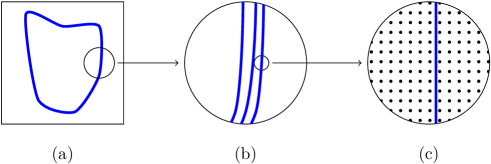
Figure 3: Multiscale relaxation of the dislocation energy. (a) shows a macroscopic dislocation line, whose energy per unit length is characterized by $\psi_{\mathrm{rel}}$. (b) illustrates a blow-up of a small portion of that dislocation, which - in this example - is subdivided into three separate dislocation lines. These lines are very close on the scale of the sample, so that they are not distinguished in (a), but well separated on the scale of the lattice, so that the total energy is the sum $\psi_{0}(b_{1},n)+\psi_{0}(b_{2},n)+\psi_{0}(b_{3},n)$. (c) illustrates a further blow-up, on the scale of the lattice, where only one of the three dislocation lines from (b) is seen.

A less evident instance of the same effect arises for linear combinations of different Burgers vectors. For example, a curve with $b_{1}=(1,1)$ can be replaced by a curve with $b_{1}^{\prime}=(1,0)$ and another one with $b_{1}^{\prime\prime}=(0,1)$, see Figure 2c. Even more, a straight curve may be replaced by a finely-oscillating curve, which has more length but possibly an energetically more convenient orientation (like in faceting of crystal surfaces), see Figure 2d. Whether this is energetically convenient depends on the details of the problem, including in particular the orientation of the dislocation line and the material’s elastic constants. For a more detailed discussion of these phenomena we refer to [11, 17], and to [40, 41, 14] for the mathematical background.

The optimal energy per unit length of a dislocation network that carries the total Burgers vector $b\in\mathbb{Z}^{N}$ across a segment with normal $n\in S^{1}$ is given by the cell-problem formula

$$\psi_{\mathrm{rel}}(b,n)=\inf\Bigl{\{}\sum_{i}\int_{\gamma_{i}}\psi_{0}(b_{i},\nu)ds\Bigr{\}}$$ (3.4)

where the minimum is taken over all networks as described above, which start in the point 0 with a Burgers vector $b$, and end in the point $n^{\perp}$ with the same Burgers vector, $\nu$ is the normal to the dislocation line $\gamma_{i}$. This minimization corresponds to the optimization among all possible dislocation structures which are admissible, in the sense that the total Burgers vector is conserved, and which agree with a straight dislocation with total Burgers vector $b$ and normal $n$ outside a small region, as illustrated in Figure 2.

An equivalent formulation can be given in terms of piecewise constant phase fields, which correspond to functions of bounded variation with values in $\mathbb{Z}^{N}$. Indeed,

$$\psi_{\mathrm{rel}}(b,n)=\inf\Bigl{\{}\frac{1}{2}\int_{J_{u}}\psi_{0}([u],\nu_{u})d\mathcal{H}^{1}:u\in BV(B_{1},\mathbb{Z}^{N}),\,u=u^{b,n}\text{ on }\partial B_{1}\Bigr{\}}$$ (3.5)

where $u^{b,n}(x)=0$ if $x\cdot n<0$, and $b$ if $x\cdot n>0$, and $B_{1}$ the ball of unit radius centered in the origin, which has diameter $2$. Here $J_{u}$ is the set where $u$ jumps, which corresponds to the union of the dislocation curves $\gamma_{i}$, $[u]$ is the jump, which corresponds to the local Burgers vector, and $\nu_{u}$ the normal to $J_{u}$. For $u^{b,n}$, the jump set is the diameter of $B_{1}$ orthogonal to $n$, the jump equals $b$, and therefore setting $u=u^{b,n}$ in (3.5) yields $\psi_{\mathrm{rel}}(b,n)\leq\psi_{0}(b,n)$. Here and below $\mathcal{H}^{1}$ denotes integration along the (one-dimensional) set $J_{u}$. We refer to [42] for precise definitions of these concepts.

By [17, Lemma 6.4] one can show that

$$\psi_{\mathrm{rel}}(b,n)=\inf\Bigl{\{}\frac{1}{2}\int_{J_{u}}\psi_{0}([u],\nu_{u})d\mathcal{H}^{1}:u\in PC(B_{1},\mathbb{Z}^{N}),\,u=u^{b,n}\text{ on }\partial B_{1}\Bigr{\}}$$ (3.6)

where, given $\omega\subset\mathbb{R}^{2}$ and a set $A$, we denote by $PC(\omega;A)$ the set of polygonal piecewise affine functions with values in $A$, i.e., the set of functions $u:\omega\to A$ such that $\omega$ can be covered by finitely many disjoint polygons, such that $u$ is constant on each of them. In particular, the construction in Figure 2(b) permits to prove that $\psi_{\mathrm{rel}}(b,n)$ has linear growth in $b$, in the sense that

$$\frac{1}{c}|b|\leq\psi_{\mathrm{rel}}(b,n)\leq c|b|\text{ for all }n\in S^{1},b\in\mathbb{Z}^{N}\,.$$ (3.7)

Starting from Michael Ortiz’s phase field model, in [9, 11, 12] it was shown that, in the regime in which the energy is proportional to $\ln\frac{1}{{\varepsilon}}$, the energetically optimal slips correspond to a dislocation distribution with finite total length, whose energy can be computed at leading order using $\psi_{\mathrm{rel}}$. Precisely, this can be expressed in terms of $\Gamma$-convergence as

$$\frac{1}{\ln(1/{\varepsilon})}E_{\varepsilon}\stackrel{{\scriptstyle\Gamma}}{{\to}}E_{0}^{*}$$ (3.8)

where

$$E_{0}^{*}[u]=\int_{J_{u}}\psi_{\mathrm{rel}}([u],n)d\mathcal{H}^{1}\text{ for }u\in BV(\mathbb{T};\mathbb{Z}^{N})\,.$$ (3.9)

The convergence in (3.8) means that for any sequence $u_{\varepsilon}\to u_{0}$ one has

$$E_{0}^{*}[u_{0}]\leq\liminf_{{\varepsilon}\to 0}\frac{1}{\ln(1/{\varepsilon})}E_{\varepsilon}[u_{\varepsilon}]$$ (3.10)

and, conversely, that for any $u_{0}$ there is a sequence $u_{\varepsilon}\to u_{0}$ such that

$$E_{0}^{*}[u_{0}]=\lim_{{\varepsilon}\to 0}\frac{1}{\ln(1/{\varepsilon})}E_{\varepsilon}[u_{\varepsilon}]\,,$$ (3.11)

see [43, 44]. This corresponds to the fact that $E_{0}^{*}[u_{0}]$ is the smallest energy, to leading order, among all sequences $u_{\varepsilon}$ converging to $u_{0}$ in $L^{1}(\mathbb{T};\mathbb{R}^{N})$.

The scaling of the energy in (3.8) and the convergence $u_{\varepsilon}\to u_{0}$ used in [9, 11, 12] are appropriate to emphasize the line-tension energy of individual dislocation lines. In contrast, in the present work we focus on a different regime, characterized by (2.12) and (2.13), which is appropriate for computing the total energy of a complex dislocation structure, consisting of a large number of individual dislocation lines, as will be explained in the next section.

4 Cell structures and their energy

Figure 4: Approximation of a continuous slip by a step process with many individual dislocations.

We now study macroscopically continuous slip. Passing to a larger scale, one sees a large number of dislocations, with a large total Burgers vector, which may be approximately uniformly distributed in space, see Figure 4. This is the same procedure that is usually used to study low-angle grain boundaries or the opening of cracks, see for example [6, 45, 46]. Consider for definiteness a locally affine slip, $v(x)=Ax$, for some matrix $A\in\mathbb{R}^{N\times 2}$. Before presenting the general situation, we start from the illustrative example $A=e_{1}\otimes e_{1}-e_{2}\otimes e_{2}$. We write

$$\hat{u}_{\sigma}(x)=e_{1}\left\lfloor\frac{x_{1}}{\sigma}\right\rfloor-e_{2}\left\lfloor\frac{x_{2}}{\sigma}\right\rfloor\,,$$ (4.1)

where $\sigma$ is a small parameter and $\lfloor y\rfloor=\max\{z\in\mathbb{Z}:z\leq y\}$ denotes the largest integer not larger than $y$. This is a piecewise constant function, which for small $\sigma$ is close to $Ax/\sigma$ and jumps across horizontal and vertical lines spaced by $\sigma$, which represent the dislocations. The amplitudes of the jumps are $e_{2}$ and $e_{1}$, respectively (see Figure 5). The energy per unit area of this configuration can be computed using (3.3) and is $\frac{1}{\sigma}\psi_{0}(e_{1},e_{1})+\frac{1}{\sigma}\psi_{0}(e_{2},e_{2})$. As above, the energy can in principle be reduced by local microstructures, leading to relaxation, the corresponding energy will be obtained using $\psi_{\mathrm{rel}}$ instead of $\psi_{0}$.

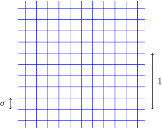
Figure 5: Sketch of possible simple grid structures as defined in (4.1) and (4.2), corresponding to the macroscopic slip $u(x)=Ax=(x_{1},-x_{2})$.

Since both the slip and the energy are diverging as $\sigma$ tends to zero, it is convenient to rescale. We multiply both the slip and the energy by $\sigma$ and obtain the sequence of slip fields

$$u_{\sigma}(x)=e_{1}\sigma\left\lfloor\frac{x_{1}}{\sigma}\right\rfloor-e_{2}\sigma\left\lfloor\frac{x_{2}}{\sigma}\right\rfloor$$ (4.2)

converging to $Ax$ for small $\sigma$. Its jump set has (locally) length diverging as $1/\sigma$, but its jumps have amplitude $\sigma$. It is then natural to correspondingly rescale the energy density, and to consider

$${\psi_{\infty}(b,n)=\liminf_{\sigma\to 0}\sigma\,\psi_{\mathrm{rel}}(\frac{b}{\sigma},n)=\liminf_{s\to\infty}\frac{1}{s}\psi_{\mathrm{rel}}(sb,n)\,.}$$ (4.3)

This limit is finite since $\psi_{\mathrm{rel}}$ has linear growth (recall (3.7)), the new function $\psi_{\infty}$ captures the asymptotic behavior of $\psi_{\mathrm{rel}}$ at infinity, i.e., the approximate energy per unit length and unit Burgers vector.

The map $u_{\sigma}$ jumps, within the unit square $[0,1)^{2}$, on $\lceil 1/\sigma\rceil$ horizontal segments of unit length, and the jump amplitude is $\sigma e_{2}$ (with $\lceil y\rceil=\min\{z\in\mathbb{Z}:z\geq y\}$, since $\psi_{0}^{\mathrm{cubic}}$ is an even function the orientation does not matter). Their (scaled) total energy is $\lceil\frac{1}{\sigma}\rceil\psi_{\infty}(\sigma e_{2},e_{2})$. The same holds for the jumps over horizontal lines, and the energy per unit area of $u_{\sigma}$ is

$$\lceil\frac{1}{\sigma}\rceil\psi_{\infty}(\sigma e_{1},e_{1})+\lceil\frac{1}{\sigma}\rceil\psi_{\infty}(\sigma e_{2},e_{2})\sim\psi_{\mathrm{rel}}(e_{1},e_{1})+\psi_{\mathrm{rel}}(e_{2},e_{2})\,.$$ (4.4)

In many cases, however, more complicated structures appear. Consider for example the pattern illustrated in Figure 6. Here the two sets of dislocations interact, and overlap over part of the domain to form a composite dislocation with a larger Burgers vector parallel to $(1,1)$. In order to compute the energy of this configuration, we assume that the central segment is oriented at $45$ degrees and denote by $2\delta\in[0,\sigma)$ the length of its horizontal projection, see Figure 6(b). The energy of this central segment is $2\delta\sqrt{2}\psi_{\infty}(\sigma(e_{1}+e_{2}),{(e_{1}-e_{2})/\sqrt{2})}$. The lower segment has length $\sqrt{\delta^{2}+(\sigma/2-\delta)^{2}}$, normal $\bar{n}=(\sigma/2-\delta,\delta)/\sqrt{\delta^{2}+(\sigma/2-\delta)^{2}}$, and Burgers vector $\sigma e_{1}$. Therefore its energy is

$$\sqrt{\delta^{2}+(\sigma/2-\delta)^{2}}\psi_{\infty}(\sigma e_{1},\bar{n})\,.$$ (4.5)

Correspondingly, the segment on the left has energy

$$\sqrt{\delta^{2}+(\sigma/2-\delta)^{2}}\psi_{\infty}(\sigma e_{2},\bar{n}^{\prime})$$ (4.6)

where $\bar{n}^{\prime}=(\delta,\sigma/2-\delta)/\sqrt{\delta^{2}+(\sigma/2-\delta)^{2}}$. The other two are the same, up a translation. The energy in the $(0,\sigma)^{2}$ square is therefore

$$e(\delta)= 2\delta\sqrt{2}{\psi_{\infty}(\sigma(e_{1}+e_{2}),(e_{1}-e_{2})/\sqrt{2})}$$

$$+2\sqrt{\delta^{2}+(\sigma/2-\delta)^{2}}\left(\psi_{\infty}(\sigma e_{1},\bar{n})+\psi_{\infty}(\sigma e_{2},\bar{n}^{\prime})\right)\,.$$ (4.7)

We now show that, at least in the case of a cubic crystal with isotropic elasticity, this configuration is energetically more convenient than the simple one described in (4.2) and Figure 5 above, and which corresponds to the $\delta=0$ case of the present one. For cubic crystals we know that $\psi_{0}$ is given by (3.2). Further, it was shown in [14, Lemma 4.4] that

$$\psi_{\mathrm{rel}}^{\mathrm{cubic}}(ke_{i},n)={|k|}\psi^{\mathrm{cubic}}_{0}(e_{i},n)\text{ for $i=1,2$, $k\in\mathbb{Z}$ and $n\in S^{1}$. }$$ (4.8)

From [14, Lemma 4.6] using $\psi^{\mathrm{cubic}}_{0}(e_{1}+e_{2},(e_{1}-e_{2})/\sqrt{2})=2\leq\psi^{\mathrm{cubic}}_{0}(e_{1}+e_{2},n)$ one easily sees that

$$\psi_{\mathrm{rel}}^{\mathrm{cubic}}(k(e_{1}+e_{2}),\frac{e_{1}-e_{2}}{\sqrt{2}})={|k|}\psi^{\mathrm{cubic}}_{0}((e_{1}+e_{2}),\frac{e_{1}-e_{2}}{\sqrt{2}})\text{ for $k\in\mathbb{Z}$ }\,.$$ (4.9)

In particular, recalling (3.2) and (4.3), we obtain

$$\psi_{\infty}^{\mathrm{cubic}}(ke_{i},n)=\frac{\mu}{4\pi}|k|(1+\eta(n\cdot e_{i})^{2})$$ (4.10)

and

$$\psi_{\infty}^{\mathrm{cubic}}(k(e_{1}+e_{2}),\frac{e_{1}-e_{2}}{\sqrt{2}})=\frac{\mu}{4\pi}2|k|\,.$$ (4.11)

Inserting in (4.7) we obtain

$$e(\delta) =4\sigma\frac{\mu}{4\pi}\left[\sqrt{\delta^{2}+(\frac{1}{2}\sigma-\delta)^{2}}+\eta\frac{(\frac{1}{2}\sigma-\delta)^{2}}{\sqrt{\delta^{2}+(\frac{1}{2}\sigma-\delta)^{2}}}+\delta\sqrt{2}\right]$$ (4.12)

$$=4\sigma^{2}\frac{\mu}{4\pi}\left[\frac{1+\eta}{2}+\frac{\delta}{\sigma}(\sqrt{2}-1-\eta)+O\left(\frac{\delta^{2}}{\sigma^{2}}\right)\right]\,.$$ (4.13)

Therefore for $\eta>\sqrt{2}-1$ the minimum of $e$ is not taken at $\delta=0$. For example, if $\eta=1/2$ the optimal value is taken at $\delta\sim 0.07\sigma$, leading to the pattern illustrated in Figure 6. Recalling that $\eta=\nu/(1-\nu)$, we can easily see that the condition $\eta>\sqrt{2}-1$ corresponds to

$$\nu>1-\frac{1}{\sqrt{2}}\sim 0.29\,,$$ (4.14)

which is satisfied in many metals. The specific value $\eta=1/2$ chosen for the computation above corresponds to $\nu=1/3$. We remark that this result, although mathematically rigorous under the stated assumptions, depends on the chosen orientation and the chosen elastic properties. Further, its physical relevance is restricted by the assumptions of the current modeling, which in particular focuses on the leading-order energy terms with respect to the small parameter ${\varepsilon}$.

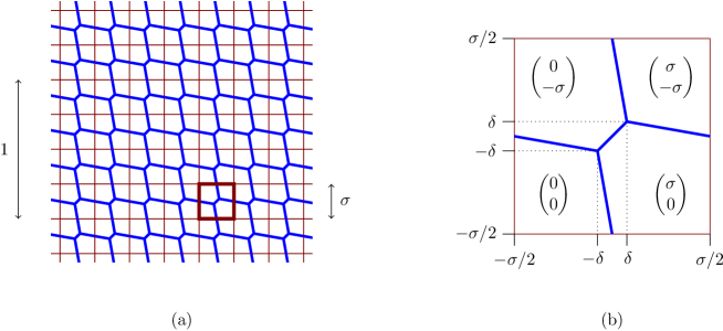
Figure 6: Sketch of a more complex microstructure with the energy given in (4.7). (a) shows a larger region, (b) a blow-up of a $\sigma\times\sigma$ square on which the computation is performed. For $\delta=0$ this reduces to the microstructure in Figure 5.

As illustrated in the above examples, we define the energy per unit area of a general affine slip field $u(x)=Ax$ by considering the optimal energy of dislocation networks which realize it. We start from the rescaled energy density defined in (4.3). We define $g:\mathbb{R}^{M\times 2}\to[0,\infty)$ by the cell problem

$$g(A)=\inf\Bigl{\{}\liminf_{j\to\infty}\frac{1}{\pi}\int_{J_{u_{j}}\cap B_{1}}\psi_{\infty}([u_{j}],{\nu_{u_{j}}})\,d\mathcal{H}^{1}:\ u_{j}\text{ piecewise constant,}$$ (4.15)

$$u_{j}(x)\to Ax\text{ in }L^{1}(B_{1})\Bigr{\}}$$

where the set of piecewise constant functions $PC(B_{1},\mathbb{R}^{N})$ was defined after (3.6). We remark that periodicity does not play a role here, as $g$ will be used for the local energy in a representative volume element, where the macroscopic slip field is approximately affine with gradient $A$. The minimization in (4.15) is by itself a complex problem, which in general can only be attacked numerically. The study of efficient tools for this procedure and of possible explicit solutions in special cases constitutes an interesting direction of further work.

It is important to notice that the function $g$ is quasiconvex, continuous, one homogeneous, and has linear growth, in the sense that $\frac{1}{c}|A|\leq g(A)\leq c|A|$ for all matrices $A$. A detailed proof of those facts will appear elsewhere [47].

We now pass from the local picture to a macroscopic slip field. Let $u:\mathbb{T}\to\mathbb{R}^{N}$ be a slip field, which for now we assume to be continuously differentiable. Around every point $x\in\mathbb{T}$, the local energy of the dislocations corresponding to $\nabla u$ is determined by the energy $g(\nabla u)$ of the optimal network realizing this gradient, as defined in (4.15). We therefore obtain the expression

$$E_{\mathrm{netw}}[u]=\int_{\mathbb{T}}g(\nabla u)dx\,,$$ (4.16)

valid for $u\in C^{1}(\mathbb{T};\mathbb{R}^{N})$. If the slip field is not smooth, an additional approximation procedure is needed. This leads to the expression

$$E_{\mathrm{\mathrm{self}}}[u]=\int_{\mathbb{T}}g(\nabla u)dx+\int_{\mathbb{T}}g(\frac{dD^{s}u}{d|D^{s}u|})d|D^{s}u|$$ (4.17)

for $u\in BV(\mathbb{T};\mathbb{R}^{N})$. Here $D^{s}u$ is the singular part of the distributional gradient of $u$, which may contain both jump parts and diffuse parts, and $\nabla u$ is the absolutely continuous part. Inded, for any $u\in BV(\mathbb{T};\mathbb{R}^{N})$ one writes $Du=\nabla u\mathcal{L}^{2}+D^{s}u$, where $\nabla u\in L^{1}(\mathbb{T};\mathbb{R}^{N\times 2})$ and $D^{s}u$ is a measure on $\mathbb{T}$ with values in $\mathbb{R}^{N\times 2}$, concentrated on a set of Lebesgue measure equal to zero. Typical instances of singular measures are a Dirac measure concentrated on a segment, corresponding to the derivative of a discontinuous function, and a measure concentrated on a fractal, such as the Cantor set. For example, for a given matrix $A_{*}\in\mathbb{R}^{N\times 2}$, the slip

$$u_{*}(x)=\begin{cases}A_{*}x&\text{ if }0<x_{1}<L/2\\ 0&\text{ otherwise}\end{cases}$$ (4.18)

would have a continuous dislocation density $A_{*}$ for $0<x_{1}<L/2$, and a concentrated dislocation density along the $\{x_{1}=0\}$ and $\{x_{1}=L/2\}$ lines. The jump in $u_{*}$ at the point $(0,t)$ equals $u_{*}(0^{+},t)-u_{*}(0^{-},t)=A_{*}e_{2}t$; the distributional gradient is oriented along the normal to the singularity, which is $e_{1}$. The same holds for $x_{1}=L/2$. Inserting in the above expression we obtain that the self-energy associated with $u_{*}$ reads

$$E_{\mathrm{\mathrm{self}}}[u_{*}]=\int_{\{0<x_{1}<L/2\}}g(A_{*})dx+2\int_{0}^{L}g(tA_{*}e_{2}\otimes e_{1})dt\,.$$ (4.19)

We refer to [42] for further details. The fact that $E_{\mathrm{\mathrm{self}}}$ is the relaxation of $E_{\mathrm{netw}}$ follows, for example, from the general results on relaxation of $BV$ functionals in [48] or [49]. In particular, this implies that $E_{\mathrm{\mathrm{self}}}$ is lower semicontinuous.

5 The effective limiting energy

The limiting process discussed above, with subsequent rescalings, can be directly obtained starting from the phase-field model in a suitable scaling regime which permits the total length of the dislocation lines to diverge as ${\varepsilon}\to 0$. As discussed above, we focus on the regime in which the elastic displacement scales as $\ln\frac{1}{{\varepsilon}}$, so that the relevant convergence of displacements is (see discussion around (2.12))

$$\frac{u_{\varepsilon}}{\ln\frac{1}{{\varepsilon}}}\to u_{0}\,.$$ (5.1)

Correspondingly, the energy $E_{\varepsilon}$ is assumed to be proportional to $(\ln\frac{1}{{\varepsilon}})^{2}$. We will determine the limit (in the sense of $\Gamma$-convergence) of the quotients

$$\frac{1}{(\ln\frac{1}{{\varepsilon}})^{2}}E_{\varepsilon}\stackrel{{\scriptstyle\Gamma}}{{\to}}E_{0}$$ (5.2)

as in (2.13). This scaling was chosen so that the self-interaction leading to line-tension effects balances the macroscopic elastic energy.

The limiting functional is given by the sum of the self-energy and the elastic energy,

$$E_{0}[u]=E_{\mathrm{\mathrm{self}}}[u]+\int_{\mathbb{T}\times\mathbb{T}}K(z)(u(x)-u(x+z))\cdot(u(x)-u(x+z))\,dx\,dz\,,$$ (5.3)

with $E_{\mathrm{\mathrm{self}}}$ defined in (4.17). The proof, which is mathematically very technical and builds upon $BV$ relaxation techniques from [48] and [49] and the lower bound for the case of finite dislocation length in [12], will be presented elsewhere [47]. One key idea is that the self-energy $E_{\mathrm{\mathrm{self}}}$ arises from the short-range part of the interaction. Precisely, one can show that, for any $\rho>0$,

$$\begin{split}\frac{1}{(\ln\frac{1}{{\varepsilon}})^{2}}\int_{\mathbb{T}}\left(\int_{B_{\rho}(0)}K(z)(u_{\varepsilon}(x)-u_{\varepsilon}(x+z))\cdot(u_{\varepsilon}(x)-u_{\varepsilon}(x+z))dz\right)dx\\ \to E_{\mathrm{\mathrm{self}}}[u]\,,\end{split}$$ (5.4)

for an optimal sequence $u_{\varepsilon}$ converging to $u$ as in (5.1). The fact that the limit does not depend on $\rho$ corresponds to the fact that the line-tension energy $\psi_{0}$, which then originates $\psi_{\mathrm{rel}}$, $\psi_{\infty}$ and $g$, is localized on a small neighbourhood of the dislocation, whose size is, as ${\varepsilon}\to 0$, much larger than ${\varepsilon}$, but smaller than the (fixed) length $\rho$.

At the same time, the part of the energy with $|z|>\rho$ is continuous in the limit, and

$$\frac{1}{(\ln\frac{1}{{\varepsilon}})^{2}}\int_{\mathbb{T}}\left(\int_{\mathbb{T}\setminus B_{\rho}(0)}K(z)(u_{\varepsilon}(x)-u_{\varepsilon}(x+z))\cdot(u_{\varepsilon}(x)-u_{\varepsilon}(x+z))dz\right)dx$$

$$\to\int_{\mathbb{T}}\left(\int_{\mathbb{T}\setminus B_{\rho}(0)}K(z)(u(x)-u(x+z))\cdot(u(x)-u(x+z))dz\right)dx\,.$$ (5.5)

The proof is based on making these two assertions rigorous, showing that the optimal sequence can be chosen to be the same for both, and taking the limit $\rho\to 0$.

We finally transfer our result back into the 3D setting discussed in the introduction. Let $U:\mathbb{T}\times\mathbb{R}\to\mathbb{R}^{3}$ be a deformation, with slip field $\gamma=[U]$. The self-energy of the slip field is then obtained using the change of variables performed in (2.3) to express the slip field in a basis of Burgers vectors. Precisely, one obtains

$$F_{\mathrm{\mathrm{self}}}[\gamma]=\int_{\mathbb{T}}f(\nabla\gamma)dx+\int_{\mathbb{T}}f(\frac{dD^{s}\gamma}{d|D^{s}\gamma|})d|D^{s}\gamma|$$ (5.6)

for $\gamma\in BV(\mathbb{T};\mathbb{R}^{2}\times\{0\})$, where $f$ is defined by the change of variables $f(\sum_{i=1}^{N}s_{i}\otimes c_{i})=g(\sum_{i=1}^{N}e_{i}\otimes c_{i})$ for any $c_{i}\in\mathbb{R}^{2}$ (here $\{s_{i}\}$ denotes the basis of $\mathcal{B}$ chosen in (2.3) and $\{e_{i}\}$ the canonical basis of $\mathbb{R}^{N}$). Therefore the functional

$$\frac{1}{(\ln(1/{\varepsilon})^{2}}\left[\frac{1}{{\varepsilon}}\int_{\mathbb{T}}W_{\mathcal{B}}(\gamma_{\varepsilon})dx+\int_{\mathbb{T}\times\mathbb{R}}\frac{1}{2}\mathbb{C}e(U_{\varepsilon})\cdot e(U_{\varepsilon})\,dx\right]$$ (5.7)

(with $\gamma_{\varepsilon}=[U_{\varepsilon}]$) $\Gamma$-converges, as ${\varepsilon}\to 0$, to the functional

$$F_{0}[U]=\int_{\mathbb{T}}f(\nabla\gamma)dx+\int_{\mathbb{T}}f(\frac{dD^{s}\gamma}{d|D^{s}\gamma|})d|D^{s}\gamma|+\int_{\mathbb{T}\times\mathbb{R}}\frac{1}{2}\mathbb{C}e(U)\cdot e(U)\,dx$$ (5.8)

where $\gamma=[U]$. The relevant convergence of the displacement fields is $U_{\varepsilon}/\ln(1/{\varepsilon})\to U$, which implies $\gamma_{\varepsilon}/\ln(1/{\varepsilon})\to\gamma$ for the corresponding slip fields. We remark that, expressed in the physical dislocation density tensor $\alpha\sim u_{0}\ln\frac{1}{{\varepsilon}}$, the self-energy of the networks scales as $(\ln\frac{1}{{\varepsilon}})^{2}F_{0}[u_{0}]\sim\ln\frac{1}{{\varepsilon}}\alpha$.

6 Conclusions and outlook

We have discussed a new facet of the phase-field model developed by Michael Ortiz and coworkers in the 90s, and shown that it permits a rigorous analytical study of dislocation networks in the plane, which accounts for the self-energy of the dislocations and the long-range elastic energy. We discussed how the effective energy for dislocation microstructures can be computed by solving an appropriate cell problem in each representative volume element. The analysis of the cell problem itself leads to the prediction, under specific circumstances, of complex dislocation networks in the plane, with interaction between dislocations in different directions, as illustrated in Figure 6. Our derivation of the functional $F_{0}$ supports the use of strain-gradient models in plasticity with linear growth of the strain gradient term, as was done for example in [26, 33]. At the same time the current derivation adds more details to these models, as the self-energy is rigorously derived from the material properties. In particular, the cell structure illustrated in Figure 6 is a direct consequence of the specific form of the self-energy in cubic crystals, and would not appear with the simpler self-energy used in [26]. Although the framework we formulated is completely general, our specific analysis is restricted to a cubic geometry. It would be interesting to extend the analysis to the commonly seen dislocation structures, as for example to the geometry appropriate for $111$ planes of fcc crystals, which have a triangular structure.

References

References

- Ortiz [1999] M. Ortiz, Plastic yielding as a phase transition, J. Appl. Mech.-Trans. ASME 66 (1999) 289–298.
- Koslowski et al. [2002] M. Koslowski, A. M. Cuitiño, M. Ortiz, A phase-field theory of dislocation dynamics, strain hardening and hysteresis in ductile single crystal, J. Mech. Phys. Solids 50 (2002) 2597–2635.
- Koslowski and Ortiz [2004] M. Koslowski, M. Ortiz, A multi-phase field model of planar dislocation networks, Model. Simul. Mat. Sci. Eng. 12 (2004) 1087–1097.
- Hirth and Lothe [1968] J. P. Hirth, J. Lothe, Theory of Dislocations, McGraw-Hill, New York, 1968.
- Hull and Bacon [2011] D. Hull, D. J. Bacon, Introduction to dislocations, 5th ed., Butterworth-Heinemann, Oxford, UK, 2011.
- Xu and Ortiz [1993] G. Xu, M. Ortiz, A variational boundary integral method for the analysis of 3-D cracks of arbitrary geometry modelled as continuous distributions of dislocation loops, International journal for numerical methods in engineering 36 (1993) 3675–3701.
- Xu and Argon [2000] G. Xu, A. S. Argon, Homogeneous nucleation of dislocation loops under stress in perfect crystals, Philosophical magazine letters 80 (2000) 605–611.
- Xiang et al. [2008] Y. Xiang, H. Wei, P. Ming, E. Weinan, A generalized Peierls–Nabarro model for curved dislocations and core structures of dislocation loops in Al and Cu, Acta materialia 56 (2008) 1447–1460.
- Garroni and Müller [2005] A. Garroni, S. Müller, -limit of a phase-field model of dislocations, SIAM J. Math. Anal. 36 (2005) 1943–1964.
- Garroni and Müller [2006] A. Garroni, S. Müller, A variational model for dislocations in the line tension limit, Arch. Ration. Mech. Anal. 181 (2006) 535–578.
- Cacace and Garroni [2009] S. Cacace, A. Garroni, A multi-phase transition model for the dislocations with interfacial microstructure, Interfaces Free Bound. 11 (2009) 291–316.
- Conti et al. [2011] S. Conti, A. Garroni, S. Müller, Singular kernels, multiscale decomposition of microstructure, and dislocation models, Arch. Rat. Mech. Anal. 199 (2011) 779–819.
- Conti and Gladbach [2015] S. Conti, P. Gladbach, A line-tension model of dislocation networks on several slip planes, Mechanics of Materials 90 (2015) 140–147.
- Conti et al. [2015] S. Conti, A. Garroni, A. Massaccesi, Modeling of dislocations and relaxation of functionals on 1-currents with discrete multiplicity, Calc. Var. PDE 54 (2015) 1847–1874.
- Ariza and Ortiz [2005] M. P. Ariza, M. Ortiz, Discrete crystal plasticity, Arch. Ration. Mech. Anal. 178 (2005) 149–226.
- Ramasubramaniam et al. [2007] A. Ramasubramaniam, M. P. Ariza, M. Ortiz, A discrete mechanics approach to dislocation dynamics in bcc crystals, J. Mech. Phys. Solids 55 (2007) 615–647.
- Conti et al. [2015a] S. Conti, A. Garroni, M. Ortiz, The line-tension approximation as the dilute limit of linear-elastic dislocations, Arch. Ration. Mech. Anal. 218 (2015a) 699–755.
- Conti et al. [2015b] S. Conti, A. Garroni, M. Ortiz, From atomic interactions to the line-tension approximation for dilute dislocations, in preparation (2015b).
- Barnett and Swanger [1971] D. Barnett, L. Swanger, The elastic energy of a straight dislocation in an infinite anisotropic elastic medium, Physica Status Solidi 48 (1971) 419–428.
- Rice [1985] J. R. Rice, Conserved integrals and energetic forces, in: K. J. Miller (Ed.), Fundamentals of Deformation and Fracture, Cambridge University Press, 1985.
- Gottstein [2014] G. Gottstein, Materialwissenschaft und Werkstofftechnik: Physikalische Grundlagen, Springer-Verlag, 2014.
- Fleck and Hutchinson [1993] N. A. Fleck, J. W. Hutchinson, A phenomenological theory for strain gradient effects in plasticity, J. Mech. Phys. Solids 41 (1993) 1825–1857.
- Nix and Gao [1998] W. D. Nix, H. J. Gao, Indentation size effects in crystalline materials: A law for strain gradient plasticity, J. Mech. Phys. Solids 46 (1998) 411–425.
- Fleck and Hutchinson [2001] N. A. Fleck, J. W. Hutchinson, A reformulation of strain gradient plasticity, J. Mech. Phys. Solids 49 (2001) 2245–2271.
- Bassani [2001] J. L. Bassani, Incompatibility and a simple gradient theory of plasticity, J. Mech. Phys. Solids 49 (2001) 1983–1996.
- Conti and Ortiz [2005] S. Conti, M. Ortiz, Dislocation microstructures and the effective behavior of single crystals, Arch. Rat. Mech. Anal. 176 (2005) 103–147.
- Kuroda and Tvergaard [2008] M. Kuroda, V. Tvergaard, On the formulations of higher-order strain gradient crystal plasticity models, J. Mech. Phys. Solids 56 (2008) 1591–1608.
- Fokoua et al. [2014] L. Fokoua, S. Conti, M. Ortiz, Optimal scaling laws for ductile fracture derived from strain-gradient microplasticity, J. Mech. Phys. Solids 62 (2014) 295–311.
- Aubry and Ortiz [2003] S. Aubry, M. Ortiz, The mechanics of deformation-induced subgrain-dislocation structures in metallic crystals at large strains, Proc. R. Soc. Lond. A 459 (2003) 3131–3158.
- Ortiz and Repetto [1999] M. Ortiz, E. Repetto, Nonconvex energy minimization and dislocation structures in ductile single crystals, J. Mech. Phys. Solids 47 (1999) 397–462.
- Conti and Theil [2005] S. Conti, F. Theil, Single-slip elastoplastic microstructures, Arch. Rat. Mech. Anal. 178 (2005) 125–148.
- Conti et al. [2013] S. Conti, G. Dolzmann, C. Kreisbeck, Relaxation of a model in finite plasticity with two slip systems, Math. Models Methods Appl. Sci. 23 (2013) 2111–2128.
- Anguige and Dondl [2014] K. Anguige, P. Dondl, Relaxation of the single-slip condition in strain-gradient plasticity, R. Soc. Lond. Proc. Ser. A Math. Phys. Eng. Sci. 470 (2014).
- Hunter and Koslowski [2008] A. Hunter, M. Koslowski, Direct calculations of material parameters for gradient plasticity, Journal of the Mechanics and Physics of Solids 56 (2008) 3181–3190.
- Xiang [2009] Y. Xiang, Continuum approximation of the peach–koehler force on dislocations in a slip plane, Journal of the Mechanics and Physics of Solids 57 (2009) 728–743.
- Zhu and Xiang [2014] X. Zhu, Y. Xiang, Continuum framework for dislocation structure, energy and dynamics of dislocation arrays and low angle grain boundaries, Journal of the Mechanics and Physics of Solids 69 (2014) 175–194.
- Garroni et al. [2010] A. Garroni, G. Leoni, M. Ponsiglione, Gradient theory for plasticity via homogenization of discrete dislocations, J. Eur. Math. Soc. (JEMS) 12 (2010) 1231–1266.
- Müller et al. [2014] S. Müller, L. Scardia, C. I. Zeppieri, Geometric rigidity for incompatible fields and an application to strain-gradient plasticity, Indiana Univ. Math. J. 63 (2014) 1365–1396.
- Müller et al. [2015] S. Müller, L. Scardia, C. I. Zeppieri, Gradient theory for geometrically nonlinear plasticity via the homogenization of dislocations, in: S. Conti, K. Hackl (Eds.), Analysis and Computation of Microstructure in Finite Plasticity, Springer, 2015, pp. 175–204.
- Ambrosio and Braides [1990a] L. Ambrosio, A. Braides, Functionals defined on partitions in sets of finite perimeter. I. Integral representation and -convergence, J. Math. Pures Appl. (9) 69 (1990a) 285–305.
- Ambrosio and Braides [1990b] L. Ambrosio, A. Braides, Functionals defined on partitions in sets of finite perimeter. II. Semicontinuity, relaxation and homogenization, J. Math. Pures Appl. (9) 69 (1990b) 307–333.
- Ambrosio et al. [2000] L. Ambrosio, N. Fusco, D. Pallara, Functions of Bounded Variation and Free Discontinuity Problems, Mathematical Monographs, Oxford University Press, 2000.
- Dal Maso [1993] G. Dal Maso, An introduction to -convergence, Progress in Nonlinear Differential Equations and their Applications, 8, Birkhäuser Boston Inc., Boston, MA, 1993.
- Braides [2002] A. Braides, Gamma-convergence for Beginners, Oxford University Press, 2002.
- Bulatov and Kaxiras [1997] V. V. Bulatov, E. Kaxiras, Semidiscrete variational peierls framework for dislocation core properties, Physical review letters 78 (1997) 4221.
- Dai et al. [2013] S. Dai, Y. Xiang, D. J. Srolovitz, Structure and energy of (111) low-angle twist boundaries in Al, Cu and Ni, Acta materialia 61 (2013) 1327–1337.
- Conti et al. [2015] S. Conti, A. Garroni, S. Müller, Derivation of the dislocation self-energy from a planar phase-field model, in preparation (2015).
- Ambrosio and Dal Maso [1992] L. Ambrosio, G. Dal Maso, On the relaxation in of quasi-convex integrals, J. Funct. Anal. 109 (1992) 76–97.
- Fonseca and Müller [1993] I. Fonseca, S. Müller, Relaxation of quasiconvex functionals in for integrands , Arch. Rational Mech. Anal. 123 (1993) 1–49.