Hot Jupiter Breezes:
Time-dependent Outflows from Extrasolar Planets

Abstract

We explore the dynamics of magnetically controlled outflows from Hot Jupiters, where these flows are driven by UV heating from the central star. In these systems, some of the open field lines do not allow the flow to pass smoothly through the sonic point, so that steady-state solutions do not exist in general. This paper focuses on this type of magnetic field configuration, where the resulting flow becomes manifestly time-dependent. We consider the case of both steady heating and time-variable heating, and find the time scales for the corresponding time variations of the outflow. Because the flow cannot pass through the sonic transition, it remains subsonic and leads to so-called breeze solutions. One manifestation of the time variability is that the flow samples a collection of different breeze solutions over time, and the mass outflow rate varies in quasi-periodic fashion. Because the flow is subsonic, information can propagate inward from the outer boundary, which determines, in part, the time scale of the flow variability. This work finds the relationship between the outer boundary scale and the time scale of flow variations. In practice, the location of the outer boundary is set by the extent of the sphere of influence of the planet. The measured time variability can be used, in principle, to constrain the parameters of the system (e.g., the strengths of the surface magnetic fields).

1 Introduction

Extrasolar planets that reside sufficiently close to their host stars can experience evaporation driven by intense stellar heating, primarily from radiation at ultraviolet (UV) wavelengths. For planets with smaller masses, roughly $M_{\rm p}<0.1M_{J}$, planetary masses can be substantially reduced through the photoevaporative process (Owen & Wu, 2013). For planets with larger masses, roughly $M_{\rm p}>0.5M_{J}$, mass loss rates are suppressed, and total planetary masses are not significantly altered. In these higher mass cases, however, the photoevaporative flows can be observed and provide us with important insights regarding the interactions between stars and close planets. Thus, these outflows represent a promising channel through which we can characterize the atmospheres of exoplanets. In spite of its potential importance, only a modest amount of theoretical work has been carried out to date (see the discussion below). The goal of this paper is to generalize our understanding of the process of planetary evaporation, with a focus on the roles played by magnetic fields and time-varying flows. More specifically, some magnetic field configurations do not allow the outflow to pass smoothly through a sonic transition, so that the flow must display time variations.

Evidence for the evaporation of Hot Jupiters has been observed for at least two extrasolar planetary systems, including HD 209458 (Vidal-Madjar et al., 2003) and HD 189733 (Lecavelier des Etangs et al., 2010), with the later exhibiting variability in Lyman-$\alpha$ measurements from transit to transit (Lecavelier des Etangs et al., 2012). Additionally, an outflow from a close-in Neptune mass planet has been recently reported (Ehrenreich et al., 2015). The mass loss rates for these Hot Jupiters are inferred to be of order ${\dot{M}}\approx 10^{10}-10^{11}$ g s^-1, which is roughly equivalent to $10^{-3}M_{J}$ Gyr^-1. Moreover, these mass loss rates are comparable (in order of magnitude) to those expected theoretically from simple energetic considerations, where a substantial fraction of the incoming UV flux is converted into the mechanical luminosity of the outflow (e.g., Watson et al. 1981; Lammer at al. 2003). The “efficiency” of the heating process has recently been estimated for extreme ultraviolet heating of Hydrogen dominated atmospheres, indicating it is $\lesssim 20\%$ (Shematovich et al., 2014). On a related front, observational evidence for star-planet interactions has also been reported, and the relevant signatures vary substantially from epoch to epoch (Shkolnik et al., 2005, 2008).

With the observational discoveries outlined above, several theoretical treatments of mass loss from planetary surfaces have been developed. The first set of calculations considered simple spherical flows (Watson et al., 1981; Lammer at al., 2003; Baraffe et al., 2006). This work was then generalized to include chemistry, photoionization, recombination, tidal potentials, X-ray heating, and two-dimensional geometry (e.g., see Yelle 2004; Lecavelier des Etangs et al. 2004; García Muñoz 2007; Murray-Clay, Chiang & Murray 2009; Stone & Proga 2009; Owen & Jackson 2012; Koskinen et al. 2013a, b; Owen & Alvarez 2015 and references therein).

Significantly, the majority of aforementioned treatments of planetary outflows do not include magnetic fields, (see Adams, 2011; Trammell et al., 2011; Bisikalo et al., 2013; Owen & Adams, 2014; Bisikalo & Shematovich, 2015, for initial treatments). However, the giant planets in our solar system, as well as most stars, have internal magnetic fields, and we might expect hot Jupiters to support fields of comparable strength. For a given mass loss rate, we can estimate the importance of magnetic fields by determining the ratio of the ram pressure of the outflow to the magnetic field pressure. This dimensionless quantity (see also Owen & Adams 2014) can be written in the form

$$\Lambda=\frac{8\pi\rho v^{2}}{B^{2}}=\frac{2{\dot{M}}v}{B^{2}r^{2}}\,,$$ (1)

which is a function of position, and which can be evaluated using typical values to obtain

$$\Lambda \approx 2\times 10^{-4}\left(\frac{{\dot{M}}}{10^{10}\,\,{\rm g}\,\,{\rm s}^{-1}}\right)\left(\frac{v}{10{\rm km}\,\,{\rm s}^{-1}}\right)$$ (2)

$$\times \left(\frac{B}{1{\rm G}}\right)^{-2}\left(\frac{r}{10^{10}\,\,{\rm cm}}\right)^{-2}\,.$$

For a surface field strength of 1 gauss, the magnetic field pressure is thus larger than the ram pressure of the outflow by a factor of $\sim 10^{4}$ at the planetary surface, and this ratio increases to $\sim 10^{6}$ at the sonic point (see also Adams 2011; Owen & Adams 2014). As a result, the flow must be magnetically controlled: The outflow is not strong enough to bend the magnetic field lines and must instead follow their geometry (which is set by independent physical processes).

One-dimensional, steady-state models of magnetically controlled outflows from planets have been developed (Adams, 2011; Trammell et al., 2011), and this work has recently been generalized to two dimensions using numerical simulations (Owen & Adams, 2014; Trammell et al., 2014). Unlike the case of spherically symmetric flow (Parker, 1958; Shu, 1992), however, the conditions required for the flow to pass smoothly through the (generalized) sonic point are non-trivial (Adams, 2011). In particular, no smooth transitions exist for flow that follows some of the open field lines, specifically those with small divergence. Under such circumstances, no steady-state solutions are available and the flow must display time-dependent behaviour, as seen in numerical simulations (Owen & Adams, 2014). Moreover, when the flow cannot smoothly transition from subsonic to supersonic conditions, the outflows can remain subsonic, and such cases are often labelled as “breeze solutions”. However, the breeze solutions require a large finite pressure at infinity in order to be the time-independent. The large required pressures are inconsistent with those found in the environment around the planet, so that we expect these breeze solutions to be unstable on dynamic time-scales (see also the arguments presented in Parker 1958 with applications to the solar wind). The objective of this present work is thus to understand magnetically controlled breeze solutions from planetary surfaces. These flows are driven by the UV heating from the central stars and are necessarily time-dependent.

This paper is organized as follows. The basic problem is formulated in Section 2, where we develop the equations of motion for flow along a given magnetic field line. This treatment uses a coordinate system where one coordinate follows the field direction, so that the coordinate system depends on the underlying magnetic field configuration (including the background contribution from the star). We then describe the numerical methods and the boundary conditions (see also the Appendices). In Section 3, we present outflow solutions for configurations that support steady flow and those that do not, with a focus on the transition between the two cases. The generalization to non-steady forcing functions is presented in Section 4, where we explore the relationship between the driving time scale and the corresponding time variations in the outflows. The implications of this work are considered in Section 5, with a focus on possible observational signatures, including an overview of the relevant time scales in the problem. Finally, the paper concludes in Section 6 with a summary of results and further discussion of their possible applications.

2 Formulation of the Problem

Since the flow from Hot Jupiters is likely to be strongly magnetically controlled (Owen & Adams, 2014), we choose to analyse the problem on a streamline by streamline basis. In this case, the flow problem can be reduced to a one-dimensional calculation along the geometry of a single magnetic field line. Following previous work (Adams, 2011; Adams & Gregory, 2012), we define a set of orthogonal coordinates that follow an axi-symmetric magnetic field. Using this set of coordinates one can reduce the multi-dimensional MHD problem down to a simple set of 1D calculations along each field line.

In this work we take a simple but plausible form for the magnetic field configuration of the star/planet system, but note that this approach can be readily generalised to any axi-symmetric field. Specifically, we take a magnetic field topology of the following form: The field has a dipole contribution from the planet that points in a direction that is perpendicular to the planet’s orbital plane and a constant background component from the star that points in the same direction as the dipole. For this choice, the magnetic field has the following configuration:

$${\bf B}=B_{\rm p}\left[\xi^{-3}\left(\cos\theta{\bf\hat{r}}-{\bf{\hat{z}}}\right)+\beta_{\ast}{\bf{\hat{z}}}\right]\,,$$ (3)

where $B_{\rm p}$ is the magnetic field strength at the planet surface, $\xi$ is a dimensionless radial coordinate, measured in terms of the planet’s radius ($R_{\rm p}$), and $\beta_{\ast}$ is a parameter that measures the background field strength of the star and is defined by:

$$\beta_{\ast}=\frac{B_{*}}{B_{\rm p}}\left(\frac{R_{*}}{a}\right)^{3}\,,$$ (4)

where $a$ is the orbital separation. Given this magnetic field topology, an orthogonal coordinate system $\{p,q,\phi\}$ can be constructed from the standard spherical polar coordinate system $\{\xi,\theta,\phi\}$, such that:

$$p = \left(\beta_{\ast}\xi-\xi^{-2}\right)\cos\theta$$ (5)

$$q = \left(\beta_{\ast}\xi^{2}+2\xi^{-1}\right)^{1/2}\sin\theta$$ (6)

and the coordinate system scale factors $\{h_{p},h_{q},h_{\phi}\}$ can be constructed trivially (see Adams 2011). We note that along a given field line $q$ is a constant and introduce $\theta_{0}$ as the polar angle the field line has at the planet’s surface, which is constant a given field line and more physically meaningful than labelling field lines by $q$.

For simplicity we assume the flow is isothermal with sound speed ($c_{\rm s}$) and an ideal equation of state, such that the pressure is given by $P=c_{\rm s}^{2}\rho$. An isothermal flow is a good approximation for the high fluxes expected at early times, when the flow is in approximate local thermodynamic equilibrium at $T\sim 10^{4}$ K (Murray-Clay, Chiang & Murray, 2009; Owen & Jackson, 2012; Owen & Adams, 2014). Therefore, the one-dimensional equations of hydrodynamics along a field line become:

$$\frac{\partial\rho}{\partial t} = -\frac{1}{h_{p}h_{q}h_{\phi}}\frac{\partial}{\partial p}\left(h_{q}h_{\phi}\rho u\right)$$ (7)

$$\frac{\partial u}{\partial t}+\frac{u}{h_{p}}\frac{\partial u}{\partial p} = -\frac{1}{h_{p}\rho}\frac{\partial P}{\partial p}-\frac{1}{h_{p}}\frac{\partial\Psi}{\partial p}\,.$$ (8)

Finally, we work in dimensionless units, such that $G=c_{\rm s}=R_{\rm p}=1$, although we will convert back to dimensional parameters in the discussion. This choice implies that the time variable for the simulation is in units of the sound crossing time of the planet $t=R_{\rm p}/c_{\rm s}$, which has a value $\sim 10^{4}$ s for a Hot Jupiter with radius $10^{10}~{}$cm. The density is scaled such that the density of the outflow at the planetary surface is unity. When we consider cases where the base density of the flow varies in time, the lowest amplitude of the variation is chosen to have a density of unity. In this formalism, the dimensionless potential becomes

$$\psi=-\frac{b}{\xi}\,,$$ (9)

where $b=GM_{\rm p}/(c_{\rm s}^{2}R_{\rm p})$ measures the depth of the gravitational potential of the planet. Note that, for simplicity, we ignore the contribution from the tidal potential due to the star-planet interaction. For a typical hot Jupiter with $M_{\rm p}=0.8M_{J}$ and $R_{\rm p}=10^{10}$ cm, the dimensionless depth of the potential $b\approx 10$. Equations (7) and (8) represent the time-dependant flow along a given field line. For open field lines, steady-state trans-sonic flow solutions that pass smoothly through the sonic point exist (Adams, 2011), provided that the parameter $\beta_{\ast}$ falls below a critical value. We also note that in the absence of rotation, a non-zero value of $\beta_{\ast}$ is required to open up the field lines and thereby allow for outflow.

2.1 Numerical Method

We build a zeus-style one-dimensional hydrodynamics code (Stone & Norman, 1992; Hayes et al., 2006) that solves our problem (e.g., Equations [7] and [8]). We make use of operator splitting and split the hydrodynamic update into three sub-steps (Stone & Norman, 1992). First we update the velocity due to the force terms:

$$\frac{\partial u}{\partial t}=-\frac{1}{h_{p}\rho}\frac{\partial P}{\partial p}-\frac{1}{h_{p}}\frac{\partial\Psi}{\partial p}\,.$$ (10)

Next the velocity is updated due to the artificial viscosity

$$\frac{\partial u}{\partial t}=-\frac{\left(\nabla\cdot{\bf Q}\right)_{p}}{\rho}\,,$$ (11)

where ${\bf Q}$ is the artificial viscosity tensor. However, unlike zeus we find it necessary to include a full implementation of $\nabla\cdot{\bf Q}$, zeus uses a von Neumann & Richtmyer approach (VonNeumann & Richtmyer, 1950) which neglects the curvature terms. The expressions for this in our coordinate system and detailed in Appendix A. Finally, we perform an advection update of the form:

$$\frac{\rm d}{{\rm d}t}\int_{V}\!\!\!{\rm d}V\,\rho = -\int_{\partial V}\!\!\!\!\rho{\bf u}\cdot{\rm d}{\bf S}$$ (12)

$$\frac{\rm d}{{\rm d}t}\int_{V}\!\!\!{\rm d}V\,\rho{\bf u} = -\int_{\partial V}\!\!\!\!\rho{\bf uu}\cdot{\rm d}{\bf S}$$ (13)

The equations are updated on a staggered mesh, where scalars (e.g., $\rho$) are stored at cell centres and vectors (e.g., $u$) are stored at cell boundaries. For the advection step our upwinded fluxes are reconstructed using a second order method with a van-Leer limiter (Van Leer, 1977). The explicit time-step is subject to a CFL condition and additionally constrained such that it cannot increase by more than 30% each step. The artificial viscosity constant is set such that any discontinuities are spread over three cells (i.e., $C_{v}=3$ – see Appendix A). The tests we have performed to ensure our code is behaving as expected are detailed in Appendix C.

Since, we are expecting — and indeed find — time variable outflow, we consider two scenarios. We first consider the case where the system has no sources of time-variability at any of the boundaries, so that any variability arises from the physics of the flow itself, e.g., the absence of smooth sonic transitions. This approach is discussed in Section 3. In addition, the high energy radiative output of the star is likely to be time-variable, e.g., due to stellar flares. We thus consider ‘driven’ flows, where we vary the density at the base of the wind on a characteristic time-scale; this version of the problem is discussed in Section 4.

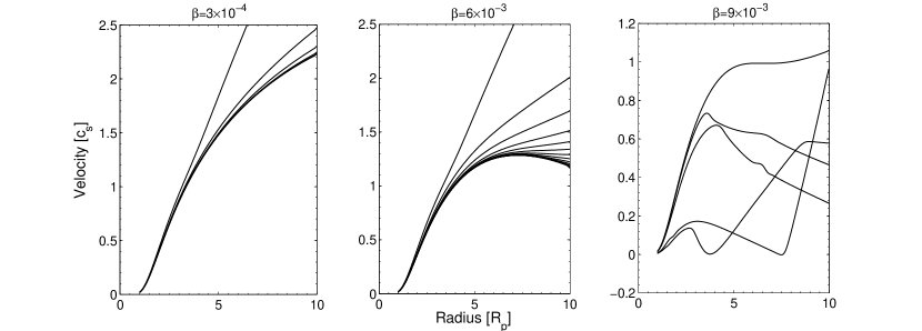
Figure 1: Snapshots of the flow velocity structure as a function of (spherical) radius from the planet for a system with $b=10$ and $\theta_{0}=0.1$. The three panels show results for magnetic field parameter $\beta_{\ast}=3\times 10^{-4}$, $6\times 10^{-3}$, and $9\times 10^{-3}$. For the two low $\beta_{\ast}<\beta_{\rm c}$ cases (left and middle panel), the snapshots are plotted every $t=3$ up to a total time of 30. For the case with high $\beta_{\ast}>\beta_{\rm c}$ (right panel), the snapshots are plotted every $t=20$ up to a total time of $t=100$. Note that this latter case does not converge to a smooth, steady-state solution (see text).

2.2 Choice of Boundary Condition

One part of the advantage of our approach is we have much more control over the implementation of the boundary conditions than in the multi-dimensional calculations (Owen & Adams, 2014). At the inner boundary the choice depends on whether the gas velocity on the boundary is inwards or outwards. If the velocity is outwards the choice is easy and the ghost cells are assigned the base density hydrostatic structure $\rho_{\rm b}$ and the velocity structure is chosen to feed the domain with the required mass-flux. If the gas velocity is inwards we have two choices: either implement outflow boundary conditions or zero mass flux boundary conditions. The former would be appropriate if any inward flow could disturb the underlying atmosphere and the latter if it could not. Since the multi-dimensional calculations which included a portion of the unheated atmosphere in the simulation domain show that any inflow that occurred was sub-sonic and therefore did not disturb the atmosphere then a zero-mass flux boundary is the more physical choice. Therefore, if we detect inflow at the inner boundary the velocity is set to zero and we retain the hydrostatic density structure in the ghost zones.

For the outer boundary again the choice of boundary condition depends on whether the gas velocity is inflowing our outflowing. In the case of outflow we use outflow boundary conditions. However, due to the fact the outflow velocity is often sub-sonic standard extrapolations techniques employed often lead to spurious reflections from the outer boundary, which propagate back into the simulation domain and lead to non-physical flow structure developing. Instead we apply characteristic tracing boundary conditions (Thompson, 1987), where the values in the ghost zones are computed assuming that only outgoing characteristics at the boundary and any incoming characteristics are given zero amplitude. This prevents any spurious reflections and the details of our implementation is detailed in the Appendix. In the case we detect inflow at the outer boundary we set the velocity to zero and the density to the ambient value due to the presence of the star’s wind/atmosphere (i.e., $\rho=10^{-6}\rho_{\rm b}$), although we note that the choice of this value has little effect on the dynamics unless it is comparable to the hydrostatic value.

3 Transition to Non-steady Flow and Time Variability

For a given magnetic field line, there exists a critical value of the background stellar field (specified as $\beta_{\rm c}$), above which no steady-state solutions exist that satisfy the required boundary conditions (i.e., $\rho\rightarrow 0$ as $r\rightarrow\infty$). This claim includes hydrostatic solutions. As a result, the only possible outflows must display non-steady (time-varying) flow. Moreover, the critical value of the magnetic field strength ratio ($\beta_{\rm c}$) is predicted by analytic theory (Adams, 2011). To demonstrate this transition, from systems that allow steady-state flow to those that do not, we construct a set of simulations where we increase $\beta_{\ast}$ from below $\beta_{\rm c}$ to above.

For high launching latitudes, the critical, $\beta_{\ast}$ is given by $\beta_{\rm c}\approx 8/b^{3}$ (Adams, 2011). For our “standard” set of simulation parameters, we choose $b=10$ and $\theta_{s}=0.1$, so that the critical value $\beta_{\rm c}\approx 0.008$. In Figure 1, we show snapshots of the velocity structure for flows with $\beta_{\ast}=0.0003$, 0.006 and 0.009. For the two lowest $\beta_{\ast}$ values (shown in the left and middle panels), we find that the velocity structure approaches the steady-state transonic wind, passing smoothly through a sonic point on a time-scale of order several sound crossing times. For the simulation with $\beta_{\ast}>\beta_{\rm c}$, however, we find that the flow never attains a steady-state form. Instead, the flow remains highly variable, with both alternating epochs of outflow and inflow occurring over time-scales of order tens of flow time-scales. After an initial transient phase, this flow structure approaches a quasi-repetitious pattern, but no steady-state flow is found on a time-scale of 1000s of flow time-scales. This result demonstrates that when the flow cannot pass smoothly through a sonic point, no steady state solutions are allowed, and the flow must become highly variable in time (as expected).

3.1 Properties of the variability in non-driven flows

The variability in the flows with $\beta_{\ast}>\beta_{\rm c}$ settles into a quasi-repetitious flow with outflow followed by periods of inflow. We find that the time-scale associated with variability depends on the size of the domain simulated (i.e., on the radius of the outer boundary). In Figure 2, we show the surface mass-loss rate $\dot{\Sigma}$ from the planet ($\rho u$ evaluated at the planet’s surface) as a function of time for outer boundaries $R_{\rm out}$ = 10, 20 and 30 (from top to bottom). These simulations use our “standard” set of model parameters ($b=10$, $\theta_{s}=0.1$), where we use a super-critical value of the stellar background field $\beta_{\ast}=0.03>\beta_{\rm c}$.

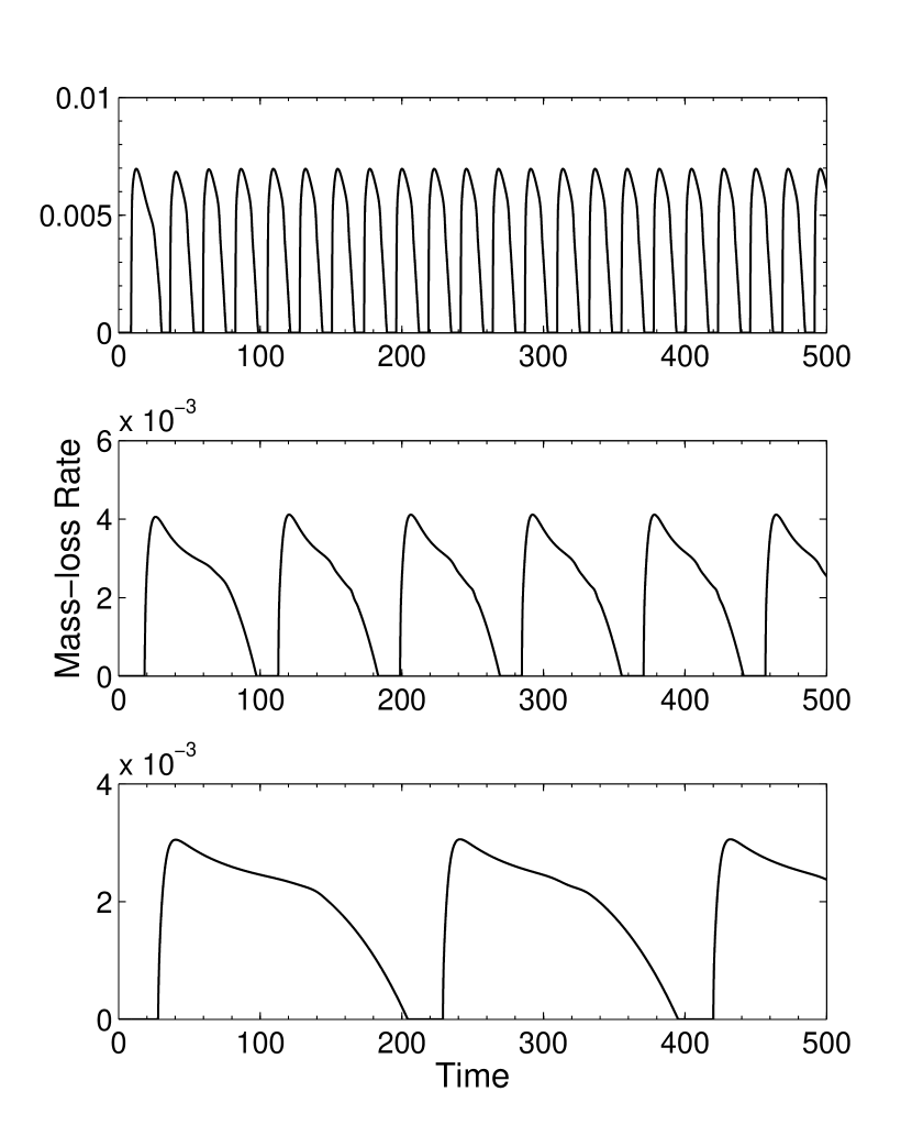
Figure 2: Surface mass-loss rate from the planet as a function of time for a system with $b=10$, $\theta_{s}=0.1$, and $\beta_{\ast}=0.03$. Panels show simulations with outer boundaries at $R_{\rm out}$ = 10, 20 and 30 (from top to bottom). Note that the variability time scale depends on the value of $R_{\rm out}$.

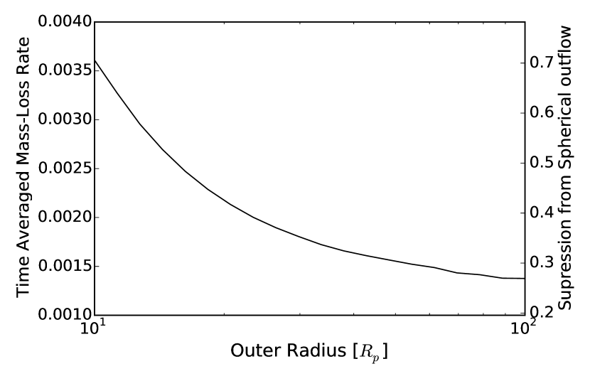
Figure 3: The time averaged mass-loss rate (in dimensionless units) as a function of outer boundary radius $R_{\rm out}$ [given here in units of $R_{\rm p}$]. The right-hand $y$-axis shows the amount by which the time-averaged mass-loss rate is suppressed compared to a spherical transonic outflow.

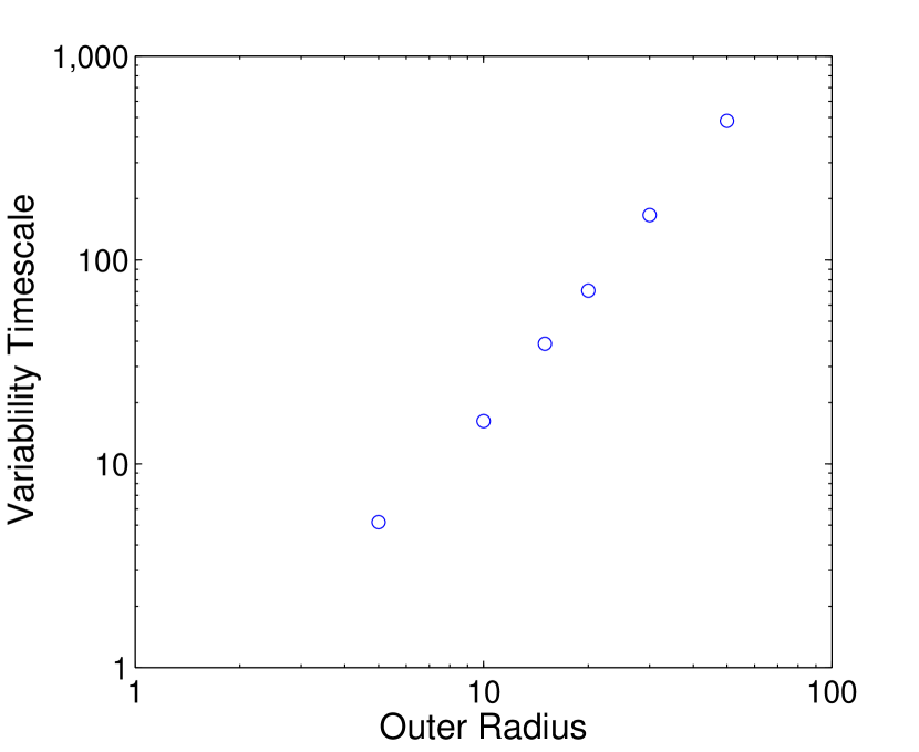
Figure 4: Variability time-scale as a function of the outer boundary radius. The variability time is define as the time interval over which $\dot{\Sigma}>0$ at the planetary surface (see Figure 2). Note that the variability time is proportional to the the square of the boundary radius.

Figure 3 shows the time-averaged mass-loss rate as a function of outer boundary radius. This plot shows that the time-averaged mass-loss rate falls steadily with increasing radius of the computational domain. On the right vertical axis, the figure also shows the mass-loss rate as a function of its value for a purely spherical outflow. The mass-loss rate is thus suppressed by a substantial factor, which varies from about 70% to only about 25 percent as the outer boundary varies from $R_{\rm out}$ = 10 to 100.

Figure 4 shows that the variability time-scale (essentially the period) strongly increases with the radius of the outer boundary. The simulations also show that the shape of the surface mass-loss rate profiles appears to be scale free and that the amplitude of the surface mass-loss profiles decreases with increasing domain size. Here we define the variability time-scale to be the time span over which the surface mass loss rate is non-zero, i.e., $\dot{\Sigma}>0$. We then plot this time scale as a function of the outer boundary radius as shown in Figure 4. This figure shows that the variability time-scale $t_{\rm evolve}$ increases as a power-law function of the outer boundary radius, where the approximate scaling law has the form $t_{\rm evolve}\propto$ $R_{\rm out}^{2}$. We note this variability time-scale is longer than the flow time-scale of the entire domain, where this latter time is typically a few $R_{\rm out}$ and obviously increases linearly with the outer radius.

3.2 Model for non-driven flows

When the flow is not driven at the inner boundary it develops a steadily repeating pattern where the flow approaches Mach numbers $\sim 1$ at the outer boundary but then decays to towards the hydrostatic solution. It passes through the hydrostatic solution and inflows until the material at large radius reaches low pressures and the outflow is launched again. We show snapshots of the velocity structure at various time-intervals in Figure 5 as thick dashed lines.

The variability time-scale is clearly longer than the flow sound crossing times for the domain $R_{\rm out}>10$. Thus one might expect it is possible to setup and maintain a steady flow, over a large part of the domain. It this regime there are no transonic solutions and the only available solutions are the breezes - which we note do not satisfy the Boundary Condition of zero pressure at large radius. These breeze solutions are plotted in Figure 5 as thin grey lines (each line corresponds to a different mass-flux), with the simulation profiles overlain for $\beta_{\ast}=0.03$, $b=10$, $R_{\rm out}=20$ and $\theta_{s}=0.1$.

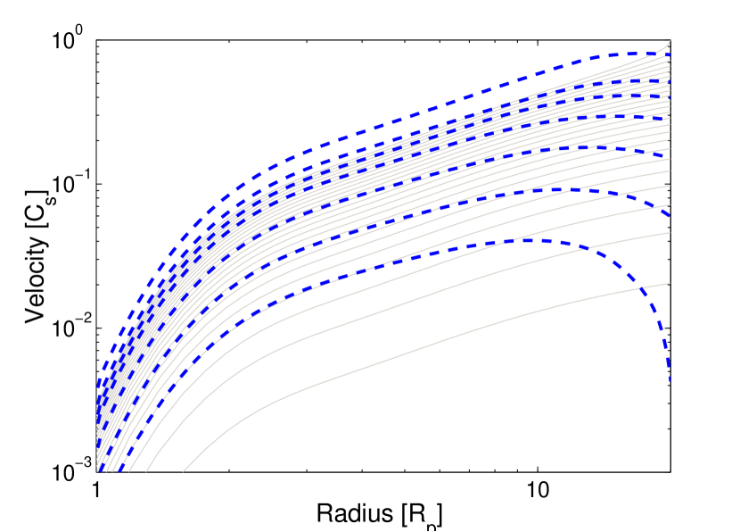
Figure 5: Velocity profiles for ‘breeze’ solutions (shown here as the thin grey lines) for systems with $\beta_{\ast}=0.03$, $\theta_{s}=0.1$, and $b=10$, with the outer boundary at 20 $R_{\rm p}$. The thick dashed lines (in blue) show snapshots of the velocity profile from a simulation with the same parameters. The velocity profile decays in time, where these snapshots are shown for times of 21.3, 29.0, 36.6, 44.3, 49.6 and 52.7 after the first (uppermost) profile.

The profiles from the simulations indicate that the flow is able to maintain nearly steady-state breeze solutions out to a region close to the outer boundary. At this boundary, however, the velocity (and hence the mass-flux) is reduced. If the the mass-flux changes near the boundary, then clearly the density near the outer boundary must also be evolving in time. Suppose that we assume that a (nearly) steady-state breeze solution exists in the inner region close to the planet; then the density at large radius, near the outer boundary, will act as the boundary condition that ‘chooses’ which of the breeze solutions is operating at a given time.

However, because the mass-flux is not constant, but rather decreases near the outer boundary, the density near the boundary must increase. Because the breeze solution ‘chosen’ depends on the density at large radius, the choice of breeze solution will change. As the mass-flux at the outer boundary is reduced and the density increases, the breeze solution evolves to cases with lower mass-fluxes. This behaviour occurs because a higher density at large radius results in a lower mass-flux. This trend can be seen starting from the steady-state equations for mass-flux and the Bernoulli potential, i.e.,

$$\rho uh_{\phi}h_{q} = \lambda$$ (14)

$$\frac{1}{2}u^{2}+\log\rho+\psi = \epsilon$$ (15)

where $\lambda$ is the mass flux and $\epsilon$ is the value of the Bernoulli potential (and where both $\lambda$ and $\epsilon$ are constants). Following Adams (2011) we can define an ancillary function $H$ such that $h_{q}h_{\phi}=q/H^{1/2}$ and

$$H=(\beta_{\ast}+2/\xi^{3})^{2}\cos^{2}\theta+(\beta_{\ast}-1/\xi^{3})^{2}\sin^{2}\theta\,.$$ (16)

Applying our dimensionless boundary conditions that $\rho=1$ and $u=u_{1}$ at the planet’s surface with radius $\xi=1$, and taking $\rho=\rho_{\rm out}$ at the outer boundary $\xi=R_{\rm out}$, Equations (15) can be solved to derive an expression for $\rho_{\rm out}$ in terms of the dimensionless mass flux $\lambda$,

$$\rho_{\rm out}=\frac{\lambda H_{\rm out}^{1/2}}{q}\frac{1}{\cal D}\,,$$ (17)

where we have defined

$${\cal D}\equiv\sqrt{-W_{0}\left[-\lambda^{2}H_{\rm out}/q^{2}\exp\left(-b/R_{\rm out}+b-\lambda^{2}H_{1}/2q^{2}\right)\right]}\,,$$

where $W_{0}$ is the Lambert $W$-function. The solution to Equation (17) is plotted in Figure 6, where $\rho_{\rm out}$ is scaled to the hydrostatic value, i.e., the value corresponding to no outflow and $\lambda=0$; the other system parameters are taken to be $\beta_{\ast}=0.03$, $\theta_{s}=0.1$, and $b=10$, with the outer boundary located at $R_{\rm out}=20$.

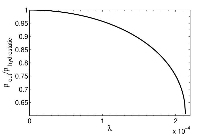
Figure 6: Density at the outer boundary as a function of dimensionless mass-loss rate $\lambda$, from the solution to Equation (17), for $\beta_{\ast}=0.03$, $\theta_{s}=0.1$ and $b=10$ with $R_{\rm out}=20$. No solution exists for sufficiently large mass-loss rate $\lambda>2.1351\times 10^{-4}$, which corresponds to $u=c_{\rm s}$ at the outer boundary.

.

As shown in Figure 6, a larger density $\rho_{\rm out}$ at the outer boundary results in a lower mass-flux $\lambda$. Given this dependence, we argue that breeze solutions with one-way outer boundaries (such that material can flow outward, but not back inwards) are subject to an instability. Consider a steady state ‘breeze’ solution that causally connects the outer boundary and planet’s surface. If one perturbs the mass-flux at large radius on a time-scale longer than the flow time-scale, this action will result in a density change at large radius due to mass continuity. Since $\rho_{\rm out}$ is a monotonically decreasing function of $\lambda$, this process will be unstable: Suppose that the perturbation increases the density at large radius; the resulting mass flux will tend to follow the curve in Figure 6 and hence decrease, which will increase the density even further. We suspect that this instability is similar to the one described by Velli (1994); Del Zanna et al. (1998) for sub-sonic spherical outflows, resulting in a hysteresis-like cycle of outflow and inflow.

Taking this instability to be the cause of the cycle seen in our simulations, one can build a simple model that aims to reproduce the time-scale of variation and the self-similar mass-flux profile, along with its amplitude as seen in Figure 4. Toward this end, we can write the mass contained in the flow at large radius in the form:

$$M_{\rm out}\propto\int^{t}\lambda\,{\rm d}t\,.$$ (18)

If we now assume that the decrease in mass-flux is sensitive to the outer boundary, then the region over which the flow ‘feels’ the outer boundary should be comparable to the scale height in the flow (denoted here as $L_{\rm s}$). Equation (18) can be rewritten as:

$$\rho_{\rm out}h_{q}(R_{\rm out})h_{\phi}(R_{\rm out})L_{\rm s}(R_{\rm out})\propto\int^{t}\lambda\,{\rm d}t\,.$$ (19)

We can turn the above expression into a differential equation for the evolution of $\rho_{\rm out}$ simply by taking the time derivative, so that it becomes:

$$\frac{d\rho_{\rm out}}{dt}h_{q}h_{\phi}L_{\rm s}\propto\lambda\,.$$ (20)

Since $\lambda$ depends on the density at the outer boundary through Equation (17), one can find a single differential equation to solve for the evolution of $\rho_{\rm out}$.

Equation (20) can be solved numerically. However, for non-zero values of $\beta_{\ast}$, and for large boundary radii where $R_{\rm out}\gg 1$, Equation (17) is actually roughly independent of $R_{\rm out}$. Note that the $b/R_{\rm out}$ term is small compared to $b$, and that at large radius $H_{\rm out}$ approaches a constant value:

$$H\rightarrow\beta_{\ast}^{2}\quad\mbox{ as }\quad\xi\rightarrow\infty\,.$$ (21)

This limiting form arises because the magnetic field lines are the nearly vertical with zero divergence at large radius (as they are dominated by the stellar background contribution). This result is not surprising, in that the domination of the stellar background field is the origin of the complication that that transonic flows do not exist in the first place.

In the limiting regime described above, the density $\rho_{\rm out}$ is almost purely a function of the dimensionless mass flux $\lambda$. The differential equation itself can easily be made dimensionless, allowing us to extract a time-scale scaling with $R_{\rm out}$. Noting $qH^{-1/2}=h_{q}h_{\phi}$, we find that the $h_{q}h_{\phi}$ term on the left-hand-side of the differential equation cancels. The time-scale for the evolution of the differential equation is then given by:

$$t_{\rm evolve}\sim L_{\rm s}\,.$$ (22)

Since the breezes are sub-sonic, the density structure of the flow can be considered as nearly hydrostatic, which implies that the scale height is given approximately by:

$$L_{\rm s}(R_{\rm out})=\left|\frac{\partial\log\rho}{\partial r}\right|^{-1}=|g|^{-1}=R_{\rm out}^{2}/b\,.$$ (23)

Thus, the $R^{2}$ dependence of the time-scale comes from the fact the scale height at large radius scales as $R^{2}$ and the background stellar field forces the stream-bundle area to be constant. Notice also that — in addition to the scaling — the absolute value for the variation time-scale is comparable to that found in Figure 4 for $b=10$. For completeness, we note that the scale height in equation (23) does not take into account the geometry of the magnetic fields. In the limit $\xi\gg 1$, the field lines are nearly vertical, and the scale height should be corrected by the geometrical factor $\xi/z$. In the extreme limit, however, $\xi/z\to 1$, so we can ignore this complication.

Curiously, because the scale height increases as $R_{\rm out}^{2}$, for sufficiently large domain sizes $R_{\rm out}$ the evolution time is longer than the sound crossing time of the flow, where $t_{\rm cross}=R_{\rm out}$ in dimensionless units. This finding suggests that only a fraction of the flow will be able to adjust during a crossing time, where this fraction is given by $f=t_{\rm cross}/t_{\rm evolve}=b/R_{\rm out}$. For the case of our example shown in Figure 5, this fraction $f=1/2$. Note that the flow profiles from the simulation match onto the breeze solutions for the inner half of the domain and diverge from the breeze solutions in the outer half.

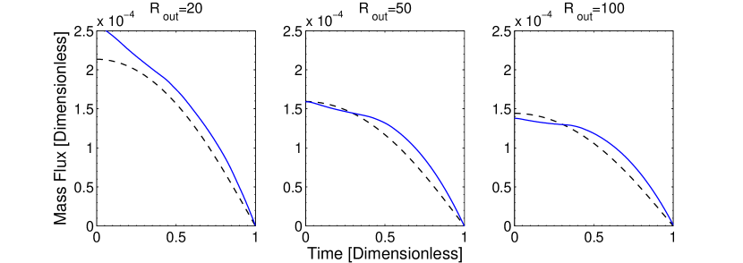
Figure 7: Evolution of mass-flux versus time for numerical calculations (solid curve) and a simple model described in the text (dashed curve). The time variable (horizontal axis) is scaled so that the total time evolution is unity in all cases.

A final test is to predict the evolution of time-varying outflow solution as it evolves by sampling through various breeze solutions; we would also like to understand the amplitude of these variations. In the limit $R_{\rm out}\gg 1$, the solution must become self-similar, as the $b/R_{\rm out}$ term can be dropped and quantity $H_{\rm out}$ approaches a constant. Assuming that the solution starts with speed $u_{\rm out}=1$, we can numerically integrate the differential equation to find the time evolution of the mass-flux ($\lambda$). The solutions are plotted in Figure 7 for several values of $R_{\rm out}$; these results are compared to the numerical solutions, for which the mass flux $\lambda$ is measured at $R_{\rm out}/2$. The agreement is good, in both amplitude and evolution. We can also check the time-evolution for different values of $q$ and $\beta_{\ast}$; the solutions should independent of these values, provided the systems are in the regime which does not allow transonic flow. Which indeed we find with $\beta_{\ast}$ range 0.02 to 0.2 and $\theta_{s}$ in range 0.01 – 0.2.

The discussion above indicates that the origin of the time-variability in undriven magnetically controlled flow is an instability in the breeze solutions; moreover, the time-scale of the variations is set by the scale height at the outer boundary such that $t_{\rm evolve}$ $\propto R_{\rm out}^{2}$. Note that since the velocity is not zero at the outer boundary, one must write Equation (20) as a scaling relation rather than an equality. All of the subsequent analysis assumes that the relevant constant is roughly independent of the parameters of the simulation. The simulations seem to suggest that this is true. We hypothesis that are full linear analysis of the global modes of any instability might give further insight. Since this type of work has not been performed for even simple spherical outflows due to the lack of obvious basis functions (for a discussion of possible approaches to spherical breezes, see Theuns & David 1992), we shall not attempt such an analysis here.

4 Driven Flow

Time variations in the outflow can arise for two conceptually different reasons. In the first case, as outlined in the previous section, time dependent flow arises when the fluid cannot pass smoothly through a sonic transition (and this type of time variation occurs even for steady heating). In addition, planets can also experience external variability, so that outflows can be time dependent due to external factors. In this case, the time scale of the variability will be linked to the driving mechanism. Possible sources of such driving variations include stellar flares or outbursts, and/or an eccentric orbit that modulates the flux of UV and X-ray radiation received by the planet. Any modulation in the flux will change the density at the base of the outflow. For simplicity, we consider two types of driving: Sinusoidal driving and pulsed driving, where we vary the density at the base of the flow (in the ghost zones) as a function of time.

4.1 Sinusoidal Driving

To illustrate the effects of driven, time-dependent forcing, we consider the following simple model where the density at the base of the flow varies as:

$$\rho_{\rm b}=A\sin^{2}\left(\frac{t}{T_{\rm var}}\right)+1\,,$$ (24)

where $A$ is the amplitude of the variation and $T_{\rm var}$ is the time-scale on which it occurs.

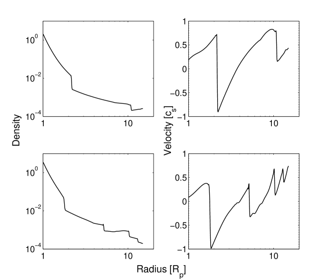
Figure 8: The density (left panels) and velocity (right panels) structure of the flow for a variability time-scale of $T_{\rm var}=2$ (top) and $T_{\rm var}=1$ (bottom). The simulation parameters are $b=10$, $\beta_{\ast}=0.01$, $\theta_{0}=0.1$, and the domain has an outer radius $R_{\rm out}$ = 15.

We have performed a collection of numerical simulations using Equation (24) as an inner boundary condition. After some initial transients, the flow settles into a quasi-repetitious pattern. Figure 8 shows snapshots of the density and velocity structure of outflows with variation time scale $T_{\rm var}=2$ (top panels) and $T_{\rm var}=1$ (bottom panels). The  flow structures depicted in Figure 8 show some generic features that are present in all of the simulations. Both the density and the velocity distributions show a series of discontinuities that originate as weak shocks near the planet and then propagate outwards.

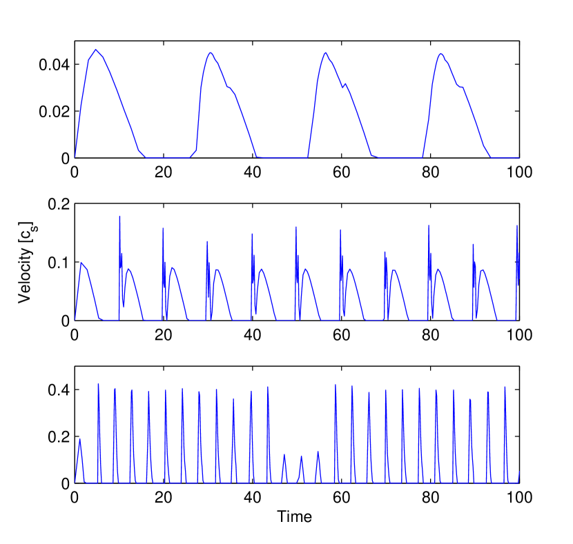
Figure 9: Velocity at the planet surface as a function of time for time-varying, driven flow with amplitdue $A=3$ and time scale $T_{\rm var}$ = 8.25 (top), 3.83 (center), and 1.78 (bottom). The system parameters are taken to be $\beta_{\ast}=0.03$, $\theta_{s}=0.1$, and $b=10$.

We now turn our attention to the outflow properties as a function of the driving time-scale $T_{\rm var}$. In Figure 9, we show how the velocity at the planet various with time for three different driving time-scales of $T_{rmvar}$ = 8.25, 3.83, 1.78. The figures shows that the amplitude of the velocity variations decreases with increasing variation time-scale (note the different scales on the vertical axis in the three panels). Furthermore, while the time-scale of the velocity variations is direct mapping of the driving time-scale, the profiles are not symmetric. For the fastest driving time-scale (1.78, bottom panel), after a time of roughly 50 the amplitude of the variation drops by a factor of $\sim 3$ and this variations of a time-scale of 50 exists for the entire simulation (over a time of several 1000s).

In Figure 10 we show the time-averaged surface mass-loss profile for a range of driving time-scales in the range $T_{\rm var}=0.1-10$, where the averaging has taken place over a simulation time of 500. As shown in the Figure, the time-averaged mass loss rate is relatively constant as a function of the driving time for the regime where $T_{\rm var}<1$, and decreases for larger values of $T_{\rm var}$. More specifically, the mass loss rate displays a moderate peak near $T_{\rm var}\approx 1$, and decreases according to $1/T_{\rm var}$ for large driving time scales.

We can understand the behaviour shown in Figure 10 as follows. For small values of the driving time, smaller than the sound crossing time, the flow cannot adjust to the changing driving density. As a result, in this regime the driving density (see equation [24]) can be effectively replaced with a time-averaged value. However, the numerical simulations also show that the flow is not able to cycle through its low-mass-loss states, as it does in the case of truly constant base density (see Figure 2). As a result, the mass loss rate is more nearly constant in time (instead of showing periodic behaviour) and the time-averaged value is correspondingly higher. In the opposite regime, where the driving time scale is much longer than the crossing time, the flow has time to adjust and reach its low states, so that the mass loss rate decreases. In addition, the driving density (see equation [24]) is only larger than its baseline value (chosen here to be unity) for a fraction of the time, where the fraction $\propto 1/T_{\rm var}$.

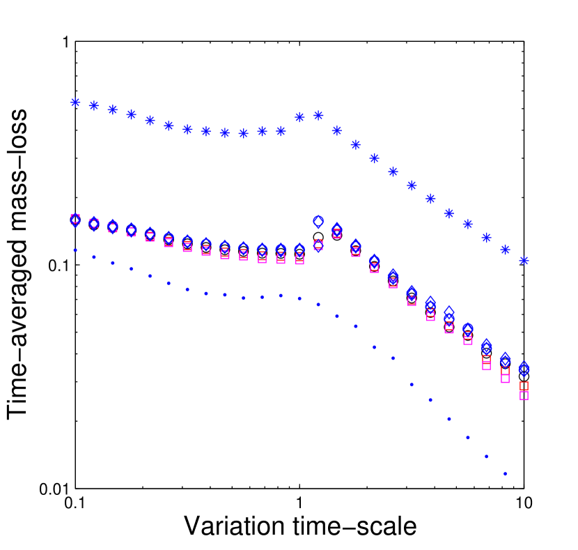
Figure 10: The time-averaged mass-loss rate as a function of driving time-scale. The open points show results for $b=10$ and $A=3$, where the other parameters are allowed to vary. The stars show our “standard” model but with $A=10$ (upper curve), whereas the dots show our standard model but with $b=15$ (lower curve).

In Figure 10, the points show simulation results with $b=10$ and $A=3$ held fixed and varying values of $\beta_{\ast}$ and $\theta_{s}$. The stars stars show our “standard” case but with an increased amplitude of $A=10$; the dots show simulations with $b=15$. We note the profiles are somewhat similar and have a power-law fall-off once the variation-time-scale is greater than unity, where the time-averaged mass-loss rate can approximately be described as $\propto T_{\rm var}^{-1}$.

4.2 Pulsed Driving

Another possible source of driven time variations is UV and X-ray heating from stellar flares. These bursts of radiation could act to heat the upper layers of the planetary atmosphere and thereby increase the density at the base of the outflow. Flares act in a pulsed manner, which can be characterized by a time scale $\Delta_{T}$ over which the radiation is enhanced and by an amplitude $A_{p}$ that specifies the degree of enhancement. In this set of simulations, we also let the pulses repeat on a time-scale of $t_{\rm var}$. In Figure 11, we show a snapshot of the flow properties for our “standard” set of parameters with $\Delta_{T}=0.1$ and $t_{\rm var}=1$.

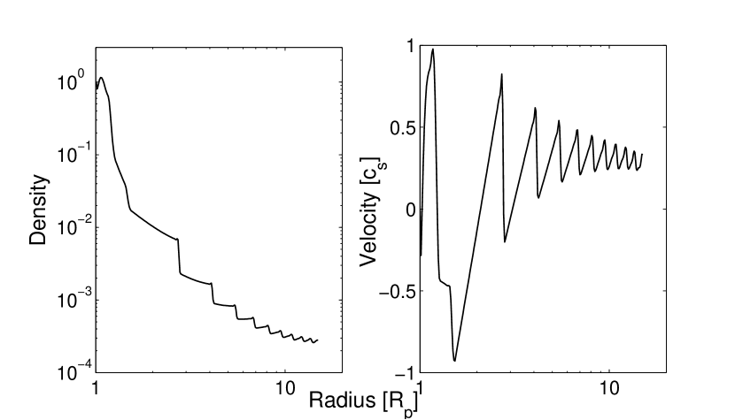
Figure 11: The density (left panel) and velocity (right panel) structure of the outflow for pulsed driving. The variability time-scale $t_{\rm var}=1$ and the pulse duration $\Delta_{T}=0.1$. The simulation parameters are $b=10$, $\beta_{\ast}=0.01$, and $\theta_{0}=0.1$, with an outer radius of the domain at $R_{\rm out}$ = 15.

We note that this figure shows significant similarities with the flow variations arising from the sinusoidal driving case discussed in the previous subsection. Specifically, discontinuities in the flow develop close to the planet due to weak shocks and then propagate outwards. As a result, the qualitative features we can expect in the case of driven flow are not particularly sensitive to the exact form of the driving, but depend primarily on the driving time-scale.

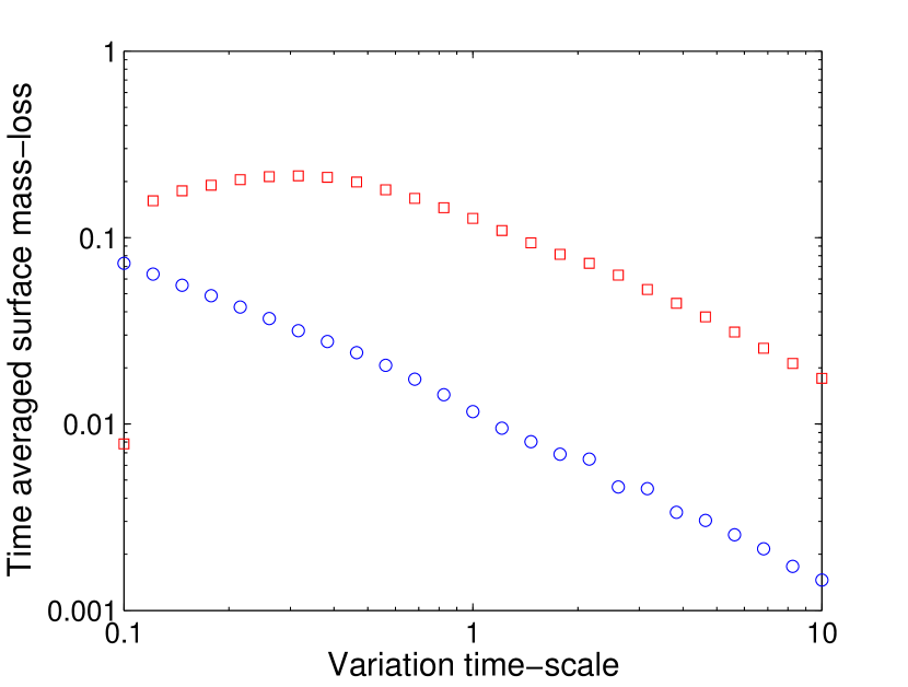
Figure 12: Time averaged mass-loss rates for the case of pulsed driving terms for pulse durations of $\Delta_{T}=0.1$ (red squares) and $\Delta_{T}=0.01$ (blue circles). Mass-loss rates are shown as a function of the time scale $t_{\rm var}$ on which the pulses repeat.

Once again we turn our attention to the general outflow properties as a function of the driving time-scale, here the time $t_{\rm var}$ on which the pulses repeat. Figure 12 shows the time-averaged surface mass-loss rate as a function of the variation time-scale $t_{\rm var}$ for systems driven with pulses of duration $\Delta_{T}=0.1$ (red squares) and $\Delta_{T}=0.01$ (blue circles). As shown in the figure, when the driving time-scale is significantly longer than $\Delta_{T}$, we see an approximate power-law fall off in time-averaged mass-loss rate with variation time-scale. This variation can be approximated as a power-law of the form $\propto\Delta_{T}^{-1}$, analogous to the behavior found for sinusoidally driven flows.

5 Implications

5.1 Flow Regimes for Observed Exoplanets

For the case of magnetically controlled flow, the magnetic field topology can prevent the flow from attaining a steady-state solution, in part due to the inability of the flow to pass smoothly through the sonic transition. This regime arises for magnetically controlled evaporation of close-in exoplanets when the background stellar field is sufficiently strong. For the case of anti-aligned dipoles on the star and planet, the criterion for unsteady outflow (Adams, 2011) is given by the expression

$$\frac{B_{*}}{B_{\rm p}}\left(\frac{R_{*}}{a}\right)^{3}\left(\frac{GM_{\rm p}}{R_{\rm p}c_{\rm s}^{2}}\right)^{3}=\beta_{\ast}{b^{3}}\gtrsim 8\,.$$ (25)

For a Hot Jupiter orbiting a Sun-like star with surface field strength $B_{*}\approx 1$ G in a 3 day orbit, we find that variable magnetically controlled outflow will arise when the planetary field falls below the limit:

$$B_{\rm p} \lesssim 0.4~{}{\rm G}~{}\left(\frac{B_{*}}{1~{}\mbox{G}}\right)\left(\frac{R_{*}}{1~{}{\rm R}_{\odot}}\right)^{3}\left(\frac{a}{0.04~{}{\rm AU}}\right)^{-3}$$ (26)

$$\times \left(\frac{M_{\rm p}}{1~{}{\rm M_{J}}}\right)^{3}\left(\frac{R_{\rm p}}{1.4~{}{\rm R_{J}}}\right)^{-3}\left(\frac{c_{\rm s}}{10~{}{\rm kms}^{-1}}\right)^{-6}\,.$$

Simulations carried out previously (Owen & Adams, 2014) indicate that magnetically controlled flow will arise for planetary field strengths $B_{\rm p}\gtrsim 0.1$ G. The window for evaporating planets where the planetary field is simultaneously strong enough for magnetically controlled flow and weak enough for the stellar background field to compromise steady-state flow is thus 0.1 G $\lesssim B_{P}\lesssim$ 0.4 G. Time-variations will thus arise for planets in orbit around older main-sequence stars when the planetary field is moderately weak, or when the planet is extremely close to the star.

On the other hand, for a young Hot Jupiter around a pre-main-sequence Sun-like star (of age $\sim$ 1-10 Myr), the stellar magnetic fields are typically much stronger, $B_{\ast}\sim 1$ kG (e.g., Johns-Krull 2007). The above criterion indicates that the flow will be time-variable for planetary field strengths $B_{\rm p}\lesssim 475$ G. For young star/planet systems, a great deal of parameter space exists for which the planetary field is strong enough to control the flow, but weak enough so that the stellar background field dominates enough to compromise steady-state solutions. As a result, evaporating planets around young stars are likely to experience variability of the kind we describe here.

We compare the criterion for magnetically controlled evaporation variability given in Equation (25) to the exoplanet data in Figure 13. Specifically, we plot the ratio of the semi-major axis to the stellar radius against the escape velocity ($\sqrt{GM_{\rm p}/R_{\rm p}}$) for a collection of observed exoplanets (where the observational values are taken from the Open Exoplanet Catalogue on 31/08/2015; Rein 2012). The figure shows lines of constant stellar-to-planetary surface magnetic field strength, where the ratio has the value 0.3 (solid), 1.0 (dashed), 3 (dotted), and 10 (dot-dashed). Planets that lie below the line (for a given field strength ratio) could be prone to variability. Note that for early evolutionary times, the planets will have larger radii (as planets cool and shrink with time), so that the points will move to the left for younger planet populations.

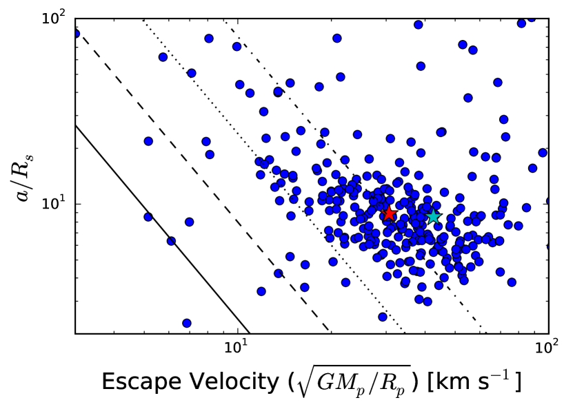
Figure 13: The ratio of semi-major axis to stellar radius plotted against the escape velocity from the planetary surface for observed exoplanets (shown as points). The lines show a constant stellar to planetary surface magnetic field strengths (0.3 – solid, 1 – dashed, 3 – dotted, and 10 – dot-dashed) assuming sound speed $c_{\rm s}=10$ km s^-1. For a given ratio of field strengths, planets that fall below the line are susceptible to non-steady-state outflows. The star symbols represent currently observed evaporating Hot Jupiters HD 209458b (red) and HD 189733b (cyan).

Figure 13 shows that if Hot Jupiters have strong enough magnetic fields to be magnetically controlled, $B_{\rm p}\gtrsim 0.1$ G (Owen & Adams, 2014), then a significant fraction of them are likely to experience time-dependant evaporation. However, we note that the two observed evaporating planets HD 209458b and HD 189733b (marked by stars in Figure 13) are unlikely to be experiencing variability of this kind. In order for the planets to have weak enough magnetic fields for a 1 gauss stellar field to produce the required ratio, the planetary field would be too weak to control the flow; alternately, the high ratio of stellar to planetary field could be achieved by strong fields on the stellar surface, but they are rare.

Since stellar magnetic fields are expected to be considerably larger at early times, up to 1000 times stronger, we suspect that almost all Hot Jupiters will experience evaporation variability of this kind provided the flow is magnetically controlled.

5.2 Physical time-scales

For convenience, almost all of the work in this paper has been performed in dimensionless units. In order to discuss observational implications, however, we must consider typical physical parameters for the systems of interest. Here we consider separately the two regimes of variability, those for undriven and driven outflows.

5.2.1 Undriven flow

For undriven flow we found that the time-scale for variability in dimensionless parameters is $R_{\rm out}^{2}/b$, which can be written in physical variables in the form:

$$t_{\rm var}=\frac{R_{\rm out}^{2}c_{\rm s}}{GM_{\rm p}}\approx 6~{}\mbox{h~{}}\left(\frac{R_{\rm out}}{20R_{\rm J}}\right)^{2}\left(\frac{c_{\rm s}}{10~{}\mbox{km s}^{-1}}\right)\left(\frac{M_{\rm p}}{1~{}{\rm M}_{J}}\right)^{-1}\,.$$ (27)

Obtaining the actual time-scale depends on specifying the choice of the ‘outer boundary’. In conceptual terms, the outer boundary of the flow regime is set by the outer boundary of the effective sphere of influence of the planet. Given that the flow is magnetically controlled, one sensible choice would be the radius at which the stellar magnetic field starts to curve back towards the star and can no longer be considered approximately vertical. This transition will occur on a length scale of $(a/R_{*})R_{\rm p}$, which falls in the range of $5-100$ times the planetary radius. The corresponding time scales for such boundary radii vary from a few hours to a few days, variability times that are eminently observable.

Another choice for the outer boundary scale is the radius at which the planetary wind becomes entrained in the stellar wind: When the outflow from the planet is sufficiently far from the surface, the ram pressure of the stellar wind will dominate that of the planetary outflow, and the latter will be blown away. Owen & Adams (2014) estimated that this radius to occur at approximately $10-20R_{\rm p}$ for typical stellar wind parameters. The corresponding time scales for flow variability are once again in the range of a few hours to a few days.

For both cases considered above, the variability time-scale time scales ranges from a few hours to a few days. The short end of the range is roughly comparable to the transit duration and the long end of the range is roughly comparable to the orbital period (for a Hot Jupiter). Given this ordering of time scales, one would expect the evaporative flow to vary from transit to transit.

5.2.2 Driven flow

Driven flow can arise when the high energy flux of radiation received by the planet displays time-variability. This paper has considered the specific case where this variability results in a time-variable base density that drives the flow. As discussed in Section 4, the response of the planetary evaporation depends on whether the driving time-scale is shorter or longer than the planet sound crossing time-scale ($R_{\rm p}/c_{\rm s}\approx 3$ hours). If the driving time is shorter than the crossing time, the flow cannot respond to the rapid variations. As a result, the bulk quantities of the flow are largely unchanged, as the fluid cannot globally respond on a time-scale shorter than the flow crossing time. On the other hand, if the driving time is longer than the crossing time, the fluid does have time to respond; the density and velocity distributions will thus vary on the driving time scale. In addition, the time-averaged mass-loss rate follows an approximate power-law decline with increasing variability time-scale.

Hot Jupiters have (at least) two obvious sources of flux variability that can affect evaporation, including an eccentric orbit and/or stellar flares. An eccentric orbit will lead to flux variability on a time scale comparable to the orbital period, which is typically a few days in these systems. In addition, stellar flares are observed to vary on time scales of order a few hours to a few days (Güdel et al., 2003). As as result, we expect that most driven flows will have a response firmly in the regime where the variability is longer than the planet sound crossing time. The variability thus leads to a net decrease in the time-averaged mass loss rate (see Figure 10). In addition, with a variability on a time-scale of a few hours to days, we expect the flow to vary from transit to transit. This indeed maybe the case for HD 189733b, where Lecavelier des Etangs et al. (2012) identified temporal variations in the Lyman-$\alpha$ absorption between two different epochs. As discussed above, the expected stellar and planetary magnetic field strengths mean spontaneous variability driven by the magnetic topology is unlikely. However, an X-ray flare was seen several hours before one of the transits with a factor 2-3 increase in flux. Our driven simulations show that variability of the high-energy flux on a time-scale of several hours ($T_{\rm var}\sim 1$), could lead to significant variability in the flow (see bottom panel of Figure 8). Thus, the X-ray flare could be responsible for the variability seen in the outflow of HD 189733b as hypothesised by (Lecavelier des Etangs et al., 2012).

Targeted observations of known eccentric planets, or co-eval observations in the X-rays to detect flares, could thus be used to study driven variability; this would be particularity useful in the case of the HD 189733 system as contemporaneous interactions between flares and outflow are already indicated.

5.3 Implications of observing variability

Since the presence of any time variations in the flow is directly linked to the strength of the planetary magnetic field, the results of this paper provide an intriguing opportunity to place constraints on the magnetic field strengths of exoplanets. For example, such a constraint could be found by producing a diagram similar to Figure 13 and looking for the transition between planets which show variability and those which do not.

Understanding the origin of inflated Hot Jupiters remains an unsolved problem (e.g., Laughlin et al., 2011). In one of the currently favoured explanations, inflation arises from ohmic heating due to energy dissipation from planetary winds interacting with the planetary magnetic field (e.g., Batygin & Stevenson, 2010). In this case, the planetary magnetic field strength is a key parameter and theoretical models tend to favour relatively large field strengths ($B_{\rm p}$ $\gtrsim$ 10 gauss) in order to account for the observed planetary radii (e.g., Batygin & Stevenson, 2010; Batygin et al., 2011; Menou, 2012). One should keep in mind that ohmic dissipation occurs at much deeper layers in the planetary atmosphere than the launch of outflows, as considered in this paper. Nonetheless, both physical processes are tied to the strength of the magnetic field strength at the planetary surface. As a result, detections of flow variability consistent with magnetically controlled outflows could be used to place constraints on the field strength and hence level of ohmic dissipation.

6 Conclusion

This paper has considered magnetically controlled outflows from Hot Jupiters in the regime where the magnetic field configurations do not allow the flow to pass smoothly through the sonic point. In this regime, the resulting outflows are necessarily time-varying. Here we present a summary of our main results, a brief discussion of their implications, and some recommendations for future work.

6.1 Summary of Results

[1] We have developed a scheme to consider the flow along a particular magnetic field line, where the flow geometry (including, e.g., the divergence operators) are taken into account using coordinate systems developed in earlier work (Adams, 2011). The numerical results show that a critical value of $\beta_{\rm c}$ exists, where $\beta_{\ast}$ is the ratio of the stellar field strength to the planetary field strength, where both are evaluated at the planetary surface. Systems with larger $\beta_{\ast}>\beta_{\rm c}$ have open magnetic field lines, and hence open streamlines, for which the flow cannot pass smoothly through the sonic point. For these cases, steady-state solutions do not exist and the flow must be time variable. Moreover, the critical value $\beta_{\rm c}$ found numerically (Section 3) is in good agreement with that derived in the previous analytic treatment of the problem (Adams, 2011).

[2] For the case of steady-state forcing (due UV heating from the star), we have found the corresponding time-dependent flow solutions. These solutions exhibit quasi-periodic behaviour (see Figure 2). The time scale (essentially the period) of these variations depends on the location of the outer boundary (see Figure 4). This dependence on the domain size arises because the flow remains subsonic, so that information can propagate inward from the outer boundary and affect the flow. In real planetary systems, the location of the effective outer boundary for the planetary outflow is determined by the interface between the sphere of influence of the planet and that of the star (Owen & Adams, 2014; Adams, 2011). In dimensionless units, the time scale of the variations is given by $T_{\rm evolve}\sim R_{\rm out}^{2}/b$, which corresponds to the sound-crossing time of the scale height of the flow evaluated at the outer boundary (see equation [23]).

[3] To elucidate the physics of these time-varying, subsonic, magnetically-controlled flows, we have also considered systems where the driving (heating) function is time-varying. This complication is implemented by forcing the density at the base of the flow to be time dependent, where we consider both sinusoidal and impulse approximations. For the sinusoidal case, the driving function is determined by an amplitude $A$ and a time scale $T_{\rm var}$. The time-averaged mass loss rate depends on the ratio of the driving time scale $T_{\rm var}$ to the sound crossing time of the planet. For short driving time scales, $T_{\rm var}\ll 1$, the sinusoidal variations are effectively averaged out, and the time-averaged mass loss rate is nearly constant as a function of $T_{\rm var}$. In the opposite limit, where the driving time scale is long, $T_{\rm var}\gg 1$, the flow has time to adjust and is only driven for a fraction of the time; this complication leads to the time-averaged mass loss rate decreasing with the driving time. In the cross-over regime, where $T_{\rm var}\sim 1$, the mass loss rate displays a moderate resonant enhancement (see Figure 10).

[4] The case of pulsed driving leads to similar behaviour. The time-averaged mass-loss rate is nearly constant as a function of the pulse separation time for $t_{\rm var}\lesssim 1$, and decreases with increasing $t_{\rm var}$ for larger values (see Figure 12).

[5] The time variations in the flow are potentially observable, and the considerations of this work can predict the relevant time scales (which vary from a few hours to a few days). For the simplest case where the heating is steady, but the flow cannot pass smoothly through the sonic point, the outflow displays quasi-periodic behaviour with a time scale that depends on the effective size $R_{\rm out}$ of the outflow cavity (equation [27]). This size scale is set by the outer boundary of the sphere of influence of the planet and depends on the magnetic field strength of the planet, as well as the stellar outflow and magnetic field parameters (this regime is determined by the size of the dimensionless fields defined in Owen & Adams 2014). With enough data, this line of inquiry can be used to constrain the magnetic field strength on the planet by measuring the time scales.

[6] For the existing sample of close-in exoplanets, and for typically expected values of the magnetic field strengths, planetary outflows are almost always magnetically controlled by a safe margin (see also Adams 2011; Owen & Adams 2014). Most planets orbiting older (main-sequence) stars are likely to achieve steady-state transonic outflows, but some fraction of evaporating planets are predicted to display time-dependence (see Figure 13). For younger (pre-main-sequence) stars, where stellar magnetic field strengths $B_{\ast}\sim 1$ kG, a much larger fraction of planetary systems are likely to experience time-variations in their outflows of the type considered in this paper.

6.2 Discussion and Future Work

The problem of planet evaporation separates into two regimes. Physical processes in the inner region near the planet determine the launch of the outflow from the planetary surface. In the present setting, the geometry of the flow in this inner region is controlled by planetary magnetic fields; the stellar background field also affects the flow geometry and can prevent sonic transitions, where this complication leads to time variability. The outflow must eventually leave the sphere of influence of the planet and enter into an outer region that is dominated by external factors, including the stellar wind and the stellar magnetic field. The nature of the flow in this outer region will depend on the ratio of the ram pressure of the stellar wind to the pressure of the stellar magnetic field, where both are evaluated near the location of the planet. The outer boundary of the inner region (equivalently, the inner boundary of the outer region) sets an important length scale in the problem, where this scale is represented by the outer boundary $R_{\rm out}$ of the simulations in this paper. For example, this boundary radius determines the time scale for the quasi-period variations seen in the outflow (where $t\sim R_{\rm out}^{2}$). In order to investigate exactly how this variability will manifest itself in observations, particularly Lyman $\alpha$ studies, one will need to couple our simulations to those which determine the large scale flow and the interaction between the star and planetary flows, such as those recently presented by Matsakos et al. (2015).

Although this paper has made progress toward understanding time varying outflows from exoplanets, a great deal of additional work remains to be done. We have carried out these simulations for one streamline (following a single magnetic field line) at a time. The global magnetic field structure will determine the types of streamlines that are present, so that a more global treatment should be carried out. In addition, this work has considered the simplest case where the planetary magnetic field is a dipole, and the contribution from the star can be modelled as a constant field (in the same direction as the planetary dipole). Many different magnetic field configurations are possible and should be explored in the future.

Appendix A Tensor Artificial Viscosity

It is necessary to use a full tensor implementation of the artificial viscosity rather than a von Neumann & Richtmyer approach (VonNeumann & Richtmyer, 1950). Thus, the artificial viscosity is updated throught the following sub-step:

$$\frac{\partial u}{\partial t}=-\frac{\nabla\cdot{\bf Q}}{\rho}$$ (28)

where $Q$ is a trace-less, diagonal artificial viscosity tensor. In our coordinate system $(\nabla\cdot{\bf Q})_{p}$ is given by:

$$(\nabla\cdot{\bf Q})_{p} = \frac{1}{h_{q}h_{\phi}}\left[\frac{\partial}{\partial p}\left(\frac{h_{q}h_{\phi}}{h_{p}}Q_{pp}\right)\right]-\frac{Q_{pp}}{h_{p}^{2}}\frac{\partial h_{p}}{\partial p}$$ (29)

$$- \frac{Q_{qq}}{h_{p}h_{q}}\frac{\partial h_{q}}{\partial p}-\frac{Q_{\phi\phi}}{h_{p}h_{\phi}}\frac{\partial h_{\phi}}{\partial p}$$

where

$$Q_{pp} = \ell^{2}\rho\left(\nabla\cdot{\bf u}\right)\left[\left(\nabla{\bf u}\right)_{pp}-\frac{1}{3}\nabla\cdot{\bf u}\right]$$ (30)

$$Q_{qq} = \ell^{2}\rho\left(\nabla\cdot{\bf u}\right)\left[\left(\nabla{\bf u}\right)_{qq}-\frac{1}{3}\nabla\cdot{\bf u}\right]$$ (31)

$$Q_{\phi\phi} = \ell^{2}\rho\left(\nabla\cdot{\bf u}\right)\left[\left(\nabla{\bf u}\right)_{\phi\phi}-\frac{1}{3}\nabla\cdot{\bf u}\right]$$ (32)

where $\ell$ is a length scale taken to be $C_{v}h_{p}\Delta p$ where $C_{v}$ is an order unity constant that sets the number of grid cells over which a discontinuity is smoothed. The covariant derivatives of the velocity are given by:

$$\left(\nabla{\bf u}\right)_{pp} = \frac{1}{h_{p}}\frac{\partial u}{\partial p}$$ (33)

$$\left(\nabla{\bf u}\right)_{qq} = \frac{u_{p}}{h_{p}h_{q}}\frac{\partial h_{q}}{\partial p}$$ (34)

$$\left(\nabla{\bf u}\right)_{\phi\phi} = \frac{u_{p}}{h_{p}h_{\phi}}\frac{\partial h_{\phi}}{\partial p}$$ (35)

In order to calculate the partial derivatives of the scale factors with respect to $p$ one needs to make use of the following results:

$$\frac{\partial\xi}{\partial p} = \frac{\left(\beta_{\ast}+2\xi^{-3}\right)\cos\theta}{\left(\beta_{\ast}+2\xi^{-3}\right)^{2}\cos^{2}\theta+\left(\beta_{\ast}-\xi^{-3}\right)^{2}\sin^{2}\theta}$$ (36)

$$\frac{\partial\theta}{\partial p} = -\frac{\xi^{-1}\left(\beta_{\ast}-\xi^{-3}\right)\sin\theta}{\left(\beta_{\ast}+2\xi^{-3}\right)^{2}\cos^{2}\theta+\left(\beta_{\ast}-\xi^{-3}\right)^{2}\sin^{2}\theta}$$ (37)

where we note the formula for $\partial\theta/\partial p$ in Adams (2011) contains a typo (Equation 47). Following Adams (2011) and defining the ancillary functions:

$$f = \beta_{\ast}+2\xi^{-3}$$ (38)

$$g = \beta_{\ast}-\xi^{-3}$$ (39)

$$H = f^{2}\cos^{2}\theta+g^{2}\sin^{2}\theta$$ (40)

we obtain the following expressions for the derivatives of the scale factors with respect to the coordinate $p$

$$\frac{\partial h_{p}}{\partial p} = \frac{g\sin^{2}\theta\cos\theta\left(g^{2}-f^{2}\right)\xi^{-1}}{H^{5/2}}$$ (41)

$$-\frac{3f\xi^{-4}\left(g^{2}\sin^{2}\theta-2f^{2}\cos^{2}\theta\right)\cos\theta}{H^{5/2}}$$

$$\frac{\partial h_{q}}{\partial p} = \frac{gf^{1/2}\sin^{2}\theta\cos\theta\left(g^{2}-f^{2}\right)\xi^{-1}}{H^{5/2}}-\frac{3f^{1/2}\cos\theta}{\xi^{4}H^{3/2}}$$ (42)

$$-\frac{3f^{3/2}\xi^{-4}\left(g^{2}\sin^{2}\theta-2f^{2}\cos^{2}\theta\right)\cos\theta}{H^{5/2}}$$

$$\frac{\partial h_{\phi}}{\partial p} = \frac{3\sin\theta\cos\theta}{H\xi^{3}}$$ (43)

In passing, we note that in our numerical code we find that numerically differencing the scale factors on our staggered mesh does not result in a drop in accuracy. This is useful in geometries (for example fields with many order multiples) where obtaining analytic expressions for the partial derivatives of the scale factors may prove time-consuming.

Appendix B Outflow Boundary Conditions

In the regime where the outflow cannot pass smoothly through a sonic transition, we anticipate that the velocity at the outer boundary is not, in general, super-sonic. As a result, the “standard” outflow boundary conditions, such as those commonly used in astrophysical hydrodynamics codes (e.g., zeus Stone & Norman 1992), are not applicable. In order to prevent spurious reflections at the outer boundary, we must implement boundary conditions that only allow outward travelling waves and suppress inward travelling waves. In order to enforce this behaviour, we must solve the equations in characteristic form at the outer boundary (Thompson, 1987). We start by writing the primitive equations (Equations  [7] and [8)] in matrix form:

$$\frac{\partial{\bf U}}{\partial t}+\frac{{\bf A}}{h_{p}}\frac{\partial{\bf U}}{\partial p}+{\bf S}={\bf 0}\,.$$ (44)

Then we find:

$${\bf U}=\left(\begin{array}[]{c}\rho\\ u\end{array}\right)\;\;{\bf A}=\left(\begin{array}[]{cc}u&\rho\\ {c_{\rm s}^{2}}/{\rho}&u\end{array}\right)$$ (45)

and

$${\bf S}=\left(\begin{array}[]{c}\frac{\rho u}{h_{p}h_{q}h_{\phi}}\frac{\partial}{\partial p}\left(h_{q}h_{\phi}\right)\\ \frac{1}{h_{p}}\frac{\partial\psi}{\partial p}\end{array}\right)$$ (46)

The eigenvalues of ${\bf A}$ are $\lambda_{1}=u-c$ and $\lambda_{2}=u+c$ and the corresponding eigenvectors are:

$${\bf e}^{L}_{1}=\left(-c_{\rm s},\rho\right)\;\;{\bf e}^{L}_{2}=\left(c_{\rm s},\rho\right)$$ (47)

The characteristic equations are then given by:

$${\bf e}^{L}_{i}\frac{\partial{\bf U}}{\partial t}+\lambda_{i}{\bf e}^{L}_{i}\frac{1}{h_{p}}\frac{\partial{\bf U}}{\partial p}+{\bf e}^{L}_{i}{\bf S}={\bf 0}$$ (48)

following Thompson (1987) and writing $\lambda_{i}{\bf e}^{L}_{i}/h_{p}\partial{\bf U}/\partial p$ as the operator $\mathcal{L}_{i}$ and noting for outflow boundary conditions with no spurious reflections we set $\mathcal{L}_{i}=0$ for any incoming waves. Namely if $(u-c)/h_{p}<0$ at the outer boundary then $\mathcal{L}_{1}=0$ or if $(u+c)/h_{p}<0$ at the outer boundary then $\mathcal{L}_{2}=0$. Otherwise:

$$\mathcal{L}_{1} = \left(u-c\right)\left(-\frac{c_{\rm s}}{h_{p}}\frac{\partial\rho}{\partial p}+\frac{\rho}{h_{p}}\frac{\partial u}{\partial p}\right)$$ (49)

$$\mathcal{L}_{2} = \left(u+c\right)\left(\frac{c_{\rm s}}{h_{p}}\frac{\partial\rho}{\partial p}+\frac{\rho}{h_{p}}\frac{\partial u}{\partial p}\right)$$ (50)

We can find the evolution equations for the density and velocity in the boundary cells using Equations (B5–B7), which leads to the forms

$$\frac{\partial\rho}{\partial t}-\frac{\mathcal{L}_{1}-\mathcal{L}_{2}}{2c_{\rm s}}+\frac{\rho u}{h_{p}h_{q}h_{\phi}}\frac{\partial}{\partial p}\left(h_{q}h_{\phi}\right) = 0\,,$$ (51)

$$\frac{\partial u}{\partial t}+\frac{\mathcal{L}_{1}+\mathcal{L}_{2}}{2\rho}+\frac{1}{h_{p}}\frac{\partial\Psi}{\partial p} = 0\,.$$ (52)

As a result, Equations (B8–B9) can be integrated explicitly to find the density and velocity in the boundary cells.

Appendix C Code Tests

In order to determine our code is working as expected we perform a simulation that matches onto analytic outflow solutions for magnetically controlled winds from Adams (2011). It is thus easy to derive a close form solution for the transonic outflow case following Cranmer (2004) to obtain:

$$u^{2}=-W\left\{-\left(\frac{\lambda_{s}^{2}H}{q^{2}}\right)\exp\left[2\left(b-\frac{b}{\xi}-\frac{\lambda^{2}_{s}H_{1}}{2q^{2}}\right)\right]\right\}\,,$$ (53)

where $W$ is the Lambert W function and $\lambda_{s}$ is the mass-flux of the transonic solution given by Equation (51) of Adams (2011). We have performed several simulations to check if we can numerically reproduce the analytic solution given in Equation 53. The simulations proceed as follows: The grid initialised with zero velocity and low density $10^{-5}\rho_{\rm b}$, apart from a set of inner ghost cells set to density $\rho_{\rm b}$. Simulations are run with units of $G=c_{\rm s}=\rho_{\rm b}=R_{\rm p}=1$ from $\xi=1$ to 10; the sonic point lies at $\xi\approx 3.23$, where the starting angle is 0.3 radians and $\beta_{\ast}=10^{-3}$. We use a grid with 256 cells and run the simulation for $t=200$ time units (corresponding to $\sim$ 20 sound crossing times). The velocity and density profile found from the simulation (grey points) are compared to the analytic solution (dashed line) in Figure 14. The relative error between the numerical and analytic solution is $\sim 3\times 10^{-3}$ (which is smaller than the width of the lines in the figure). We thus conclude that our simulations are behaving as expected.

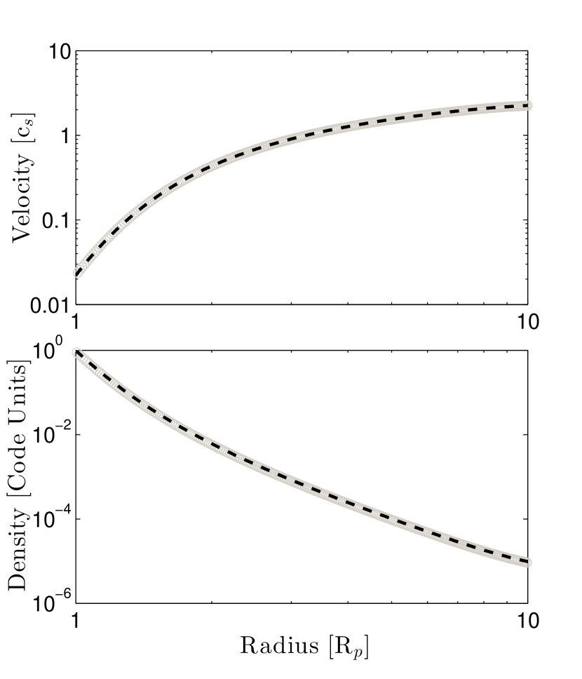
Figure 14: Comparison of the flow profiles obtained from our simulations (grey points) and analtyic solution (dashed line). The relative error between the two curves is approximately 0.003.

References

- Adams (2011) Adams F. C., 2011, ApJ, 730, 27
- Adams & Gregory (2012) Adams F. C., Gregory S. G., 2012, ApJ, 744, 55
- Baraffe et al. (2006) Baraffe I., Alibert Y.. Chabrier G., Benz W., 2006, A&A, 450, 1221
- Batygin & Stevenson (2010) Batygin, K., & Stevenson, D. J. 2010, ApJL, 714, L238
- Batygin et al. (2011) Batygin, K., Stevenson, D. J., & Bodenheimer, P. H. 2011, ApJ, 738, 1
- Bisikalo et al. (2013) Bisikalo, D., Kaygorodov, P., Ionov, D., et al. 2013, ApJ, 764, 19
- Bisikalo & Shematovich (2015) Bisikalo, D. V., & Shematovich, V. I. 2015, Astronomy Reports, 59, 836
- Cranmer (2004) Cranmer S., 2004, Amer. J. Phys., 72, 1397
- Del Zanna et al. (1998) Del Zanna L., Velli M., Londrillo P., 1998, A&A, 330, 13
- Ehrenreich et al. (2015) Ehrenreich, D., Bourrier, V., Wheatley, P. J., et al. 2015, Nature, 522, 459
- García Muñoz (2007) García Muñoz, A., 2007, Planet. Space Sci., 55, 1426
- Güdel et al. (2003) Güdel M., Audard M., Kashyap V. L., Drake J. J., Guinan, E. F., 2003, ApJ, 582, 423
- Hayes et al. (2006) Hayes J. C., Norman M. L., Fiedler R. A., Bordner J. O., Li P. S., Clark S. E., Ud-Doula A., Mac Low M., 2006, ApJS, 165, 188
- Johns-Krull (2007) Johns-Krull C. M., 2007, ApJ, 664, 975
- Koskinen et al. (2013a) Koskinen, T. T., Harris, M. J., Yelle, R. V., & Lavvas, P. 2013a, Icarus, 226, 1678
- Koskinen et al. (2013b) Koskinen, T. T., Yelle, R. V., Harris, M. J., & Lavvas, P. 2013b, Icarus, 226, 1695
- Lammer at al. (2003) Lammer H., Selsis F., Ribas I., Guinan E. F., Bauer S. J., Weiss W. W., 2003, ApJ, 598, 121
- Laughlin et al. (2011) Laughlin, G., Crismani, M., & Adams, F. C. 2011, ApJL, 729, L7
- Lecavelier des Etangs et al. (2004) Lecavelier des Etangs, A., Vidal-Madjar, A., McConnell, J. C., & Hébrard, G. 2004, A&A, 418, L1
- Lecavelier des Etangs et al. (2010) Lecavelier des Etangs, A. et al., 2010, A&A, 514, 72
- Lecavelier des Etangs et al. (2012) Lecavelier des Etangs, A., Bourrier, V., Wheatley, P. J., et al. 2012, A&A, 543, L4
- Matsakos et al. (2015) Matsakos, T., Uribe, A., Königl, A. 2015, A&A, 578, A6
- Menou (2012) Menou, K. 2012, ApJ, 745, 138
- Murray-Clay, Chiang & Murray (2009) Murray-Clay R. A., Chiang E. I., Murray N., 2009, ApJ, 693, 23
- Owen & Jackson (2012) Owen J. E., Jackson A. P., 2012, MNRAS, 425, 2931
- Owen & Wu (2013) Owen J. E., Wu Y., 2013, ApJ, 775, 105
- Owen & Adams (2014) Owen J. E., Adams F. C., 2014, MNRAS, 444, 3761
- Owen & Alvarez (2015) Owen, J. E., & Alvarez, M. A. 2015, ApJ, in press, arXiv:1504.07170
- Parker (1958) Parker E. N., 1958, Phys. Fluids, 1, 171
- Rein (2012) Rein H., 2012, arXiv:1211.7121
- Shematovich et al. (2014) Shematovich, V. I., Ionov, D. E., & Lammer, H. 2014, A&A, 571, A94
- Shkolnik et al. (2005) Shkolnik E., Walker G. A. H., Bohlender D. A., Gu P.-G., Kürster M., 2005, ApJ, 622, 1075
- Shkolnik et al. (2008) Shkolnik E., Bohlender D. A., Walker G. A. H., Collier Cameron A., 2008, ApJ, 676, 628
- Shu (1992) Shu, F. H. 1992, Gas Dynamics (Mill Valley: Univ. Science Books)
- Stone & Norman (1992) Stone J. M., Norman M. L., 1992, ApJS, 80, 753
- Stone & Proga (2009) Stone J. M., Proga D., 2009, ApJ, 694, 205
- Thompson (1987) Thompson K. W., 1987, J. Comput. Phys., 68, 1
- Theuns & David (1992) Theuns, T., & David, M., 1992, ApJ, 384, 587
- Trammell et al. (2011) Trammell G. B., Arras P., Li Z.-Y., 2011, ApJ, 728, 152
- Trammell et al. (2014) Trammell G. B., Arras P., Li Z.-Y., 2014, ApJ, 788, 161
- Van Leer (1977) Van Leer B., 1977, J. Comput. Phys., 23, 276
- Velli (1994) Velli M., 1995, ApJ, 432, 55
- Vidal-Madjar et al. (2003) Vidal-Madjar A., Lecavelier des Etangs A., Dé˝́sert J.-M., Ballester G. E., Ferlet R., Hébrard G., Mayor, M., 2002, Nature, 422, 143
- VonNeumann & Richtmyer (1950) VonNeumann J., Richtmyer R. D., 1950, J. Appl. Phys., 21, 232
- Watson et al. (1981) Watson A., Donahue T., Walker J., 1981, Icarus, 48, 150
- Yelle (2004) Yelle R. V., 2004, Icarus, 170, 167