Non local quantum state engineering with the Cooper pair splitter
beyond the Coulomb blockade regime

Abstract

A Cooper pair splitter consists of two quantum dots side-coupled to a conventional superconductor. Usually, the quantum dots are assumed to have a large charging energy compared to the superconducting gap, in order to suppress processes other than the coherent splitting of Cooper pairs. In this work, in contrast, we investigate the limit in which the charging energy is smaller than the superconducting gap. This allows us, in particular, to study the effect of a Zeeman field comparable to the charging energy. We find analytically that in this parameter regime the superconductor mediates an inter-dot tunneling term with a spin symmetry determined by the Zeeman field. Together with electrostatically tunable quantum dots, we show that this makes it possible to engineer a spin triplet state shared between the quantum dots. Compared to previous works, we thus extend the capabilities of the Cooper pair splitter to create entangled non local electron pairs.

I Introduction

Entanglement Schrödinger (1935) is arguably one of the most fundamental aspects of quantum mechanics and is an essential resource for emerging quantum technologies. Non local entanglement manifests itself in correlations between spatially separated parts of a quantum system that defy any classical explanation. A natural way to explore this phenomenon is by creating EPR pairs of particles, named after the influential Einstein-Podolsky-Rosen paper Einstein et al. (1935), in order to violate Bell’s inequalities Bell (1964); Aspect et al. (1982); Giustina et al. (2015); Hensen et al. (2015); Shalm et al. . These EPR pairs are the basis for many applications of quantum information theory, such as quantum computation DiVincenzo (1995), quantum teleportation Bouwmeester et al. (1997), and quantum communication Ursin et al. (2007).

The preparation of EPR pairs of photons is well established in the field of quantum optics and has already been applied in quantum teleportation and quantum communication Bouwmeester et al. (1997); Ursin et al. (2007). However, preparing an electronic EPR pair has proved to be rather difficult. Still, a solid state source of electronic EPR pairs is highly desirable. For example, (on-demand) generation of electronic EPR pairs would greatly facilitate the construction of quantum repeaters that are essential ingredients of a future quantum network (quantum internet) Kimble (2008). One promising approach makes use of the natural occurrence of singlet pairs of electrons in the ground state of conventional s-wave superconductors. By coupling such a superconductor to two spatially separated quantum dots (QDs), individual Cooper pairs can split and the two electrons from a pair tunnel to a different QD each. Because this process is coherent the resulting state of the two QDs is a non local entangled singlet EPR pair. This process is dominant if both the superconducting gap $\Delta$ and the Coulomb repulsion of electrons on one QD, characterized by the on-site interaction strength $U>0$, are large compared with the single electron tunneling rate between the superconductor and the QDs. Such devices are usually called Cooper pair splitters (CPSs) and were first proposed in Refs. Choi et al. (2000); Recher et al. (2001); Lesovik et al. (2001) and realized experimentally in Refs. Hofstetter et al. (2009); Herrmann et al. (2010); Das et al. (2012). In these experiments, measurements of the current and current noise flowing out of the QDs have confirmed the spatial separation of the electrons from a Cooper pair. Theoretical analysis of the branching currents and their crossed correlations was done in Chevallier et al. (2011); Rech et al. (2012), and the subgap transport was studied in Eldridge et al. (2010). Only recently, measurements of the Josephson current flowing between superconducting contacts through two parallel QDs have demonstrated that the pairs are indeed entangled Deacon et al. (2015). CPSs can also be used to probe the symmetry of the order parameter in unconventional superconductors Tiwari et al. (2014); Sothmann and Tiwari (2015), as a model system exhibiting unconventional pairing Sothmann et al. (2014), to entangle mechanical resonators Walter et al. (2013), or to engineer Majorana bound states which are not topologically protected Leijnse and Flensberg (2012).

Typical theoretical treatments of the CPS assume an infinite charging energy for each QD, making it energetically impossible for two electrons to occupy the same QD. This is known as the Coulomb blockade approximation and is valid as long as the QDs have a relatively large charging energy compared to other relevant energy scales in the device such as the superconducting gap and the thermal energy. In the present work we explore the opposite regime of a small charging energy compared with the superconducting gap. We show that by leveraging a combination of effects due to Coulomb repulsion, finite Zeeman magnetic field, and electrostatic tuning of the system, it is possible to prepare also non local triplet states with zero spin in the CPS system. This is particularly interesting for solid state quantum information processing, where information is encoded in the spin degree of freedom of electrons trapped in semiconductor QD structures DiVincenzo (1995).

The paper is organized as follows: We begin by summarizing the main results obtained in this paper in Sec. II. In Sec. III we describe the model used in this paper for the CPS system. In Sec. IV we introduce the effective low energy Hamiltonian, obtained for zero temperature and a small charging energy in the QDs compared with the superconducting gap. Sec. V introduces a scheme for the generation of a non local triplet state on the two QDs. In Appendix A, we set up and analytically solve a simplified model that captures the essential physics of the triplet generation and in Appendix B we provide details on the employed Schrieffer-Wolff transformation.

II Summary of the main results

For simplicity, we restrict ourselves to the zero temperature limit and consider the coherent dynamics on time scales that are assumed to be much shorter than the coherence time of the system. Employing a Schrieffer-Wolff transformation Schrieffer and Wolff (1966), we integrate out the degrees of freedom of the superconductor and derive an effective low energy model for the dynamics of the QDs [see Eqs. (9) to (12)].

As expected, but in contrast to the case of infinite charging energy, this effective low energy model contains a term that allows two electrons to tunnel to the same QD. This term competes with the Cooper pair splitting process and thus reduces its efficiency. However, this suppression is of order $\Gamma_{0}/U$, where $\Gamma_{0}$ is the bare Cooper pair splitting rate and can thus be made small by reducing the tunneling strength between the superconductor and the QDs at the cost of increasing the duration of singlet generation $\sim 1/\Gamma_{0}$.

More interestingly, we also find that for finite on-site Coulomb repulsion on the QDs, the superconductor induces an effective inter-dot interaction term. In the presence of an (in-plane) magnetic field that lifts the spin degeneracy via the Zeeman effect by $\Delta_{Z}$, the spin symmetry of this new term can be altered and the part which is anti-symmetric under spin exchange can be made to dominate over the zero-field symmetric part. This effect together with electrostatic tuning of the QD levels can be used to generate with high fidelity a non local triplet state with zero spin on the two QDs. We investigate this triplet generation scheme in detail both numerically and, within a simplified model also analytically. We find that in a regime where $\Gamma_{0}\ll U\ll\Delta_{Z}\ll\Delta$, the triplet fidelity that can be achieved is approximately given by

$$\mathcal{F}_{T}\approx 1-\left(\frac{U}{\Delta_{Z}}\right)^{2}-8\left(\frac{\Gamma_{0}}{U}\right)^{2},$$ (1)

which takes its optimal value $\mathcal{F}_{T}\approx 1-2^{5/2}\Gamma_{0}/\Delta_{Z}$ for $U=2^{3/4}\sqrt{\Gamma_{0}\Delta_{Z}}$. This simple and intuitive fidelity formula can be used for a quick estimate of parameters for a given CPS realization. A more general expression for the fidelity, which relaxes some of the above strong inequality constraints is derived in Appendix A.

III Description of the physical system and model

The system we consider is depicted schematically in Fig. 1. It consists of a conventional BCS superconductor tunnel-coupled to two otherwise isolated QDs. We assume the coupling is local, which is justified in the limit where the superconducting coherence length is much larger than the distance between the two points on the superconductor from which the electrons tunnel onto the QDs Recher et al. (2001); Nigg et al. (2015); Falci et al. (2001). We assume that only one orbital energy level per QD is relevant. This approximation essentially requires sufficiently small QDs with large level spacings. This is typical for QDs from the III-V semiconductors, for which the relevant level would be a state from the heavy-hole band Gywat et al. (2010). States in the light-hole and conduction bands can be safely ignored due to their larger detuning from the chemical potential of the superconductor as compared to the coupling strength. We consider the zero-temperature limit where Bogoliubov quasi-particles are absent in the system. The Coulomb repulsion between two electrons of opposite spins on one QD is accounted for by the on-site energies $U_{L}$ (left QD) and $U_{R}$ (right QD). The chemical potentials $\mu_{L}$ and $\mu_{R}$ of the two QDs can be tuned electrostatically by a gate. Finally we also allow for an (in-plane) magnetic field to be applied to the system. This leads to a Zeeman splitting $\Delta_{Z}$ of the QD levels. The full system is modeled by the Hamiltonian

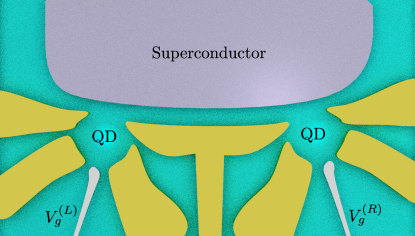
Figure 1: Schematics of the Cooper pair splitter system. Such a system can for example be realized by deposition of a superconductor [wide (purple) structure on the top] on top of a patterned 2DEG at the interface of a semiconductor heterostructure. The 2DEG is electrostatically depleted underneath the superconductor and underneath the gates defining the quantum dots (yellow structures). Further gates (elongated thin gray structures) can be used to electrostatically control the potential of the quantum dots.

$$H=H_{\rm{BCS}}+H_{\rm QDs}+K,$$ (2)

where

$$H_{\rm{BCS}}=\sum_{\sigma}\sum_{k}E_{k}\alpha^{\dagger}_{k\sigma}\alpha_{k\sigma},$$ (3)

describes the BCS superconductor via the Bogoliubov quasi-particle operators $\alpha_{k\sigma}$ and energies $E_{k}$. The Hamiltonians of the QDs are given by

$$H_{\rm QDs}=\sum_{\lambda\in\{L,R\}}\sum_{\sigma\in\{+,-\}}\epsilon_{\lambda\sigma}c^{\dagger}_{\lambda\sigma}c_{\lambda\sigma}+\sum_{\lambda\in\{L,R\}}U_{\lambda}n_{\lambda+}n_{\lambda-}.$$ (4)

Here $c_{\lambda\sigma}$ is a fermionic annihilation operator for an electron with spin $\sigma$ in QD $\lambda$. The corresponding number operator is denoted by $n_{\lambda\sigma}=c_{\lambda\sigma}^{\dagger}c_{\lambda\sigma}$ and the energy levels are given by

$$\epsilon_{\lambda\sigma}=\mu_{\lambda}+\sigma\Delta_{Z}/2.$$ (5)

Finally, the coupling between the QDs and the superconductor is given by the tunneling Hamiltonian

$$K=\sum_{\lambda}w_{\lambda}\sum_{k\sigma}\left(c_{\lambda\sigma}d^{\dagger}_{k\sigma}+{\rm h.c.}\right),$$ (6)

where the tunnel matrix elements $w_{\lambda}$ are assumed to be spin and momentum independent and $d_{k\sigma}$ represents the fermionic annihilation operator for an electron with energy $\xi_{k}$ in the superconductor. In this tunneling Hamiltonian the superconductor is coupled only to the relevant orbital energy level of the QDs (as previously explained).

The electron operators are related to the Bogoliubov operators in the usual fashion:

$$d_{k+} =u_{k}\alpha_{k,+}+v_{k}\alpha^{\dagger}_{-k,-},$$ (7)

$$d_{-k,-} =u_{k}\alpha_{-k,-}-v_{k}\alpha^{\dagger}_{k,+},$$ (8)

with $u_{k}=(1/\sqrt{2})\sqrt{1+\xi_{k}/E_{k}}$, $v_{k}=(1/\sqrt{2})\sqrt{1-\xi_{k}/E_{k}}$ and $E_{k}=\sqrt{\Delta^{2}+\xi_{k}^{2}}$.

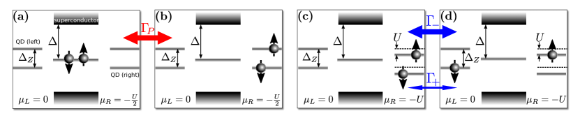
Figure 2: Schematics of the dominant processes for generating the non local triplet state $\ket{T}=(\ket{+}_{L}\ket{-}_{R}+\ket{-}_{L}\ket{+}_{R})/\sqrt{2}$. Panel (a) shows the initial state right after switching the potential of the right QD to $\mu_{R}=-U/2$. Both QDs are unoccupied and electrons form CPs in the superconductor. A magnetic field lifts the spin-degeneracy of the QD levels by $\Delta_{Z}$. Panel (b) shows the state where a CP has been transferred to the right QD at time $T_{1}$. The rate for this process is given by $\Gamma_{P}$, Eq. (IV). Panel (c) shows the state right after time $T_{1}$ when the potential of the right QD has been switched to $-U$. Taking into account the chemical potential and the charging energy, we see that now the energy levels are shifted by $-U$. Panel (d) shows the state after an electron from the right QD (here the down spin electron) has been transferred to the left QD at time $T_{1}+T_{2}$. This process is driven by the inter-dot tunneling term. If $U\ll\Delta_{Z}/2$, the latter is dominated by the spin anti-symmetric term with rate $\Gamma_{-}$, Eq. (16), as compared with the spin symmetric term with rate $\Gamma_{+}$, Eq. (15). The same processes but with the spin states interchanged are equally likely and their amplitudes add coherently resulting in the generation of a triplet state. 

IV Effective low energy model

Since we are interested in a system where the tunnel coupling between the QDs and the superconductor is small compared with both the superconducting gap and the on-site charging energy of the QDs, we proceed in this section to derive an effective low energy Hamiltonian. This model will form the basis of our investigation of the CPS beyond the Coulomb blockade regime.

The first order process described by the tunneling Hamiltonian $K$, is basically the tunneling of a quasi-particle from the superconductor to one of the QDs or the conjugate process. However, as we are working in the limit of zero temperature, quasi-particles are not present. It is therefore useful to distinguish between the “high-energy subspace”, which contains quasi-particle excitations, from the “low-energy subspace”, which contains states with no quasi-particles. Transitions between states in the low-energy subspace can occur via virtual excursions to the high-energy subspace. This picture suggests the use of the Schrieffer-Wolff (SW) transformation Schrieffer and Wolff (1966). The SW transformation eliminates the first order tunneling term from the Hamiltonian, at the expense of introducing all higher orders. By keeping only the leading order terms (second order in $w_{\lambda}$), one obtains an effective low energy Hamiltonian. This procedure effectively integrates out the degrees of freedom of the superconductor and allows for a clearer understanding of the CPS dynamics. The details of this transformation can be found in Appendix B. In order to keep the following expressions more compact, we consider a left-right symmetric system, i.e. $w_{L}=w_{R}=w$ and $U_{L}=U_{R}=U$. The generalization to asymmetric systems is given in Appendix B. Note that the chemical potentials of the left and right QDs can still differ from each other. The resulting effective low energy Hamiltonian is given by

$$H_{\text{LE}}=H_{\text{QDs}}+H_{S}+H_{P}+H_{D},$$ (9)

where $H_{\rm QDs}$ is given in Eq. (4), and the other terms are given by

$$H_{S}=\frac{\Gamma_{0}}{2} \left\{\left(\frac{1}{\sqrt{1-\left(\frac{\Delta_{Z}}{2\Delta}\right)^{2}}}(2-n_{L-}-n_{R+})+\frac{1}{\sqrt{1-\left(\frac{U+\Delta_{Z}/2}{\Delta}\right)^{2}}}n_{L-}+\frac{1}{\sqrt{1-\left(\frac{U-\Delta_{Z}/2}{\Delta}\right)^{2}}}n_{R+}\right)c_{L+}^{\dagger}c_{R-}^{\dagger}\right.$$

$$\left.-\left(\frac{1}{\sqrt{1-\left(\frac{\Delta_{Z}}{2\Delta}\right)^{2}}}(2-n_{L+}-n_{R-})+\frac{1}{\sqrt{1-\left(\frac{U-\Delta_{Z}/2}{\Delta}\right)^{2}}}n_{L+}+\frac{1}{\sqrt{1-\left(\frac{U+\Delta_{Z}/2}{\Delta}\right)^{2}}}n_{R-}\right)c_{L-}^{\dagger}c_{R+}^{\dagger}\right\}+{\rm h.c.}$$ (10)

$$H_{P}=\Gamma_{P} \left(c_{R+}^{\dagger}c_{R-}^{\dagger}+c_{L+}^{\dagger}c_{L-}^{\dagger}\right)+{\rm h.c.}$$ (11)

$$H_{D}=\frac{\Gamma_{0}}{2} \left\{\left(\frac{1}{\sqrt{\left(\frac{\Delta}{U+\Delta_{Z}/2}\right)^{2}-1}}\left(n_{L-}+n_{R-}\right)+\frac{1}{\sqrt{\left(\frac{2\Delta}{\Delta_{Z}}\right)^{2}-1}}\left(2-n_{L-}-n_{R-}\right)\right)c_{L+}c^{\dagger}_{R+}\right.$$

$$+\left.\left(\frac{{\rm sgn}(U-\Delta_{Z}/2)}{\sqrt{\left(\frac{\Delta}{U-\Delta_{Z}/2}\right)^{2}-1}}(n_{L+}+n_{R+})-\frac{1}{\sqrt{\left(\frac{2\Delta}{\Delta_{Z}}\right)^{2}-1}}(2-n_{L+}-n_{R+})\right)c_{L-}c_{R-}^{\dagger}\right\}+{\rm h.c..}$$ (12)

Here we have defined the bare resonant Cooper pair splitting rate $\Gamma_{0}=\pi\rho_{0}|w|^{2}$, where $\rho_{0}$ is the normal state density of states at the Fermi energy of the superconductor, and

$$\Gamma_{P}= \frac{\Gamma_{0}}{2}\left\{\frac{1}{\sqrt{1-\left(\frac{\Delta_{Z}}{2\Delta}\right)^{2}}}+\frac{1/2+\frac{1}{\pi}\tan^{-1}\left(\frac{U+\Delta_{Z}/2}{\sqrt{\Delta^{2}-\left(U+\Delta_{Z}/2\right)^{2}}}\right)}{\sqrt{1-\left(\frac{U+\Delta_{Z}/2}{\Delta}\right)^{2}}}\right.$$

$$\left.+\frac{1/2+\frac{1}{\pi}\tan^{-1}\left(\frac{U-\Delta_{Z}/2}{\sqrt{\Delta^{2}-\left(U-\Delta_{Z}/2\right)^{2}}}\right)}{\sqrt{1-\left(\frac{U-\Delta_{Z}/2}{\Delta}\right)^{2}}}\right\}$$ (13)

is the pair tunneling rate. Each of the above terms describes a different physical process: $H_{S}$ describes the Cooper pair splitting, which now depends on the occupancies of the QDs via the number operators $n_{\lambda\sigma}$. $H_{P}$ describes the pair-tunneling to the same QD. In addition, the superconductor is found to mediate an effective interaction between the two QDs as described by $H_{D}$. The latter term has been derived previously in the infinite $U$ limit Nigg et al. (2015). However, since double occupancy is strictly forbidden, this term does not contribute to the dynamics in the latter case. As we show next, for finite $U$, this term is relevant and can be utilized to generate a non local triplet state on the two QDs. Equations (9) to (12) represent the main technical result of this paper. This effective model is a valid low energy approximation as long as $\Gamma_{0},\Delta_{Z}/2,U\ll\Delta$. In the limit of $\Delta\rightarrow\infty$, this Hamiltonian agrees with previously known results Sothmann et al. (2014), as shown explicitly in Appendix B.

V Triplet generation for finite on-site repulsion and Zeeman field

In this section we present a scheme to generate a non local triplet state on the two QDs with finite on-site repulsion and in the presence of a finite Zeeman field. This scheme is illustrated in Fig. 2. The central ingredient of this scheme is the inter-dot tunneling term $H_{D}$ in the regime where $U<\Delta_{Z}/2$. In this case, when $H_{D}$ acts on a state where one of the QDs is empty while the other is doubly occupied it can be simplified to

$$H_{D}=\Gamma_{+}\left(c_{L+}c_{R+}^{\dagger}+c_{L-}c_{R-}^{\dagger}\right)+\Gamma_{-}\left(c_{L+}c_{R+}^{\dagger}-c_{L-}c_{R-}^{\dagger}\right)+{\rm h.c.},$$ (14)

with

$$\Gamma_{+} =\frac{\Gamma_{0}}{4}\left(\frac{1}{\sqrt{\left(\frac{\Delta}{U+\Delta_{Z}/2}\right)^{2}-1}}-\frac{1}{\sqrt{\left(\frac{\Delta}{U-\Delta_{Z}/2}\right)^{2}-1}}\right)$$ (15)

$$\Gamma_{-} =\frac{\Gamma_{0}}{4}\left(\frac{1}{\sqrt{\left(\frac{\Delta}{U+\Delta_{Z}/2}\right)^{2}-1}}+\frac{1}{\sqrt{\left(\frac{\Delta}{U-\Delta_{Z}/2}\right)^{2}-1}}\right)+\left(\frac{\Delta_{Z}}{2\Delta}\right)\frac{\Gamma_{S}}{2}$$ (16)

$$\Gamma_{S} =\frac{\Gamma_{0}}{\sqrt{1-\left(\frac{\Delta_{Z}}{2\Delta}\right)^{2}}}.$$ (17)

The terms proportional to $\Gamma_{+}$ are symmetric under spin exchange and induce non local singlet pairs while the terms proportional to $\Gamma_{-}$ are anti-symmetric under spin exchange and induce non local triplet pairs. An estimate for the triplet fidelity, given an initially doubly occupied QD, is derived in Appendix A and is given by

$$\mathcal{F}_{T}^{\rm ideal}\approx\frac{1}{1+\left(\frac{\Gamma_{+}}{\Gamma_{-}}\right)^{2}}\approx 1-\left(\frac{U}{\Delta_{Z}}\right)^{2}.$$ (18)

where the last approximation holds if $U\ll\Delta_{Z}\ll\Delta$.

In order to prepare a state where one QD is empty and the other is doubly occupied, we take advantage of the Coulomb repulsion and the gate tunability of the energy levels of the QDs. Specifically, if the charging energy is such that $U/2\gg\Gamma_{0}$ and if we initially detune say the right QD by $\mu_{R}=-U/2$, then the Cooper pair splitting term $H_{S}$ and the inter-dot tunneling term $H_{D}$ are detuned off resonance and hence suppressed while the pair tunneling term to the right QD in $H_{P}=\Gamma_{P}\left(c_{R+}^{\dagger}c_{R-}^{\dagger}+c_{L+}^{\dagger}c_{L-}^{\dagger}\right)$ is made resonant [see Fig. 2, panels (a) and (b)]. Hence after half a Rabi period $T_{1}\approx\frac{\pi}{2}\left(\Gamma_{P}+\frac{4\Gamma_{S}\Gamma_{+}}{U}\right)^{-1}$ the right QD will be doubly occupied and the left QD will be empty. Note that $\Gamma_{S}$ is the CPS rate in a finite Zeeman field. Spurious contributions from off-resonant terms will limit the maximal achievable double occupancy to roughly

$$\mathcal{F}_{D}\approx 1-8\left(\frac{\Gamma_{S}}{U}\right)^{2}.$$ (19)

The derivation of Eq. (19) and of the approximate expression for $T_{1}$ are given in Appendix A.

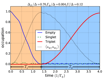
Figure 3: Dynamics of the triplet state generation for $U/\Delta=0.12$, $\Delta_{Z}/\Delta=0.76$ and $\Gamma_{0}/\Delta=0.004$. The two shaded areas of the graph correspond to the two stages of the protocol described in the text and are separated by the switching of the potential of the right QD from $-U/2$ to $-U$, (see also Fig. 2). In the first stage, population is transferred from the vacuum (solid (blue) line) to the doubly occupied state of the right QD (dotted (black) line). In the second stage, population is transferred from the doubly occupied state to the non local triplet (solid thick (red) line). A maximal triplet fidelity of $97\%$ is reached at time $T_{1}+T_{2}$. Note also the presence of a small oscillatory population of the non local singlet state (dashed (green) line).

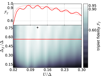
Figure 4: The contour plot shows the fidelity of the triplet state generation as a function of on-site interaction strength $U$ and Zeeman field $\Delta_{Z}$ for $\Gamma_{0}/\Delta=0.004$. The (black) cross indicates the parameters used in the plot of Fig. 3. The solid (red) line in the upper panel shows the fidelity for a fixed value of $\Delta_{Z}=0.56$ indicated by the solid (red) line in the contour plot. In the regime where $\Gamma_{0}\ll U\ll\Delta_{Z}\ll\Delta$, the triplet fidelity is well approximated by the analytic expression $\mathcal{F}_{T}\approx 1-(U/\Delta_{Z})^{2}-8(\Gamma_{0}/U)^{2}$ (dotted (red) line). Weak oscillations of the fidelity as a function of $U$ are clearly visible.

At time $T_{1}$, the right QD is then quickly detuned further to $\mu_{R}=-U$. This detunes the pair tunneling term off resonance and hence suppress it while making the inter-dot term resonant [see Fig. 2, panels (c) and (d)]. After another half Rabi period of $T_{2}\approx(\pi/2)\left[2\left(\Gamma_{-}^{2}+\Gamma_{+}^{2}\right)\right]^{-1/2}$, a state with a large non local triplet population is generated on the two QDs. An estimate for the achievable triplet fidelity in the regime $\Gamma_{0}\ll U\ll\Delta_{Z}\ll\Delta$ is given by

$$\mathcal{F}_{T}\approx\mathcal{F}_{D}\mathcal{F}_{T}^{\rm ideal}\approx 1-\left(\frac{U}{\Delta_{Z}}\right)^{2}-8\left(\frac{\Gamma_{0}}{U}\right)^{2}.$$ (20)

The expression on the right hand side has a simple interpretation: The term $8(\Gamma_{0}/U)^{2}$ describes the loss of fidelity due to the competition between resonant pair tunneling and off resonant Cooper pair splitting in the first stage of the scheme. The term $(U/\Delta_{Z})^{2}$ describes the loss of fidelity during the second stage of the scheme due to the residual spin-symmetric term in $H_{D}$ that favors singlet pairing and competes with the spin anti-symmetric term that favors triplet pairing. A more general analytic expression for the triplet fidelity, which relaxes some of the strong inequality constraints above, is provided in Appendix A.

To confirm the above picture we have numerically solved the Schrödinger equation with the full Hamiltonian (9). The results are illustrated in Fig. 3, where it is shown that a triplet state with $97\%$ fidelity can be obtained for parameters satisfying $\Gamma_{0}\ll U\ll\Delta_{Z}\ll\Delta$.

In the simulation, we assume a chemical potential switching time fast compared to $T_{1}$ and $T_{2}$.

Figure 4 shows how the maximal triplet fidelity depends on the on-site interaction strength and Zeeman field. The general trend is well captured by the analytic approximation (1) (See upper panel of Fig. 4 for a direct comparison). It is noteworthy that for small values of $U$, the fidelity suppression is somewhat stronger than predicted by Eq. (1). This together with the weak oscillations of the fidelity as a function of $U$ can be attributed to higher order terms, neglected in the analytic approximation.

In order to experimentally verify the successful generation of a non local triplet and distinguishing it from a non local singlet state, we propose two different schemes. Firstly, the QDs could be attached to mesoscopic wires forming the inputs of an electronic beam-splitter. Depending on whether the two interfering electrons form a singlet or a triplet, the sign of the two particle interference term will differ Burkard et al. (2000); Samuelsson et al. (2004). Secondly, a gate tunable direct inter-dot tunneling term makes it possible to employ the spin-blockade technique pioneered in Ono et al. (2002); Petta et al. (2005). This enables a mapping from the two spin states onto two distinct charge states of one of the two QDs. The charge states can then be distinguished via a capacitively coupled rf-single electron transistor device Schoelkopf et al. (1998); Goldhaber-Gordon et al. (1998).

VI Conclusions

In conclusion, our work represents a first step in the investigation of the CPS beyond the infinite $U$ limit. We analyze effects of electron-electron interaction in the CPS in the presence or absence of a magnetic Zeeman field. We derive an analytic low energy effective Hamiltonian for this system and identify a novel term that describes an inter-QD interaction mediated by the superconductor. We make use of this interaction and of the electrostatic tunability of the QD levels, to propose a scheme to generate a non local triplet state on the two QDs. Thereby we extend the capabilities of the CPS to generate two of the four maximally entangled Bell states with high fidelities. Experimental investigations testing the validity of the presented effective low energy model in this novel parameter regime seem feasible with current technologies and would be a very useful step towards quantum state engineering with the CPS.

Appendix A Analytic model of triplet state generation

In this appendix, we introduce and analytically solve a simplified model for the dynamics of the triplet state generation presented in Section V. We motivate this model using Fig. 3, which shows the population dynamics in the parameter regime suitable for triplet generation. The crucial observation is that in each of the two stages of the drive scheme, only three states are significantly populated. More specifically, in stage I, these states are (i) the vacuum $\ket{V}=\ket{0}_{L}\ket{0}_{R}$, (ii) the doubly occupied state of the right QD $\ket{D}=c_{R+}^{\dagger}c_{R-}^{\dagger}\ket{V}$ and (iii) the non local singlet state $\ket{S}=(c_{L+}^{\dagger}c_{R-}^{\dagger}-c_{L-}^{\dagger}c_{R+}^{\dagger})/\sqrt{2}\ket{V}$. In stage II the three states are (i) the doubly occupied state $\ket{D}$, (ii) the non local triplet state $\ket{T}=(c_{L+}^{\dagger}c_{R-}^{\dagger}+c_{L-}^{\dagger}c_{R+}^{\dagger})/\sqrt{2}\ket{V}$ and (iii) the non local singlet $\ket{S}$. This fact suggests that we can approximately neglect the occupation of all other states and project the system onto three dimensional subspaces in both stages I and II and match the solutions at the interface (i.e. at time $T_{1}$). We proceed by treating the two stages separately.

Stage I: In the subspace$\{\ket{V},\ket{D},\ket{S}\}$ the Hamiltonian is given by

$$H_{\rm I}=\begin{pmatrix}0&\Gamma_{\text{P}}&\sqrt{2}\Gamma_{\text{S}}\\ \Gamma_{\text{P}}&0&\sqrt{2}\Gamma_{+}\\ \sqrt{2}\Gamma_{\text{S}}&\sqrt{2}\Gamma_{+}&-U/2\\ \end{pmatrix},$$ (21)

where the matrix elements are defined in terms of the rates given in the main text (See Eqs. (11), (15) and (17)) and the factors of $\sqrt{2}$ appear because of the normalization of the singlet state. We now make use of the fact that in stage I, the QDs are tuned such that the vacuum state and the doubly occupied state are resonant with each other while the singlet is off resonance by $U/2\gg\Gamma_{S},\Gamma_{+},\Gamma_{P}$. To carry out the degenerate perturbation theory, we switch to a new basis given by the states

$$\ket{0} \equiv\frac{1}{\sqrt{2}}\left(\ket{V}+\ket{D}\right)$$ (22)

$$\ket{1} \equiv\frac{1}{\sqrt{2}}\left(\ket{V}-\ket{D}\right)$$ (23)

$$\ket{2} \equiv\ket{S}.$$ (24)

In this new basis, the Hamiltonian takes the form

$$H=\begin{pmatrix}\Gamma_{\text{P}}&0&\Gamma_{\text{S}}+\Gamma_{\text{+}}\\ 0&-\Gamma_{\text{P}}&\Gamma_{\text{S}}-\Gamma_{\text{+}}\\ \Gamma_{\text{S}}+\Gamma_{\text{+}}&\Gamma_{\text{S}}-\Gamma_{\text{+}}&-U/2\\ \end{pmatrix}.$$ (25)

Treating the off-diagonal terms as perturbation, we find the corrections to the states $\ket{0},\ket{1}$ and $\ket{2}$ and the corresponding eigenenergies up to second order:

$$\ket{\tilde{0}} =\frac{\ket{V}+\ket{D}}{\sqrt{2}}+\frac{\Gamma_{\text{S}}+\Gamma_{\text{+}}}{U/2+\Gamma_{\text{P}}}\ket{S},$$ (26)

$$\ket{\tilde{1}} =\frac{\ket{V}-\ket{D}}{\sqrt{2}}+\frac{\Gamma_{\text{S}}-\Gamma_{\text{+}}}{U/2-\Gamma_{\text{P}}}\ket{S},$$ (27)

$$\ket{\tilde{2}} =\ket{S}$$ (28)

$$+\sqrt{2}\left(\frac{\Gamma_{\text{S}}U/2-\Gamma_{\text{+}}\Gamma_{\text{P}}}{\Gamma_{\text{P}}^{2}-(U/2)^{2}}\ket{V}+\frac{\Gamma_{\text{+}}U/2-\Gamma_{\text{S}}\Gamma_{\text{P}}}{\Gamma_{\text{P}}^{2}-(U/2)^{2}}\ket{D}\right)$$

$$\tilde{E}_{0} =\Gamma_{\text{P}}+\frac{(\Gamma_{\text{S}}+\Gamma_{\text{+}})^{2}}{U/2+\Gamma_{\text{P}}},$$ (29)

$$\tilde{E}_{1} =-\Gamma_{\text{P}}+\frac{(\Gamma_{\text{S}}-\Gamma_{\text{+}})^{2}}{U/2-\Gamma_{\text{P}}},$$ (30)

$$\tilde{E}_{2} =-\frac{U}{2}-\frac{(\Gamma_{\text{S}}+\Gamma_{\text{+}})^{2}}{U/2+\Gamma_{\text{P}}}-\frac{(\Gamma_{\text{S}}-\Gamma_{\text{+}})^{2}}{U/2-\Gamma_{\text{P}}}.$$ (31)

Assuming that at time $t=0$ the system is in the vacuum state $\ket{V}$, we can approximate the state at time $t$ as

$$\ket{\psi(t)}=\sum_{n=0}^{2}e^{-i\tilde{E}_{n}t/\hbar}\braket{\tilde{n}}{V}\ket{\tilde{n}}.$$ (32)

Hence the probability that the right QD is doubly occupied at time $t$ (equivalent to the fidelity of the doubly occupied state) is found to be

$$\mathcal{F}^{({\rm I})}_{D}(t)=|\braket{D}{\psi(t)}|^{2}=\frac{1}{1+\frac{8\Gamma_{\text{S}}^{2}}{U^{2}}}\left\{\sin^{2}\left[t\left(\Gamma_{\text{P}}+\frac{4\Gamma_{\text{S}}\Gamma_{\text{+}}}{U}\right)\right]\right.\\ \left.-\frac{16\Gamma_{\text{S}}\Gamma_{\text{+}}}{U^{2}}\sin\left(\Gamma_{\text{P}}t\right)\sin\left[t\left(\frac{U}{2}+6\frac{\Gamma_{\text{S}}^{2}+\Gamma_{\text{+}}^{2}}{U}\right)\right]\right\}.$$ (33)

The term on the first line of this equation described the leading order suppression of the fidelity due to the off-resonant transitions between the vacuum and the singlet while the second line describes higher order corrections ($\sim\mathcal{O}\left(\Gamma_{S}\Gamma_{+}/U^{2}\right)$). Physically the latter describe the second order process where a non local singlet is first created out of the vacuum and then transferred to a doubly occupied state by the action of the spin-symmetric part of the inter-dot tunneling Hamiltonian. Because the amplitude of this process adds coherently, it leads to small amplitude oscillations of the fidelity at a frequency of the order of charging energy $U$. Neglecting these small oscillations and expanding to leading order, we obtain the estimates for the optimal double occupancy time $T_{1}\approx\frac{\pi}{2}\left(\Gamma_{P}+\frac{4\Gamma_{S}\Gamma_{+}}{U}\right)^{-1}$ as well as the maximal fidelity of double occupancy $\mathcal{F}_{D}\approx 1-8(\Gamma_{S}/U)^{2}$ given in Eq. (19). Using the perturbative approach, we note also that the probability for the system to be found in the vacuum state $\ket{V}$ at time $t$ is

$$\mathcal{F}^{({\rm I})}_{V}(t)=\frac{1}{1+\frac{8\Gamma_{\text{S}}^{2}}{U^{2}}}\left\{\cos^{2}\left[t\left(\Gamma_{\text{P}}+\frac{4\Gamma_{\text{S}}\Gamma_{+}}{U}\right)\right]\right.\\ \left.+\frac{16\Gamma_{\text{S}}^{2}}{U^{2}}\cos\left(\Gamma_{\text{P}}t\right)\cos\left[t\left(\frac{U}{2}+6\frac{\Gamma_{\text{S}}^{2}+\Gamma_{+}^{2}}{U}\right)\right]\right\},$$ (34)

and the the probability for the system to be found in the singlet state $\ket{S}$ at time $t$ is given by

$$\mathcal{F}^{({\rm I})}_{S}(t)=\frac{2}{U^{2}+8\Gamma_{\text{S}}^{2}}\left\{4\Gamma_{S}^{2}+\Gamma_{\text{S}}^{2}\sin^{2}\left[t\left(\Gamma_{\text{P}}+\frac{4\Gamma_{\text{S}}\Gamma_{+}}{U}\right)\right]\right.$$ (35)

$$\left.\qquad\qquad\qquad+4\Gamma_{\text{S}}^{2}\left(\cos^{2}\left[t\left(\Gamma_{\text{P}}+\frac{4\Gamma_{\text{S}}\Gamma_{+}}{U}\right)\right]\right.\right.$$

$$\left.\left.\qquad\qquad\qquad\qquad-2\cos\left(\Gamma_{\text{P}}t\right)\cos\left[t\left(\frac{U}{2}+6\frac{\Gamma_{\text{S}}^{2}+\Gamma_{+}^{2}}{U}\right)\right]\right)\right\}$$

Stage II: The analysis of stage II is very similar. In this stage the relevant states form the subspace $\{\ket{D},\ket{T},\ket{S}\}$. The resulting three level Hamiltonian is given by

$$H=\begin{pmatrix}-U&\sqrt{2}\Gamma_{-}&\sqrt{2}\Gamma_{+}\\ \sqrt{2}\Gamma_{-}&-U&0\\ \sqrt{2}\Gamma_{+}&0&-U\\ \end{pmatrix},$$ (36)

where $\Gamma_{-}$ was defined in Eq. (16). Owing to the threefold degeneracy of the bare states, this Hamiltonian can easily be diagonalized. The eigenstates are given by

$$\ket{\psi_{0}}=\frac{1}{\sqrt{\Gamma_{\text{+}}^{2}+\Gamma_{-}^{2}}}\left(-\Gamma_{+}\ket{T}+\Gamma_{-}\ket{S}\right),$$ (37)

$$\ket{\psi_{1}}=\frac{1}{\sqrt{2\left(\Gamma_{\text{+}}^{2}+\Gamma_{-}^{2}\right)}}\left(-\sqrt{\Gamma_{+}^{2}+\Gamma_{-}^{2}}\ket{D}+\Gamma_{-}\ket{T}+\Gamma_{\text{+}}\ket{S}\right),$$ (38)

$$\ket{\psi_{2}}=\frac{1}{\sqrt{2\left(\Gamma_{\text{+}}^{2}+\Gamma_{-}^{2}\right)}}\left(\sqrt{\Gamma_{+}^{2}+\Gamma_{-}^{2}}\ket{D}+\Gamma_{-}\ket{T}+\Gamma_{+}\ket{S}\right).$$ (39)

The corresponding eigenenergies are

$$E_{0} =-U,$$ (40)

$$E_{1} =-U-\sqrt{2\left(\Gamma_{\text{+}}^{2}+\Gamma_{-}^{2}\right)},$$ (41)

$$E_{2} =-U+\sqrt{2\left(\Gamma_{\text{+}}^{2}+\Gamma_{-}^{2}\right)}.$$ (42)

To account for an imperfect state preparation after stage I, we consider and initial state for stage II of the form $a\ket{D}+b\ket{S}$ with $|a|^{2}+|b|^{2}=1$. With this, the probability of finding the system in the triplet state $\ket{T}$ at time $t$ is given by

$$\mathcal{F}^{({\rm II})}_{T}(t)=\frac{\Gamma_{-}^{2}}{\left(\Gamma_{+}^{2}+\Gamma_{-}^{2}\right)^{2}}\times\left\{|a|^{2}\left(\Gamma_{+}^{2}+\Gamma_{-}^{2}\right)\sin^{2}\left(t\sqrt{2\left(\Gamma_{+}^{2}+\Gamma_{-}^{2}\right)}\right)\right.\\ \left.+|b|^{2}\Gamma_{+}^{2}\left[1-2\cos\left(t\sqrt{2\left(\Gamma_{+}^{2}+\Gamma_{-}^{2}\right)}\right)+\cos^{2}\left(t\sqrt{2\left(\Gamma_{+}^{2}+\Gamma_{-}^{2}\right)}\right)\right]\right\}.$$ (43)

Note that because only the initial state probabilities $|a|^{2}$ and $|b|^{2}$ appear in Eq. (43), there are no interference terms between stage I and II in the present approach. Thus we can simply obtain the triplet fidelity by multiplying the fidelities of the double occupancy (33) and the ideal triplet fidelity obtained from (43) by setting $a=1$ and $b=0$. The latter is given by

$$\mathcal{F}_{T}^{\rm ideal}(t)=\frac{1}{1+\left(\frac{\Gamma_{+}}{\Gamma_{-}}\right)^{2}}\sin^{2}\left(t\sqrt{2\left(\Gamma_{+}^{2}+\Gamma_{-}^{2}\right)}\right),$$ (44)

from which we immediately obtain an estimate for the ideal duration of stage II: $T_{2}\approx(\pi/2)\left[2\left(\Gamma_{-}^{2}+\Gamma_{+}^{2}\right)\right]^{-1/2}$. Combining these expressions and expanding to leading order in the regime where $\Gamma_{0}\ll U\ll\Delta_{Z}\ll\Delta$, we obtain the expression for the triplet fidelity of Eq. (1).

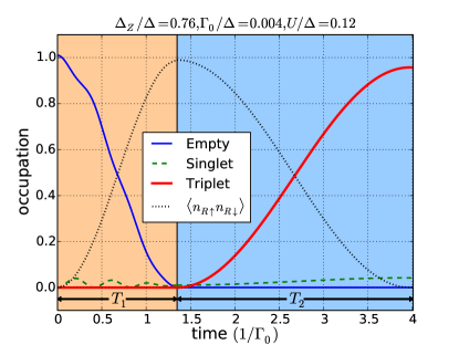
Figure 5: Analytical prediction for the dynamics of the triplet state generation for $U/\Delta=0.12$, $\Delta_{Z}/\Delta=0.76$ and $\Gamma_{0}/\Delta=0.004$. This result agrees qualitatively with the full numerics shown in Fig. 3.

Using this analytic model, we also note that the probability for the system to be found in the doubly occupied state $\ket{D}$ at time $t$ is given by

$$\mathcal{F}^{({\rm II})}_{D}(t)=|a|^{2}\cos^{2}\left(t\sqrt{2\left(\Gamma_{+}^{2}+\Gamma_{-}^{2}\right)}\right)\\ +\frac{|b|^{2}}{1+\left(\frac{\Gamma_{-}}{\Gamma_{+}}\right)^{2}}\sin^{2}\left(t\sqrt{2\left(\Gamma_{+}^{2}+\Gamma_{-}^{2}\right)}\right),$$ (45)

while the probability for the system to be found in the singlet state $\ket{S}$ at time $t$ is given by

$$\mathcal{F}^{({\rm II})}_{S}(t)=\frac{\Gamma_{+}^{2}}{\left(\Gamma_{+}^{2}+\Gamma_{-}^{2}\right)^{2}}\times\left\{|a|^{2}\left(\Gamma_{+}^{2}+\Gamma_{-}^{2}\right)\sin^{2}\left(t\sqrt{2\left(\Gamma_{+}^{2}+\Gamma_{-}^{2}\right)}\right)\right.\\ \left.+|b|^{2}\Gamma_{+}^{2}\left[\frac{\Gamma_{-}^{4}}{\Gamma_{+}^{4}}+\frac{2\Gamma_{-}^{2}}{\Gamma_{+}^{2}}\cos\left(t\sqrt{2\left(\Gamma_{+}^{2}+\Gamma_{-}^{2}\right)}\right)+\right.\right.\\ \left.\left.\cos^{2}\left(t\sqrt{2\left(\Gamma_{+}^{2}+\Gamma_{-}^{2}\right)}\right)\right]\right\}.$$ (46)

We have plotted in Fig. 5 the occupation of the different states in stage I and in stage II using the analytical results obtained, Eq. (33-35), Eq. (43) and Eq. (45-46). This can be compared with Fig. 3.

Appendix B The Schrieffer-Wolff transformation with finite on-site repulsion and Zeeman field

In this Appendix, we present the SW transformation we have used in order to eliminate the first order tunneling term appearing in the original Hamiltonian $H$, Eq. (2), thus leading (after neglecting higher than second order terms in the tunneling amplitude) to the effective low energy Hamiltonian $H_{\text{LE}}$, Eq. (9).

The SW transformation Schrieffer and Wolff (1966) is a unitary transformation, $U\equiv e^{S}$. After transforming $H$ we obtain

$$\tilde{H}=H+[S,H]+\frac{1}{2!}\left[S,[S,H]\right]+\ldots+\frac{1}{n!}\left[S\left[S,\left[\ldots[S,H]\ldots\right]\right]\right]+\ldots$$ (47)

We choose the generator $S$ of the canonical transformation such that it eliminates the perturbation to first order in $w_{\lambda}$, i.e.

$$[S,H_{\text{BCS}}+H_{\text{QDs}}]=-K.$$ (48)

Then, the transformed Hamiltonian becomes,

$$\tilde{H}=H_{\text{BCS}}+H_{\text{QDs}}+\frac{1}{2}[S,K]+\mathcal{O}(w_{\lambda}^{3}).$$ (49)

Keeping terms up to second order in $w_{\lambda}/\Delta$, we find our low energy Hamiltonian,

$$H_{\text{LE}}=H_{\text{BCS}}+H_{\text{QDs}}+H_{\text{SW}},$$ (50)

where we have defined $H_{\text{SW}}\equiv[S,K]/2$. The solution of Eq. (48) is given by Salomaa (1988)

$$\begin{split}S=&\sum_{\lambda}\sum_{k}\sum_{\sigma}w_{\lambda k}\left[\left(\frac{1-n_{\lambda\bar{\sigma}}}{E_{k}-\epsilon_{\lambda,\sigma}}+\frac{n_{\lambda\bar{\sigma}}}{E_{k}-\epsilon_{\lambda,\sigma}-U_{\lambda}}\right)u_{k}\alpha_{k\sigma}^{\dagger}c_{\lambda\sigma}\right.\\ &\left.+\sigma\left(\frac{1-n_{\lambda\sigma}}{E_{k}+\epsilon_{\lambda,\bar{\sigma}}}+\frac{n_{\lambda\sigma}}{E_{k}+\epsilon_{\lambda,\bar{\sigma}}+U_{\lambda}}\right)v_{k}\alpha_{k\sigma}c_{\lambda\bar{\sigma}}\right]-{\rm h.c.},\end{split}$$ (51)

as can be easily verified by substitution. Using this generator, one can calculate $H_{\text{SW}}$. This can be done quite generally, for different values of $\Delta,\Delta_{Z},U_{\lambda}$ and $K_{B}T$ (as long as one keeps in mind that keeping the leading order term in the SW transformation is justified for $\Delta\gg K_{B}T$). However, as we are interested in the regime where the superconducting gap $\Delta$ is much larger than the thermal energy, we furthermore assume that the superconductor is at zero temperature (i.e. we eliminate the quasi particle $\alpha_{k\sigma}$ degrees of freedom by taking the expectation value of $H_{\text{SW}}$ in a state with no quasi-particles). After integrating out the $k$ dependence using the assumption $\Delta>U_{\lambda}+\Delta_{Z}/2$, one obtains an effective low energy Hamiltonian,

$$H_{\text{LE}}=H_{\text{QDs}}+H_{S}+H_{P}+H_{D},$$ (52)

where $H_{\text{QDs}}$ is the QDs Hamiltonian appearing in Eq. (4), and the other terms are given by

$$H_{S} =\frac{\pi\rho_{0}w_{L}w_{R}}{2}\left\{\left(\frac{1}{\sqrt{1-\left(\frac{\Delta_{Z}}{2\Delta}\right)^{2}}}(2-n_{L-}-n_{R+})+\frac{1}{\sqrt{1-\left(\frac{\Delta_{Z}/2+U_{L}}{\Delta}\right)^{2}}}n_{L-}+\frac{1}{\sqrt{1-\left(\frac{\Delta_{Z}/2-U_{R}}{\Delta}\right)^{2}}}n_{R+}\right)c_{L+}^{\dagger}c_{R-}^{\dagger}\right.$$

$$\left.-\left(\frac{1}{\sqrt{1-\left(\frac{\Delta_{Z}}{2\Delta}\right)^{2}}}(2-n_{R-}-n_{L+})+\frac{1}{\sqrt{1-\left(\frac{\Delta_{Z}/2-U_{L}}{\Delta}\right)^{2}}}n_{L+}+\frac{1}{\sqrt{1-\left(\frac{\Delta_{Z}/2+U_{R}}{\Delta}\right)^{2}}}n_{R-}\right)c_{L-}^{\dagger}c_{R+}^{\dagger}\right\}+{\rm h.c.},$$ (53)

$$H_{P} =\frac{\pi\rho_{0}}{2}\left\{\left(\frac{1}{\sqrt{1-\left(\frac{\Delta_{Z}}{2\Delta}\right)^{2}}}+\frac{1/2+\frac{1}{\pi}\tan^{-1}\left(\frac{\frac{\Delta_{Z}/2+U_{R}}{\Delta}}{\sqrt{1-\left(\frac{\Delta_{Z}/2+U_{R}}{\Delta}\right)^{2}}}\right)}{\sqrt{1-\left(\frac{\Delta_{Z}/2+U_{R}}{\Delta}\right)^{2}}}+\frac{1/2-\frac{1}{\pi}\tan^{-1}\left(\frac{\frac{\Delta_{Z}/2-U_{R}}{\Delta}}{\sqrt{1-\left(\frac{\Delta_{Z}/2-U_{R}}{\Delta}\right)^{2}}}\right)}{\sqrt{1-\left(\frac{\Delta_{Z}/2-U_{R}}{\Delta}\right)^{2}}}\right)w_{R}^{2}c_{R+}^{\dagger}c_{R-}^{\dagger}\right.$$

$$\left.+\left(\frac{1}{\sqrt{1-\left(\frac{\Delta_{Z}}{2\Delta}\right)^{2}}}+\frac{1/2+\frac{1}{\pi}\tan^{-1}\left(\frac{\frac{\Delta_{Z}/2+U_{L}}{\Delta}}{\sqrt{1-\left(\frac{\Delta_{Z}/2+U_{L}}{\Delta}\right)^{2}}}\right)}{\sqrt{1-\left(\frac{\Delta_{Z}/2+U_{L}}{\Delta}\right)^{2}}}+\frac{1/2-\frac{1}{\pi}\tan^{-1}\left(\frac{\frac{\Delta_{Z}/2-U_{L}}{\Delta}}{\sqrt{1-\left(\frac{\Delta_{Z}/2-U_{L}}{\Delta}\right)^{2}}}\right)}{\sqrt{1-\left(\frac{\Delta_{Z}/2-U_{L}}{\Delta}\right)^{2}}}\right)w_{L}^{2}c_{L+}^{\dagger}c_{L-}^{\dagger}\right\}+{\rm h.c.},$$ (54)

$$H_{D} =\frac{\pi\rho_{0}w_{L}w_{R}}{2}\left\{\left(\frac{1}{\sqrt{\left(\frac{2\Delta}{\Delta_{Z}}\right)^{2}-1}}(2-n_{L-}-n_{R-})+\frac{1}{\sqrt{\left(\frac{\Delta}{\Delta_{Z}/2+U_{L}}\right)^{2}-1}}n_{L-}+\frac{1}{\sqrt{\left(\frac{\Delta}{\Delta_{Z}/2+U_{R}}\right)^{2}-1}}n_{R-}\right)c_{L+}c^{\dagger}_{R+}\right.$$

$$\left.-\left(\frac{1}{\sqrt{\left(\frac{2\Delta}{\Delta_{Z}}\right)^{2}-1}}(2-n_{L+}-n_{R+})+\frac{{\rm sgn}\left(\Delta_{Z}/2-U_{R}\right)}{\sqrt{\left(\frac{\Delta}{\Delta_{Z}/2-U_{R}}\right)^{2}-1}}n_{R+}+\frac{{\rm sgn}\left(\Delta_{Z}/2-U_{L}\right)}{\sqrt{\left(\frac{\Delta}{\Delta_{Z}/2-U_{L}}\right)^{2}-1}}n_{L+}\right)c_{L-}c_{R-}^{\dagger}\right\}+{\rm h.c.},$$ (55)

where $H_{S}$ contains the standard Cooper pair splitting process which, in contrast to the Cooper pair splitting described using the Coulomb blockade approximation, depends now on the occupation of the QDs via the number operators. $H_{p}$ describes the tunneling of a Cooper pair onto a single QD, and $H_{D}$ describes and effective inter-dot tunneling processes which is mediated via the superconductor. The processes described in $H_{P}$ and in $H_{D}$ are obviously not accounted for in the standard Coulomb blockade approximation. Assuming $w_{L}=w_{R}=w$ and $U_{L}=U_{R}=U$, one can obtain the reduced form of the low energy Hamiltonian which is given in the main text, Eq. (9). In the zero field limit these expressions further simplify and are provided here for completeness. They read:

$$H_{S}^{\Delta_{Z}\rightarrow 0}=\frac{\Gamma_{0}}{2}\left\{\left(2-n_{L-}-n_{R+}+\frac{n_{L-}+n_{R+}}{\sqrt{1-\left(\frac{U}{\Delta}\right)^{2}}}\right)c_{L+}^{\dagger}c_{R-}^{\dagger}\right.$$

$$-\left.\left(2-n_{L+}-n_{R-}+\frac{n_{L+}+n_{R-}}{\sqrt{1-\left(\frac{U}{\Delta}\right)^{2}}}\right)c_{L-}^{\dagger}c_{R+}^{\dagger}\right\}+{\rm h.c.}$$ (56)

$$H_{P}^{\Delta_{Z}\rightarrow 0} =\frac{\Gamma_{0}}{2}\left(1+\frac{1+\frac{2}{\pi}\tan^{-1}\left(\frac{1}{\sqrt{\left(\frac{\Delta}{U}\right)^{2}-1}}\right)}{\sqrt{1-\left(\frac{U}{\Delta}\right)^{2}}}\right)\sum_{\alpha=L,R}c_{\alpha+}^{\dagger}c_{\alpha-}^{\dagger}+{\rm h.c.}$$ (57)

and

$$H_{D}^{\Delta_{Z}\rightarrow 0} =\frac{\Gamma_{0}}{2}\frac{1}{\sqrt{\left(\frac{\Delta}{U}\right)^{2}-1}}\sum_{\sigma=\pm}\left(n_{L\sigma}+n_{R\sigma}\right)c_{L\bar{\sigma}}c_{R\bar{\sigma}}^{\dagger}+{\rm h.c.}$$ (58)

Further insight into the effective Hamiltonian in Eq. (52) can be gained by examining the limiting case of an infinite superconducting gap. In that limit, important for transport processes involving Andreev reflection, effective Hamiltonians for proximised QDs have already been introduced in the literature Eldridge et al. (2010); Sothmann et al. (2014); Droste et al. (2012). Taking this limit in Eq. (52), one obtains

$$H_{\text{LE}}^{\Delta\rightarrow\infty}=H_{\text{QDs}}+\pi\rho_{0}\omega_{L}\omega_{R}\left(c_{L+}^{\dagger}c_{R-}^{\dagger}-c_{L-}^{\dagger}c_{R+}^{\dagger}+{\rm h.c.}\right)\\ +\pi\rho_{0}\left(\omega_{R}^{2}c_{R+}^{\dagger}c_{R-}^{\dagger}+\omega_{L}^{2}c_{L+}^{\dagger}c_{L-}^{\dagger}+{\rm h.c.}\right).$$ (59)

This result agrees with Sothmann et al. (2014) for example.

References

• Schrödinger (1935) E. Schrödinger, Math. Proc. Cambridge 31, 555 (1935).
• Einstein et al. (1935) A. Einstein, B. Podolsky, and N. Rosen, Phys. Rev. 47, 777 (1935).
• Bell (1964) J. S. Bell, Physics 1, 195 (1964).
• Aspect et al. (1982) A. Aspect, J. Dalibard, and G. Roger, Phys. Rev. Lett. 49, 1804 (1982).
• Giustina et al. (2015) M. Giustina, M. A. M. Versteegh, S. Wengerowsky, J. Handsteiner, A. Hochrainer, K. Phelan, F. Steinlechner, J. Kofler, J.-A. Larsson, C. Abellán, et al., Phys. Rev. Lett. 115, 250401 (2015).
• Hensen et al. (2015) B. Hensen, H. Bernien, A. E. Dreau, A. Reiserer, N. Kalb, M. S. Blok, J. Ruitenberg, R. F. L. Vermeulen, R. N. Schouten, C. Abellan, et al., Nature 526, 682 (2015).
• (7) L. K. Shalm, E. Meyer-Scott, B. G. Christensen, P. Bierhorst, M. A. Wayne, M. J. Stevens, T. Gerrits, S. Glancy, D. R. Hamel, M. S. Allman, et al., arXiv:1511.03190.
• DiVincenzo (1995) D. P. DiVincenzo, Science 270, 255 (1995).
• Bouwmeester et al. (1997) D. Bouwmeester, J.-W. Pan, K. Mattle, M. Eibl, H. Weinfurter, and A. Zeilinger, Nature 390, 575 (1997).
• Ursin et al. (2007) R. Ursin, F. Tiefenbacher, T. Schmitt-Manderbach, H. Weier, T. Scheidl, M. Lindenthal, B. Blauensteiner, T. Jennewein, J. Perdigues, P. Trojek, et al., Nature Phys. 3, 481 (2007).
• Kimble (2008) H. J. Kimble, Nature 453, 1023 (2008).
• Choi et al. (2000) M.-S. Choi, C. Bruder, and D. Loss, Phys. Rev. B 62, 13569 (2000).
• Recher et al. (2001) P. Recher, E. V. Sukhorukov, and D. Loss, Phys. Rev. B 63, 165314 (2001).
• Lesovik et al. (2001) G. B. Lesovik, T. Martin, and G. Blatter, Eur. Phys. J. B 24, 287 (2001).
• Hofstetter et al. (2009) L. Hofstetter, S. Csonka, J. Nygard, and C. Schönenberger, Nature 461, 960 (2009).
• Herrmann et al. (2010) L. G. Herrmann, F. Portier, P. Roche, A. L. Yeyati, T. Kontos, and C. Strunk, Phys. Rev. Lett. 104, 026801 (2010).
• Das et al. (2012) A. Das, Y. Ronen, M. Heiblum, D. Mahalu, A. V. Kretinin, and H. Shtrikman, Nat. Comm. 3, 1165 (2012).
• Chevallier et al. (2011) D. Chevallier, J. Rech, T. Jonckheere, and T. Martin, Phys. Rev. B 83, 125421 (2011).
• Rech et al. (2012) J. Rech, D. Chevallier, T. Jonckheere, and T. Martin, Phys. Rev. B 85, 035419 (2012).
• Eldridge et al. (2010) J. Eldridge, M. G. Pala, M. Governale, and J. König, Phys. Rev. B 82, 184507 (2010).
• Deacon et al. (2015) R. S. Deacon, A. Oiwa, J. Sailer, S. Baba, Y. Kanai, K. Shibata, K. Hirakawa, and S. Tarucha, Nat. Comm. 6, 7446 (2015).
• Tiwari et al. (2014) R. P. Tiwari, W. Belzig, M. Sigrist, and C. Bruder, Phys. Rev. B 89, 184512 (2014).
• Sothmann and Tiwari (2015) B. Sothmann and R. P. Tiwari, Phys. Rev. B 92, 014504 (2015).
• Sothmann et al. (2014) B. Sothmann, S. Weiss, M. Governale, and J. König, Phys. Rev. B 90, 220501 (2014).
• Walter et al. (2013) S. Walter, J. C. Budich, J. Eisert, and B. Trauzettel, Phys. Rev. B 88, 035441 (2013).
• Leijnse and Flensberg (2012) M. Leijnse and K. Flensberg, Phys. Rev. B 86, 134528 (2012).
• Schrieffer and Wolff (1966) J. R. Schrieffer and P. A. Wolff, Phys. Rev. 149, 491 (1966).
• Nigg et al. (2015) S. E. Nigg, R. P. Tiwari, S. Walter, and T. L. Schmidt, Phys. Rev. B 91, 094516 (2015).
• Falci et al. (2001) G. Falci, D. Feinberg, and F. W. J. Hekking, EPL (Europhysics Letters) 54, 255 (2001).
• Gywat et al. (2010) O. Gywat, H. Krenner, and J. Berezovsky, Spins in Optically Active Quantum Dots (Wiley-VCH, 2010).
• Burkard et al. (2000) G. Burkard, D. Loss, and E. V. Sukhorukov, Phys. Rev. B 61, 16303 (2000).
• Samuelsson et al. (2004) P. Samuelsson, E. V. Sukhorukov, and M. Büttiker, Phys. Rev. B 70, 115330 (2004).
• Ono et al. (2002) K. Ono, D. G. Austing, Y. Tokura, and S. Tarucha, Science 297, 1313 (2002).
• Petta et al. (2005) J. R. Petta, A. C. Johnson, J. M. Taylor, E. A. Laird, A. Yacoby, M. D. Lukin, C. M. Marcus, M. P. Hanson, and A. C. Gossard, Science 309, 2180 (2005).
• Schoelkopf et al. (1998) R. J. Schoelkopf, P. Wahlgren, A. A. Kozhevnikov, P. Delsing, and D. E. Prober, Science 280, 1238 (1998).
• Goldhaber-Gordon et al. (1998) D. Goldhaber-Gordon, H. Shtrikman, D. Mahalu, D. Abusch-Magder, U. Meirav, and M. A. Kastner, Nature 391, 156 (1998).
• Salomaa (1988) M. M. Salomaa, Phys. Rev. B 37, 9312 (1988).
• Droste et al. (2012) S. Droste, S. Andergassen, and J. Splettstoesser, Journal of Physics: Condensed Matter 24, 415301 (2012).