Frequency Hopping on a
5G Millimeter-Wave Uplink

Abstract

In order to overcome the anticipated tremendous growth in the volume of mobile data traffic, the next generation of cellular networks will need to exploit the large bandwidth offered by the millimeter-wave (mmWave) band. A key distinguishing characteristic of mmWave is its use of highly directional and steerable antennas. In addition, future networks will be highly densified through the proliferation of base stations and their supporting infrastructure. With the aim of further improving the overall throughput of the network by mitigating the effect of frequency-selective fading and co-channel interference, 5G cellular networks are also expected to aggressively use frequency-hopping. This paper outlines an analytical framework that captures the main characteristics of a 5G cellular uplink. This framework is used to emphasize the benefits of network infrastructure densification, antenna directivity, mmWave propagation characteristics, and frequency hopping.

I Introduction

Next generation (5G) cellular networks will require new technologies and frequency bands to meet the explosive growth in mobile data traffic [1]. Continued use of existing microwave bands will not be able to meet these demands, and new networks must consider the use of millimeter wave (mmWave) technology [2, 3]. Despite the common believe that mmWave might not be feasible for cellular networks due large near-field loss and poor penetration through obstacles, conducted measurements have shown the contrary [4]. In particular, it has been shown that mmWave cellular communications are feasible for cells with radiii on the order of 150-200 meters in densely deployed networks, provided that they are supported by a sufficient beamforming gain between the base stations and the mobiles that they serve [5].

Motivated by these encouraging results, several researchers have investigated the performance of mmWave cellular communications by developing models that are able to capture the main characteristics, yet are analytical tractable. In [6], the authors have proposed a framework for analyzing the coverage and rate in downlink mmWave cellular networks using tools from stochastic geometry. In particular, the authors account for blockages caused by buildings by using a distance-dependent line-of-sight (LOS) probability function, and model the BSs as independent inhomogeneous LOS and non-line-of-sight (NLOS) Poisson point processes. In [7], a framework for the analysis of the downlink of mmWave cellular networks is introduced, which incorporates path-loss and blockage models derived from reported experimental data. In [8], the authors analyze the average symbol error rate probability for the downlink of a mmWave cellular network. In [9], the authors have proposed an analytical framework to characterize the rate distribution for both the downlink and the uplink in mmWave cellular networks by also accounting for self-backhauling BSs.

Another important characteristic of 5G networks is that they will likely maintain the basic structure of single-carrier frequency-domain multiple-access (SC-FDMA) uplink systems, and support frequency-hopping as done to a certain extent in 4G systems. In order to account for these characteristics, [10] proposes a quasi-analytical approach to study a frequency-hopping mmWave cellular uplink. The current manuscript studies a similar system, but adopts a more theoretical approach that is more amenable to the tools of stochastic geometry. The model accounts for millimeter-wave propagation, directional antenna beams, and frequency hopping. The analysis is used to highlight the benefits of antenna directivity, densification of the BSs, and frequency hopping.

The remainder of this paper is organized as follows. Sec. II describes the network model, including the network topology, the propagation and antenna model, and the power control model. Sec. III derives a closed-form expression for the outage probability conditioned on a specific topology. Sec. IV continues by describing a two step procedure for removing the conditioning to obtain a spatially averaged outage probability, wherein the first step is to decondition over the locations of the mobile devices and the second step is to decondition over the locations of the BSs. Using this framework, Sec. V provides an evaluation of the performance of a typical mmWave cellular uplink. Finally, the paper concludes in Sec. VI.

II Network Model

A typical network is shown in Fig. 1. As depicted by the red dots in the figure, the network contains several BSs, each surrounded by a Voronoi cell. The $j^{th}$ BS and its location are represented by $Y_{j}$. The reference BS is $Y_{0}$, and the coordinate system is selected so that it is at the origin; i.e., $Y_{0}=0$. The other BSs can placed in an arbitrary way. For instance, they can be positioned according to the known locations of an actual network, or their locations may be synthesized from a stochastic-geometry model. In Section IV, when we must specify the distribution of the BSs, we assume that they are drawn from a uniform clustering process (UCP) [11] with intensity $\lambda_{\text{bs}}$, where each BS is surrounded by an exclusion zone of radius $r_{\text{min}}$.

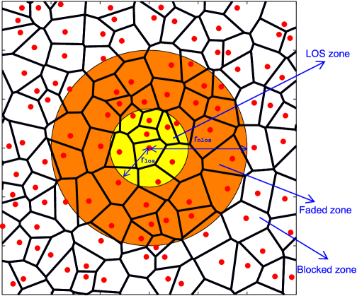
Figure 1: Illustration of a typical network. The BSs are represented by filled red dots, while the tick black lines represents the Voronoi cells. The network is composed of three zones: a) LOS zone, which is the inner circle; b) NLOS or faded zone, which is the annular region colored in orange; c) Blocked zone, which is the region outside the colored circle.

At mmWave frequencies, blockages by various obstacles often prevent LOS propagation, but reflections may allow significant NLOS propagation. In order to model this phenomenon, the propagation model features distance-dependent models for path loss and fading. The local-mean power, which is the average received power at a particular location in the network, is a function of the distance $d$ of the corresponding link. The path-loss function is expressed as the attenuation power law

$$f(d)=\frac{d^{-\alpha(d)}}{d_{0}^{-\alpha(d_{0})}},d\geq d_{0}$$ (1)

where $\alpha(d)$ is the path-loss exponent, and $d_{0}$ is a reference distance that is less than or equal to the minimum of the near-field radius (typically assumed to be line-of-sight).

As shown in Fig. 1, the network is divided into three zones: a) the LOS zone; b) the faded zone; c) and the blocked zone. The LOS zone is a circular region $\mathcal{A}_{\text{los}}$ centered at the reference BS with radius $r_{\mathsf{los}}$ and area $|\mathcal{A}_{1}|=\pi r_{\mathsf{los}}^{2}$. An interfering mobile in this region is assumed to be in the LOS of the reference BS, and its signal is assumed to be subject to additive white Gaussian noise (AWGN) and has path loss $\alpha_{\text{los}}=2$. An interferer within a distance $r_{\mathsf{los}}\leq d\leq r_{\mathsf{nlos}}$ from the reference BS is in the NLOS or faded zone $\mathcal{A}_{\text{nlos}}$. While the signal from a mobile within it might still be harmful and received at the reference BS, it is subject to Rayleigh fading and the path-loss exponent is $\alpha_{\text{nlos}}=4$. An interferer that is beyond distance $r_{\mathsf{nlos}}$ is instead completely blocked, and therefore will not cause any interference.

Each transmitter and receiver within the network is equipped with an antenna array with highly directional beams in order to overcome the high propagation losses and power limitations of mmWave frequencies. Each BS uses fixed sector beams to divide its coverage area into a fixed number of sectors centered at the BS. Each mobile adaptively steers its beam in order to always face its serving BS. At mmWave frequencies, sharp beams can be formed by using many antenna elements. A uniform planar square array (UPA) with half-wavelength antenna element spacing [6, Fig.1(b)] is assumed to be used at each transmitter and receiver. Let $\theta_{\text{bs}}$ and $\theta_{\text{ms}}$ indicate the beamwidth of the antenna main-lobe in the azimuth of the BSs and mobiles, respectively. The antenna gain of the BSs is indicated by $a_{\text{bs}}$, while the antenna gain of the mobiles is $a_{\text{ms}}$. $N_{\text{bs}}$ is the number of antenna elements at each BS, and $N_{\text{ms}}$ is the number of antenna elements equipped at each mobile. The antenna pattern is modeled by a two-level function with maximum gain equal to $G$ over the main-lobe and minimum gain $g$ elsewhere. The values for the beamwidth, main-lobe and back-lobe gains depend on the antenna elements $N$ of the UPA, and can be evaluated per Table I.

TABLE I: Antenna parameters of a uniform planar square antenna.

Number of antenna elements	$N$
Beamwidth $\theta$	$\displaystyle\frac{2\pi}{\sqrt{N}}$
Main-lobe gain $G$	$N$
Side-lobe gain $g$	$\displaystyle\frac{1}{\sin^{2}\left(\frac{3\pi}{2\sqrt{N}}\right)}$

Let $X_{i}=r_{i}e^{j\phi_{i}}$ represent the location of the $i^{th}$ mobile device. For convenience, we represent $X_{i}$ as a complex number, so that $r_{i}=|X_{i}|$ is the distance to the origin (reference BS) and $\phi_{i}$ is the azimuth angle from the BS to the mobile. The gain of the reference sector’s receive antenna in the direction of $X_{i}$ is given by

$$a_{i}=\left\{\begin{array}[c]{cc}G_{\text{bs}},&\mbox{if $|\phi_{i}-\psi|\leq\frac{\theta_{\text{bs}}}{2}$}\\ g_{\text{bs}},&\text{otherwise}\end{array}\right.$$ (2)

where $\psi$ is the offset angle of the beam pattern (i.e., the direction the antenna is pointing). Similarly, the transmit antenna gain of $X_{i}$ in the direction of the reference receiver is

$$b_{i}=\left\{\begin{array}[c]{cc}G_{\text{ms}},&\mbox{if $\left|\phi_{i}-\angle(Y_{g(i)}-X_{i})\right|\leq\frac{\theta_{\text{ms}}}{2}$}\\ g_{\text{ms}},&\text{otherwise}\end{array}\right.$$ (3)

where $g(i)$ denotes a function that returns the index of the BS serving $X_{i}$, and $\angle(Y_{g(i)}-X_{i})$ is the angle from the BS serving $X_{i}$ to $X_{i}$. By assuming that the BS $Y_{g(i)}$ that serves mobile $X_{i}$ is the one with minimum local-mean path loss when the main-lobe of the transmit beam of $X_{i}$ is aligned with the sector beam of $Y_{g(i)}$, the serving BS has index

$$g(i) = \arg\!\max_{j}{\left\{f\left(|Y_{j}-X_{i}|\right)\right\}}.$$ (4)

A frequency-hopping [12] SC-FDMA uplink system is considered. Assuming the mobiles properly advance their signal transmissions, synchronous orthogonal frequency-hopping patterns can be allocated so that at any given instant in time, there is no intra-sector interference. The frequency-hopping patterns transmitted by mobiles in other cells (or sectors) are not generally orthogonal to the patterns in the reference sector, and hence produce inter-cell interference. In this paper, for the sake of tractability, it is assumed that all cells are synchronous and propagation delays are neglected. Thus, when an inter-cell collision occurs (i.e., the mobiles in two different cells select the same hopping frequency), the collision persists for the entire slot; partial collisions are not considered here.

While a reference mobile is located within the reference sector, the potential interfering mobiles are drawn from a PPP $\Phi$, which has intensity $\lambda_{\text{ms}}$ over the entire network except within the reference cell sector area $\mathcal{A}_{\text{sec}}$, where the intensity is zero. Mobiles are randomly re-located each time there is a frequency hop. This assumes a large number of hops/users, and ignores the possibility that the same interferer could be colliding with the reference link multiple times during the same codeword.

The mobile hops $L$ times per codeword. Assuming that full power control is used, the signal-to-interference-and-noise ratio (SINR) for a given codeword is

$$\gamma = \frac{\sum_{t=1}^{L}h_{0,t}}{\mathsf{SNR}^{-1}+\sum_{t=1}^{L}I_{t}}$$ (5)

where $\displaystyle\mathsf{SNR}$ is the signal-to-noise ratio (SNR) and $h_{0,t}$ is the fading gain of the reference link during the $t^{th}$ hop, which is assumed to be gamma distributed with a large Nakagami-m factor $m_{\text{los}}$ as it is assumed that the reference link is LOS. $I_{t}$ is the contribution from the interference during the $t^{th}$ hop. By separating the LOS and NLOS interfering contribution, it can be written as

$$I_{t} = \sum_{i\in\Phi_{\mathsf{los}}^{t}}\Omega_{i}+\sum_{i\in\Phi_{\mathsf{nlos}}^{t}}h_{i,t}\Omega_{i}$$ (6)

where $\Phi_{\mathsf{los}}^{t}$ is the set of LOS interferers during hop $t$, $\Phi_{\mathsf{nlos}}^{t}$ is the set of NLOS interferers during hop $t$. $h_{i,t}$ is the Rayleigh fading power of the $i^{th}$ NLOS interferer during the $t^{th}$ hop, which is modeled as an exponential random variable. $\Omega_{i}$ is the normalized power of the $i^{th}$ transmitter received at the reference BS, given by

$$\Omega_{i} = \frac{1}{L}\frac{a_{i}b_{i}}{G_{\text{bs}}G_{\text{ms}}}\frac{f\left(|X_{i}|\right)}{f\left(|Y_{g(i)}-X_{i}|\right)}.$$ (7)

III Conditional Outage Probability

Let $\beta$ denote the minimum SINR required for reliable reception of a codeword. An outage occurs when the SINR falls below $\beta$. The value of $\beta$ is related to the maximum achievable code rate $R$ that can be achieved. Conditioning over the location of the interferers and BSs (which is embodied by the set $\mathbf{\Omega}=\{\Omega_{i}\}$), the outage probability averaged over the fading and frequency hopping is

$$p_{\mathsf{o}|\bf\Omega} = \mathbb{P}\left[\gamma<\beta\right|\bf\Omega]$$ (8)

Define

$$h = \sum_{t=1}^{L}h_{0,t}$$ (9)

Since $h_{0,t}$ is gamma distributed with parameter $m_{\text{los}}$, $h$ is still gamma distributed but with parameter $M=m_{\text{los}}L$. Therefore, the outage probability can then be expressed as

$$p_{\mathsf{o}|\bf\Omega} = \mathbb{P}\left[h<\beta\left(\mathsf{SNR}^{-1}+\sum_{t=1}^{L}I_{t}\right)\right]$$ (10)

$$= \mathbb{E}_{\bf h}\left[F_{h}\left(\beta\left(\mathsf{SNR}^{-1}+\sum_{t=1}^{L}I_{t}\right)\right)\right]$$

where $\mathbb{E}_{\bf h}\left[\cdot\right]$ is the average over the set of fading gains $\{h_{it}\}$ for the NLOS interferers, and $F_{h}\left(\cdot\right)$ is the cumulative distribution function (CDF) of $h$. For a normalized gamma distributed random variable $Z$ with (integer) parameter $m$, the CDF evaluated at a point $z$ can be tightly lower bounded [13] as follows

$$F_{Z}(z) = \left(1-\exp\left\{-m(m!)^{\frac{-1}{m}}z\right\}\right)^{m}$$ (11)

Substituting (11) into (10) and defining $\tilde{M}={(M!)^{\frac{-1}{M}}}$ yields

$$p_{\mathsf{o}|\bf\Omega} = \mathbb{E}_{\bf h}\left[\left(1-e^{-M\tilde{M}\beta\left(\mathsf{SNR}^{-1}+\sum_{t=1}^{L}I_{t}\right)}\right)^{M}\right]$$ (12)

Substituting (6) in (12) and performing a binomial expansion,

$$p_{\mathsf{o}|\bf\Omega} = 1-\sum_{l=1}^{M}{{M}\choose{l}}\left(-1\right)^{l+1}\times$$ (13)

$$\exp{\left[-lM\tilde{M}\beta\left(\mathsf{SNR}^{-1}+\sum_{t=1}^{L}\sum_{i\in\Phi_{\mathsf{LOS}}^{t}}\Omega_{i}\right)\right]}\times$$

$$E_{\mathbb{h}}\left[\exp{\left(-lM\tilde{M}\beta\sum_{t=1}^{M}\sum_{i\in\Phi_{\mathsf{NLOS}}^{t}}h_{i,t}\Omega_{i}\right)}\right].$$

Using the fact that the set of fading gains $\{h_{i,t}\}$ are independently and identically distributed (iid), then (13) can be written as follows

$$p_{\mathsf{o}|\bf\Omega} = 1-\sum_{l=1}^{M}{{M}\choose{l}}\left(-1\right)^{l+1}\times$$ (14)

$$\exp{\left[-lM\tilde{M}\beta\left(\mathsf{SNR}^{-1}+\sum_{t=1}^{L}\sum_{i\in\Phi_{\mathsf{LOS}}^{t}}\Omega_{i}\right)\right]}\times$$

$$\prod_{t=1}^{L}\prod_{i\in\Phi_{\mathsf{NLOS}}^{t}}E_{h_{i,t}}\left[\exp{\left(-lM\tilde{M}\beta h_{i,t}\Omega_{i}\right)}\right].$$

Solving the expectation in (14) for the gamma-distributed $h_{i,t}$ with parameter $m_{\text{nlos}}$ yields

$$p_{\mathsf{o}|\bf\Omega} = 1-\sum_{l=1}^{M}{{M}\choose{l}}\left(-1\right)^{l+1}\times$$ (15)

$$\exp{\left[-lM\tilde{M}\beta\left(\mathsf{SNR}^{-1}+\sum_{t=1}^{L}\sum_{i\in\Phi_{\mathsf{LOS}}^{t}}\Omega_{i}\right)\right]}\times$$

$$\prod_{t=1}^{L}\prod_{i\in\Phi_{\mathsf{NLOS}}^{t}}\left(1+\frac{l\tilde{M}M\beta\Omega_{i}}{m_{\text{nlos}}}\right)^{-m_{\text{nlos}}}.$$

TABLE II: Settings used.

Faded zone outer radius	$r_{\text{nlos}}=10$
LOS zone radius	$r_{\text{los}}=2$
Distribution for the BSs	UCP with $r_{\text{min}}=1$
Distribution of the mobiles	PPP
Intensity of BSs	$\lambda_{\text{bs}}=0.2$
Intensity of mobiles	$\lambda_{\text{ms}}=1$
Path loss exponent	$\alpha_{\text{los}}=2$ and $\alpha_{\text{nlos}}=4$
Fading parameters	$m_{\text{los}}=3$ and $m_{\text{nlos}}$=1
Reference distance	$d_{0}=0.01$
Signal-to-noise ratio	$\displaystyle\mathsf{SNR}=25$ dB
Antenna elements at the BS	$N_{\text{bs}}=256$
Antenna elements at the mobile	$N_{\text{ms}}=16$
Number of frequency hops	$L=2$
Outage contraint	$\hat{\epsilon}=0.1$
Network trials	$N_{\text{trials}}=10^{6}$

IV Spatially Averaged Outage Probability

Typical analyses based on stochastic geometry find the outage probability averaged over the network topology. Since the locations of the mobile stations change more frequently than the locations of the BSs, a sensible approach is to find the spatially averaged outage probability of the network by first averaging over the locations of the mobiles, then averaging over the locations of the BSs. As the locations of the mobiles are contained in the point process $\Phi$, the outage probability conditioned on only the locations of the BSs, but averaged over the locations of the mobiles, can be written as

$$p_{\mathsf{o}|{\bf Y}} = \mathbb{P}\left[\gamma<\beta\right|{\bf Y}]=\mathbb{E}_{\Phi}\left[p_{\mathsf{o}|\bf\Omega}\right].$$ (16)

where $\mathbf{Y}$ is the set of BS locations.

Substituting (15) into (16) yields

$$p_{\mathsf{o}|\bf Y} = 1-\sum_{l=1}^{M}{{M}\choose{l}}\left(-1\right)^{l+1}\times$$ (17)

$$\exp{\left[-lM\tilde{M}\beta\left(\mathsf{SNR}^{-1}+L\mathcal{E}_{1}\right)\right]}\mathcal{E}_{2}^{L}$$

where

$$\mathcal{E}_{1} = \mathbb{E}_{\Phi}\left[\sum_{i\in\Phi_{\mathsf{LOS}}^{t}}\Omega_{i}\right]$$

$$\stackrel{{\scriptstyle a}}{{=}} \lambda_{mb}\left(|\mathcal{A}_{1}|-|\mathcal{A}_{\text{sec}}|\right)\mathbb{E}_{X}\left[\Omega_{i}\right]$$

$$\mathcal{E}_{2} = \mathbb{E}_{\Phi}\left[\prod_{i\in\Phi_{\mathsf{NLOS}}^{t}}\left(1+\frac{l\tilde{M}M\beta\Omega_{i}}{m_{\text{nlos}}}\right)^{-m_{\text{nlos}}}\right]$$

$$\stackrel{{\scriptstyle b}}{{=}} \exp\left\{-\lambda_{mb}|\mathcal{A}_{2}|\left(1-\mathbb{E}_{X}\left[\left(1+\frac{l\tilde{M}M\beta\Omega_{i}}{m_{\text{nlos}}}\right)^{-m_{\text{nlos}}}\right]\right)\right\}$$

where $(\stackrel{{\scriptstyle a}}{{=}})$ and $(\stackrel{{\scriptstyle b}}{{=}})$ are obtained using a similar approach of that taken in [14] by using the fact that the mobiles are independently and uniformly distributed, and the number of mobiles within an area is a Poisson random variable. For both $\mathcal{E}_{1}$ and $\mathcal{E}_{2}$, the final expression reduces to the evaluation of $E_{X}\left[\cdot\right]$, which is the average with respect to the location $X$ of a single mobile. These two averages can be obtained either by Monte Carlo simulation (by simulating the location of a mobile within $\mathcal{A}_{1}\backslash\mathcal{A}_{\text{sec}}$ and $\mathcal{A}_{2}$, respectively) or by using numerical integration after the distribution of the CDF of the normalized received power is evaluated using the approach provided in [15].

Having averaged the outage probability over the locations of the mobiles, the outage probability averaged over the locations of the BSs can be found, if so desired, by averaging (16) over the spatial distribution of the BSs. The average outage probability is hence

$$p_{\mathsf{o}} = \mathbb{P}\left[\gamma<\beta\right]=\mathbb{E}_{Y}\left[p_{\mathsf{o}|\bf Y}\right].$$ (18)

In order to evaluate $p_{\mathsf{o}}$, a Monte Carlo approach can be used. After a large set of network topologies, say $N_{\text{trial}}$ network realizations, is created, (17) is evaluated and saved for each realization, and these values are used to evaluate $p_{\mathsf{o}}$ by computing their average. Arguably, a more useful quantity that the overall average outage probability is the distribution of $p_{\mathsf{o}|\bf\Omega}$, which gives insight into the number of network realizations (or the number of reference sectors in a large network) that achieve a target outage probability; such a distribution can also be found using Monte Carlo methods, as shown in the next section.

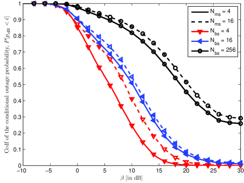
Figure 2: CCDF of the conditional outage probability $p_{\mathsf{o}|\bf\Omega}$ as function of the SINR threshold. Curves are parameterized over the antenna elements equipped at both the BS and mobile.

V Numerical Results

This section evaluates the performance of a 5G mmWave uplink by computing the CCDF of the conditional outage probability $p_{\mathsf{o}|\bf\Omega}$. In particular, the CCDF of $p_{\mathsf{o}|\bf\Omega}$ is used to depict the percentage of the mobiles that have an outage probability below a given outage constraint $\hat{\epsilon}$, i.e $\mathbb{P}\left[p_{\mathsf{o}|\bf\Omega}<\hat{\epsilon}\right]$. While $p_{\mathsf{o}|\bf\Omega}$ can be evaluated analytically using (15), its distribution is computed using a Monte Carlo approach by randomly varying at each of the $N_{\text{trial}}$ trials the topology of the network according to the spatial distribution of both the mobiles and the BSs.

Another useful metric is the area spectral efficiency (ASE). This metric provides the maximum rate of successful data transmissions per unit area, and it is defined as

$$\tau_{\text{ASE}} = \lambda_{\text{bs}}R\left(1-p_{\mathsf{o}}\right)$$ (19)

where the units are bits per channel use (bpcu) per unit area. If a capacity approaching code is assumed to be used and rate adaptation is performed over a large set of modulation and coding schemes, the code rate $R$ can be related to the SINR threshold using the Shannon bound for complex discrete-time AWGN channels, as follows

$$R = \log_{2}\left(1+l_{s}\beta\right)$$ (20)

where $l_{s}=0.794$ to account for the typical $1$ dB loss from Shannon capacity of an actual code.

In the following example, the settings summarized in Table II are adopted, if not otherwise stated. Fig. 2 shows the CCDF of the conditional outage probability $p_{\mathsf{o}|\bf\Omega}$ as function of the SINR threshold when the BS and the mobile are equipped with a different number of antenna elements. This figure highlights the importance of sectorization, and that a small improvement is gained by equipping large arrays of antennas at the mobile.

Fig. 3 compares the performance of the network in terms of the number of hops per codeword, again by showing the CCDF of the conditional outage probability $p_{\mathsf{o}|\bf\Omega}$ as function of the SINR threshold. This figure shows that the percentage of mobiles that are able to satisfy an outage constraint $\hat{\epsilon}$ sensibly increases as the number of hops per codeword is increased emphasizing the role of frequency-hopping in reducing the power level of the inter-cell interferers.

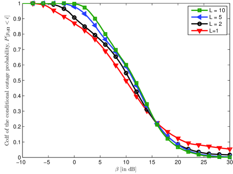
Figure 3: CCDF of the conditional outage probability $p_{\mathsf{o}|\bf\Omega}$ as function of the SINR threshold. Curves are parameterized over the number of frequency hops per codeword.

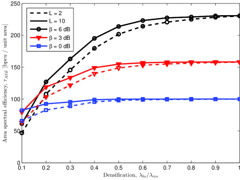
Figure 4: ASE as function of densification of the BSs. Curves are parameterized by both the SINR threshold and the number of frequency hops per codeword.

Fig. 4 provides the ASE as the network densifies by deploying a larger number of BSs. This figure shows the importance of densification. Increases in the SINR threshold $\beta$ degrade the outage probability. However, for a sufficiently densified network this effect is minor compared with increased code rate that can be accommodated. As a result, the area spectral efficiency $\tau_{\text{ASE}}$ increases significantly. Furthermore, as the network becomes more densified a lower power is required for each intended link due to power control, and therefore the power level of the interference decreases with the consequence that aggressive hopping doesn’t provide any significant improvement.

VI Conclusions

This paper derives an analytical framework to evaluate the outage probability for mmWave uplink cellular networks when frequency-hopping is adopted. The model includes the effects of mmWave propagation, highly directional beams, and arbitrary network topologies. Results emphasize the importance of BS densification, and sectorization. Furthermore, the beneficial effects of frequency-hopping are illuminated by the analysis, and frequency hopping seems to be a good complement to the use of power control and directional antennas.

REFERENCES

- [1] J. G. Andrews, S. Buzzi, C. Wan, S. V. Hanly, A. Lozano, A. C. K. Soong, and J. C. Zhang, “What will 5G be?,” IEEE J. Select. Areas Commun., vol. 32, pp. 1065–1082, June 2014.
- [2] S. Rangan, T. Rappaport, and E. Erkip, “Millimeter-wave cellular wireless networks: Potentials and challenges,” Proc. IEEE, vol. 12, pp. 366–385, March 2014.
- [3] Y. Niu, Y. Li, D. Jin, L. Su, and A. V. Vasilakos, “A survey of millimeter wave communications (mmwave) for 5G: opportunities and challenges,” Wireless Networks, vol. 21, pp. 2657–2676, November 2015.
- [4] T. S. Rappaport, S. Sun, R. Mayzus, H. Zhao, Y. Azar, K. Wang, G. N. Wong, J. K. Schultz, M. Samimi, and F. Gutierrez, “Millimeter wave mobile communications for 5g cellular: It will work!,” IEEE Access, vol. 1, pp. 335–349, November 2013.
- [5] M. R. Akdeniz, Y. Liu, M. K. Samimi, S. Sun, S. Rangan, T. S. Rappaport, and E. Erkip, “Millimeter wave channel modeling and cellular capacity evaluation,” IEEE J. Select. Areas Commun., vol. 32, pp. 1164–1179, June 2014.
- [6] T. Bai and R. W. Heath Jr., “Coverage and rate analysis for millimeter wave cellular networks,” IEEE Trans. Wireless Comm., vol. 14, pp. 1100–1114, October 2014.
- [7] M. Di Renzo, “Stochastic geometry modeling and analysis of multi-tier millimeter wave cellular networks,” IEEE Trans. Wireless Comm., vol. 14, pp. 5038–5057, September 2015.
- [8] E. Turgut and M. C. Gursoy, “Average error probability analysis in mmwave cellular networks,” in Proc. IEEE Veh. Tech. Conf. (VTC), (Boston, MA), September 2015.
- [9] S. Singh, M. N. Kulkarni, A. Ghosh, and J. G. Andrews, “Tractable model for rate in self-backhauled millimeter wave cellular networks,” IEEE J. Select. Areas Commun., 2015. Available: http://arxiv.org/pdf/1407.5537v1.pdf.
- [10] D. Torrieri, S. Talarico, and M. C. Valenti, “Performance analysis of fifth-generation cellular uplink,” in Proc. IEEE Military Commun. Conf. (MILCOM), (Tampa, FL), Oct. 2015.
- [11] D. Torrieri, M. C. Valenti, and S. Talarico, “An analysis of the DS-CDMA cellular uplink for arbitrary and constrained topologies,” IEEE Trans. Commun., vol. 61, pp. 3318–3326, Aug. 2013.
- [12] D. Torrieri, Principles of Spread-Spectrum Communication Systems, 3nd ed. New York: Springer, 2015.
- [13] H. Alzer, “On some inequalities for the incomplete gamma function,” Mathematics of Computation, vol. 66, pp. 771–778, Apr. 1997.
- [14] M. C. Valenti, D. Torrieri, and S. Talarico, “A direct approach to computing spatially averaged outage probability,” IEEE Commun. Letters, vol. 18, pp. 1103–1106, July. 2014.
- [15] R. Pure and S. Durrani, “Computing exact closed-form distance distributions in arbitrarily-shaped polygons with arbitrary reference point,” The Mathematica Journal, vol. 17, pp. 1–27, June 2015.