Mesh Adaptation on the Sphere using Optimal Transport and the Numerical Solution of a Monge-Ampère type Equation

Abstract

Graphical abstract

An equation of Monge-Ampère type has, for the first time, been solved numerically on the surface of the sphere in order to generate optimally transported (OT) meshes, equidistributed with respect to a monitor function. Optimal transport generates meshes that keep the same connectivity as the original mesh, making them suitable for r-adaptive simulations, in which the equations of motion can be solved in a moving frame of reference in order to avoid mapping the solution between old and new meshes and to avoid load balancing problems on parallel computers.

The semi-implicit solution of the Monge-Ampère type equation involves a new linearisation of the Hessian term, and exponential maps are used to map from old to new meshes on the sphere. The determinant of the Hessian is evaluated as the change in volume between old and new mesh cells, rather than using numerical approximations to the gradients.

OT meshes are generated to compare with centroidal Voronoi tesselations on the sphere and are found to have advantages and disadvantages; OT equidistribution is more accurate, the number of iterations to convergence is independent of the mesh size, face skewness is reduced and the connectivity does not change. However anisotropy is higher and the OT meshes are non-orthogonal.

It is shown that optimal transport on the sphere leads to meshes that do not tangle. However, tangling can be introduced by numerical errors in calculating the gradient of the mesh potential. Methods for alleviating this problem are explored.

Finally, OT meshes are generated using observed precipitation as a monitor function, in order to demonstrate the potential power of the technique.

1 Introduction

The need to represent scale interactions in weather and climate prediction models has, for many decades, motivated research into the use of adaptive meshes [3, 35, 39]. R-adaptivity - mesh redistribution - involves deforming a mesh in order to vary local resolution and was first considered for atmospheric modelling more than twenty years ago by Dietachmayer and Droegemeier [15]. It is an attractive form of adaptivity since it does not involve altering the mesh connectivity, does not create load balancing problems because points are never created or destroyed, does not require mapping of solutions between meshes [27], does not lead to sudden changes in resolution and can be retro-fitted into existing models. Variational methods exist which attempt to control resolution in different directions for r-adaptive meshes [eg 24, 26]. Alternatively, the solution of the Monge-Ampère equation to generate an optimally transported (OT) mesh based on a scalar valued monitor function is a useful form of r-adaptive mesh generation because it generates a mesh equidistributed with respect to a monitor function and does not lead to mesh tangling [7]. We will see that the optimal transport problem on the sphere leads to a slightly different equation of Monge-Ampère type, which has not before been solved numerically on the surface of a sphere, which would be necessary for weather and climate prediction using r-adaptivity.

At first glance, r-adaptivity does not look ideal for adaptive meshing of the global atmosphere; Dietachmayer and Droegemeier [15] pointed out that the resulting meshes can be quite distorted which leads to truncation errors and it is not always possible to control the resolution in individual directions, just the total cell size (area or volume); with r-adaptivity, it is not possible, for example, to increase the total number of points around the equator, just re-distribute them [18]. However, if the mesh redistribution starts from a mesh with enough points around the equator, then these points can be redistributed according to transient features of the flow.

Models of the global atmosphere are being developed with accurate treatment of non-orthogonality and which allow arbitrary grid structures [22, 30, 12, 29, 40]. The time may therefore be right to reconsider r-adaptive modelling of the global atmosphere.

A powerful form of adaptivity that, like r-adaptivity, retains the same total number of points, is centroidal Voronoi tesselation using a non-uniform density (or monitor) function to control the mesh spacing, using Lloyd’s algorithm [33]. Lloyd’s algorithm generates smoothly varying, orthogonal, near centroidal isotropic meshes suitable for finite-volume models and is being used by the Model for Prediction Across Scales [MPAS, 36]. Lloyd’s algorithm alters the mesh connectivity meaning that, if it is used in conjunction with dynamic mesh adaptivity, mapping between old and new solutions is needed and there is an additional layer of complexity involved with changing the data structures and moving information between parallel processors. Also, Lloyd’s algorithm is extremely expensive, using an explicit solution to find an equidistributed mesh - an elliptic problem. The cost per iteration is proportional to the number of points, $N$, [25] and, in one dimension, the number of iterations is proportional to $N$ [16]. Therefore, overall, the cost is proportional to $N^{2}$. Conversely, generating optimally transported meshes using a semi-implicit technique, has convergence independent of the mesh size and the overall cost is proportional to $N\log N$ [5]. We therefore propose r-adaptivity which uses cheaper mesh generation and fixed data structures associated with the mesh.

In section 2 we describe mesh generation by optimal transport in Euclidean space leading to a Monge-Ampère equation. We then show how these concepts can extend to mesh generation on the sphere, leading to an equation of Monge-Ampère type. Existing numerical solution techniques in Euclidean geometry are reviewed in section 3. In section 4 we describe the new numerical methods for solving the Monge-Ampère type equations, both on a Euclidean plane and on the sphere. In order to address issues of mesh distortion, a range of diagnostics of mesh quality are presented. These diagnostics, along with the diagnostics of solution convergence, are described in section 5 and the diagnostics of the meshes generated are presented in section 6. The meshes generated, both on the plane and on the sphere, are shown and described in section 6 and the meshes on the sphere are compared with centroidal Voronoi meshes generated using Lloyd’s algorithm [33] with the same monitor function. In order to demonstrate the performance of the mesh generation using real data as a monitor function, meshes are generated using a monitor function derived from reanalysis precipitation in section 6. Final conclusions and recommendations for future work are drawn in section 7.

2 Mesh Generation by Optimal Transport (OT)

2.1 Optimally Transported Meshes in Euclidean Space

A mesh is equidistributed with respect to a monitor function when the product of the cell volumes and the monitor function in the cell is constant across all mesh cells. The equidistribution principle alone does not lead to a well-defined problem for mesh generation. Indeed this problem is ill-posed in more than 1 dimension and so requires the imposition of an extra constraint. Budd and Williams [6] introduced optimal transport for mesh generation to find a map from the original mesh (or computational space, $\Omega_{c}$) to the new mesh (or physical space, $\Omega_{p}$). This technique was further developed by Budd et al. [7] and extended to 3 spatial dimensions by Browne et al. [5]. The optimal transport constraint says that the new mesh should be as close as possible to the original mesh - we seek to minimise the distance between the two meshes in a certain measure which we shall discuss. We write this minimization problem:

$$\min_{\mathbf{x}\in\Omega_{p}}d(\bm{\xi},\mathbf{x})^{2}$$ (1)

where $d$ is the distance metric between the two meshes and $\bm{\xi}\in\Omega_{c}$ maps to $\mathbf{x}\in\Omega_{p}$. In Cartesian space $[0,1]^{n}$ this metric can simply be the sum of the Euclidean distance between all of the corresponding points defining the meshes. Brenier’s theorem [4] then tells us that the unique, optimal transport map from $\mathbf{x}$ to $\bm{\xi}$ is the gradient of a convex scalar potential, $\phi$, so that the new mesh locations are given by:

$${\bf x}=\bm{\xi}+\nabla\phi.$$ (2)

The change in cell volume under the coordinate transform is given by the determinant of the Jacobian of the map, $|J(\xi)|=|\mathbf{\nabla\mathbf{x}}(\bm{\xi})|$, the gradient of $\mathbf{x}$ with respect to $\bm{\xi}$. Therefore, for equidistribution with respect to a monitor function, $m$, the new mesh locations should satisfy

$$|\nabla\mathbf{x}|\ m\left(\mathbf{x}\right)=c$$ (3)

where $c$ is a constant, uniform over space, which will be determined once the numerical method is defined. Taking the determinant of the gradient of eqn. (2), we can see that $|\nabla\mathbf{x}|=|I+\nabla\nabla\phi|=|I+H\left(\phi\right)|$ where $I$ is the identity tensor and $H$ is the Hessian. Consequently, for the mesh to be optimally transported and equidistributed, the mesh potential, $\phi$, must satisfy a Monge-Ampère equation:

$$|I+H\left(\phi\right)|m({\bf x})=c.$$ (4)

The presence of the identity tensor in this Monge-Ampère equation will be exploited in the linearisation to create a novel numerical algorithm.

Mesh tangling is caused by a local loss of invertibility of the Jacobian of the map from the original to the tranported mesh. Given that the solution of the Monge-Ampère equation, $\phi$, is convex, the determinant of the Hessian of $\phi$ is positive and hence the Jacobian determinant of the map is positive and thus is invertible and the mesh will not tangle [7].

2.2 Optimally Transported Meshes on the Sphere

A naive approach to r-adaptivity on the sphere, $\mathbb{S}^{2}$, would be to map the surface onto the plane, use an established method to solve a mesh redistribution problem on the plane, then map back to the sphere. As shown in Figure 1, the desired map $T$ could be written as a composition of mappings as $T=g^{-1}\circ t\circ g$.

Figure 1: Commutative diagram showing an naive approach to meshing on the sphere by converting the problem to the plane

A map $g:\mathbb{S}^{2}\to\mathbb{R}^{2}$ must be chosen and an optimal transport map $t$ found. The boundary conditions for the problem of finding $t$ must be specified, and those boundary conditions would necessarily depend on $g$. For example in the case where the mapping $g$ is simply the lat-lon decomposition of $\mathbb{S}^{2}$, the boundary conditions for the mesh redistribution problem on the plane will then be periodic in the zonal direction. In the the meridional direction, Neumann boundary conditions would not be appropriate as the poles will not be free to move and they will be mapped back to their original location under $g^{-1}$.

The Hairy Ball Theorem tells us that there must be at least one fixed point of the map $T:\mathbb{S}^{2}\to\mathbb{S}^{2}$. The decomposition $T=g^{-1}\circ t\circ g$ would then be possible if $g$ maps the fixed points of $T$ to a Neumann boundary of $\mathbb{R}^{2}$. However the location of the fixed points of $T$ are not known a priori, and hence choosing $g$ appropriately would form a significant problem by itself. Hence we will seek a direct optimal transport map, $T:\mathbb{S}^{2}\to\mathbb{S}^{2}$ which will be described in this section.

On the surface of the sphere, we would still like to define an optimally transported mesh satisfying equidistribution:

$$r\left(\phi\right)m\left(\bm{x}\right)=c$$ (5)

where $r=V_{\xi}/V_{x}$ is the ratio of the volumes of the original mesh cells, $V{}_{\xi}$, with vertices at positions $\bm{\xi}$, and the volumes of the new mesh cells, $V_{x}$, with vertices at positions $\bm{x}$. We need to ascertain if unique solutions of (5) exist which minimise the distance between the original and resulting meshes. On the sphere $\mathbb{S}^{2}$, the appropriate distance metric is the Riemannian distance on the surface of the sphere between all of the corresponding points defining the meshes. We cannot use Brenier’s theorem on the sphere. Instead, we appeal to the generalised version of Brenier’s theorem given by McCann [28], a detailed discussion of which is given in Villani [38].

Definition 1.

[$c$-convex function] The $c$-transform $\phi^{c}$ of a function $\phi:\mathbb{S}^{2}\to\mathbf{\mathbb{R}}$ is defined as

$$\phi^{c}(y)=\sup_{\bm{\xi}\in\mathbf{\mathbb{S}}^{2}}\{-c(\bm{\xi},\mathbf{x})-\phi(\bm{\xi})\}.$$ (6)

The function $\phi$ is said to be $c$-convex, or cost-convex, if $(\phi^{c})^{c}=\phi.$

Theorem 1.

(A combination of theorems 8 and 9 of[28]) Let $M$ be a connected, complete smooth Riemannian manifold, equipped with its standard volume measure $\mathrm{d}x$. Let $\mu,\nu$ be two probability measures on $M$ with compact support, and let the objective function $c(\bm{\xi},\mathbf{x})$ be equal to $d(\bm{\xi},\mathbf{x})^{2}$, where $d$ is the geodesic distance on $M$. Further, assume that $\mu$ is absolutely continuous with respect to the volume measure on $M$. Then, the Monge-Kantorovich mass transportation problem between $\mu$ and $\nu$ admits a unique optimal transported map $T$ where $T$ pushes forward the measure $\mu$ onto $\nu$. Then, (using classical optimal transport notation):

$$T_{\#}\mu=\nu$$ (7)

such that

$$\mathbf{x}=T(\bm{\xi})=\exp_{\bm{\xi}}[\nabla\phi(\bm{\xi})]$$ (8)

for some $d^{2}/2$-convex potential $\phi$.

Corollary 1.

There exists a unique, optimally transported mesh on the sphere that satisfies the equidistribution principle. Moreover, that mesh is defined by a $c$-convex scalar potential function that satisfies the Monge-Ampère type equation

$$m\left(\exp_{\xi}[\nabla\phi(\bm{\xi})]\right)|J(\bm{\xi})|=c.$$ (9)

Proof.

Clearly $M=\mathbb{S}^{2}$ satisfies the conditions on $M$ in Theorem 1. The first probability measure of interest, $\mu$, we define to be the scaled Lebesgue measure such that:

$$\mathrm{d}\mu=\frac{\mathrm{d}x}{\int_{\mathbb{S}^{2}}\mathrm{d}x}.$$ (10)

The target probability measure, $\mu$, is the Lebesgue measure appropriately scaled by the monitor function to be equidistribed, such that:

$$\mathrm{d}\nu=\frac{m(\mathbf{x})\mathrm{d}x}{\int_{\mathbb{S}^{2}}m(\mathbf{x})\ \mathrm{d}x}.$$ (11)

As $M=\mathbb{S}^{2}$ these are trivially compactly supported. $\mu$ is absolutely continuous. Hence by Theorem 1 we have that there exists a unique solution, $T$, to the mass transportation problem between $\mu$ and $\nu$. From (8) we can see that any point in the new mesh, $\mathbf{x}$, is defined by the action of the exponential map on the scalar potential, $\phi$.

To see that this map, $T$, will give a mesh that satisfies the equidistribution principle, consider a cell $A_{\xi}$ in the original computational mesh, $\Omega_{C}$ with volume $V_{\xi}$. The mapping of the cell under $T$ gives the new cell, $A_{x}$ in the physical mesh $\Omega_{p}$. As $T$ is a (optimal) transport map, then the integral over a set with respect to the measure $\mu$ equals the integral over the image of that set with respect to $\nu$. Hence:

$$\int_{A_{\xi}}\mathrm{d}\mu=\int_{A_{x}}\mathrm{d}\nu\implies\frac{V_{\xi}}{\int_{\mathbb{S}^{2}}\mathrm{d}x}=\frac{\int_{A_{x}}m(\mathbf{x})\ \mathrm{d}x}{\int_{\mathbb{S}^{2}}m(\mathbf{x})\ \mathrm{d}x}.$$ (12)

The ratio of the integral of the monitor function over the new cell with the total integral of the monitor function is equal to the proportion of the volume that the original cell occupied in the original mesh. This is precisely what it means for the monitor function to be equidistributed on a discretised mesh.

Using a change of variables, we have:

$$\frac{V_{\xi}}{\int_{\mathbb{S}^{2}}\mathrm{d}x}=\frac{\int_{A_{x}}m(\mathbf{x})\ \mathrm{d}x}{\int_{\mathbb{S}^{2}}m(\mathbf{x})\ \mathrm{d}x}=\frac{\int_{A_{\xi}}m(\exp_{\xi}[\nabla\phi(\bm{\xi})])|J(\bm{\xi})|\ \mathrm{d}\xi}{\int_{\mathbb{S}^{2}}m(\mathbf{x})\ \mathrm{d}x}$$ (13)

where $|J(\bm{\xi})|$ is the determinant of the Jacobian of the map $T(\bm{\xi})=\exp_{\xi}[\nabla\phi(\bm{\xi})]$.

As (13) must hold for arbitrary sets $A_{\xi}\in\Omega_{C}$, the following equation of Monge-Ampère type on the sphere results:

$$m\left(\exp_{\xi}[\nabla\phi(\bm{\xi})]\right)|J(\bm{\xi})|=\frac{\int_{\mathbb{S}^{2}}m(\mathbf{x})\ \mathrm{d}x}{\int_{\mathbb{S}^{2}}\mathrm{d}x}=c.$$ (14)

∎

Corollary 2.

The optimally transported mesh on the sphere satisfying the equidistribution principle does not exhibit tangling.

Proof.

The choice of cost function $c$ to be the squared geodesic distance is crucial to the proof of uniqueness in Theorem 1. Indeed simply taking $c$ to be the square of the Euclidean distance is not sufficient [1]. The squared geodesic distance is necessary to ensure that the classical twist condition holds, i.e. $T$ given in (7) is injective and hence is a map.

The injectivity of this map ensures that (8) is locally invertible, i.e. for each point in the new mesh, $\mathbf{x}$, there is a unique point in the original mesh, $\bm{\xi}$, which maps to it - i.e. mesh tangling is not present. ∎

3 A Review of Numerical Methods for solving the Monge-Ampère Equation

The fully non-linear, second-order, elliptic Monge-Ampère equation is:

$$|H\left(\phi\left(\bm{\xi}\right)\right)|=f\left(\bm{\xi},\phi\right)$$ (15)

for independent variable $\bm{\xi}\in\Omega$ and $\Omega\subset\mathbb{R}^{d}$ where $\phi$ is the (scalar) dependent variable, $f$ is a known scalar function of $\bm{\xi}$ and $\phi$, $H=\nabla\nabla$ is the Hessian (the tensorial gradient of the gradient) and $|H|$ is the determinant of the Hessian. Froese and Oberman [20] give an excellent review of some numerical methods for solving this equation and this review draws from and adds to their review.

There are two challenging parts to solving the Monge-Ampère equation. Firstly we need spatial discretisation methods both for the Hessian, $H$, and for the source term, $f$ (although $f$ is a known function, it can be a function of $\phi$ or of $\nabla\phi$, so numerical approximations are necessary). The spatial discretisation leads to a set of non-linear algebraic equations. Secondly, the algebraic equations require a numerical algorithm to find solutions. The discretisation should ensure that the solutions is convex based on a discrete definition of convexity. We will start by considering the spatial discretisation of the Hessian, $H$.

Budd et al. [7] used finite differences on a structured, Cartesian grid to discretise the Hessian, a technique that was extended to three dimensions by Browne et al. [5]. Convexity was ensured by filtering the monitor function and smoothing the non-converged solution. Oberman [31] describe a finite difference method that uses a wide stencil to calculate the Hessian on a structured Cartesian grid. This was extended to three dimensions by Froese and Oberman [20]. The wide stencil was needed to ensure monotonicity of the iterative solution to the convex, numerical solution. Froese et al. [21] study the slightly different, 2-Hessian equation and describe how they rotate the coordinate system so that the Hessian is diagonal and hence the solution is convex and the discretisation is monotone. Feng and Neilan [17] approximate the Monge-Ampère equation by a fourth-order quasi-linear equation in order to use mixed finite elements for the spatial discretisation. Dean and Glowinski [13, 14] also use mixed finite-elements on triangulations of the unit plane. All of these techniques have been used on either 2D or 3D Euclidean geometry.

When solving the Monge-Ampère equation for mesh adaptation, the RHS of eqn (15) depends on $\nabla\phi$. Froese [19] pointed out that standard centred differences are not monotone for discretising this term and so used wide stencil finite differences. Saumier et al. [34] experimented with second and fourth order centred finite differences and a spectral method for discretisting $\nabla\phi$.

Once the Monge-Ampère equation is discretised in space, it is necessary to solve the resulting non-linear algebraic equations, the part of the method that we describe as the “algorithm”. Budd and Williams [6], Budd et al. [7] introduced a parabolic version of the Monge-Ampère equation which is solved by time-stepping, including an implicit relaxation term to smooth the transient solution and to speed up convergence:

$$\left(I-\gamma\nabla^{2}\right)\frac{\partial\phi}{\partial t}=\left(m\left(\nabla\phi\right)|I+H\left(\phi\right)|\right)^{\frac{1}{d}}$$ (16)

where $\gamma$ is a scalar parameter defining the amount of smoothing applied, $\nabla^{2}$ is the Laplacian operator and $d$ is the number of spatial dimensions. The time-stepping effectively creates fixed-point iterations but it may be possible to create more convergent iterations, without smoothing towards a uniform mesh. Benamou et al. [2] also used fixed-point iterations by linearising the two-dimensional Hessian term with a Laplacian:

$$|H\left(\phi\right)|=\frac{1}{2}\left(\nabla^{2}\phi\right)^{2}-\frac{\phi_{xx}^{2}+\phi_{yy}^{2}}{2}-\phi_{xy}^{2}.$$ (17)

After some manipulation, this results in a Poisson equation which can be solved implicitly with the non-linear terms on the right hand side. Froese and Oberman [20] describe this as a semi-implicit method and use it to find the starting point for a Newton method. A Newton method is a common algorithm for solving the algebraic equations [13, 20, 11]. However the cost and complexity of the Newton method may not be necessary for mesh generation. In this paper we focus on fixed-point iterations, although the new linearisation proposed may also be beneficial for calculating the first guess for a Newton method.

Equations of Monge-Ampère type have not before been solved numerically on the sphere. The description of the optimally transported mesh problem using the Monge-Ampère equation relies on properties of Euclidean geometry [7]. The numerical solution technique for the optimal transport problem on the surface of a sphere will be described in section 4.

4 Numerical Method for Calculating OT Meshes

There are two aspects to solving equations of Monge-Ampère type in order to calculate optimally transported (OT) meshes. The spatial discretisation describes how to calculate the gradient and the Hessian of the mesh potential, $\phi$, from discrete values (in this instance in finite volume cells). This will convert the PDE into a set of non-linear algebraic equations. The algorithm describes how to linearise and solve the large set of non-linear algebraic equations.

4.1 The Numerical Algorithm

4.1.1 In Euclidian Space

A fixed-point iteration sequence to solve eqn. (4) can be found by observing that the linear terms of $|I+H\left(\phi\right)|$ are in fact $1+\nabla^{2}\phi$ where $\nabla^{2}$ is the Laplacian operator (linearising about $\phi=0$). Eqn. (4) can then be written as fixed-point iterations:

$$1+\nabla^{2}\phi^{n+1}=1+\nabla^{2}\phi^{n}-|I+H\left(\phi^{n}\right)|+\frac{c^{n}}{m({\bf x}^{n})}$$ (18)

where $n$ is the iteration number and where:

$${\bf x}^{n}=\bm{\xi}+\nabla\phi^{n}.$$ (19)

This is simpler than the fixed-point iterations used by Feng and Neilan [17], Benamou et al. [2] because of the presence of the identity tensor in our Monge-Ampère equation which simplifies the linearisation. These fixed-point iterations are similar to the solution of the parabolic Monge-Ampère equation by Browne et al. [5] but could have advantages because the Laplacian term should initially accelerate convergence whereas the Laplacian smoothing used by Browne et al. [5] was only used to smooth intermediate iterations.

Given suitable spatial discretisations, eqn. (18) can be solved for $\phi^{n+1}$ given known values $\phi^{n}$. Assuming periodic boundary conditions, for the Poisson equation (18) to have a solution, $c^{n}$ must take the value

$$c^{n}=\frac{\sum|I+H\left(\phi^{n}\right)|V_{\xi}}{\sum\frac{V_{\xi}}{m\left(\mathbf{x}^{n}\right)}}$$ (20)

where $V_{\xi}$ are the volumes of the original, computational mesh cells and the summations are over all cells of the computational mesh.

Without a monotone spatial discretisation, numerical solutions of the Monge-Ampère equation can become non-convex leading to artificial oscillations in the numerical solution and non-convergence [21]. The spatial discretisation described here is not monotone and the numerical solution can become non-convex. Therefore, in order to improve stability of the fixed-point iteration sequence, the Laplacian terms of eqn. (18) can be multiplied by a factor, $1+\alpha$, where $\alpha\geq 0$:

$$\left(1+\alpha\right)\nabla^{2}\phi^{n+1}=\left(1+\alpha\right)\nabla^{2}\phi^{n}-|I+H\left(\phi^{n}\right)|+\frac{c^{n}}{m({\bf x}^{n})}$$ (21)

which clearly has no affect on a converged solution but will alter the convergence of the fixed-point iterations used to find $\phi$ and can help to keep the numerical solution smooth. This is a form of under-relaxation and the value of $\alpha$ will be defined in section 4.3.1. A solution of the Monge-Ampère equation only controls $|I+H\left(\phi\right)|$, not the individual eigenvalues of $I+H\left(\phi\right)$. If one of the eigenvalues gets large and the other small, the Laplacian preconditioning will not lead to convergent iterations without the under-relaxation.

4.1.2 On the Surface of the Sphere

In order to solve the optimal transport problem on the sphere, we solve eqn (5) directly rather than eqn (4). However, in order to define fixed-point iterations, we need to find a linearisation of eqn. (5). For small maps, we assume that maps lie on a tangent to the sphere and so eqn. (5) can be approximated by eqn. (4). We then use the same linearisation as in section 4.1.1 and the same fixed-point iteration sequence:

$$\left(1+\alpha\right)\nabla\phi^{n+1}=\left(1+\alpha\right)\nabla^{2}\phi^{n}-r\left(\phi^{n}\right)+\frac{c^{n}}{m({\bf x}^{n})}$$ (22)

where

$$\mathbf{x}^{n}=\exp_{\bm{\xi}}[\nabla\phi^{n}(\bm{\xi})].$$ (23)

No further approximation is needed for $r=V_{\xi}^{n}/V_{x}^{n}$ since the old and new cell volumes can be computed explicitly at every iteration. The linearisation will now be less accurate than in the Euclidean case due to the curvature of the sphere, so it may be necessary to increase $\alpha$ further to avoid divergence.

The fixed-point iteration sequences defined in eqns. (21) and (22) are preferred to the solution of the parabolic Monge-Ampère equation as used by Budd et al. [8], Browne et al. [5] since the Laplacian term used above is a linearisation of the Hessian and so will accelerate convergence to the given monitor function whereas the Laplacian used by Budd et al. [8], Browne et al. [5] smoothes the solution towards a uniform mesh. However there may be further scope for improvement by combining the best aspects of the two approaches.

4.2 Spatial Discretisation on the Computational Mesh

For the solution of the Monge-Ampère equation in Euclidian geometry to be convex and converge monotonically, Froese and Oberman [20] use a Newton solver and a wide-stencil finite-difference scheme. In Euclidean geometry we are solving a different version of the Monge-Ampère eqn. (21) and on the sphere (eqn 22), no previous solution technique exists. We use fixed-point iterations and We have found by experience, trial and error and by analogy with numerical solution techniques for the rotating shallow-water equations [eg 37], some desirable properties of the spatial discretisation in order to achieve convergence. Further work to improve the spatial discretisation and prove convergence is needed.

1. The discretisation of $|I+H\left(\phi^{n}\right)|$ should be consistent with the discretisation of $1+\nabla^{2}\phi$ otherwise the linearisation will not be close and the iterative solution will not converge quickly. In this context, consistent means that the trace of the discretised $H\left(\phi\right)$ must be equal to $\nabla^{2}\phi$, as occurs analytically. This is only possible when solving eqn (21), not eqn. (22) since the relationship between $r$ and $1+\nabla^{2}\phi$ is not known numerically.

2. The spatial discretisation should be at least second-order accurate and the errors should be smooth. If we have rough truncation errors or first-order accurate truncation errors then truncation errors could lead to mesh tangling.

3. To avoid grid-scale oscillations in the solution of $\phi$, the spatial discretisation should be as compact as possible so that grid-scale oscillations of $\phi$ are not hidden in the discretisations of $|I+H\left(\phi^{n}\right)|$ and $m\left(\mathbf{x}\right)$.

4. If the solution, $\phi$, is convex or locally convex, then convex cells in the initial mesh should remain convex in the mapped mesh. This implies that $\nabla\phi$ should have bounded variation.

We are considering a finite-volume discretisation on initially orthogonal nearly uniform polygonal prisms. The discretisation that we describe is defined for arbitrary two-dimensional orthogonal meshes consisting of shapes with any number of sides. This and the above requirements suggests the following spatial discretisation on a fixed computational mesh:

4.2.1 Discretisation of the Laplacian

For cell $i$ with faces $f\in i$, the simplest, most compact discretisation of the Laplacian, suitable for an orthogonal grid, using Gauss’s divergence theorem, is:

$$\nabla_{i}^{2}\phi\approx\frac{1}{V_{i}}\sum_{f\in i}\nabla_{nf}\phi|\mathbf{S}_{f}|$$ (24)

where cell $i$ has volume $V_{i}$, $\mathbf{S}_{f}$ is the outward pointing normal vector to cell $i$ at face $f$ with area equal to the face area so that $|\mathbf{S}_{f}|$ is the face area and gradient normal to each face is:

$$\nabla_{nf}\phi=\frac{\phi_{i_{f}}-\phi_{i}}{|\mathbf{d}_{f}|}$$ (25)

where cell $i_{f}$ is the cell on the other side of face $f$ from cell $i$ and $|\mathbf{d}_{f}|$ is the (geodesic) distance between cell centre $i$ and $i_{f}$ in the computational domain. This simple form ensures curl free pressure gradients (assuming that the curl is calculated using Stokes circulation theorem around every edge of the 3D mesh). If cell $i$ has centre $\bm{\xi}_{i}$ then $\mathbf{d}_{f}=\bm{\xi}_{i}-\bm{\xi}_{i_{f}}$ in Euclidean geometry. On the surface of the sphere, $|\mathbf{d}_{f}|$ is the great circle distance between $\bm{\xi}_{i}$ and $\bm{\xi}_{if}$. Locations $\bm{\xi}_{i}$ and $\bm{\xi}_{i_{f}}$, vector $\mathbf{S}_{f}$ and $\mathbf{d}_{f}$ for cells $i$ and $i_{f}$ are shown in fig. 2(a).

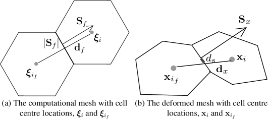
Figure 2: Cells $i$ and $i_{f}$ of the computational and deformed meshes either side of face $f$, face area vector $\mathbf{S}_{f}$ and vector between cell centres, $\mathbf{d}_{f}$. The skewness of face $f$ of the deformed mesh (b) is shown by a short grey line of length $d_{s}$ in the plane of the face (see section 5).

4.2.2 Discretisation of the Hessian

Two approaches are taken to calculate the Hessian. The first we define a finite-difference approach (which uses both finite volume and finite difference approximations). The second uses the fact that, in solving the Monge-Ampère equation for mesh generation, we are approximating the change in cell volume by the determinant of the Hessian. Therefore, rather than calculating a discretised Hessian, we can simply use the change in cell volume, $r$. This is the geometric approach. The geometric approach is always used on the surface of the sphere.

4.2.2.1 Finite Difference Discretisation of the Hessian

For a discretisation of the Hessian consistent with the discretisation of the Laplacian, we use Gauss’s theorem:

$$H\left(\phi\right)_{i}=\nabla\nabla_{i}\phi=\frac{1}{V_{i}}\sum_{f\in i}\nabla_{f}\phi\mathbf{S}_{f}$$ (26)

where $\nabla_{f}\phi$ is the vector gradient of $\phi$ located at face $f$ of cell $i$. The vector gradient, $\nabla_{f}\phi$, is reconstructed from normal components, $\nabla_{nf}\phi$ using a least-squares fit which is derived by assuming that $\nabla\phi$ is uniform so that it is first-order accurate on non-uniform meshes. This approach starts by reconstructing a cell-centred gradient from surrounding normal gradients using a least squares fit:

$$\nabla_{i}\phi=\left(\sum_{f\in i}\hat{\mathbf{S}}_{f}\mathbf{S}_{f}^{T}\right)^{-1}\sum_{f\in i}\nabla_{nf}\phi\ \mathbf{S}_{f}.$$ (27)

where $\hat{\mathbf{S}}_{f}=\mathbf{S}_{f}/|\mathbf{S}_{f}|$. Next, a temporary value of the vector valued gradient at each face is calculated:

$$\nabla_{f}^{\prime}\phi=\lambda_{f}\nabla_{i}\phi+\left(1-\lambda_{f}\right)\nabla_{i_{f}}\phi$$ (28)

where $\lambda_{f}$ is the coefficient for linear interpolation. For consistency with the Laplacian, we must have $\nabla_{f}\phi\cdot\mathbf{S_{f}}=\nabla_{nf}\phi|\mathbf{S}_{f}|$ which can be enforced with an explicit correction:

$$\nabla_{f}\phi=\nabla_{f}^{\prime}\phi+\left(\nabla_{nf}\phi-\nabla_{f}^{\prime}\phi\cdot\hat{\mathbf{S}}_{f}\right)\hat{\mathbf{S}}_{f}.$$ (29)

The Hessian calculated using eqn. (26) is not symmetric, as the analytic version would be.

4.2.2.2 Geometric approach to calculating the Hessian

A numerical approximation for calculating $H$ will introduce truncation errors so instead we can simply use the change in cell volume:

$$r_{i}=|I+H_{i}\left(\phi\right)|=\frac{V_{i}\left(\mathbf{x}\right)}{V_{i}\left(\bm{\xi}\right)}$$ (30)

where $V_{i}\left(\mathbf{x}\right)$ is the volume of the transported mesh cell $i$ and $V_{i}\left(\bm{\xi}\right)$ is the volume of the original cell. Volumes are calculated on the surface of the sphere by decomposing every polyhedron (on the original and new meshes) into tetrahedra with curved surfaces which are flat in spherical geometry. The volumes of these tetrahedra are found using the formula for the area of a spherical triangle.

4.2.3 The Gradient at the Vertices

In order to calculate the mesh map and consequently to calculate $m$, we must calculate $\nabla\phi$ at the mesh vertices, $\nabla_{v}\phi$. (This is in contrast to 19, 34 who discretise the gradient of $\phi$ at the same locations where $\phi$ is stored.) Ideally, the calculation of $\nabla_{v}\phi$ should not produce any non-convex cells and it turns out to be particularly sensitive to the numerical approximation and its stencil. In section 4.2.3.1 we will describe a large stencil gradient, for which grid-scale oscillations in $\phi$ can grow which are not seen in $\nabla_{v}\phi$ and convergence is slow. In section 4.2.3.2 we will describe a small stencil gradient which can lead to grid-scale oscillations of $\nabla_{v}\phi$ on a hexagonal mesh since the calculation of the gradient does not lead to a gradient with bounded variation. This leads to locally distorted meshes. Section 4.2.3.3 describes a compromise; a new Goldilocks stencil that combines the advantages of both large and small.

4.2.3.1 Vertex Gradient using a Large Stencil

In order to calculate $\nabla_{v}\phi$ at the vertices, $\nabla_{f}\phi$ at the faces is calculated using eqn. (29). These values are then interpolated onto the vertices using linear interpolation. On a mesh of squares, four values of $\nabla_{f}\phi$ are averaged to calculate each $\nabla_{v}\phi$ at a vertex and on a mesh of hexagons, three values of $\nabla_{f}\phi$ are averaged to calculate each $\nabla_{v}\phi$. Including the calculation of $\nabla_{f}\phi$, the reconstruction of $\nabla_{v}\phi$ from $\phi$ uses a stencil of 10 hexagons on a hexagonal mesh and 12 squares on a mesh of squares. Due to these large stencils, the gradients calculated are smooth even if the $\phi$ field is not smooth. Due to the averaging (interpolation) of the gradient from the cell centres to the vertices there will be some consistency between gradients at different vertices and so cells may remain convex.

4.2.3.2 Vertex Gradient using a Small Stencil

The vector gradient at each vertex, $\nabla_{v}\phi$, can be reconstructed directly from the normal component of the gradient at the surrounding faces using a least squares fit

$$\nabla_{v}\phi=\left(\sum_{f\in v}\mathbf{d}_{f}\mathbf{d}_{f}^{T}\right)^{-1}\sum_{f\in v}\left(\mathbf{d}_{f}\nabla_{nf}\phi\right)$$ (31)

where $f\in v$ is the set of faces which share vertex $v$. This approximation is exact for a uniform vector field, $\nabla\phi$, and is consequently first order accurate on an arbitrary mesh. However on a hexagonal mesh, eqn. (31) only uses information from three surrounding faces and three surrounding hexagons and the resulting gradients are prone to grid-scale oscillations which can lead to the creation of non-convex cells. The small amount of information used at every vertex means that neighbouring vertices can have very different gradients. We therefore need a larger stencil, but not as large as the stencil used in section 4.2.3.1.

On a mesh of squares, $\phi$ at four squares is sufficient to reconstruct a smooth $\nabla_{v}\phi$ to second order.

4.2.3.3 Vertex Gradient using the Goldilocks Stencil

The Goldilocks stencil should be large enough to calculate a smooth gradient (with bounded variation) but without including averaging which can hide grid-scale oscillations in $\phi$. The stencil used includes the faces which share vertex $v$ and the face neighbours attached by a vertex to those faces (fig. 3). The vertex gradient is then reconstructed using a least squares fit:

$$\nabla_{v}\phi=\left(\sum_{f\in v^{\prime}\in f^{\prime}\in v}\mathbf{d}_{f}\mathbf{d}_{f}^{T}\right)^{-1}\sum_{f\in v^{\prime}\in f^{\prime}\in v}\left(\mathbf{d}_{f}\nabla_{nf}\phi\right)$$ (32)

where $f\in v^{\prime}\in f^{\prime}\in v$ is the set of faces shown by dashed lines in fig. 3. In the least squares fit in eqn. (32), the central faces are counted three times (making the fit more accurate near the centre, following Weller et al. [41]).

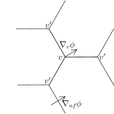
Figure 3: The Goldilocks stencil for recontructing the full gradient of the mesh potential, $\nabla_{v}\phi$, at the central vertex, $v$, from the component of the normal gradient at each face, $\nabla_{nf}\phi$. This results in a stencil of six hexagons to calculate $\nabla_{v}\phi$ at a vertex.

4.2.4 Calculation of Exponential Maps

Exponential maps are used to move vertices on the surface of the sphere. The direction of the map is given by the direction of $\nabla_{v}\phi$ at vertex $v$ (ie the direction is along the great circle in the plane of $\nabla_{v}\phi$) The distance moved is the geodesic distance $|\nabla_{v}\phi|$ so that the vertex is rotated around the sphere by an angle $|\nabla_{v}\phi|/a$ where $a$ is the radius of the sphere.

4.2.5 Linear equation solver and fixed point iterations

Spatial discretisation of eqns (21),(22) leads to a set of linear algebraic equations, which can be written as a matrix equation, $A\bm{\phi}^{(n+1)}=\mathbf{b}^{(n)}$, where $\bm{\phi}^{(n+1)}$ is the vector of all of the values of the unknown, $\phi^{(n+1)}$. This matrix equation is solved using the OpenFOAM GAMG solver (geometric algebraic multi-grid, [32]) using diagonal incomplete Cholesky smoothing with 50 cells in the coarsest level. The residual for the solver tolerance is defined as:

$$\frac{\sum|\mathbf{b}-A\bm{\phi}|}{\sum\left(|\mathbf{b}|+|A\mathbf{\bm{\phi}}|\right)}$$ (33)

where the sum is over all cells of the mesh (ie over all elements of the vectors $\mathbf{b}$ and $A\bm{\phi}$). For each fixed-point iteration, the values of $\phi$ from the previous iteration are used as an initial guess for the solution of the matrix equation, so the initial residual should converge to the final residual as the fixed-point iterations converge. At each fixed point iteration (ie each value of $n$ in eqn. (21)) the matrix equation is solved with a tolerance equal to the maximum of 0.001 times the initial residual and $10^{-8}$. The matrix equation is not solved all the way to $10^{-8}$ at every fixed-point iteration to save computational cost but, when the fixed-point iterations have converged, the initial residual will be less than $10^{-8}$. A weaker tolerance is probably acceptable for mesh generation but we are using a tight tolerance to have more confidence that the numerical method is convergent.

4.2.6 Moving Voronoi Generating Points

If the initial mesh is Voronoi and it is required that the transported mesh is also Voronoi, then the Voronoi generating points can be moved using eqn. (2) using the cell centre gradient, reconstructed from the face gradient using volume weighting. Then the moved generating points can be re-tesselated to create a new Voronoi tesselation. However, the re-tesselation may not have exactly the same connectivity due to edge swapping in the Delaunay algorithm. This technique therefore may not be so suitable for r-adaptivity.

4.2.7 Calculating the Monitor Function

When using r-adaptivity, the mesh monitor function (that controls the mesh density) will need to be mapped from the previous mesh onto the new transported mesh so that it can be evaluated when solving eqns. (21) or (22). In section 6, we first present results using an analytic monitor function, which is evaluated at the transported mesh cell centres. We then use observed meteorological data to calculate a monitor function by mapping the data to the computational grid and then apply Laplacian smoothing, as described in section 4.3.2.

4.3 Enforcing Stability

4.3.1 Under-relaxation

Here we describe how $\alpha$ is calculated. We start by defining the source terms of the eqns (21),(22) to be $s^{n}=|I+H\left(\phi^{n}\right)|-c/m({\bf x}^{n})$ and $s^{n}=r\left(\phi^{n}\right)-c/m({\bf x}^{n})$ respectively. For convergence to occur, we would like the source term to decrease relative to the Laplacian term, $\nabla^{2}\phi$. Initially, the source term has order 1. In the tests undertaken, both on the plane and on a sphere, it has been sufficient to keep the ratio of the Laplacian to the source term greater than four and to always ensure that $\alpha$ increases with iteration number, $n$. So $\alpha$ is set to be:

$$1+\alpha^{n+1}=\max\left(1+\alpha^{n},\ 4\max\left({}^{1}\!\!/\!_{4},\ \max\left(|s^{n}|\right)\right)\right)$$ (34)

4.3.2 Smoothing the Monitor Function

Following Browne et al. [5], we experimented with smoothing the monitor function and this smoothing certainly improved convergence and generated meshes with smoother grading and hence lower anisotropy and skewness and better orthogonality (see section 5). However the purpose of this work is to describe a robust solution of the Monge-Ampère equation on the sphere for any monitor function. So smoothing of the monitor function will not be considered for the analytically defined monitor functions. However, when using meteorological data to define a monitor function, the monitor function is smoothed on the computational grid during each iteration using Laplacian smoothing:

$$m = m^{\prime}\left(\exp_{\xi}\nabla\phi\right)+\frac{1}{4}\nabla\cdot\left(|\mathbf{d}_{f}|^{2}\nabla m^{\prime}\left(\exp_{\xi}\nabla\phi\right)\right)$$

where $m^{\prime}$ is the monitor function mapped from the meteorological data onto the physical grid at position $\exp_{\xi}\nabla\phi$ and $m$ is the monitor function used in the source terms of eqns. (21),(22). The diffusion coefficient used is the square of the mesh spacing, $|\mathbf{d}_{f}|$ on the computational grid.

5 Diagnostics of Convergence and of Mesh Quality

Convergence is measured in two ways. Firstly, convergence is measured by plotting the initial residual (eqn 33) of the matrix equation at every fixed point iteration as a function of iteration number. This gives an indication of how much the solution is changing for each fixed-point iteration.

Secondly, the convergence of the final solution is assessed by plotting the change in cell area between the initial mesh and the final iteration for every cell in comparison to $c/m$. At convergence, these should be equal. The test cases considered use an axi-symmetric monitor function, $m$, so this measure is plotted as a scatter plot against distance to the axis of symmetry. This tells us where the solution is not converging to the required monitor function and also, for solutions using $|I+H\left(\phi^{n}\right)|$ instead of $r\left(\phi^{n}\right)$ (ie using the finite difference Hessian rather than the geometric Hessian) in the Monge-Ampère equation, it tells us how well $|I+H\left(\phi^{n}\right)|$ approximates $r\left(\phi^{n}\right)$.

The diagnostics of mesh quality consider cell centres, defined as cell centroids or centres of mass of the moved cells, and face centres, defined in the same way. These will also use the face area vector, $\mathbf{S}_{x}$, the normal vector to each face with magnitude equal to the face area and $\mathbf{d}_{x}$, the vector between cell centres either side of a face of the deformed mesh (see fig 2(b)).

In order to measure mesh quality, firstly we will consider mesh spacing, $|\mathbf{d}_{x}|$, between adjacent cell centres for each cell face as a scatter diagram as a function of distance to the axis of symmetry (for the axi-symmetric cases). This informs us about the aspect ratios of the cells since cells with high aspect ratio will give a large scatter of values of $|\mathbf{d}_{x}|$ for a given distance to the axis of symmetry. If the mesh is perfectly equidistributed then cell areas should be given by $c/m$. Therefore, for the meshes of quadrilaterals, $|\mathbf{d}_{x}|$ will be compared with $\sqrt{c/m}$ and for the meshes of mostly hexagons, $|\mathbf{d}_{x}|$ will be compared with $\sqrt{2c\ \tan(\pi/3)/3m}$ .

The second mesh quality diagnostic is non-orthogonality for each cell face which is measured as

$$\text{non-orthogonality}=\cos^{-1}\frac{\mathbf{S}_{x}\cdot\mathbf{d}_{x}}{|\mathbf{S}_{x}||\mathbf{d}_{x}|}.$$ (35)

The third mesh quality diagnostic is the face skewness, measured as the distance, $d_{s}$, between the face centre and the crossing point between the vector $\mathbf{d}_{x}$ with the face, normalised by $|\mathbf{d}_{x}|$:

$$\text{skewness}=\frac{d_{s}}{|\mathbf{d}_{x}|}.$$ (36)

The skewness distance, $d_{s}$, is shown as a short grey line in fig. 2(b). This definition of skewness is a feature of the non-linearities of the map generating the mesh and is different quantitatively and qualitatively from that of Budd et al. [9] which can be calculated directly the Jacobian of the map. The skewness metric, $Q$, from Budd et al. [9] gives information about isotropy and orthogonality, not face skewness.

6 Results

Optimally transported meshes are generated in two-dimensional planar geometry to compare with those generated by numerical solution of the parabolic Monge-Ampère equation by Budd et al. [9]. Next, OT meshes are generated on the surface of the sphere in order to compare with the centroidal Voronoi meshes generated by Ringler et al. [33] using Lloyd’s algorithm. Finally, OT meshes are generated on the sphere using observed precipitation to define a monitor function.

6.1 Optimally Transported Meshes in Euclidean Geometry

Meshes are generated on a finite plane, $[-1,1]^{2}$, using the radially symmetric monitor function used by Budd et al. [9] defined for each location $\mathbf{x}_{i}$:

$$m\left(\mathbf{x}_{i}\right)=1+\alpha_{1}\text{sech}^{2}\left(\alpha_{2}\left(R^{2}-a^{2}\right)\right)$$ (37)

where $\mathbf{x}_{c}$ is the centre of the refined region (the origin for these results), $R$ is the distance of $\mathbf{x}_{i}$ to $\mathbf{x}_{c}$ and $\alpha_{1}$, $\alpha_{2}$ and $a$ control the variations of the density function. Following Budd et al. [9] we generate two types of mesh with this monitor function, the first we call the ring mesh using $a=0.25$, $\alpha_{1}=10$ and $\alpha_{2}=200$ and the second the bell mesh using $a=0$, $\alpha_{1}=50$ and $\alpha_{2}=100$, both using periodic boundary conditions for $\phi$. The computational meshes on which the optimal transport problems are solved are uniform grids of $60\times 60$ squares.

The ring and bell meshes generated using both the finite difference and the geometric Hessian on the plane are shown in figure 4. The convergence diagnostics will be presented in section 6.2. Mesh quality for these meshes was analysed by Budd et al. [9] and this is not repeated here.

Figure 4: A quarter of the ring and bell meshes using the finite difference and volume Hesssian.

The meshes in fig. 4 calculated using both Hessian techniques are similar to each other and they are also similar to the meshes generated by Budd et al. [9].

6.2 Convergence of the Monge-Ampère Solution in Euclidean Geometry

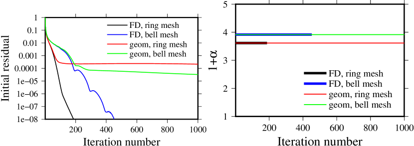
Figure 5: Convergence of initial residual of the solution of the Poisson equation for each fixed point iteration and $1+\alpha$ as a function of iteration number for the planar meshes generated with the monitor function defined in eqn. (37).

Figure 5 on the left shows the initial residual of the matrix solution as a function of iteration number for the calculation of all of the meshes on the plane. Using the finite difference Hessian, the solution converges rapidly but convergence stalls when using the geometric Hessian. There are two possible reasons for the stalling. Firstly, the Laplacian is no longer a good linearisation of the geometric Hessian and secondly, a solution at this resolution may not exist. Smoothing the monitor function removes the stall in convergence and speeds convergence of all solutions (not shown) since smoothing removes the very abrupt changes in the monitor function. However this is not the topic of this paper.

The underelaxation factor, $1+\alpha$, is shown in the right of fig. 5. It never rises above the initial value because the source term never increases above its initial value. The initial value of $1+\alpha$ is simply $4\max|1-c/m|$ and so $1+\alpha$ is independent of the Hessian calculation method.

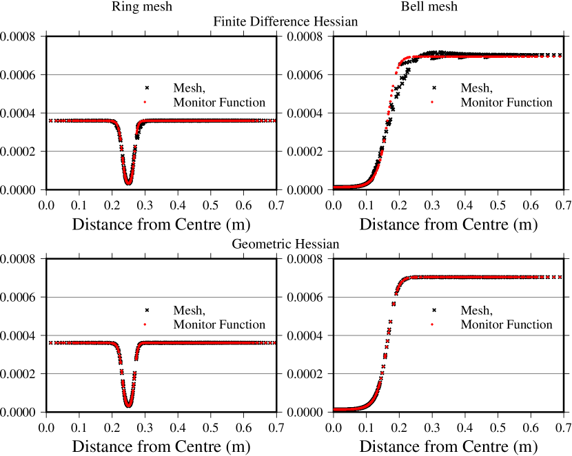
Figure 6: Cell area as a function of distance from the axis of symmetry in comparison to that implied by the monitor function ($c/m$) for the planar meshes generated with the monitor function defined in eqn. (37).

In order to diagnose how closely the final mesh equidistributes the monitor function, we plot the cell area as a scatter plot for every cell in the mesh as a function of the distance from the axis of symmetry in fig. 6 in comparison with $c/m$. Using the finite difference Hessian, there are discrepancies between $c/m$ and the cell area where the second derivative of $c/m$ is high. This is because the discrete calculation of the Hessian is not a good approximation of the cell area in these regions, where the derivatives of $\phi$ are varying rapidly. However, for the purpose of mesh generation, these discrepancies do not look problematic. If the OT mesh is smoother than that specified by the monitor function then it could be beneficial. The meshes generated using the geometric Hessian are more accurately equidistributed with respect to the monitor function, despite the lack of convergence of the initial residual.

6.3 Optimally transported and Centroidal Voronoi meshes on the Sphere

Meshes are generated using the geometric Hessian in order to compare with the locally refined centroidal Voronoi meshes generated using Lloyd’s algorithm by Ringler et al. [33]. We use a monitor function given by the square root of the density function of the corrected eqn. (4) of Ringler et al. [33]:

$$m\left(\mathbf{x}_{i}\right)=\sqrt{\frac{1}{2\left(1+\gamma\right)}\left(\tanh\frac{\beta-||\mathbf{x}_{c}-\mathbf{x}_{i}||}{\alpha}+1\right)+\gamma}$$ (38)

where $\mathbf{x}_{c}$ is the centre of the refined region which has a latitude of $30^{o}$ and a longitude of $90^{o}$. $||\mathbf{x}_{c}-\mathbf{x}_{i}||$ is the geodesic distance between the points and is computed as $\cos^{-1}\left(\mathbf{x}_{c}\cdot\mathbf{x}_{i}\right)$. $\alpha$ and $\beta$ are in radians and they control the size of the refined region and the distance over which the mesh changes from fine to coarse resolution. We follow Ringler et al. [33] and use $\alpha=\pi/20$ and $\beta=\pi/6$. $\gamma$ controls the ratio between the finest and coarsest resolution and we use $\gamma=\left(1/2\right)^{4}$, $\gamma=(1/4)^{4}$, $\gamma=(1/8)^{4}$ and $\gamma=(1/16)^{4}$ for meshes with finest mesh spacing factors of 2, 4, 8 and 16 times smaller than that of the coarsest. Following Ringler et al. [33], these meshes are referred to as X2, X4, X8 and X16.

The computational meshes are hexagonal icosahedra which consist of 12 pentagons and $10(2^{2n}-1)$ hexagons for $n=3,4,5,6$. These quasi-uniform meshes can be referred to as the X1 meshes. The X1 meshes are not shown but the X1 centroidal Voronoi meshes and the OT meshes are slightly different. The X1 centroidal Voronoi meshes are generated using Lloyd’s algorithm which guarantees that the X1 meshes are nearly centroidal (the Voronoi generating point is co-located with the cell centre) whereas the X1 OT meshes are the Heikes and Randall [23] version of the hexagonal icosahedron, optimised to reduce face skewness. The X2, X4, X8 and X16 meshes of 2,562 cells are shown in figure 7 with the ratio between the cell area and the average cell area coloured.

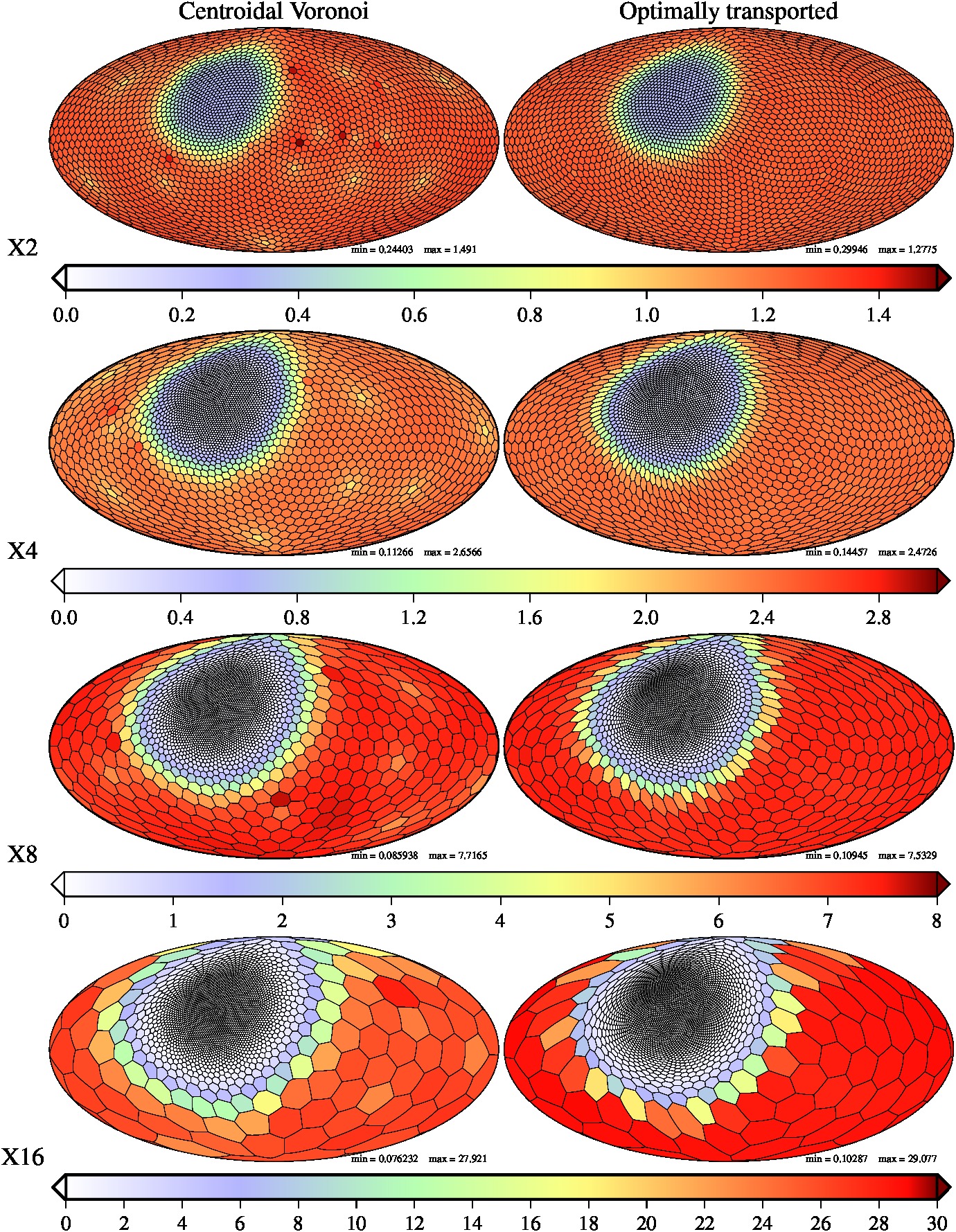
Figure 7: X2, X4, X8 and X16 meshes of the sphere of 2,562 cells and the cell volumes relative to the average cell volume in colour. The surface of the entire sphere is displayed using a Hammer equal-area projection [42].

The centroidal Voronoi meshes in fig. 7 are orthogonal, close to centroidal and the mesh topology (connectivity) is different for all the refinement levels. (Lloyd’s algorithm generates meshes that are centroidal relative to a density function which means that they are not centroidal when the centroid is simply the centre of mass.) The OT meshes all have the same connectivity and they are centroidal but not orthogonal. (Orthogonality could be achieved by Voronoi tesselating the meshes, at the expense of centroidality, see section 6.6.)

All of the OT meshes in fig. 7 have regions of anisotropy in between the fine and coarse regions whereas the centroidal Voronoi meshes remain isotropic and the mesh topology changes between resolutions. The anisotropy will be investigated further in section 6.5. Before looking in more detail at the mesh quality in section 6.5, we will examine diagnostics of convergence in section 6.4.

6.4 Convergence of the Monge-Ampère Solution on the Sphere

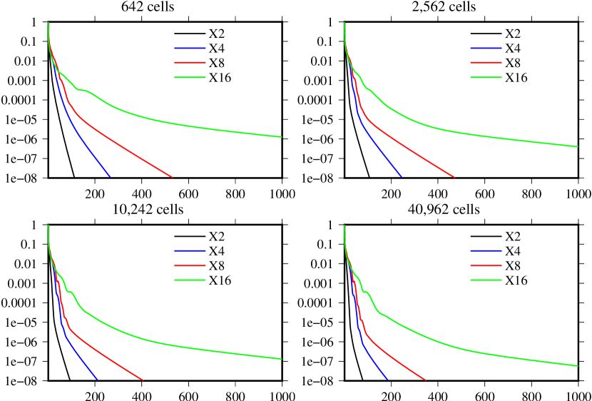
Figure 8: Convergence of initial residuals with iteration number for all of the optimally transported meshes on the sphere

Convergence of the initial residual is shown in fig. 8 for the X2-X16 meshes of various resolutions. Convergence is rapid for the X2 and X4 meshes but slows after around 100 iterations, once the non-linearities have grown and the Laplacian is no longer a good approximation for the Hessian and once the exact solutions becomes difficult to achieve at finite resolution. It appears from fig. 8 that the number of iterations reduces as mesh size increases.

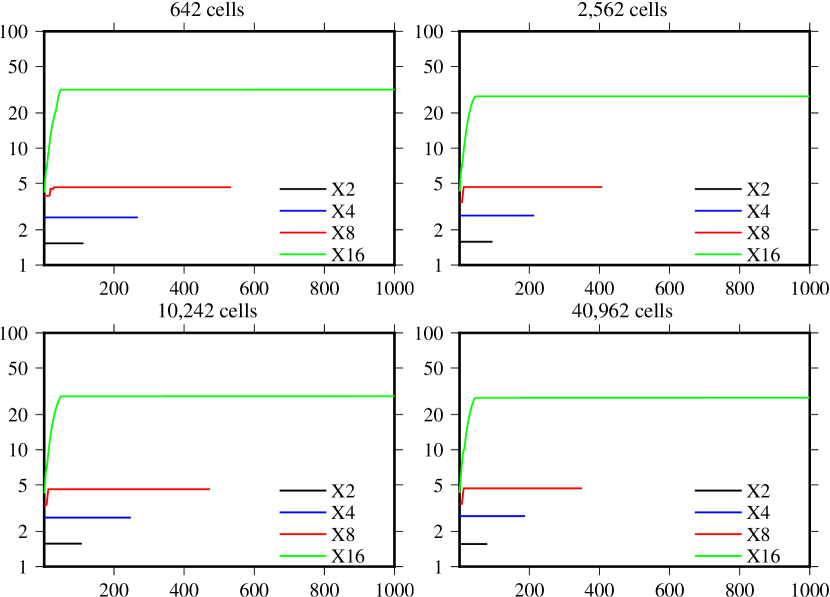
Figure 9: Under-relaxation factor, $1+\alpha$, for with iteration number for all of the optimally transported meshes on the sphere

The underelaxation factor, $1+\alpha$, is shown in fig. 9. Unlike in the Euclidean case, $1+\alpha$ does rise after initialisation. This implies that the maximum of the source term increases before it decreases. However the initial residual is monotonically decreasing during these early iterations. This is because the initial residual is a mean over the whole domain whereas $1+\alpha$ is set from the maximum of the source term.

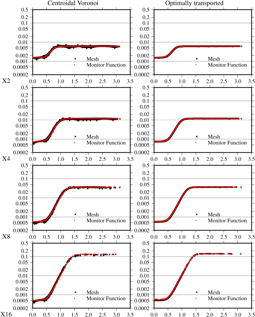
Figure 10: Cell area as a function of geodesic distance to the centre of the refined region in comparison to that implied by the monitor function ($c/m$) for the X2, X4, X8 and X16 meshes of 2,562 cells

The convergence of the cell area with the monitor function is shown in fig. 10 as scatter plots of cell area change as a function of distance to the centre of the refined region. As occurred in Euclidean geometry, the geometric Hessian gives accurate equidistribution.

6.5 Mesh Quality on the Sphere

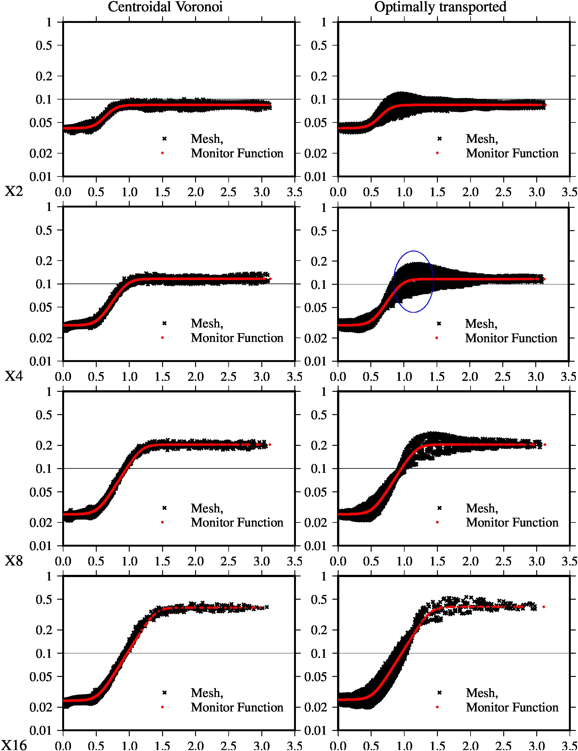
Figure 11: Cell-centre to cell-centre geodesic distance ($|\mathbf{d}_{x}|$ as defined in section 5) as a function of geodesic distance to the centre of the refined region in comparison to that implied by the monitor function ($\sqrt{2c\ \tan(\pi/3)/3m}$) for the X2, X4, X8 and X16 meshes of 2,562 cells. The blue encircled region for X4 shows where the OT mesh is anisotropic.

Scatter plots of the cell-centre to cell-centre distance, $|\mathbf{d}_{x}|$, as a function of distance to the centre of the refined region are shown in fig. 11 for the X2-X16 meshes of 2,562 cells on the sphere. This shows that the centroidal Voronoi meshes are close to isotropic whereas the OT meshes have high anisotropy where the second derivative of the monitor function is high. In particular, a region of anisotropy is indicated by a blue ring for the X4 OT mesh in fig. 11: there is a wide range of $|\mathbf{d}_{x}|$ at the same distance to the centre of the refined region, indicating anisotropy. This anisotropy could be reduced by smoothing the monitor function.

Unlike the meshes on the plane, the meshes on the sphere are isotropic in the uniformly coarse region, due to the isotropy of the domain relative to the centre of refinement. This could be an advantage of using r-adaptivity on the sphere over its use in Euclidean geometry with corners. However the meshes on the sphere still have a bulge in $|\mathbf{d}_{f}|$ on the edge of the coarse region. This is not ideal for atmospheric simulations since global errors are often proportional to the largest $|\mathbf{d}_{x}|$ [33].

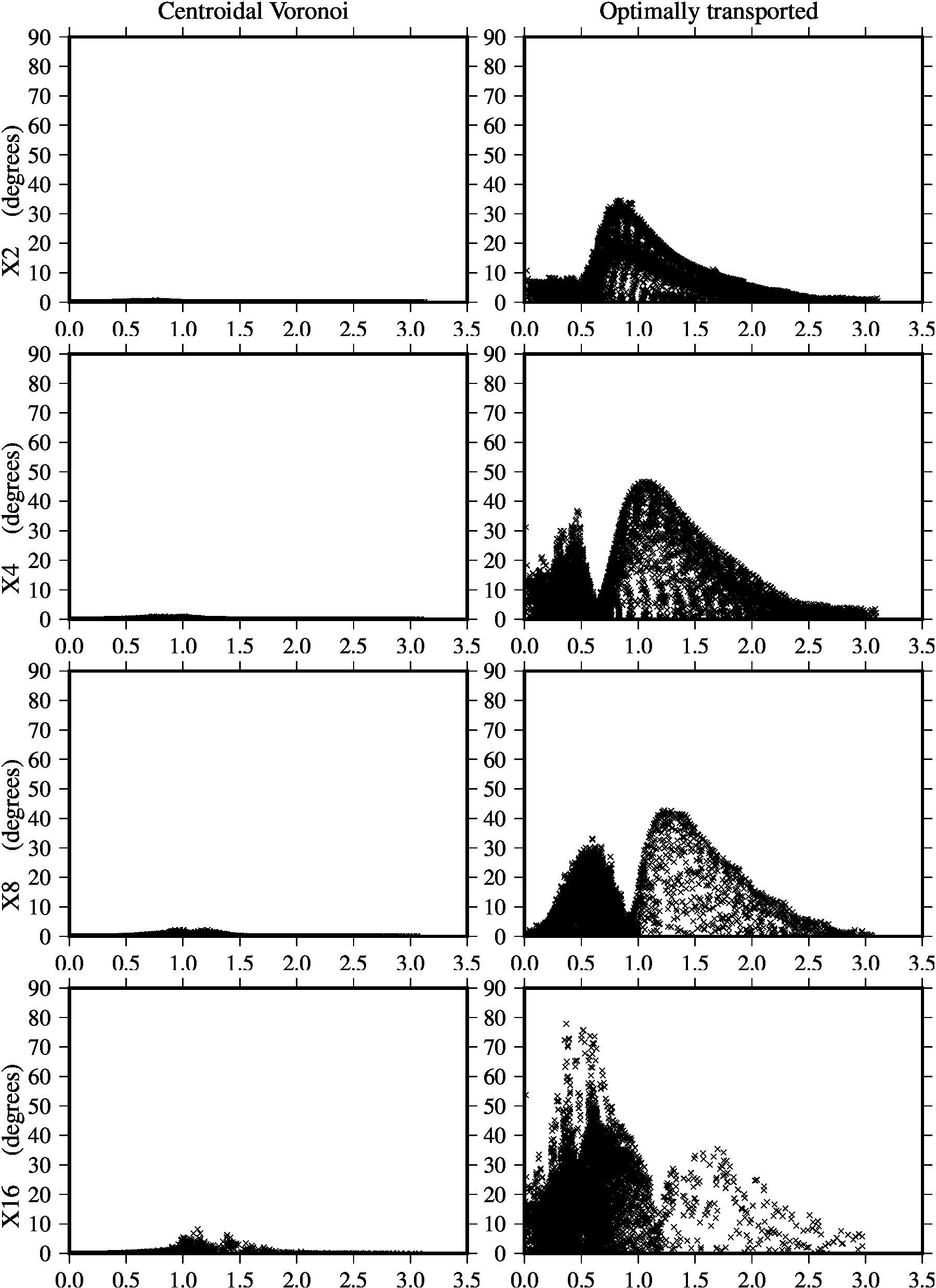
Figure 12: Non-orthogonality of the meshes on the sphere (as defined in eqn. 35) as a function of geodesic distance to the centre of the refined region for the X2-X16 meshes of 2,562 cells

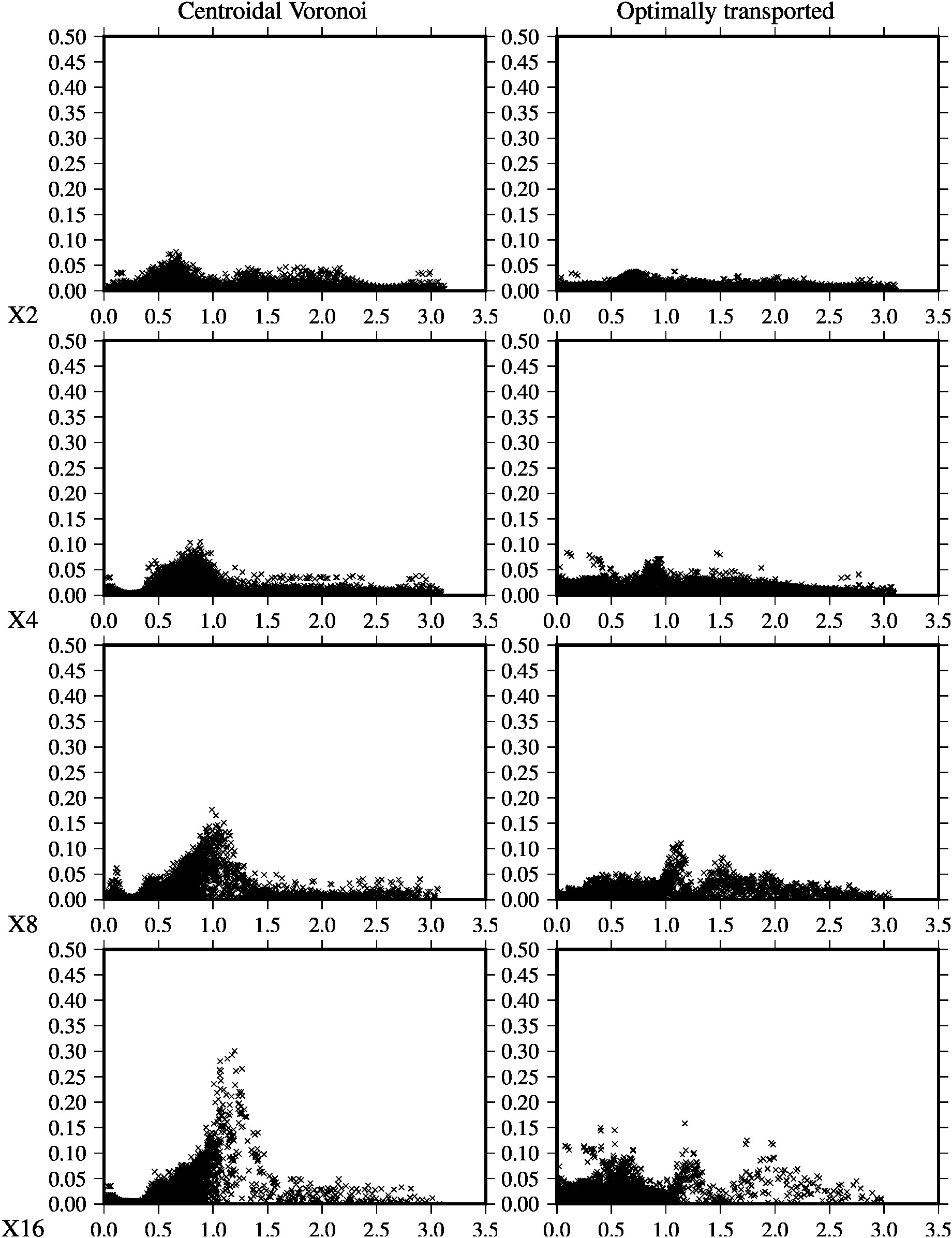
Figure 13: Face skewness ($d_{s}/|\mathbf{d}_{x}|$, as defined in eqn. 36) as a function of geodesic distance to the centre of the refined region for the X2 and X4 meshes of 2,562 cells

The orthogonality and skewness of the faces of the OT X2-X16 meshes on the sphere are shown in figs. 12 and 13 in comparison to the centroidal Voronoi meshes. Lloyd’s algorithm with a non-uniform monitor function generates exactly orthogonal, non-centroidal meshes and so for comparison with the OT meshes, the Voronoi meshes are made exactly centroidal at the expense of orthogonality by using the cell centroid as the cell centre rather than using the Voronoi generating point. Even so, they remain very close to orthogonal in comparison to the OT meshes which have high non-orthogonality where the second derivative of the monitor function is high (for this test case). In fact the non-orthogonality reaches over 70 degrees for some cells in the X16 mesh. This is unlikely to be a good mesh for simulation. This problem will be investigated further in section 6.6.

The OT meshes have less face skewness, $d_{s}/|\mathbf{d}_{x}|$, than the centroidal Voronoi meshes (fig 13) which could be advantageous for numerical methods whose errors depend on skewness. For example, Heikes and Randall [23] described how to optimise orthogonal meshes to reduce skewness for low-order finite-volume discritisations.

6.6 Improving Convexity

The OT X16 meshes presented in sections 6.3-6.5 have some large non-orthogonality at regions where the resolution is changing rapidly (fig 12). The reason for this can be seen more clearly in a zoomed regions of the meshes in the second row of fig. 14. The double zoomed plot shows that some of the cells are not convex. This implies that the calculation of $\nabla_{v}\phi$ has in fact not yielded a smooth vector field, despite the development of the Goldilocks stencil with the aim of achieving a smooth $\nabla_{v}\phi$ on the smallest possible stencil. The Goldilocks stencil does give a much smoother $\nabla_{v}\phi$ than the small stencil (first row of fig 14). If instead we interpolate $\nabla\phi$ from faces onto vertices which entails the use of the larger stencil (secn 4.2.3.1), the non-convex cells are not generated (third row of fig 14). Alternatively, a Voronoi tessellation can be created using the cell centres of the Goldilocks stencil mesh as generating points (bottom row of fig. 14). This also eliminates non-convex cells.

Figure 14: Zoomed and double zoomed X16 meshes with 2,562 cells using different calculations of $\nabla_{v}\phi$ and Voronoi versions.

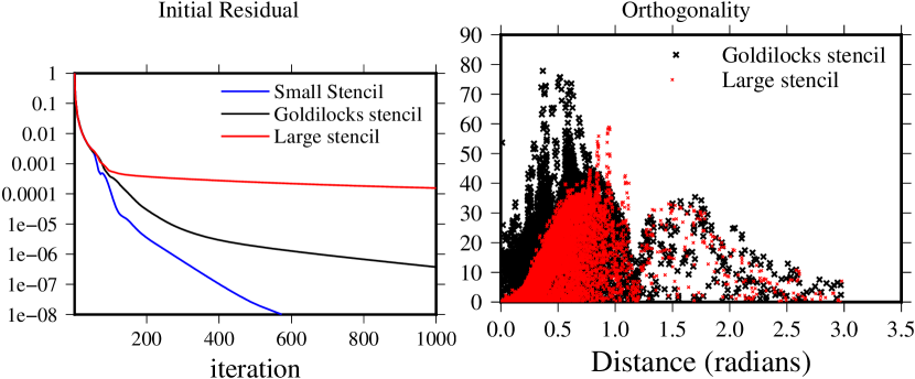
Figure 15: Comparisons of convergence of initial residuals and orthogonality for the X16 meshes of 2,562 cells calculated using the geometric Hessian but with different calculations of $\nabla_{v}\phi$.

The problem with the large stencil calculation of $\nabla_{v}\phi$ is that convergence is slowed and orthogonality is only reduced a little (fig 15). Therefore it is necessary to consider the Voronoi tessellation of the cell centres (final row of fig. 14). This modification does not affect the convergence since the Voronoi tessellation is calculated after convergence of the Monge-Ampère solution. This mesh is insensitive to the calculation of $\nabla_{v}\phi$ but is no longer exactly equidistributed because the cell areas change a little (locally) when the Voronoi tesselation is calculated (fig 16). However these area changes are very small and simply smooth out the curve where the monitor function flattens out into the coarse region. Fig 16 also shows that the Voronoi version is more orthogonal than the large stencil version, the anisotropy is similar and the skewness is increased. However, the connectivity may be changed slightly.

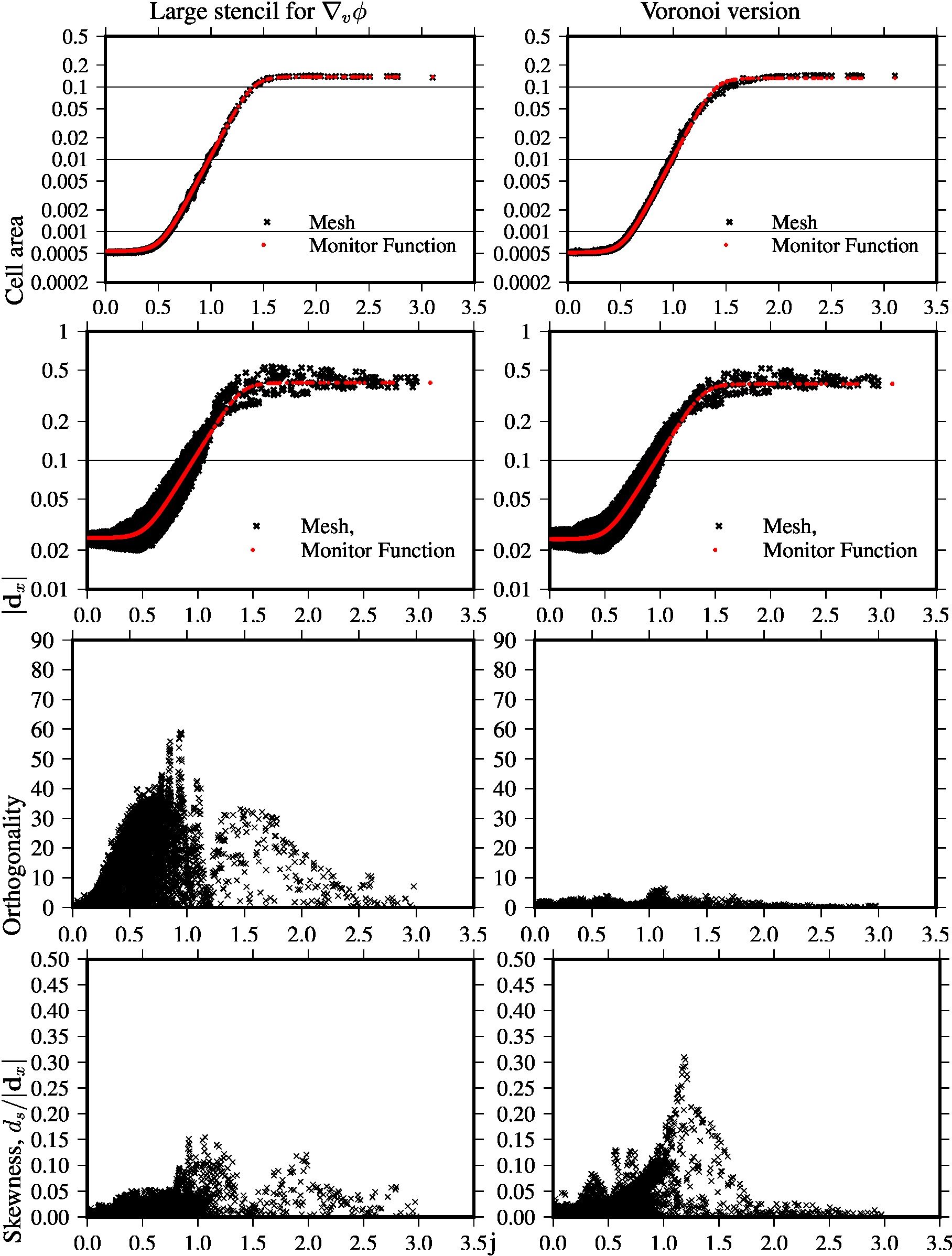
Figure 16: Mesh diagnostics as a function of distance from the centre of the refined region for the X16 meshes of 2,562 cells using the large stencil for $\nabla_{v}\phi$ on the left and using the Voronoi tesselation on the right.

6.7 Optimally Transported Meshes using Precipitation as a Monitor Function

In order to demonstrate the numerical solution of the Monge-Ampère type equation using realistic data as a monitor function, meshes are generated based on the daily average precipitation rate from the NOAA-CIRES 20th Century Reanalysis version 2 (10, http://www.esrl.noaa.gov/psd/data/gridded/data.20thC_ReanV2.html) on 9 Oct 2012. The numerical solution of the Monge-Ampère equation uses two near uniform hexagonal-icosahedral meshes of 2,562 and 10,242 cells. The re-analysis precipitation ranges from zero to $p_{\max}=8.73\times 10^{-4}\text{kg}\text{m}^{-2}\text{s}^{-1}$. A strictly positive, non-dimensional monitor function, $m$, is defined from the precipitation rate, $p$ using:

$$m=\frac{p+p_{\min}}{p_{\max}+p_{min}}$$ (39)

where the minimum allowable values is set to $p_{\min}=10^{-5}\text{kg}\text{m}^{-2}\text{s}^{-1}$. The resulting meshes are shown in fig. 17 (and are highly sensitive to the value of $p_{\min}$ used). Precipitation clearly could not be used as a monitor function for a dynamically adapting simulation of the global atmosphere since it is strongly resolution dependent. Instead, monitor functions with less resolution dependency should be developed. Reanalysis precipitation is used here just as a demonstration of the solution when using realistic meteorological data.

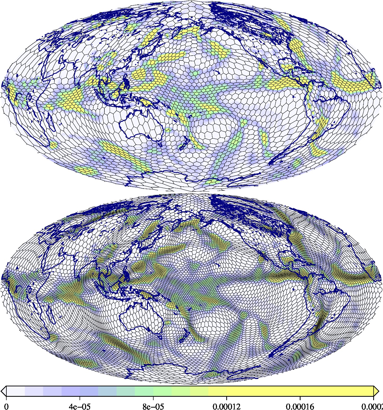
Figure 17: Meshes of 2,562 and 10,242 cells generated based on the monitor function of precipitation on 9 Oct 2012. The colours show the precipitation rate in $\text{kg}\text{m}^{-2}\text{s}^{-1}$. The surface of the entire sphere is displayed using a Hammer equal-area projection [42].

The meshes resolved based on precipitation show excellent refinement along fronts, particularly looking at South America. The Inter-tropical convergence zone is also refined in the latitudinal direction. However, based on the limitations of r-adaptivity, the Inter-tropical convergence zone cannot be refined everywhere around the equator in the longitudinal direction. If this were a requirement, a mesh starting with more points around the equator should be used. This is the subject of future research.

7 Conclusions

A technique for generating optimally transported (OT) meshes, solving a Monge-Ampère type equation on the surface of the sphere, has been developed in order to generate meshes which are equidistributed with respect to a monitor function. Equations of Monge-Ampère type have not before been solved numerically on the surface of a sphere. We show that a unique solution to the optimal mesh transport problem on the sphere exists and exponential maps are used to create the map from the old to the new mesh. We introduce a geometric interpretation of the Hessian rather than a numerical approximation which is accurate on the surface of the sphere. In order to create a semi-implicit algorithm, a new linearisation of the Monge-Ampère equation is proposed which includes a Laplacian term and the resulting Poisson equation is solved at each fixed-point iteration.

To validate the novel aspects of the numerical method, we first reproduce some known solutions of the Monge-Ampère equation on a two dimensional plane and find that the geometric interpretation of the Hessian leads to more accurate equidistribution than a finite difference discretisation. We also generate OT meshes of polygons on the sphere to compare with the centroidal Voronoi meshes generated by Ringler et al. [33]. The geometric Hessian created accurately equidistributed meshes on the surface of the sphere. The algorithm is found to be sensitive to the numerical method used to calculate the gradient of the mesh potential (the map to the new mesh) with a compact stencil leading to non-convexity and a large stencil leading to very slow convergence. The mesh tangling can be eliminated by creating a Voronoi tessellation of the cell centres of the final mesh. The exact solution of the OT problem on the sphere is c-convex which means that the mesh should not tangle. A numerical method which reproduces this property will be the subject of future work.

The meshes generated have advantages and disadvantages relative to centroidal Voronoi meshes generated using Lloyd’s algorithm. In principle, OT meshes should be much faster to generate, although we do not yet have timing comparisons. OT meshes do not change their connectivity with respect to the base, uniform mesh, so these meshes can be used in r-adaptive simulations. In comparison to centroidal Voronoi meshes, the OT meshes are non-orthogonal and less isotropic but have less face skewness. In order to overcome the non-orthogonality of OT meshes, the OT technique can be used to generate Voronoi meshes.

Finally, we generate a mesh using a monitor function based on reanalysis precipitation. This mesh refines smoothly along atmospheric fronts and convergence zones and provides inspiration for using r-adaptivity for global atmospheric modelling. Suitable monitor functions for r-adaptive simulations is also the subject of future work.

References

- Ahmad [2004] N. Ahmad. The Geometry of Shape Recognition via the Monge-Kantorovich Optimal Transport Problem. PhD thesis, Providence, RI, USA, 2004. AAI3134240.
- Benamou et al. [2010] J.-D. Benamou, B. Froese, and A. Oberman. Two numerical methods for the elliptic Monge-Ampére equation. ESAIM: Mathematical Modelling and Numerical Analysis, 44(4):737–758, 2010.
- Berger and Oliger [1984] M. Berger and J. Oliger. Adaptive mesh refinement for hyperbolic partial differential equations. J. Comput. Phys., 53:484–512, 1984.
- Brenier [1991] Y. Brenier. Polar Factorization and Monotone Rearrangement of Vector-Valued Functions. Communications on Pure and Applied Mathematics, XLIV:375–417, 1991.
- Browne et al. [2014] P. Browne, C. Budd, C. Piccolo, and M. Cullen. Fast three dimensional r-adaptive mesh redistribution. J. Comput. Phys., 2014.
- Budd and Williams [2006] C. Budd and J. Williams. Parabolic Monge-Ampère methods for blow-up problems in several spatial dimensions. J. Phys. A, 39(19):5425–5444, 12 May 2006.
- Budd et al. [2009] C. Budd, W. Huang, and R. Russell. Adaptivity with moving grids. Acta Numerica, 18:111–241, 2009.
- Budd et al. [2013] C. Budd, M. Cullen, and E. Walsh. Monge-Ampére based moving mesh methods for numerical weather prediction, with applications to the eady problem. J. Comput. Phys., 236(247-270), 2013.
- Budd et al. [2015] C. Budd, R. Russell, and E. Walsh. The geometry of r-adaptive meshes generated using optimal transport methods. J. Comput. Phys., 282:113–137, 2015.
- Compo et al. [2011] G. Compo, J. Whitaker, P. Sardeshmukh, N. Matsui, R. Allan, X. Yin, B. Gleason, R. Vose, G. Rutledge, P. Bessemoulin, S. Bronnimann, M. Brunet, R. Crouthamel, A. Grant, P. Groisman, P. Jones, M. Kruk, A. Kruger, G. Marshall, M. Maugeri, H. Mok, O. Nordli, T. Ross, R. Trigo, X. Wang, S. Woodruff, and S. Worley. The twentieth century reanalysis project. Quart. J. Roy. Meteor. Soc., 137:1–28, 2011.
- Cossette et al. [2014] J.-F. Cossette, P. Smolarkiewicz, and P. Charbonneau. The Monge-Ampére trajectory correction for semi-Lagrangian schemes. J. Comput. Phys., 274:208–229, 2014.
- Cotter and Shipton [2012] C. Cotter and J. Shipton. Mixed finite elements for numerical weather prediction. J. Comput. Phys., 231(21):7076–7091, Aug 2012.
- Dean and Glowinski [2006a] E. Dean and R. Glowinski. Numerical methods for fully nonlinear elliptic equations of the Monge-Ampére type. Computer methods in applied mechanics and engineering, 195(13):1344–1386, 2006a.
- Dean and Glowinski [2006b] E. Dean and R. Glowinski. An augmented Lagrangian approach to the numerical solution of the Dirichlet problem for the elliptic Monge-Ampére equation in two dimensions. Electronic Transactions on Numerical Analysis, 22:71–96, 2006b.
- Dietachmayer and Droegemeier [1992] G. Dietachmayer and K. Droegemeier. Application of continuous dynamic grid adaption techniques to meteorological modeling. Part I: Basic formulation and accuracy. Mon. Wea. Rev., 120(8):1675–1706, 1992.
- Du et al. [1999] Q. Du, V. Faber, and M. Gunzburger. Centroidal Voronoi tessellations: Applications and algorithms. SIAM Review, 41(4):637–676, 1999.
- Feng and Neilan [2009] X. Feng and M. Neilan. Mixed finite element methods for the fully nonlinear Monge-Ampére equation based on the vanishing moment method. SIAM Journal on Numerical Analysis, 47(2):1226–1250, 2009.
- Fiedler and Trapp [1993] B. Fiedler and R. J. Trapp. A fast dynamic grid adaption scheme for meteorological flows. Mon. Wea. Rev., 121(10):2879–2888, 1993.
- Froese [2012] Froese. Numerical Methods for the Elliptic Monge-Ampère Equation and Optimal Transport. PhD thesis, Simon Fraser University, 2012.
- Froese and Oberman [2011] B. Froese and A. Oberman. Convergent finite difference solvers for viscosity solutions of the elliptic Monge-Ampére equation in dimensions two and higher. SIAM Journal on Numerical Analysis, 49(4):1692–1714, 2011.
- Froese et al. [2015] B. Froese, A. Oberman, and T. Salvador. Numerical methods for the 2-Hessian elliptic partial differential equation. arXiv:1502.04969, 2015.
- Giraldo and Rosmond [2004] F. Giraldo and T. Rosmond. A scalable spectral element Eulerian atmospheric model (SEE-AM) for NWP: Dynamical core tests. Mon. Wea. Rev., 132(1):133–153, 2004.
- Heikes and Randall [1995] R. Heikes and D. Randall. Numerical integration of the shallow-water equations on a twisted icosahedral grid. Part II: A detailed description of the grid and an analysis of numerical accuracy. Mon. Wea. Rev., 123:1881–1997, June 1995.
- Huang [2001] W. Huang. Variational mesh adaption: Isotropy and equidistribution. J. Comput. Phys., 174(2):903–924, 2001.
- Jacobsen et al. [2013] D. Jacobsen, M. Gunzburger, T. Ringler, J. Burkardt, and J. Peterson. Parallel algorithms for planar and spherical Delaunay construction with an application to centroidal Voronoi tessellations. Geosci. Model Dev., 6:1353–1365, 2013.
- Kühnlein et al. [2012] C. Kühnlein, P. Smolarkiewicz, and A. Dörnbrack. Modelling atmospheric flows with adaptive moving meshes. J. Comput. Phys., 231(7):2741–2763, 2012.
- Li et al. [2001] R. Li, T. Tang, and P. Zhang. Moving mesh methods in multiple dimensions based on harmonic maps. J. Comput. Phys., 170:562–588, 2001.
- McCann [2001] R. McCann. Polar factorization of maps on Riemannian manifolds. Geometric & Functional Analysis GAFA, 11(3):589–608, 2001.
- Melvin et al. [2014] T. Melvin, A. Staniforth, and C. Cotter. A two-dimensional mixed finite-element pair on rectangles. Quart. J. Roy. Meteor. Soc., 140(680):930–942, 2014.
- Mishra et al. [2011] S. Mishra, M. Taylor, R. Nair, P. Lauritzen, H. Tufo, and J. Tribbia. Evaluation of the HOMME dynamical core in the aquaplanet configuration of NCAR CAM4: Rainfall. J. Climate, 24(15):4037–4055, 2011.
- Oberman [2008] A. Oberman. Wide stencil finite difference schemes for the elliptic Monge-Ampére equation and functions of the eigenvalues of the Hessian. Discrete Contin. Dyn. Syst. Ser. B, 10(1):221–238, 2008.
- OpenFOAM [cited 2015] OpenFOAM. The opensource CFD toolbox. [Available online at http://www.openfoam.org], cited 2015. The OpenCFD Foundation.
- Ringler et al. [2011] T. Ringler, D. Jacobsen, M. Gunzburger, L. Ju, D. M., and W. Skamarock. Exploring a multi-resolution modeling approach within the shallow-water equations. Mon. Wea. Rev., 139(11):3348–3368, 2011.
- Saumier et al. [2015] L.-P. Saumier, M. Agueh, and B. Khouider. An efficient numerical algorithm for the L2 optimal transport problem with applications to image processing. submitted, 2015.
- Skamarock and Klemp [1993] W. Skamarock and J. Klemp. Adaptive grid refinement for two-dimensional and three-dimensional nonhydrostatic atmospheric flow. Mon. Wea. Rev., 121(3):788–804, 1993.
- Skamarock et al. [2012] W. Skamarock, J. Klemp, M. Duda, L. Fowler, S.-H. Park, and T. Ringler. A multi-scale nonhydrostatic atmospheric model using centroidal Voronoi tesselations and C-grid staggering. Mon. Wea. Rev., 140(9):3090–3105, 2012.
- Thuburn et al. [2009] J. Thuburn, T. Ringler, W. Skamarock, and J. Klemp. Numerical representation of geostrophic modes on arbitrarily structured C-grids. J. Comput. Phys., 228(22):8321–8335, 2009.
- Villani [2003] C. Villani. Topics in optimal transportation. Number 58. American Mathematical Soc., 2003.
- Wang [2001] Y. Wang. An explicit simulation of tropical cyclones with a triply nested movable mesh primitive equation model: TCM3. Part I: Model description and control experiment. Mon. Wea. Rev., 129:1370–1394, 2001.
- Weller [2014] H. Weller. Non-orthogonal version of the arbitrary polygonal C-grid and a new diamond grid. Geosci. Model Dev., 7:779–797, 2014.
- Weller et al. [2009] H. Weller, H. Weller, and A. Fournier. Voronoi, Delaunay and block structured mesh refinement for solution of the shallow water equations on the sphere. Mon. Wea. Rev., 137(12):4208–4224, 2009.
- Wessel et al. [2013] P. Wessel, W. Smith, R. Scharroo, J. Luis, and F. Wobbe. Generic mapping tools: Improved version released. EOS Trans. AGU, 94(45):409–410, 2013. URL http://gmt.soest.hawaii.edu/.