t-Closeness through Microaggregation: Strict Privacy with Enhanced Utility Preservation

Abstract

Microaggregation is a technique for disclosure limitation aimed at protecting the privacy of data subjects in microdata releases. It has been used as an alternative to generalization and suppression to generate $k$-anonymous data sets, where the identity of each subject is hidden within a group of $k$ subjects. Unlike generalization, microaggregation perturbs the data and this additional masking freedom allows improving data utility in several ways, such as increasing data granularity, reducing the impact of outliers and avoiding discretization of numerical data. $k$-Anonymity, on the other side, does not protect against attribute disclosure, which occurs if the variability of the confidential values in a group of $k$ subjects is too small. To address this issue, several refinements of $k$-anonymity have been proposed, among which $t$-closeness stands out as providing one of the strictest privacy guarantees. Existing algorithms to generate $t$-close data sets are based on generalization and suppression (they are extensions of $k$-anonymization algorithms based on the same principles). This paper proposes and shows how to use microaggregation to generate $k$-anonymous $t$-close data sets. The advantages of microaggregation are analyzed, and then several microaggregation algorithms for $k$-anonymous $t$-closeness are presented and empirically evaluated.

1 Introduction

Generating an anonymized data set that is suitable for public release is essentially a matter of finding a good equilibrium between disclosure risk and information loss. Releasing the original data set provides the highest utility to data users but incurs the greatest disclosure risk for the subjects in the data set. On the contrary, releasing random data incurs no risk of disclosure but provides no utility.

$k$-Anonymity [23, 29] is the oldest among the so-called syntactic privacy models. Models in this class address the trade-off between privacy and utility by requiring the anonymized data set to follow a specific pattern that is known to limit the risk of disclosure. Yet, the method to be used to generate such an anonymized data set is not specified by the privacy model and must be selected to maximize data utility (because satisfying the model already ensures privacy). $k$-Anonymity, in particular, seeks to make record re-identification unfeasible by hiding each subject within a group of $k$ subjects. To this end, $k$-anonymity requires each record in the anonymized data set to be indistinguishable from another $k-1$ records as far as the quasi-identifier attributes are concerned (see Section 2 for a classification of attributes into identifiers, quasi-identifiers, confidential attributes and other attributes).

Although $k$-anonymity protects against identity disclosure (the subject to whom a record corresponds cannot be successfully re-identified with probability greater than $1/k$), disclosure can still happen if the variability of the confidential attribute values in the group of $k$ records is small. This is known as attribute disclosure. Several refinements of the $k$-anonymity model have been proposed to protect against attribute disclosure; they all seek to guarantee at least a certain amount of variability of the confidential attribute values within each group of indistinguishable records. In this paper we focus on the notion of $t$-closeness [16], whose privacy guarantee is probably the strictest among $k$-anonymity-like models. In fact, $t$-closeness has been shown in [27, 8] to be related to the major alternative to $k$-anonymity-like models, namely $\varepsilon$-differential privacy [10]. $t$-Closeness requires that the distribution of the confidential attribute values within each group of indistinguishable records be similar to the distribution of the confidential attribute values in the entire data set.

The dominant approach to obtain an anonymized data set satisfying $k$-anonymity or any of its refinements is based on generalization (recoding) and suppression. The goal of generalization-based approaches is to find the minimal generalization that satisfies the requirements of the underlying privacy model. These algorithms can be adapted to the above-mentioned $k$-anonymity refinements: it is simply a matter of introducing the additional constraints of the target privacy model when checking whether a specific generalization is viable.

Generalization-based approaches suffer from some drawbacks identified in [9] and reviewed in Section 4 below. Microaggregation was shown in [9] to be an alternative approach to generate $k$-anonymous data sets while avoiding some of these drawbacks.

Contribution and plan of this paper

A first contribution of this paper is to identify the strong points of microaggregation to achieve $k$-anonymous $t$-closeness. The second contribution consists of three new microaggregation-based algorithms for $t$-closeness, which are presented and evaluated.

In Section 2 we review some concepts used throughout the paper: $k$-anonymity, $t$-closeness, recoding/generalization and microaggregation. In Section 4, we identify the advantages of microaggregation over generalization/suppression for $k$-anonymity and hence for $t$-closeness as well; then we sketch three microaggregation-based algorithms for $t$-closeness that are detailed in the next sections. Section 5 presents an algorithm for $t$-closeness based on standard microaggregation followed by cluster merging. Section 6 presents an algorithm that embeds $t$-closeness into the microaggregation process: each cluster is generated to satisfy $k$-anonymity and then it is refined to achieve $t$-closeness. Section 7 also embeds $t$-closeness in the microaggregation process, but in this case each cluster is generated to satisfy simultaneous $k$-anonymity and $t$-closeness from the very beginning. In Section 8 we evaluate the previously proposed algorithms on real data sets. Conclusions are gathered in Section 9.

2 Background

A microdata set can be modeled as a table where each row contains data on a different subject and each column contains information about a specific attribute. Let $T(A_{1},\ldots,A_{m})$ be a microdata set with $n$ records $r_{1},\ldots,r_{n}$, each of them with information about attributes $A_{1},\ldots,A_{m}$.

The attributes in a microdata set can be classified according to their disclosiveness into several (perhaps non-disjoint) classes (see [11] for more details on the following classification): identifiers, quasi-identifiers, confidential attributes, and non-confidential attributes.

Disclosure risk limitation (a.k.a. statistical disclosure control) seeks to restrict the capability of an intruder with access to the released data set to associate a piece of confidential information to a specific subject in the data set. To this end, a masked version $T^{\prime}(A_{1},\ldots,A_{n})$ of the original data set $T(A_{1},\ldots,A_{n})$ is released. We use the term anonymized data set to refer to $T^{\prime}(A_{1},\ldots,A_{n})$.

2.1 $k$-Anonymity

An intruder re-identifies a record in an anonymized data set when he can determine the identity of the subject to whom the record corresponds. In case of re-identification, the intruder can associate the values of the confidential attributes in the re-identified record to the identity of the subject, thereby violating the subject’s privacy.

$k$-Anonymity [23, 29] seeks to limit the capability of the intruder to perform successful re-identifications.

Definition 1 ($k$-anonymity).

Let $T$ be a data set and $QI_{T}$ be the set of quasi-identifier attributes in it. $T$ is said to satisfy $k$-anonymity if, for each combination of values of the quasi-identifiers in $QI_{T}$, at least $k$ records in $T$ share that combination.

In a $k$-anonymous data set, no subject’s identity can be linked (based on the quasi-identifiers) to less than $k$ records. Hence, the probability of correct re-identification is, at most, $1/k$. In what follows, we use the terms $k$-anonymous group or equivalence class to refer to a set of records that share the quasi-identifier values.

2.2 $t$-Closeness

Even though $k$-anonymity protects against identity disclosure, it is a well-known fact that $k$-anonymous data sets are vulnerable to attribute disclosure. Attribute disclosure occurs when the variability of a confidential attribute within an equivalence class is too low. In that case, being able to determine the equivalence class of a subject may reveal too much information about the confidential attribute value of that subject.

Several refinements of $k$-anonymity have been proposed to deal with attribute disclosure. For example, $p$-sensitive $k$-anonymity [30], $l$-diversity [18], $t$-closeness [16], and $(n,t)$-closeness [17]. As explained in Section 1, in this paper we focus on $t$-closeness because of its strict privacy guarantee (although the methods we propose are easily adaptable to $(n,t)$-closeness).

$t$-Closeness seeks to limit the amount of information that an intruder can obtain about the confidential attribute of any specific subject. To this end, $t$-closeness requires the distribution of the confidential attributes within each of the equivalence classes to be similar to their distribution in the entire data set.

Definition 2.

An equivalence class is said to satisfy $t$-closeness if the distance between the distribution of the confidential attribute in this class and the distribution of the attribute in the whole data set is no more than a threshold $t$. A data set (usually a $k$-anonymous data set) is said to satisfy $t$-closeness if all equivalence classes in it satisfy $t$-closeness.

The specific distance used between distributions is central to evaluate $t$-closeness, but the original definition does not advocate any specific distance. The Earth Mover’s distance (EMD) [22] is the most common choice (and the one we will adopt in this paper), although other distances have also been explored [21, 27, 8]. $EMD(P,Q)$ measures the cost of transforming one distribution $P$ into another distribution $Q$ by moving probability mass. EMD is computed as the minimum transportation cost from the bins of $P$ to the bins of $Q$, so it depends on how much mass is moved and how far it is moved. For numerical attributes the distance between two bins is based on the number of bins between them. If the numerical attribute takes values $\{v_{1},v_{2},\ldots,v_{m}\}$, where $v_{i}<v_{j}$ if $i<j$, then $ordered\_distance(v_{i},v_{j})=|i-j|/(m-1)$. Now, if $P$ and $Q$ are distributions over $\{v_{1},v_{2},\ldots,v_{m}\}$ that, respectively, assign probability $p_{i}$ and $q_{i}$ to $v_{i}$, then the EMD for the ordered distance can be computed as

$$EMD(P,Q)=\frac{1}{m-1}\sum_{i=1}^{m}\left|\sum_{j=1}^{i}p_{j}-q_{j}\right|$$

2.3 Microaggregation

Microaggregation is a family of perturbative methods for statistical disclosure control of microdata releases. One-dimensional microaggregation was introduced in [3] and multi-dimensional microaggregation was proposed and formalized in [5]. The latter is the one that is useful for $k$-anonymity and $t$-closeness. It consists of the following two steps:

• Partition: The records in the original data set are partitioned into several clusters, each of them containing at least $k$ records. To minimize the information loss, records in each cluster should be as similar as possible.

• Aggregation: An aggregation operator is used to summarize the data in each cluster and the original records are replaced by the aggregated output. For numerical data, one can use the mean as aggregation operator; for categorical data, one can resort to the median or some other average operator defined in terms of an ontology (e.g. see [7]).

The partition and aggregation steps produce some information loss. The goal of microaggregation is to minimize the information loss according to some metric. A common information loss metric is the SSE (sum of squared errors). When using SSE on numerical attributes, the mean is a sensible choice as the aggregation operator, because for any given partition it minimizes SSE in the aggregation step; the challenge thus is to come up with a partition that minimizes the overall SSE. Finding an optimal partition in multi-dimensional microaggregation is an NP-hard problem [19]; therefore, heuristics are employed to obtain an approximation with reasonable cost.

The limitations to re-identification imposed by $k$-anonymity can be satisfied without aggregating the values of the quasi-identifier attributes within each equivalence class after the partition step. It is less utility-damaging to break the relation between quasi-identifiers and confidential attributes while preserving the original values of the quasi-identifiers. This is the approach to attain $k$-anonymity-like guarantees taken in [31, 26].

3 Related Work

Same as for $k$-anonymity, the most common way to attain $t$-closeness is to use generalization and suppression. In fact, the algorithms for $k$-anonymity based on those principles can be adapted to yield $t$-closeness by adding the $t$-closeness constraint in the search for a feasible minimal generalization: in [16] the Incognito algorithm and in [17] the Mondrian algorithm are respectively adapted to $t$-closeness. SABRE [2] is another interesting approach specifically designed for $t$-closeness. In SABRE the data set is first partitioned into a set of buckets and then the equivalence classes are generated by taking an appropriate number of records from each of the buckets. Both the buckets and the number of records from each bucket that are included in each equivalence class are selected with $t$-closeness in mind. One of the algorithms proposed in our paper uses a similar principle. However, the buckets in SABRE are generated in an iterative greedy manner which may yield more buckets than our algorithm (which analytically determines the minimal number of required buckets). A greater number of buckets leads to equivalence classes with more records and, thus, to more information loss.

In [21] an approach to attain $t$-closeness-like privacy is proposed which, unlike the methods based on generalization/suppression, is perturbative. Also, [21] guarantees the threshold $t$ only on average and uses a distance other than EMD. Another computational approach to $t$-closeness is presented in [8, 27] which aims at connecting $t$-closeness and differential privacy; [8, 27] also use a distance different from EMD but their method is non-perturbative (the truthfulness of the data is preserved).

Most of the approaches to attain $t$-closeness have been designed to preserve the truthfulness of the data. In this paper we evaluate the use of microaggregation, a perturbative masking technique. In $k$-anonymity the relation between the quasi-identifiers and the confidential data is broken by making records in the anonymized data set indistinguishable in terms of quasi-identifiers within a group of $k$ records. Microaggregation, when performed on the projection on quasi-identifier attributes, produces a $k$-anonymous data set [9]. Microaggregation was also used for $k$-anonymity without naming it in [15]: clustering was used with the additional requirement that each cluster must have $k$ or more records.

While microaggregation has been proposed to satisfy another refinement of $k$-anonymity ($p$-sensitive $k$-anonymity, [25]), no attempt has been made to use it for $t$-closeness.

4 $k$-Anonymity/$t$-closeness and microaggregation

Microaggregation has several advantages over generalization/recoding for $k$-anonymity that are mostly related to data utility preservation:

• Global recoding may recode some records that do not need it, hence causing extra information loss. On the other hand, local recoding makes data analysis more complex, as values corresponding to various different levels of generalization may co-exist in the anonymized data. Microaggregation is free from either drawback.

• Data generalization usually results in a significant loss of granularity, because input values can only be replaced by a reduced set of generalizations, which are more constrained as one moves up in the hierarchy. Microaggregation, on the other hand, does not reduce the granularity of values, because they are replaced by numerical or categorical averages.

• If outliers are present in the input data, the need to generalize them results in very coarse generalizations and, thus, in a high loss of information. For microaggregation, the influence of an outlier in the calculation of averages/centroids is restricted to the outlier’s equivalence class and hence is less noticeable.

• For numerical attributes, generalization discretizes input numbers to numerical ranges and thereby changes the nature of data from continuous to discrete. In contrast, microaggregation maintains the continuous nature of numbers.

In [23, 29] it was proposed to combine local suppression with recoding to reduce the amount of recoding. Local suppression has several drawbacks:

• It is not known how to optimally combine generalization and local suppression.

• There is no agreement in the literature on how suppression should be performed: one can suppress at the record level (entire record suppressed), or suppress particular attributes in some records; furthermore, suppression can be done by either blanking a value or replacing it by a neutral value (i.e. some kind of average).

• Last but not least, and no matter how suppression is performed, it complicates data analysis (users need to resort to software dealing with censored data).

Some of the above downsides of generalization and suppression motivated proposing microaggregation for $k$-anonymity in [9]. They also justify that we investigate here the use of microaggregation for $t$-closeness.

The adaptation of microaggregation for $k$-anonymity was pretty straightforward: by applying the microaggregation algorithm (with minimum cluster size $k$) to the quasi-identifiers one generates groups of $k$ records that share the quasi-identifier values (the aggregation step replaces the original quasi-identifiers by the cluster centroid). In microaggregation one seeks to maximize the homogeneity of records within a cluster, which is beneficial for the utility of the resultant $k$-anonymous data set.

In $t$-closeness one has the additional constraint that the distance between the distribution of the confidential attribute within each of the clusters (generated by microaggregation) and the distribution in the entire data set must be less than $t$. This makes attaining $t$-closeness more complex, because we have to reconcile the possibly conflicting goals of maximizing the within-cluster homogeneity of the quasi-identifiers and fulfilling the condition on the distance between the distributions of the confidential attributes.

In the next three sections, we propose three different algorithms to reconcile these conflicting goals. The first algorithm is based on performing microaggregation in the usual way, and then merging clusters as much as needed to satisfy the $t$-closeness condition. This first algorithm is simple and it can be combined with any microaggregation algorithm, yet it may perform poorly regarding utility because clusters may end up being quite large. The other algorithms modify the microaggregation algorithm for it to take $t$-closeness into account, in an attempt to improve the utility of the anonymized data set. Two variants are proposed: $k$-anonymity-first (which generates each cluster based on the quasi-identifiers and then refines it to satisfy $t$-closeness) and $t$-closeness-first (which generates each cluster based on both quasi-identifier attributes and confidential attributes, so that it satisfies $t$-closeness by design from the very beginning).

5 Standard microaggregation and merging

Generating a $t$-close data set via generalization is essentially an optimization problem: one must find a minimal generalization that satisfies $t$-closeness. A common way to find a solution is to iteratively generalize one of the attributes (selected according to some quality criterion) until the resulting data set satisfies $t$-closeness. Our first proposal to attain $t$-closeness via microaggregation follows a similar approach. We microaggregate and then merge clusters of records in the microaggregated data set; we use the distance between the quasi-identifiers of the microaggregated clusters as the quality criterion to select which groups are to be merged.

Initially, the microaggregation algorithm is run on the quasi-identifier attributes of the original data set; this step produces a $k$-anonymous data set. Then, clusters of microaggregated records are merged until $t$-closeness is satisfied. We iteratively improve the level of $t$-closeness by: i) selecting the cluster whose confidential attribute distribution is most different from the confidential attribute distribution in the entire data set (that is, the cluster farthest from satisfying $t$-closeness); and ii) merging it with the cluster closest to it in terms of quasi-identifiers. See Algorithm 1 for a detailed description of the algorithm.

Algorithm 1 $t$-Closeness through microaggregation and merging of microaggregated groups of records.

Data: $X$: original data set

          $k$: minimum cluster size

          $t$: t-closeness level

Result Set of clusters satisfying $k$-anonymity and $t$-closeness

$X^{\prime}$=microaggregation($X$, $k$) 

while $EMD(X^{\prime},X)>t$ do

     $C$ = cluster in $X^{\prime}$ with the greatest $EMD$ to $X$

     $C^{\prime}$ = cluster in $X^{\prime}$ closest to $C$ in terms of QIs

     $X^{\prime}$ = merge $C$ and $C^{\prime}$ in $X^{\prime}$

end while

return $X^{\prime}$ 

Note that Algorithm 1 always returns a $t$-close data set. In the worst case, all clusters are eventually merged into a single one and the EMD becomes zero.

The computational cost of Algorithm 1 is the sum of the cost of the initial microaggregation and the cost of merging clusters. Although optimal multivariate microaggregation is NP-hard, several heuristic approximations exist with quadratic cost on the number $n$ of records of $X$ (e.g. MDAV [9], V-MDAV [24]). For the merging part, the fact that computing the EMD for numerical data has linear cost turns the merging quadratic. More precisely, the cost of Algorithm 1 is $\max\{\mathcal{O}(microaggregation),n^{2}/k\}$. If MDAV is used for the microaggregation, the cost is $\mathcal{O}(n^{2}/k)$.

6 $t$-Closeness aware microaggregation: $k$-anonymity-first

Algorithm 1 consists of two clearly defined steps: first microaggregate and then merge clusters until $t$-closeness is satisfied. In the microaggregation step any standard microaggregation algorithm can be used because the enforcement of $t$-closeness takes place only after microaggregation is complete. As a result, the algorithm is quite clear, but the utility of the anonymized data set may be far from optimal. If, instead of deferring the enforcement of $t$-closeness to the second step, we make the microaggregation algorithm aware of the $t$-closeness constraints at the time of cluster formation, the size of the resulting clusters and also information loss can be expected to be smaller.

Algorithm 2 microaggregates according to the above idea. It initially generates a cluster of size $k$ based on the quasi-identifier attributes. Then the cluster is iteratively refined until $t$-closeness is satisfied. In the refinement, the algorithm checks whether $t$-closeness is satisfied and, if it is not, it selects the closest record not in the cluster based on the quasi-identifiers and swaps it with a record in the cluster selected so that the EMD to the distribution of the entire data set is minimized.

Algorithm 2 $k$-Anonymity-first $t$-closeness aware microaggregation algorithm.

function $k$-Anonymity-first

     Data: $X$: original data set

               $k$: minimum cluster size

               $t$: t-closeness level

     Result Set of clusters satisfying $k$-anonymity and $t$-closeness

     $Clusters=\emptyset$

     $X^{\prime}=X$

     while $X^{\prime}\neq\emptyset$ do

         $x_{a}$ = average record of $X^{\prime}$

         $x_{0}$ = most distant record from $x_{a}$ in $X^{\prime}$

         $C$ = GenerateCluster($x_{0}$, $X^{\prime}$, $X$, $k$, $t$)

         $X^{\prime}=X^{\prime}\setminus C$

         $Clusters=Clusters\cup\{C\}$

         if $X^{\prime}\neq\emptyset$ then

              $x_{1}$ = most distant record from $x_{0}$ in $X^{\prime}$

              $C$ = GenerateCluster($x_{1}$, $X^{\prime}$, $X$, $k$, $t$)

              $X^{\prime}=X^{\prime}\setminus C$

              $Clusters=Clusters\cup\{C\}$

         end if

     end while

     return $Clusters$

end function

function GenerateCluster($x$, $X^{\prime}$, $X$, $k$, $t$)

     Data: $x$: source record for the cluster

                $X^{\prime}$: remaining unclustered records of $X$

                $X$: original data set

                $k$: minimum cluster size

                $t$: desired $t$-closeness level

     Result $t$-close cluster of $k$ (or more) records

     if $|X^{\prime}|<2k$ then

         $C=X^{\prime}$

     else

         $C$ = $k$ closest records to $x$ in $X^{\prime}$ (including $x$ itself)

         $X^{\prime}=X^{\prime}\setminus C$

         while $EMD(C,X)>t$ and $X^{\prime}\neq\emptyset$ do

              $y$ = record in $X^{\prime}$ that is closest to $x$

              $y^{\prime}$ = record $C$ that minimizes $EMD(C\cup\{y\}\setminus\{y^{\prime}\},X)$

              if $EMD(C\cup\{y\}\setminus\{y^{\prime}\},X)<EMD(C,X)$ then

                  $C$=$C\cup\{y\}\setminus\{y^{\prime}\}$

              end if

              $X^{\prime}=X^{\prime}\setminus\{y\}$

         end while

     end if

     return $C$

end function

Instead of replacing the records already added to a cluster, we could have opted for adding additional records until $t$-closeness is satisfied. This latter approach was discarded because it led to large clusters when the dependence between quasi-identifiers and confidential attributes is high. In this case, clusters homogeneous in terms of quasi-identifiers tend to be homogeneous in terms of confidential attributes, so the within-cluster distribution of the confidential attribute differs from its distribution in the entire data set unless the cluster is (nearly) as big as the entire data set.

It may happen that the records in the data set are exhausted before $t$-closeness is satisfied. This is most likely when the number of remaining unclustered records is small (for instance, when the last cluster is formed). Thus, Algorithm 2 alone cannot guarantee that $t$-closeness is satisfied. A way to circumvent this shortcoming is to use Algorithm 2 as the microaggregation function in Algorithm 1. By taking into account $t$-closeness at the time of cluster formation (as Algorithm 2 does), the number of cluster mergers in Algorithm 1 can be expected to be small and, therefore, the utility of the resulting anonymized data set can be expected to be reasonably good.

Algorithm 2 makes an intensive use of the EMD distance. Due to this and to the cost of computing EMD, Algorithm 2 may be rather slow. More precisely, it has order $\mathcal{O}(n^{3}/k)$ in the worst case, and order $\mathcal{O}(n^{2}/k)$ in the best case (when no record swaps are required).

7 $t$-Closeness aware microaggregation: $t$-closeness-first

In Section 6 we modified the microaggregation algorithm for it to build the clusters in a $t$-closeness aware manner. The clustering algorithm, however, kept the focus on the quasi-identifiers (records were selected based on the quasi-identifiers) and did not guarantee that every cluster satisfies $t$-closeness. The algorithm proposed in this section prioritizes the confidential attribute, thereby making it possible to guarantee that all clusters satisfy $t$-closeness.

We assume in this section that the values of the confidential attribute(s) can be ranked, that is, be ordered in some way. For numerical or categorical ordinal attributes, ranking is straightforward. Even for categorical nominal attributes, the ranking assumption is less restrictive than it appears, because the same distance metrics that are used to microaggregate this type of attributes can be used to rank them (e.g. the marginality distance in [7, 28]).

We start by evaluating some of the properties of the EMD distance with respect to microaggregation. To minimize EMD between the distributions of the confidential attribute within a cluster and in the entire data set, the values of the confidential attribute in the cluster must be as spread as possible over the entire data set. Consider the case of a cluster with $k$ records. The following proposition gives a lower bound of EMD for such a cluster.

Proposition 1.

Let $T$ be a data set with $n$ records, $A$ be a confidential attribute of $T$ whose values can be ranked and $C$ be a cluster of size $k$. The earth mover’s distance between $C$ and $T$ with respect to attribute $A$ satisfies $EMD_{A}(C,T)\geq(n+k)(n-k)/(4n(n-1)k)$. If $k$ divides $n$, this lower bound is tight.

Proof.

The EMD can intuitively be seen as the amount of work needed to transform the distribution of attribute $A$ within $C$ into the distribution of $A$ over $T$. The “amount of work” includes two factors: (i) the amount of probability mass that needs to be moved and (ii) the distance of the movement. When computing EMD for $t$-closeness, the distance of the movements of probability mass for numerical attributes is measured as the ordered distance [16], that is, the difference between the ranks of the values of $A$ in $T$ divided by $n-1$.

For the sake of simplicity, assume that $k$ divides $n$. If that is not the case, the distance will be slightly greater, so the lower bound we compute is still valid. The probability mass of each of the values of $A$ is constant and equal to $1/n$ in $T$, and it is constant and equal to $1/k$ in $C$. This means that the first factor that determines the EMD (the amount of probability mass to be moved) is fixed. Therefore, to minimize EMD we must minimize the second factor (the distance by which the probability mass must be moved). Clearly, to minimize the distance, the $i$-th value of $A$ in the cluster must lie in the middle of the $i$-th group of $n/k$ records of $T$. Figure 1 illustrates this fact.

Figure 1: $t$-Closeness first, case $k$ divides $n$. Confidential attribute values $\{c_{1},c_{2},\ldots,c_{k}\}$ of the cluster $C$ that minimizes the earth mover’s distance to $T$. When the confidential attribute values in $T$ are grouped in $k$ subsets of $n/k$ values, $c_{i}$ is the median of the $i$-th subset for $i=1,\cdots,k$.

In Figure 1 and using the ordered distance, the earth mover’s distance can be computed as $k$ times the cost of distributing the probability mass of element $c_{1}$ among the $n/k$ elements in the first subset:

$$\min(EMD)=k\times\sum_{i=1}^{n/k}\frac{1}{n}\frac{\left|i-\nicefrac{{\nicefrac{{n}}{{k}}+1}}{{2}}\right|}{n-1}=\frac{(n+k)(n-k)}{4n(n-1)k}$$ (1)

Formula (1) takes element $(n/k+1)/2$ as the middle element of a cluster with $n/k$ elements. Strictly speaking, this is only possible when $n/k$ is odd. When $n/k$ is even, we ought to take either $\lfloor(n/k+1)/2\rfloor$, the element just before the middle, or $\lceil(n/k+1)/2\rceil$, the element just after the middle. In any case, the EMD ends up being the same as the one obtained in Formula (1). ∎

Note that, once $n$ and $t$ are fixed, Proposition 1 determines the minimum value of $k$ required for EMD to be smaller than $t$. An issue with the construction of the $k$ values $c_{1}$, $\cdots$, $c_{k}$ depicted in Figure 1 is that it is too restrictive. For instance, for given values of $n$ and $t$, if the minimal EMD value computed in Proposition 1 is exactly equal to $t$, then only clusters having as confidential attribute values $c_{1}$, $\cdots$, $c_{k}$ satisfy $t$-closeness (there may be only one such cluster). Any other cluster having different confidential attribute values does not satisfy $t$-closeness. Moreover, in the construction of Figure 1, the clusters are generated based only on the values of the confidential attribute, which may lead to a large information loss in terms of the quasi-identifiers.

Given the limitations pointed out above, our goal is to guarantee that the EMD of the clusters is below a specific value but allowing the clustering algorithm enough freedom to select appropriate records (in terms of quasi-identifiers) for each of the clusters. The approach that we propose is similar to the one of Figure 1: we group the records in $T$ into $k$ subsets based on the confidential attribute and we then generate clusters based on the quasi-identifiers with the constraint that each cluster should contain one record from each of the $k$ subsets (the specific record is selected based on the quasi-identifier attributes). Proposition 2 gives an upper bound on the level of $t$-closeness that we attain. To simplify the derivation and the proof, we assume in the proposition that $k$ divides $n$.

Proposition 2.

Let $T$ be a data set with $n$ records and let $A$ be a confidential attribute of $T$ whose values can be ranked. Let $S=\{S_{1},\ldots,S_{k}\}$ be a partition of the records in $T$ into $k$ subsets of $n/k$ records in ascending order of the attribute $A$. Let $C$ be a cluster that contains exactly one record from each of the subsets $S_{i}$, for $i=1,\cdots,k$. Then $EMD(C,T)\leq(n-k)/(2(n-1)k)$.

Proof.

The factors that determine EMD are: (i) the amount of probability mass that needs to be moved and (ii) the distance by which it is moved. The first factor is fixed and cannot be modified: each of the records in $T$ has probability mass $1/n$, and each of the records in $C$ has probability mass of $1/k$. As to the second factor, to find an upper bound to EMD, we need to consider a cluster $C$ that maximizes EMD: the records selected for inclusion into $C$ must be at the lower (or upper) end of the sets $S_{i}$ for $i=1,\cdots,k$. This is depicted in Figure 2. (Note the analogy with the proof of Proposition 1: there we took the median of each $S_{i}$ to minimize EMD.)

Figure 2: $t$-Closeness first, case $k$ divides $n$. Confidential attribute values $\{c_{1},c_{2},\ldots,c_{k}\}$ of the cluster $C$ that maximizes the earth mover’s distance to $T$. When the confidential attribute values in $T$ are grouped in $k$ subsets of $n/k$ values, $c_{i}$ is taken as the minimum value of the $i$-th subset for $i=1,\cdots,k$.

EMD for the case in Figure 2 can be computed as $k$ times the cost of distributing the probability mass of $c_{1}$ among the $n/k$ elements of $S_{1}$:

$$\max(EMD)=k\times\sum_{i=1}^{n/k}\frac{1}{n}\frac{i-1}{n-1}=\frac{n-k}{2(n-1)k}$$ (2)

∎

With the upper bound on EMD given by Proposition 2, we can determine the cluster size required in the microaggregation: just replace $EMD(C,T)$ by $t$ on the left-hand side of the bound and solve for $k$ to get a lower bound for $k$. For a data set containing $n$ records and for a required level of $t$-closeness and $k$-anonymity, the cluster size must be

$$\max\{k,\lceil\frac{n}{2(n-1)t+1}\rceil\}$$ (3)

To keep things simple, so far we have assumed that $k$ divides $n$. However, the algorithm to generate $t$-close data sets must work even if that is not the case. If discarding some records from the original data set is a viable option, we could discard records until $k$ divides the new $n$, and proceed as described above. If records cannot be discarded, some of the clusters would need to contain more than $k$ records. In particular, we may allow some clusters to have either $k$ or $k+1$ records.

If we group the records into $k$ sets with $\lfloor n/k\rfloor$ records, then $r=n\bmod k$ records remain. We propose to assign the remaining $r$ records to one of the subsets. Then, when generating the clusters, two records from this subset are added to the first $r$ clusters. This is only possible if $r\leq\lfloor n/k\rfloor$ (the number of remaining records is not greater than the number of generated clusters); otherwise, there will be records not assigned to any cluster. Note, however, that using a cluster size $k$ with $r\geq\lfloor n/k\rfloor$ makes no sense: since all clusters receive more than $k$ records, what is reasonable is to adapt to reality by increasing $k$. Specifically, to avoid having $r\geq\lfloor n/k\rfloor$, $k$ is adjusted as

$$k=k+\lfloor(n\bmod k)/\lfloor n/k\rfloor\rfloor.$$ (4)

Adding two records from one of the subsets to a cluster increases the EMD of the cluster. To minimize the impact over the EMD, we need to reduce the work required to distribute the probability mass of the extra record across the whole range of values. Hence, the extra record must be close to the median record of the data set. Figure 3 illustrates the types of clusters that we allow when $k$ is odd (there is a single subset in the middle), and Figure 4 illustrates the types of clusters that we allow when $k$ is even (there are two subsets in the middle). Essentially, when $k$ is odd, the additional records are added to $S_{(k+1)/2}$ (the subset in the middle); then, we generate clusters with size $k$ and clusters with size $k+1$, which take two records from $S_{(k+1)/2}$. When $k$ is even, the additional records are split between $S_{(k-1)/2}$ and $S_{(k+1)/2}$ (the subsets in the middle); then, we generate clusters with size $k$ and clusters with size $k+1$, some with an additional record from $S_{(k-1)/2}$ and some from $S_{k/2}$.

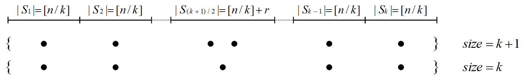
Figure 3: $t$-Closeness first, case $k$ does not divide $n$. Types of clusters when $k$ is odd. Top row, the data set is split into $k$ subsets. Central row, cluster with $k+1$ records. Bottom row, cluster with $k$ records.

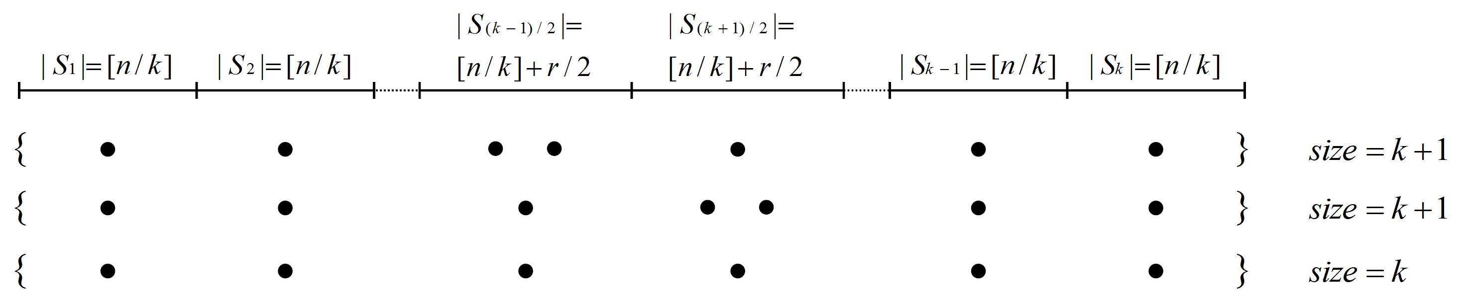
Figure 4: $t$-Closeness first, case $k$ does not divide $n$. Types of clusters when $k$ is even. Top row, the data set is split into $k$ subsets. Central rows, clusters with $k+1$ records (one with two records from $S_{(k-1)/2}$ and the other with two records from $S_{(k+1)/2}$). Bottom row, cluster with $k$ records.

Just as we did in Proposition 2, we can compute an upper bound for the EMD of the clusters depicted in Figures 3 and 4. The EMD of a cluster $C$ measures the cost of transforming the distribution of $C$ to the distribution of the data set. The cost of the probability mass redistribution can be computed in two steps as follows. First, we want the weight of each subset $S_{1},\ldots,S_{k}$ in cluster $C$ (the proportion of records in $C$ coming from each subset) to be equal to the weight of the subset in the data set; to this end, we redistribute the probability mass of the cluster between subsets. This redistribution cost, $cost_{0}$, equals the EMD between the cluster and the data set when the distributions have been discretized to the subsets. Then, for each subset $S_{i}\in\{S_{1},\ldots,S_{k}\}$, we compute $cost_{i}$, an upper bound of the cost of distributing the probability mass $|S_{i}|/n$ assigned to the subset among its elements (this is analogous to the mass distribution in the proof of Proposition 2). The EMD is the sum $cost_{0}+cost_{1}+\ldots+cost_{k}$. The fact that there are subsets with different sizes and there are clusters with different sizes makes formulas quite tedious and unwieldy, even though the resulting bounds on EMD are very similar to the one obtained in Proposition 2. For these reasons, we will use the latter as an approximation even when $k$ does not divide $n$; in particular, we will determine the cluster size using Expression (3).

Algorithm 3 formalizes the above described procedure to generate a $k$-anonymous $t$-close data set. It makes use of Expressions (3) and (4) to determine and adjust the cluster size, respectively.

Algorithm 3 $t$-Closeness-first microaggregation algorithm. Distances between records are computed in terms of the quasi-identifiers.

Data: $X$: original data set

          $n$: size of $X$

          $k$: minimum cluster size

          $t$: $t$-closeness level

Result Set of clusters satisfying $k$-anonymity and $t$-closeness

$k=\max\{k,\lceil\frac{n}{2(n-1)t+1}\rceil\}$

$k=k+\lceil(n\bmod k)/\lfloor n/k\rfloor\rceil$

$Clusters=\emptyset$

Split $X$ into $S_{1},\ldots,S_{k}$ subsets with $\lfloor n/k\rfloor$ records in ascending order of the confidential attribute, with any remaining $(n\bmod k)$ records assigned to the central subset(s)

while $X\neq\emptyset$ do

     $x_{a}$ = average record of $X$

     $x_{0}$ = most distant record from $x_{a}$ in $X$

     $C=\emptyset$

     for $i=1,\ldots,k$ do

         $x$ = closest record to $x_{0}$ in $S_{i}$

         $C=C\cup\{x\}$

         $S_{i}=S_{i}\setminus\{x\}$

         $X=X\setminus\{x\}$

         $\triangleright$ Take second record from $S_{i}$ if it contains extra records and no extra record has been already added to $C$

         if $|S_{i}|>|S_{1}|$ and $|C|=i$ then

              $x$ = closest record to $x_{0}$ in $S_{i}$

              $C=C\cup\{x\}$

              $S_{i}=S_{i}\setminus\{x\}$

              $X=X\setminus\{x\}$

         end if

     end for

     $Clusters=Clusters\cup\{C\}$

     if $X\neq\emptyset$ then

         $x_{1}$ = most distant record from $x_{0}$ in $X$

         $C=\emptyset$

         for $i=1,\ldots,k$ do

              $x$ = closest record to $x_{1}$ in $S_{i}$

              $C=C\cup\{x\}$

              $S_{i}=S_{i}\setminus\{x\}$

              $X=X\setminus\{x\}$

              if $|S_{i}|>|S_{1}|$ and $|C|=i$ then

                  $x$ = closest record to $x_{1}$ in $S_{i}$

                  $C=C\cup\{x\}$

                  $S_{i}=S_{i}\setminus\{x\}$

                  $X=X\setminus\{x\}$

              end if

         end for

         $Clusters=Clusters\cup\{C\}$

     end if

end while

return $Clusters$

In terms of computational cost, Algorithm 3 has a great advantage over Algorithms 1 and 2: when running Algorithm 3, we know that by construction the generated clusters satisfy $t$-closeness, so there is no need to compute any EMD distance. Algorithm 3 has cost $\mathcal{O}(n^{2}/k)$, the same cost order as MDAV (on which it is based). Actually, Algorithm 3 is even slightly more efficient than MDAV: all operations being equal, some of the computations that MDAV performs on the entire data set are performed by Algorithm 3 just on one of the subsets of $n/k$ records.

8 Empirical evaluation

In this section we empirically evaluate and compare the proposed algorithms using several data sets and according to different metrics: actual cluster size, speed and scalability, and data utility preservation.

8.1 Actual cluster size

In a first battery of tests we used as evaluation data the Census data set [1], which is usual to test privacy protection methods [32, 12, 6] and contains 1,080 records with numerical attributes. Similar to [6], we took attributes TAXINC (Taxable income amount) and POTHVAL (Total other persons income) as quasi-identifiers, and FEDTAX (Federal income tax liability) and FICA (Social Security retirement payroll deduction) as confidential attributes.

Because $k$-anonymity and $t$-closeness pursue different goals (the former clusters records with similar quasi-identifiers while the latter requires clusters with a distribution of confidential attributes similar to the one of the entire data set), we defined two data sets according to the correlation between the values of quasi-identifier and confidential attributes:

• Moderately correlated data set (MCD). It consists of 1,080 records with TAXINC and POTHVAL as quasi-identifier attributes, and FEDTAX as confidential attribute. The correlation between both types of attributes is 0.52. This represents the most usual scenario in which quasi-identifiers and confidential attributes show some correlation.

• Highly correlated data set (HCD). It uses the same quasi-identifiers as MCD, but it takes FICA as confidential attribute. The correlation between both types of attributes is 0.92. This highly correlated data set represents a worst-case scenario for our algorithms because, to fulfill a certain $t$-closeness level (i.e., to ensure a certain distribution of confidential values), we are likely to be forced to microaggregate records with significantly diverse quasi-identifier values, thereby incurring more information loss than in the MCD data set.

By applying the three algorithms to these two data sets for different values of $k$ and $t$, we will show how close to $k$ are the sizes of clusters formed by each algorithm for each value of $t$ to be enforced. To minimize information loss, the closer all cluster sizes to $k$, the better. The $k$ values have been taken in the range 2-30, which covers the most usual $k$-anonymity values (e.g. $k$ is taken between 3 and 10 in [4]), whereas the $t$ values have been taken in the range 0.01-0.25 (where 0.25 is the upper bound of $t$-closeness for this data set for the lowest $k$, that is $k=2$, according to Proposition 2).

We start by analyzing the behavior of Algorithm 1, in which records are first microaggregated in clusters of size $k$ that are thereafter merged until $t$-closeness is fulfilled. Table I shows the actual level of microaggregation that results from the merging process: minimum, that is, the size of the smallest cluster (which determines the actual $k$-anonymity level achieved), and average, that is, the average size of the merged clusters.

TABLE I: Algorithm 1: actual microaggregation (minimum and average size of the clusters, respectively) resulting for several values of $k$ and $t$ for the MCD and HCD data sets

	$t=0.01$		$t=0.05$		$t=0.09$		$t=0.13$		$t=0.17$		$t=0.21$		$t=0.25$
	MCD	HCD	MCD	HCD	MCD	HCD	MCD	HCD	MCD	HCD	MCD	HCD	MCD	HCD
$k=2$	1080/1080	1080/1080	56/120	36/98	20/42	16/31	8/20	8/52	4/10	4/9	4/7	4/7	2/8	2/5
$k=5$	1080/1080	1080/1080	385/540	200/216	40/154	40/60	20/47	20/80	10/24	10/21	10/17	10/15	5/12	5/11
$k=10$	1080/1080	1080/1080	1080/1080	1080/1080	110/270	180/216	40/108	40/190	20/57	20/47	20/35	20/31	10/24	10/20
$k=15$	1080/1080	1080/1080	1080/1080	495/540	135/360	195/270	45/90	60/270	30/64	30/68	30/45	30/54	15/33	15/33
$k=20$	1080/1080	1080/1080	380/540	240/360	160/216	180/216	80/154	60/140	40/83	40/72	40/54	40/60	20/37	20/40
$k=25$	1080/1080	1080/1080	1080/1080	1080/1080	1080/1080	230/360	455/540	50/250	50/180	50/98	50/90	50/72	25/72	25/48
$k=30$	1080/1080	1080/1080	540/540	1080/1080	270/360	330/540	120/180	150/390	60/98	60/108	60/77	60/90	30/57	30/57

It can be seen that, in many cases, the actual level of microaggregation is significantly higher than the value of $k$. This is undesirable because the larger the clusters, the higher the information loss. We also see that the size of the clusters tends to increase for both data sets as:

• i) the parameter $t$ of $t$-closeness decreases: since clusters have been created without considering the desired $t$-closeness, it is unlikely that they satisfy it as $t$ gets smaller. Thus, to decrease, if necessary, the distance between the distribution of confidential attributes within each cluster and over the entire data set, the algorithm merges the already created clusters (thereby increasing their cardinality); in the worst case (i.e., $t$ around 0.01-0.05), this implies grouping all 1,080 records in a single cluster.

• ii) the initial level of $k$-anonymity increases: the coarser the initial microaggregation, the more effort (i.e., merging) is needed to achieve a certain $t$-closeness level.

We also observe a noticeable difference between the minimum and average cardinality of the clusters, which suggests that the microggregation of records that we obtain in practice is far from optimal.

TABLE II: Algorithm 2: actual microaggregation (minimum and average size of the clusters, respectively) resulting for several values of $k$ and $t$ for the MCD and HCD data sets.

	$t=0.01$		$t=0.05$		$t=0.09$		$t=0.13$		$t=0.17$		$t=0.21$		$t=0.25$
	MCD	HCD	MCD	HCD	MCD	HCD	MCD	HCD	MCD	HCD	MCD	HCD	MCD	HCD
$k=2$	164/216	156/360	8/10	8/11	4/7	4/7	4/6	4/4	2/3	2/3	2/3	2/3	2/3	2/3
$k=5$	40/64	80/154	10/16	10/10	5/7	5/8	5/7	5/8	5/7	5/7	5/7	5/8	5/6	5/7
$k=10$	40/108	80/135	10/17	10/17	10/17	10/17	10/15	10/16	10/15	10/14	10/13	10/14	10/12	10/12
$k=15$	30/57	30/60	15/28	15/30	15/25	15/26	15/23	15/23	15/23	15/22	15/19	15/21	15/16	15/17
$k=20$	40/54	40/49	20/37	20/43	20/35	20/36	20/32	20/32	20/31	20/29	20/26	20/28	20/22	20/23
$k=25$	50/51	50/51	25/51	25/51	25/43	25/43	25/39	25/39	25/40	25/37	25/32	25/35	25/28	25/26
$k=30$	30/57	60/64	30/68	30/64	30/54	30/54	30/49	30/47	30/47	30/43	30/37	30/42	30/34	30/34

Table II shows the results for Algorithm 2. With this algorithm, we observe that the actual microaggregation levels are significantly smaller than in the previous case for the same values of $k$ and $t$, and so is the difference between the minimum and average cardinality of the clusters. Now $t$-closeness is enforced after creating each cluster rather than after creating all clusters. Thus, once a cluster is created, some of the $k$ records in that cluster may be replaced by unclustered records until $t$-closeness is satisfied; doing so does not increase the cardinality of the cluster, even though it may end up clustering records with less homogeneous quasi-identifiers and thereby yielding a higher loss of information. Only if the replacement does not satisfy the desired $t$-closeness, the clusters are merged like in Algorithm 1, thereby increasing the microaggregation level (in fact, as suggested in Section 6, we use Algorithm 2 as the microaggregation function of Algorithm 1). The results shown in Table II suggest that this process occurs for the smallest $t$-closeness values (i.e., 0.01-0.05), which are the ones that impose the strictest constraint.

The differences between the two data sets are more noticeable if we look at the average cardinality of the clusters: the HCD data set results in a larger average cardinality, because the initial clusters present more homogeneous confidential values (these are very correlated to the more homogeneous quasi-identifier values obtained for the first clusters) and tend to require more effort (i.e., replacements and mergers) to attain $t$-closeness.

TABLE III: Algorithm 3: actual microaggregation (minimum and average size of the clusters, respectively) resulting for several values of $k$ and $t$ for the MCD and HCD data sets.

	$t=0.01$		$t=0.05$		$t=0.09$		$t=0.13$		$t=0.17$		$t=0.21$		$t=0.25$
	MCD	HCD	MCD	HCD	MCD	HCD	MCD	HCD	MCD	HCD	MCD	HCD	MCD	HCD
$k=2$	49/49	49/49	10/10	10/10	6/6	6/6	4/4	4/4	3/3	3/3	3/3	3/3	2/2	2/2
$k=5$	49/49	49/49	10/10	10/10	6/6	6/6	5/5	5/5	5/5	5/5	5/5	5/5	5/5	5/5
$k=10$	49/49	49/49	10/10	10/10	10/10	10/10	10/10	10/10	10/10	10/10	10/10	10/10	10/10	10/10
$k=15$	49/49	49/49	15/15	15/15	15/15	15/15	15/15	15/15	15/15	15/15	15/15	15/15	15/15	15/15
$k=20$	49/49	49/49	20/20	20/20	20/20	20/20	20/20	20/20	20/20	20/20	20/20	20/20	20/20	20/20
$k=25$	49/49	49/49	25/25	25/25	25/25	25/25	25/25	25/25	25/25	25/25	25/25	25/25	25/25	25/25
$k=30$	49/49	49/49	30/30	30/30	30/30	30/30	30/30	30/30	30/30	30/30	30/30	30/30	30/30	30/30

Finally, Table III shows the results for Algorithm 3. Figures in this table show that Algorithm 3 is the one achieving an actual microaggregation level closest to the desired $k$. Moreover, since the cardinality of the data sets (1,080 records) is a multiple of the values of $k$, all clusters can be formed with the same cardinality $k$ (i.e., clusters are perfectly balanced). Indeed, as stated in Section 7, Algorithm 3 seeks the smallest clusters whose cardinality is at least $k$ and which satisfy a pre-specified level of $t$-closeness. To do so, it prioritizes the fulfillment of $t$-closeness over the homogeneity of quasi-identifiers in cluster formation. Because of this strategy, there are no differences between the MCD and HCD data sets; in fact, we can see that for most parameter choices and for both data sets the minimum and average cluster sizes are $k$.

In comparison with Algorithm 2, we observe that, even though in some cases (e.g., for $t=0.05$ and $k=2$) the minimum cardinality is greater with Algorithm 3, the average cardinality is always smaller with this algorithm. This is a consequence of the more precise microaggregation implemented by Algorithm 3.

8.2 Speed and scalability

The second part of the evaluation focuses on measuring the speed and scalability of the three algorithms with a larger data set.

To that end, we took a higher-dimensional data set from the the Patient Discharge Data for year 2010 of Californian hospitals, which are provided by California’s Office of Statewide Health Planning and Development [20]. We took the data set with the largest number of entries (Cedars Sinai Medical Center, with 55,668 patient records). From these, we removed records with missing attribute values and obtained a final data set with 23,435 records. Each record consists of 7 quasi-identifier attributes (e.g., patient’s age, zip code, admission date, etc.) plus one confidential attribute that specifies the amount charged for the patient’s stay in the hospital. The correlation between the quasi-identifier attributes and the confidential one is just 0.129.

The run time of the three algorithms for the Patient Discharge data set is shown in Figure 5 as a function of the value of $t$ to be attained. We set $k=2$ in order to give maximum freedom to the algorithms in adapting the microaggregation to the desired value of $t$ (again between 0.01 and the maximum upper bound of 0.25), and force them to create the greatest number of clusters (which the is worst case from the run time perspective).

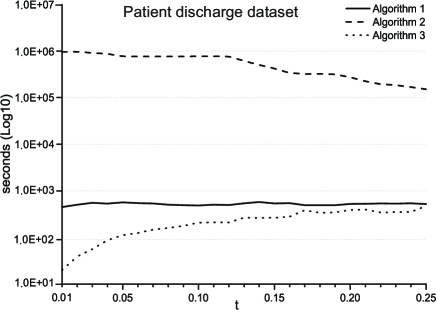
Figure 5: Run time (in seconds with $log_{10}$ scale) for the three algorithms with $k=2$ and values of $t$ between 0.02 and 0.25 for the Patient Discharge data set

Run time figures are coherent with the theoretical analysis of computational costs for the three algorithms. Algorithms  1 and  3 are significantly more efficient than Algorithm 2 (note the logarithmic scale of the Y-axis), because the former have just the quadratic cost of the underlying microaggregation algorithm, whereas the latter has a cubic cost resulting from the rearrangement of records required to fulfill $t$-closeness after the creation of each cluster. Indeed, Algorithm 2 may not scale well for large data sets, whereas the other two algorithms scale as well as the underlying microaggregation. At a closer look, Algorithm 3 is significantly more efficient than Algorithm 1 for low values of $t$. The reason is that, although the cost of both algorithms is $\mathcal{O}(n^{2}/k)$, Algorithm 3 optimally updates the value of $k$ in terms of the actual $t$: for small values of $t$, the value of $k$ is large (see Equation 3), which reduces the computational cost. In contrast, Algorithm 1 only takes $t$ into account after the entire microaggregation has been performed. Finally, the run time of Algorithm 2 tends to decrease for large $t$ because, in this case, clusters are more likely to (nearly) fulfill $t$-closeness, thus requiring less rearrangement of records after each iteration.

8.3 Data utility preservation

So far, the comparison between algorithms has been made only in terms of cluster sizes and run time. Let us now examine to what extent each algorithm preserves the data utility for a certain privacy level. Indeed, the different microaggregation strategies and the actual levels of microaggregation achieved by the three algorithms have a direct influence on the utility of the anonymized results. In the literature, the utility of an anonymized output is evaluated in terms of information loss, that is, the discrepancies between the original and the anonymized data set. The Sum of Squared Errors (SSE) is a well-known information loss measure, which is well-suited to capture the impact of creating equivalence classes by means of $k$-anonymous microaggregation. SSE is defined as the sum of squares of attribute distances between records in the original data set $X$ and their versions in the anonymized data set. However, since SSE provides absolute error values, we normalized it to obtain a measure that is independent of the data set size (number of records and attributes) and the ranges of attribute values:

$$SSE=\frac{1}{n}\sum_{x_{j}\in X}\frac{1}{m}\sum_{a_{j}^{i}\in x_{j}}(NED(a_{j}^{i},(a_{j}^{i})^{\prime}))^{2}$$ (5)

where $n$ is the number of records, $m$ is the number of attributes, $a_{j}^{i}$ is the value of the $i$-th attribute for the $j$-th original record, $(a_{j}^{i})^{\prime}$ represents its anonymized version and $NED(\cdot,\cdot)$ corresponds to the Normalized Euclidean Distance. Notice that with a high SSE, that is, a high information loss, a lot of data uses are severely damaged, like for example subdomain analyses (analyses restricted to parts of the data set).

To fairly and clearly compare the three algorithms, we first took $k=2$ for $k$-anonymity with $t$ values between 0.01 and 0.25 for $t$-closeness. In this manner, any actual cluster size $k>1$ is feasible and the algorithms have the greatest freedom to microaggregate records to fulfill the desired $t$-closeness. SSE values for each value of $t$ are shown in Figure 6 for the three data sets.

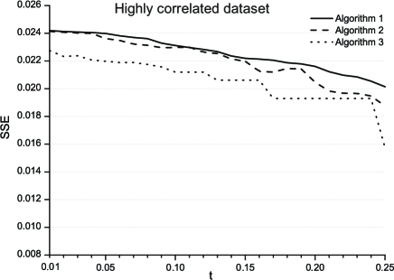
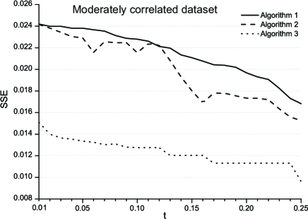
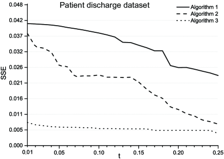
Figure 6: Normalized SSE values for the three algorithms with $k=2$ and values of $t$ between 0.02 and 0.25 for the HCD (top), MCD (middle) and Patient Discharge (bottom) data sets

All graphs show that Algorithm 2 improves on Algorithm 1 and, in turn, Algorithm 3 improves on Algorithm 2. Thus, we can see that the earlier we consider the fulfillment of $t$-closeness in the microaggregation step, the more utility is preserved in the output. This may seem paradoxical, because a $t$-closeness aware microaggregation that prioritizes the distribution of confidential values (such as the one in Algorithm 3) is likely to cluster records with heterogeneous quasi-identifier values, and thereby incur higher information loss. Some of this is apparent in Figure 6: Algorithm 3 improves much more on the other two algorithms for the MCD and Patient Discharge than for the HCD data set, because cluster homogeneity for HCD is harder to reconcile with the $t$-closeness requirement due to the higher correlation of quasi-identifiers and the confidential attribute. However, on the other hand, the fact that the $k$-anonymous microaggregation is aware of the level of $t$-closeness that should be satisfied also produces smaller clusters (of size closer to the desired $k$), which is beneficial to keep SSE low. In contrast, the other algorithms, and especially Algorithm 1, prioritize quasi-identifier values in the $k$-anonymous microaggregation and, hence, they require a lot of cluster merging and/or manipulation to attain $t$-closeness. This tends to produce larger clusters (as shown by the experiments on cluster sizes), whose aggregation incurs a greater loss of information, which is nonetheless fairly independent of the correlation between quasi-identifiers and confidential attributes; this is especially noticeable for the Patient Discharge data set, in which Algorithm 1 behaves significantly worse than the other two.

To sum up, the increase of information loss that the lower cluster homogeneity of $t$-closeness aware microaggregation might cause is more than compensated by the information loss reduction resulting from smaller clusters.

Finally, we also evaluated the evolution of the normalized SSE as a function of both $k$ and $t$. As a reference, Figure 7 shows this evolution for the three algorithms with the MCD data set.

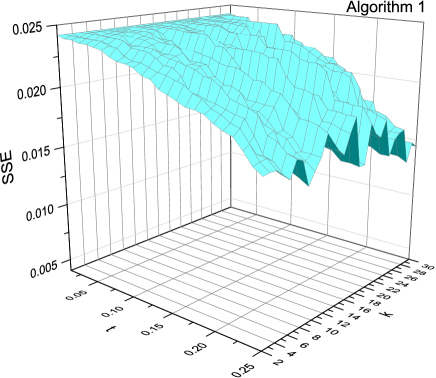
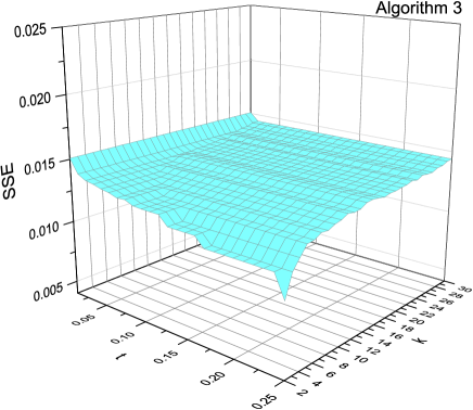
Figure 7: Normalized SSE for the three algorithms for $k$ between 2 and 30 and $t$ between 0.02 and 0.25 for the MCD data set

First, we can see that some of the advantages of Algorithm 3 are diminished when a higher $k$ is required. As shown in Proposition 2, the actual cluster size will be the maximum between the desired $k$ and the minimum size required to fulfill $t$-closeness. Thus, because of the optimal updating of $k$ by Algorithm 3, this algorithm is the one for which SSE increases the most as a result of the larger $k$. Algorithms 1 and 2, on the other hand, are more immune to large values of $k$. Indeed, since they prioritize the $k$-anonymous microaggregation, the larger clusters obtained for large values of $k$ have a greater chance to already fulfill $t$-closeness without the posterior merging step; since $k$-anonymous clusters are created in order to minimize the SSE, the smaller number of merging steps required to fulfill $t$-closeness helps to maintain cluster homogeneity and avoid increasing SSE. In any case, for any value of $k$, the SSE for these algorithms is still higher than for Algorithm 3.

For Algorithms 1 and 2, it is also interesting to observe the spikes that occur for certain values of $k$, which are more noticeable for Algorithm 1. Spikes occur when $k$ is not a divisor of the data set size $n$ (i.e., 1,080); that is, when it is not possible to group all records in clusters of size $k$. In such cases, the microaggregation algorithm is forced to distribute the remaining $r=n\bmod k$ records among already created clusters, which deteriorates cluster homogeneity and thus increases SSE. On the contrary, Algorithm 3 is more immune to this situation, because clusters are created to satisfy $t$-closeness, rather than to minimize the SSE.

9 Conclusions and research directions

We have proposed and evaluated the use of microaggregation as a method to attain $k$-anonymous $t$-closeness.

The a priori benefits of microaggregation vs generalization/recoding and local suppression have been discussed. Global recoding may recode more than needed, whereas local recoding complicates data analysis by mixing together values corresponding to different levels of generalization. Also, recoding produces a greater loss of granularity of the data, is more affected by outliers, and changes numerical values to ranges. Regarding local suppression, it complicates data analysis with missing values and is not obvious to combine with recoding in order to decrease the amount of generalization. Microaggregation is free from all the above downsides.

We have proposed and evaluated three different microaggregation based algorithms to generate $k$-anonymous $t$-close data sets. The first one is a simple merging step that can be run after any microaggregation algorithm. The other two algorithms, $k$-anonymity-first and $t$-closeness-first, take the $t$-closeness requirement into account at the moment of cluster formation during microaggregation. The $t$-closeness-first algorithm considers $t$-closeness earliest and provides the best results: smallest average cluster size, smallest SSE for a given level of $t$-closeness, and shortest run time (because the actual microaggregation level is computed beforehand according to the values of $k$ and $t$). Thus, considering the $t$-closeness requirement from the very beginning turns out to be the best option.

Since connections have been demonstrated between $t$-closeness and $\varepsilon$-differential privacy of data sets [27, 8], exploring how microaggregation could be leveraged to implement the latter model in the case of data releases is a natural continuation of this work. Moreover, we will also study the adaptation of the algorithms to support categorical data by: i) defining an EMD suitable to compare categorical values of different nature (e.g., ordinal values such as colors, which can be sorted within a range, or nominal values such as jobs, hobbies, diagnoses, etc., which require interpreting their underlying semantics), ii) defining aggregation operators to compute cluster centroids (i.e., the categorical value that minimizes the distance to other values in the same cluster), and iii) properly managing records with numerical and categorical attributes in an integrated manner.

Jordi Soria-Comas is a postdoctoral researcher at Universitat Rovira i Virgili. He has received his M. Sc. in Computer Security (2011) and Ph. D. in Computer Science (2013) degrees from the Universitat Rovira i Virgili. He also holds a M. Sc. in Finance from the Autonomous University of Barcelona (2004) and a B.Sc. in Mathematics from the University of Barcelona (2003). His research interests are in data privacy and security.

Josep Domingo-Ferrer (Fellow, IEEE) is a Distinguished Professor of Computer Science and an ICREA-Acadèmia Researcher at Universitat Rovira i Virgili, Tarragona, Catalonia, where he holds the UNESCO Chair in Data Privacy. He received the MSc and PhD degrees in Computer Science from the Autonomous University of Barcelona in 1988 and 1991, respectively. He also holds an MSc degree in Mathematics. His research interests are in data privacy, data security and cryptographic protocols. More information on him can be found at http://crises-deim.urv.cat/jdomingo

David Sánchez is an Associate Professor of Computer Science at Universitat Rovira i Virgili, Tarragona, Catalonia. His research interests are in data semantics and data privacy. He received a PhD in Computer Science from the Technical University of Catalonia. Contact him at david.sanchez@urv.cat.

Sergio Martínez is a post-doctoral researcher at University Rovira i Virgili (URV) in Tarragona. He received an MSc in Intelligent Systems (2010) and a Ph.D in Computer Science (2013), both awarded by the URV. His research interests are in artificial intelligence, semantic similarity and privacy preservation. He has participated in European and Spanish research projects.

References

- [1] R. Brand, J. Domingo-Ferrer, and J.M. Mateo-Sanz. Reference data sets to test and compare SDC methods for protection of numerical microdata. European Project IST-2000-25069 CASC. http://neon.vb.cbs.nl/casc/CASCtestsets.htm
- [2] J. Cao, P. Karras, P. Kalnis, and K.-L. Tan. SABRE: a Sensitive Attribute Bucketization and REdistribution framework for t-closeness. The VLDB Journal, 20(1):59-81, 2011.
- [3] D. Defays and P. Nanopoulos. Panels of enterprises and confidentiality: the small aggregates method. In Proceedings of the 1992 Symposium on Design and Analysis of Longitudinal Surveys, pp. 195–204, Ottawa, 1992. Statistics Canada.
- [4] J. Domingo-Ferrer and V. Torra. A quantitative comparison of disclosure control methods for microdata. In Confidentiality, Disclosure and Data Access: Theory and Practical Applications for Statistical Agencies (eds. L. Zayatz, P. Doyle, J. Theeuwes and J. Lane), pp. 111–134, Amsterdam, 2001. North Holland.
- [5] J. Domingo-Ferrer and J. M. Mateo-Sanz. Practical data-oriented microaggregation for statistical disclosure control. IEEE Transactions on Knowledge and Data Engineering, 14(1):189-201, 2002.
- [6] J. Domingo-Ferrer and U. González-Nicolás. Hybrid microdata using microaggregation. Information Sciences, 180(15):2834–2844, 2010.
- [7] J. Domingo-Ferrer, D. Sánchez and G. Rufian-Torrell. Anonymization of nominal data based on semantic marginality. Information Sciences, 242:35–48, 2013.
- [8] J. Domingo-Ferrer and J. Soria-Comas. From -closeness to differential privacy and vice versa in data anonymization. Knowledge-Based Systems, 74:151–158, 2015.
- [9] J. Domingo-Ferrer and V. Torra. Ordinal, continuous and heterogeneous k-anonymity through microaggregation. Data Min. Knowl. Discov., 11(2):195–212, 2005.
- [10] C. Dwork. Differential privacy. In Proc. of the 33rd Intl. Colloquium on Automata, Languages and Programming (ICALP 2006), LNCS 4052, pp. 1–12. Springer, 2006.
- [11] A. Hundepool, J. Domingo-Ferrer, L. Franconi, S. Giessing, E. S. Nordholt, K. Spicer, and P.-P. de Wolf. Statistical Disclosure Control. Wiley, 2012.
- [12] M. Laszlo and S. Mukherjee. Minimum spanning tree partitioning algorithm for microaggregation. IEEE Transactions on Knowledge and Data Engineering, 17(7):902–911, 2005.
- [13] K. LeFevre, D. J. DeWitt, and R. Ramakrishnan. Incognito: efficient full-domain k-anonymity. In Proceedings of the 2005 ACM SIGMOD International Conference on Management of Data (SIGMOD 2005), pp. 49–60, New York, NY, USA, 2005. ACM.
- [14] K. LeFevre, D. J. DeWitt, and R. Ramakrishnan. Mondrian multidimensional k-anonymity. In Proceedings of the 22nd International Conference on Data Engineering (ICDE 2006), Washington, DC, USA, 2006. IEEE Computer Society.
- [15] J. Li, R.C.-W. Wong, A.W.-C. Fu, and J. Pei. Anonymization by local recoding in data with attribute hierarchical taxonomies. IEEE Transactions on Knowledge and Data Engineering, 20(9):1181–1194, 2008.
- [16] N. Li, T. Li, and S. Venkatasubramanian. t-closeness: privacy beyond k-anonymity and l-diversity. In Proceedings of the 23rd IEEE International Conference on Data Engineering (ICDE 2007), pp. 106–115. IEEE, 2007.
- [17] N. Li, T. Li, and S. Venkatasubramanian. Closeness: a new privacy measure for data publishing. IEEE Transactions on Knowledge and Data Engineering, 22(7):943–956, 2010.
- [18] A. Machanavajjhala, D. Kifer, J. Gehrke, and M. Venkitasubramaniam. l-diversity: privacy beyond k-anonymity. ACM Trans. Knowl. Discov. Data, 1(1), 2007.
- [19] A. Oganian and J. Domingo-Ferrer. On the complexity of optimal microaggregation for statistical disclosure control. Statistical Journal of the United Nations Economic Comission for Europe, 18:345–354, 2001.
- [20] Patient Discharge Data. Office of Statewide Health Planning & Development-OSHPD, 2010. http://www.oshpd.ca.gov/HID/Products/PatDischargeData/PublicDataSet/index.html
- [21] D. Rebollo-Monedero, J. Forne, and J. Domingo-Ferrer. From t-closeness-like privacy to postrandomization via information theory IEEE Transactions on Knowledge and Data Engineering, 22(11):1623–1636, 2010,
- [22] Y. Rubner, C. Tomasi, and L. J. Guibas. The earth mover’s distance as a metric for image retrieval. International Journal of Computer Vision, 40(2):99–121, 2000.
- [23] P. Samarati and L. Sweeney. Protecting privacy when disclosing information: k-anonymity and its enforcement through generalization and suppression. In Proceedings of the IEEE Symposium on Research in Security and Privacy, 1998.
- [24] A. Solanas, A. Martínez-Ballesté. V-MDAV: Variable group size multivariate microaggregation. In Proceeding of the International Conference on Computational Statistics (COMPSTAT 2006), pp. 917–-925, 2006.
- [25] A. Solanas, F. Sebé, and J. Domingo-Ferrer. Micro-aggregation-based heuristics for p-sensitive k-anonymity: one step beyond. In Proceedings of the 2008 International Workshop on Privacy and Anonymity in Information Society (PAIS 2008), pp. 61–69, New York, NY, USA, 2008. ACM.
- [26] J. Soria-Comas and J. Domingo-Ferrer. Probabilistic k-anonymity through microaggregation and data swapping. In Proceedings of the IEEE International Conference on Fuzzy Systems (FUZZ-IEEE 2012), pp. 1–8. IEEE, 2012.
- [27] J. Soria-Comas and J. Domingo-Ferrer. Differential privacy via t-closeness in data publishing. In Proceedings of the 11th Annual International Conference on Privacy, Security and Trust (PST 2013), pp. 27–35, 2013.
- [28] J. Soria-Comas, J. Domingo-Ferrer, D. Sánchez and S. Martínez. Enhancing data utility in differential privacy via microaggregation-based -anonymity. VLDB Journal 23(5):771–794, 2014.
- [29] L. Sweeney. k-anonymity: a model for protecting privacy. International Journal of Uncertainty, Fuzziness and Knowledge-Based Systems, 10(5):557–570, 2002.
- [30] T. M. Truta and B. Vinay. Privacy protection: p-sensitive k-anonymity property. In Proceedings of the 2nd International Workshop on Privacy Data Management (PDM 2006), page 94. IEEE Computer Society, 2006.
- [31] X. Xiao and Y. Tao. Anatomy: simple and effective privacy preservation. In Proceedings of the 32Nd International Conference on Very Large Data Bases (VLDB 2006), pp. 139–150. VLDB Endowment, 2006.
- [32] W.E. Winkler, W. E. Yancey and R.H. Creecy. Disclosure risk assessment in perturbative microdata protection. In Inference Control in Statistical Databases, LNCS 2316, pp. 135–152. Springer, 2002.