Particle spectra and efficiency in nonlinear relativistic shock acceleration: survey of scattering models

Abstract

We include a general form for the scattering mean free path, $\lambda_{\mathrm{mfp}}(p)$, in a nonlinear Monte Carlo model of relativistic shock formation and Fermi acceleration. Particle-in-cell (PIC) simulations, as well as analytic work, suggest that relativistic shocks tend to produce short-scale, self-generated magnetic turbulence that leads to a scattering mean free path with a stronger momentum dependence than the $\lambda_{\mathrm{mfp}}\propto p$ dependence for Bohm diffusion. In unmagnetized shocks, this turbulence is strong enough to dominate the background magnetic field so the shock can be treated as parallel regardless of the initial magnetic field orientation, making application to $\gamma$-ray bursts (GRBs), pulsar winds, Type Ibc supernovae, and extra-galactic radio sources more straightforward and realistic. In addition to changing the scale of the shock precursor, we show that, when nonlinear effects from efficient Fermi acceleration are taken into account, the momentum dependence of $\lambda_{\mathrm{mfp}}(p)$ has an important influence on the efficiency of cosmic-ray production as well as the accelerated particle spectral shape. These effects are absent in non-relativistic shocks and do not appear in relativistic shock models unless nonlinear effects are self-consistently described. We show, for limited examples, how the changes in Fermi acceleration translate to changes in the intensity and spectral shape of $\gamma$-ray emission from proton-proton interactions and pion-decay radiation.
Keywords: acceleration of particles — ISM: cosmic rays — gamma-ray bursts — magnetohydrodynamics (MHD) — shock waves — turbulence

1. Introduction

Fermi shock acceleration at relativistic shocks may be an important cosmic-ray (CR) production mechanism in a number of sites including $\gamma$-ray bursts (GRBs), pulsar winds, type Ibc supernovae, and extra-galactic radio sources (see Bykov et al., 2012, for a review). Central to Fermi acceleration, as well as all other aspects of relativistic shock physics, is the production of the magnetic turbulence responsible for collisionless wave-particle interactions. Because of this, a great deal of work has been devoted studying plasma instabilities that may be important near relativistic shocks (see Lemoine & Pelletier, 2010; Rabinak et al., 2011; Plotnikov et al., 2013; Sironi et al., 2013; Lemoine et al., 2014; Reville & Bell, 2014, and references therein).

Despite this intense effort, the issue of particle transport in relativistic plasmas is by no means settled. In principle, particle-in-cell (PIC) simulations can solve the full problem of shock formation, wave generation, and particle acceleration self-consistently; and a great deal of work has been done with these techniques (e.g., Kato & Takabe, 2008; Spitkovsky, 2008; Nishikawa et al., 2009; Sironi et al., 2013). These simulations typically show the Weibel instability producing magnetic turbulence on skin-depth scales in the subshock vicinity and this self-generated turbulence can then lead to superthermal particle acceleration (e.g., Keshet et al., 2009; Haugbølle, 2011; Sironi & Spitkovsky, 2011).

The short-scale Weibel instability is critical in the initial shock formation process seen in PIC simulations, but Lemoine et al. (2014), for example, have shown that other longer-scale instabilities may develop in the shock precursor that dominate Weibel and modify the precursor structure in important ways. There are also indications from GRB afterglow observations that rapid Fermi acceleration and Bohm diffusion may occur in ultra-relativistic shocks (Sagi & Nakar, 2012). While PIC simulations are the only way to obtain fully self-consistent solutions, the computational limitations of PIC simulations (see Vladimirov et al., 2008) may be such that important nonlinear (NL) effects of Fermi acceleration on long-wavelength instabilities and shock precursor structure are currently beyond the reach of this technique.

In this paper we investigate the kinematics of first-order Fermi shock acceleration in relativistic shocks using a parameterized, momentum-dependent, scattering mean free path, $\lambda_{\mathrm{mfp}}(p)$, where $p$ is the local frame particle momentum. In particular, we examine the difference between a Bohm momentum dependence, i.e., $\lambda_{\mathrm{mfp}}\propto p$, and $\lambda_{\mathrm{mfp}}\propto p^{\alpha(p)}$, where $\alpha=2$ is expected from scattering off small-scale turbulence such as that generated by the Weibel instability (e.g., Jokipii, 1972; Plotnikov et al., 2011, 2013). While our parameterization cannot address fundamental issues concerning wave generation and shock formation, as done by PIC simulations or some semi-analytic models (e.g., Marcowith et al., 2006; Pelletier et al., 2009; Rabinak et al., 2011; Casse et al., 2013; Reville & Bell, 2014; Schlickeiser, 2015), we can model large spatial and momentum dynamic ranges and show how efficient Fermi acceleration varies with the momentum dependence of $\lambda_{\mathrm{mfp}}(p)$ when the backreaction of CRs on the shock precursor is included self-consistently.

The Monte Carlo simulation we employ has been described in detail in Ellison et al. (2013); Warren et al. (2015), and references therein (see Ellison & Double, 2002, for an early non-PIC discussion of NL Fermi acceleration in relativistic shocks). With this technique, the complex plasma physics of shock formation, magnetic turbulence generation, and particle acceleration (e.g., Sironi et al., 2013) is contained in the assumptions made to describe pitch-angle scattering and in our parameter $\alpha(p)$. We emphasize that the Monte Carlo simulation models particle transport not diffusion; an important distinction in relativistic shocks. No diffusion approximation is required and we can accurately follow particles as they scatter in plasmas moving at relativistic speeds with large velocity gradients.

Our main result is that, apart from a large change in length scale and the subsequent drop in the maximum accelerated particle energy for finite systems, the momentum dependence of $\lambda_{\mathrm{mfp}}(p)$ influences the shock structure and CR production in a purely relativistic fashion. We describe effects that do not occur in non-relativistic shocks, or in relativistic shocks where the backreaction of CRs on the shock structure is ignored. We find, for a given maximum CR momentum, $p_{\mathrm{max}}$, set by a finite shock size, that a strong momentum dependence for $\lambda_{\mathrm{mfp}}$ in NL shocks can produce a significant increase in the Fermi acceleration efficiency compared to that predicted with Bohm diffusion. This effect depends on the detailed momentum dependence of $\alpha(p)$.

As expected, any variation in the particle acceleration efficiency translates to a variation in the photon emissivity. We show, for some test parameters, that nonlinear effects can produce a factor of three enhancement, and a noticeable change in spectral shape, in the $10-100$ GeV pion-decay emissivity between Bohm diffusion and $\alpha(p)\sim 2$.

2. Details of Model

In our steady-state Monte Carlo model, particles, regardless of their momentum or position relative to the subshock, are assumed to interact with a turbulent background magnetic field so their pitch-angle-scattering mean free path is

$$\lambda_{\mathrm{mfp}}(p) = \eta_{\mathrm{mfp}}\cdot r_{g}(p_{d})\cdot(p/p_{d})^{\alpha_{L}}\quad\mathrm{for}\quad p<p_{d}$$ (1)

$$= \eta_{\mathrm{mfp}}\cdot r_{g}(p_{d})\cdot(p/p_{d})^{\alpha_{H}}\quad\mathrm{for}\quad p\geq p_{d}\ .$$

Here $p$ is the particle momentum in the local frame, $\alpha_{L}\leq 1$, $\alpha_{H}\geq 1$, $p_{d}$ is a dividing momentum between the low- and high-momentum ranges, $r_{g}(p_{d})=p_{d}c/(eB_{0})$ is the gyroradius for a proton with local-frame momentum $p_{d}$ in the background field $B_{0}$, and $\eta_{\mathrm{mfp}}\geq 1$ is a parameter that determines the strength of scattering. The Bohm limit is described by $\eta_{\mathrm{mfp}}=\alpha_{L}=\alpha_{H}=1$, and the conditions $\alpha_{L}\leq 1$ and $\alpha_{H}\geq 1$ ensure that $\lambda_{\mathrm{mfp}}\geq\eta_{\mathrm{mfp}}r_{g}$ for all $p$. In the simple geometry of our plane-parallel, steady-state model, results scale simply with $\eta_{\mathrm{mfp}}$ and we set $\eta_{\mathrm{mfp}}=1$ in all that follows. Discussions of the influence of $\eta_{\mathrm{mfp}}$ in unmodified, oblique relativistic shocks can be found in Ostrowski (1991); Ellison & Double (2004); Double et al. (2004); Summerlin & Baring (2012) (see Sagi & Nakar, 2012, for a discussion of $\eta_{\mathrm{mfp}}$ in GRB afterglows).

In the prescription given by equation (1), the background field $B_{0}$ (arbitrarily taken here to be $10^{-4}$ G) is assumed to be parallel to the shock normal and only sets the scale of the shock through $r_{g}(p_{d})$. Recent PIC simulations (i.e., Sironi et al., 2013) have shown that unmagnetized, relativistic shocks, regardless of their initial magnetic field orientation, develop strong, self-generated magnetic turbulence which quickly dominates the background field. The unmagnetized condition should apply to external afterglow shocks in GRBs, early-phase shocks in Type Ibc supernovae, and perhaps other astrophysical sites such as radio jets and pulsar winds. In these cases, the background field can be treated as parallel as we do here.

While equation (1) is a gross simplification of the wave-particle interactions that occur in relativistic plasmas, it does allow the investigation of basic particle transport effects in relativistic flows. Furthermore, if relativistic shocks accelerate CRs efficiently to ultra-high energies, as is often assumed (e.g., Kulkarni et al., 1999; Keshet & Waxman, 2005; Globus et al., 2015), important kinematic effects from momentum and energy conservation will occur regardless of the details of the plasma physics. These kinematic effects can be investigated with Monte Carlo techniques.

The only modification in the Monte Carlo model described in Warren et al. (2015) is that here we use equation (1) instead of $\lambda_{\mathrm{mfp}}=r_{g}$. Pitch-angle scattering is modeled as follows: after a time $\delta t\ll\tau_{g}$ ($\tau_{g}$ is the gyro-period) a particle scatters isotropically and elastically in the local plasma frame through a small angle $\delta\theta\leq\delta\theta_{\mathrm{max}}$. The maximum scattering angle in any scattering event is given by (see Ellison et al., 1990)

$$\delta\theta_{\mathrm{max}}=\sqrt{6\delta t/t_{c}}\ ,$$ (2)

where $\delta t=\tau_{g}/N_{g}$, $t_{c}=\lambda_{\mathrm{mfp}}/v$ is the collision time, $v$ is the particle speed in the local frame, and $N_{g}$ is a free parameter. In all examples here, $N_{g}$ is chosen large enough to produce fine-scattering results that do not change substantially as $N_{g}$ is increased further (see Summerlin & Baring, 2012, for test-particle examples with values of $N_{g}$ producing large-angle scattering).

All particles are injected far upstream with a thermal distribution and scatter and convect into and across the subshock into the downstream region. Upon interacting with the downstream plasma, a particle gains energy sufficient to allow it to scatter back across the subshock and be further accelerated. The fraction of particles that are injected, i.e., do manage to re-cross the subshock is determined stochastically and constitutes our “thermal leakage injection” model once the further assumption is made that the subshock is transparent. This injection model requires no additional parameters or assumptions once the scattering mean free path is defined in equation (1).

For our steady-state simulations, the $p_{\mathrm{max}}$ a shock can produce is determined by an upstream free escape boundary (FEB) parameter, $L_{\mathrm{FEB}}$, where $L_{\mathrm{FEB}}$ is the distance from the subshock to the FEB. In our plane-parallel shock approximation, a FEB mimics the effect of high-energy particles “leaking” from a finite-size shock (see Drury, 2011, for a fuller discussion of particle escape). In a finite shock, high-energy particles far upstream from the subshock have a high probability of escaping since the level of self-generated turbulence must decrease with upstream distance from the subshock. Particle escape could as well occur downstream from the subshock, as assumed in relativistic shock calculations by Achterberg et al. (2001) and Warren et al. (2015), or from the sides, as might be important in jets. How escape occurs will depend on the detailed geometry of the shock but all these scenarios produce a corresponding $p_{\mathrm{max}}$ with no important differences from what we describe here. An upstream FEB has been used extensively in models of CR production in young SNRs (e.g., Ellison et al., 2007; Morlino et al., 2009) where there is typically a SNR age where a transition occurs between $p_{\mathrm{max}}$ being determined by the remnant age to being determined by the finite shock radius. We note that there is direct observational evidence for upstream escape at the quasi-parallel Earth bow shock (e.g., Trattner et al., 2013).

With $L_{\mathrm{FEB}}$ set, the shock structure is determined so momentum and energy are conserved (see Ellison et al., 2013, for details). The injection rate adjusts consistently and the nonlinear examples we show below conserve momentum and energy to within a few percent.

We note that for unmodified (UM) shocks, where the backreaction of CRs is ignored, the model injects particles into the Fermi mechanism with an efficiency that is inconsistent with a discontinuous shock structure. With our injection model, momentum and energy can only be conserved if the backreaction of CRs on the shock structure is taken into account.

We further note that our UM examples are not test-particle (TP) ones, although TP predictions can be easily inferred from our UM results, as described in Warren et al. (2015). In a TP shock, injection must be weak enough so Fermi accelerated CRs are few enough so their influence on the shock structure can be ignored. The CR spectral shapes predicted for TP shocks are only applicable if an insignificant amount of energy is put into CRs.

Even though shock smoothing must occur if Fermi acceleration is efficient, we include UM/TP examples for several reasons. First, there is a universally accepted prediction for the power law slope for Fermi acceleration in UM/TP relativistic shocks that must be reproduced for a method to be valid (e.g., Bednarz & Ostrowski, 1998; Achterberg et al., 2001). We obtain this result within statistical limits. Second, the most obvious manifestation of the momentum dependence of $\lambda_{\mathrm{mfp}}$ is a simple scaling which can be most directly demonstrated with UM results. Finally, most other work on relativistic Fermi acceleration, other than PIC simulations, has been done in the TP approximation. We contrast UM and NL results to emphasize where nonlinear effects become important.

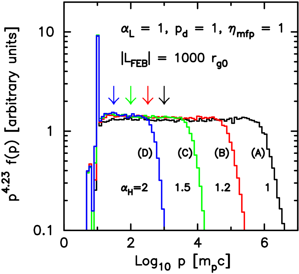
Figure 1.— Phase-space distributions measured at $x=0$ in the shock rest frame for various momentum dependencies for the mean free path parameters as indicated (see equation 1). The letters refer to the models listed in Table 1. In all cases, an upstream FEB at $x=-1000\,r_{g0}$ produced the high-momentum cutoff. Note that $p^{4.23}f(p)$ is plotted where $\sigma=4.23$ is the canonical test-particle power-law index for relativistic shock acceleration. The color-coded arrows indicate the momenta where $\lambda_{\mathrm{mfp}}(p)=|L_{\mathrm{FEB}}|$. These momenta are shown as dots in Fig. 2. In plane-parallel, non-relativistic shocks, such as models N and O discussed below, the arrows would be at $p_{\mathrm{max}}$ regardless of $\alpha_{H}$.

2.1. Particle Transport vs. Diffusion

Equations (1) and (2), along with the assumptions that particles scatter isotropically and elastically in the local plasma frame, in each scattering event, fully determine the particle transport in the Monte Carlo simulation. As shown in Ellison et al. (1990), equation (2) ensures that, on average, a particle in a uniform flow moves a displacement $\lambda_{\mathrm{mfp}}$ in acquiring a net deflection of $\sim 90^{\circ}$.

This particle transport model is more general than the diffusion-advection equation which is widely used in Fermi acceleration modeling. The Monte Carlo transport model accounts for an arbitrary particle anisotropy while the diffusion-advection equation accounts only for current anisotropy (i.e., the first Legendre polynomial in the particle pitch-angle distribution). If the scattering rate is high enough, and the background flows are extended and uniform, than to the first approximation both models would provide the same results. However, in weak scattering and/or in highly non-uniform, relativistic flows, the Monte Carlo transport treatment is more accurate. For example, a downstream particle crossing into the upstream region can, upon interacting with the upstream flow, suffer a small deflection and immediately be overtaken by the shock. Non-diffusive particle transport of this nature is essential for describing Fermi acceleration and is fully contained in equations (1) and (2).

3. Results

3.1. Unmodified Shocks

For UM shocks, the bulk flow is discontinuous with a transition from shock-frame speed $u_{0}$ for $x<0$ to $u_{2}$ for $x>0$. The shock compression ratio is defined as $R_{\mathrm{tot}}=u_{0}/u_{2}\simeq 3.02$ for the $\gamma_{0}=[1-(u_{0}/c)^{2}]^{-1/2}=10$ examples shown in Fig. 1 (see Double et al., 2004, for a detailed explanation of how $R_{\mathrm{tot}}$ is determined). In Fig. 1 we show particle phase-space distributions $f(p)$ ($\times p^{4.23}$) calculated in the shock rest frame at $x=0$ for different values of $\alpha_{H}$, all with $\alpha_{L}=1$, $p_{d}=m_{p}c$, $\eta_{\mathrm{mfp}}=1$, and an upstream FEB at $L_{\mathrm{FEB}}=-10^{3}\,r_{g0}$, where the scaling factor $r_{g0}\equiv\eta_{\mathrm{mfp}}m_{p}u_{0}c/(eB_{0})$. These examples assume an infinite downstream region and $L_{\mathrm{FEB}}$ solely determines $p_{\mathrm{max}}$. The letters in Fig. 1 indicate the models as listed in Table 1.

The mean free paths (equation 1) for Fig. 1 are shown in Fig. 2, where the horizontal dotted line is the position of the upstream FEB, i.e., $L_{\mathrm{FEB}}=-10^{3}\,r_{g0}\simeq-10^{-5}$ pc for the particular value $B_{0}=10^{-4}$ G chosen for these examples. The main effect in going from the Bohm limit ($\alpha_{H}=1$) to $\alpha_{H}=2$ is the decrease in $p_{\mathrm{max}}$ as the diffusion length at a given momentum increases with $\alpha_{H}$ and becomes comparable to $L_{\mathrm{FEB}}$. Except for some subtle effects at momenta just above $\gamma_{0}m_{p}c$, the superthermal spectral index has the canonical value $4.23$ and is independent of $\alpha_{H}$, as is the thermal leakage injection efficiency, in these UM examples. We discuss injection effects in more detail in Section 3.4.

3.2. Precursor Transport

Particle transport in the relativistic shock precursor differs considerably from that in non-relativistic shocks. For non-relativistic flows, the upstream diffusion length in an unmodified shock is

$$L_{\mathrm{diff}}=D/u_{0}=\lambda_{\mathrm{mfp}}v/(3u_{0})\ ,$$ (3)

where $D=\lambda_{\mathrm{mfp}}v/3$ is the diffusion coefficient. Setting $L_{\mathrm{diff}}=|L_{\mathrm{FEB}}|$, defining $L_{\mathrm{FEB}}^{\prime}=|L_{\mathrm{FEB}}|/r_{g0}$, $p_{d}^{\prime}=p_{d}/(m_{p}c)$, and taking $v\simeq c$, we have

$$L_{\mathrm{FEB}}^{\prime}=\frac{p_{d}^{\prime}}{3}\left(\frac{c}{u_{0}}\right)^{2}\left(\frac{p_{\mathrm{FEB}}}{p_{d}}\right)^{\alpha_{H}}\ ,$$ (4)

where

$$\lambda_{\mathrm{mfp}}=\eta_{\mathrm{mfp}}\cdot r_{g}(p_{d})\cdot(p/p_{d})^{\alpha_{H}}\ .$$ (5)

Therefore, the momentum associated with the diffusion distance to the upstream FEB is

$$p_{\mathrm{FEB}}=p_{d}^{\prime}\left[\frac{3L_{\mathrm{FEB}}^{\prime}}{p_{d}^{\prime}}\left(\frac{u_{0}}{c}\right)^{2}\right]^{1/\alpha_{H}}m_{p}c\ .$$ (6)

We include this well known result to emphasize that, while it is of fundamental importance for non-relativistic shocks and $p_{\mathrm{FEB}}\simeq p_{\mathrm{max}}$ regardless of $\alpha_{H}$ in the subset of non-relativistic shocks where Fermi acceleration is limited by an upstream FEB (see Section 3.7), it does not apply for relativistic flows.

In Fig. 1, $p_{d}^{\prime}=1$, $L_{\mathrm{FEB}}^{\prime}=1000$, $u_{0}\simeq c$, and we can estimate $p_{\mathrm{max}}$ for each $\alpha_{H}$ from the curves. We find: $(p_{\mathrm{FEB}}/p_{\mathrm{max}})_{\alpha_{H}=1}\simeq(3000/4\!\times\!10^{5})\simeq 7.5\!\times\!10^{-3}$, $(p_{\mathrm{FEB}}/p_{\mathrm{max}})_{\alpha_{H}=1.2}\simeq(790/5\!\times\!10^{4})\simeq 0.016$, $(p_{\mathrm{FEB}}/p_{\mathrm{max}})_{\alpha_{H}=1.5}\simeq(210/5\!\times\!10^{4})\simeq 0.05$, and $(p_{\mathrm{FEB}}/p_{\mathrm{max}})_{\alpha_{H}=2}\simeq(55/300)\simeq 0.2$. The fact that $p_{\mathrm{FEB}}/p_{\mathrm{max}}\ll 1$, and $p_{\mathrm{FEB}}/p_{\mathrm{max}}$ depends strongly on $\alpha_{H}$, shows the non-diffusive behavior of particle transport in the relativistic shock precursor as captured by the Monte Carlo simulation. In is noteworthy that, as the momentum dependence of $\lambda_{\mathrm{mfp}}$ increases, the particle transport approaches the non-relativistic diffusion length $D/u_{0}$. It is also noteworthy that the relation between $L_{\mathrm{FEB}}$ and $L_{\mathrm{diff}}$ will vary continuously as the shock Lorentz factor drops as it will during the GRB afterglow phase.

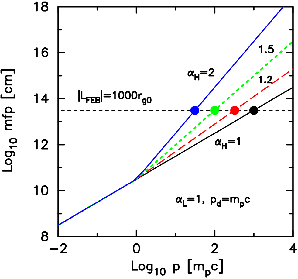
Figure 2.— Mean free path for the models A$-$D shown in Fig. 1 as indicated by $\alpha_{H}$. The upstream FEB is shown as a horizontal dotted line. The dots highlight the momentum needed in each case to produce a $\lambda_{\mathrm{mfp}}$ equal to $|L_{\mathrm{FEB}}|$.

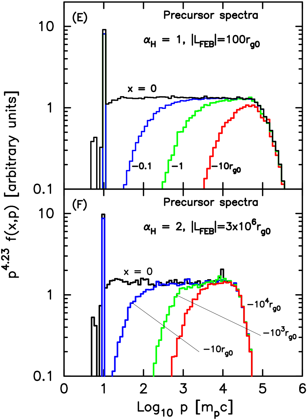
Figure 3.— The top panel shows shock-frame precursor spectra for an $\alpha_{H}=1$ example with $L_{\mathrm{FEB}}=-100\,r_{g0}$ (Model E). The position ahead of the subshock where $f(x,p)$ was calculated is indicated for each curve. The bottom panel shows shock-frame precursor spectra for Model F with $\alpha_{H}=2$, $p_{d}=m_{p}c$, and $L_{\mathrm{FEB}}=-3\!\times\!10^{6}\,r_{g0}$.

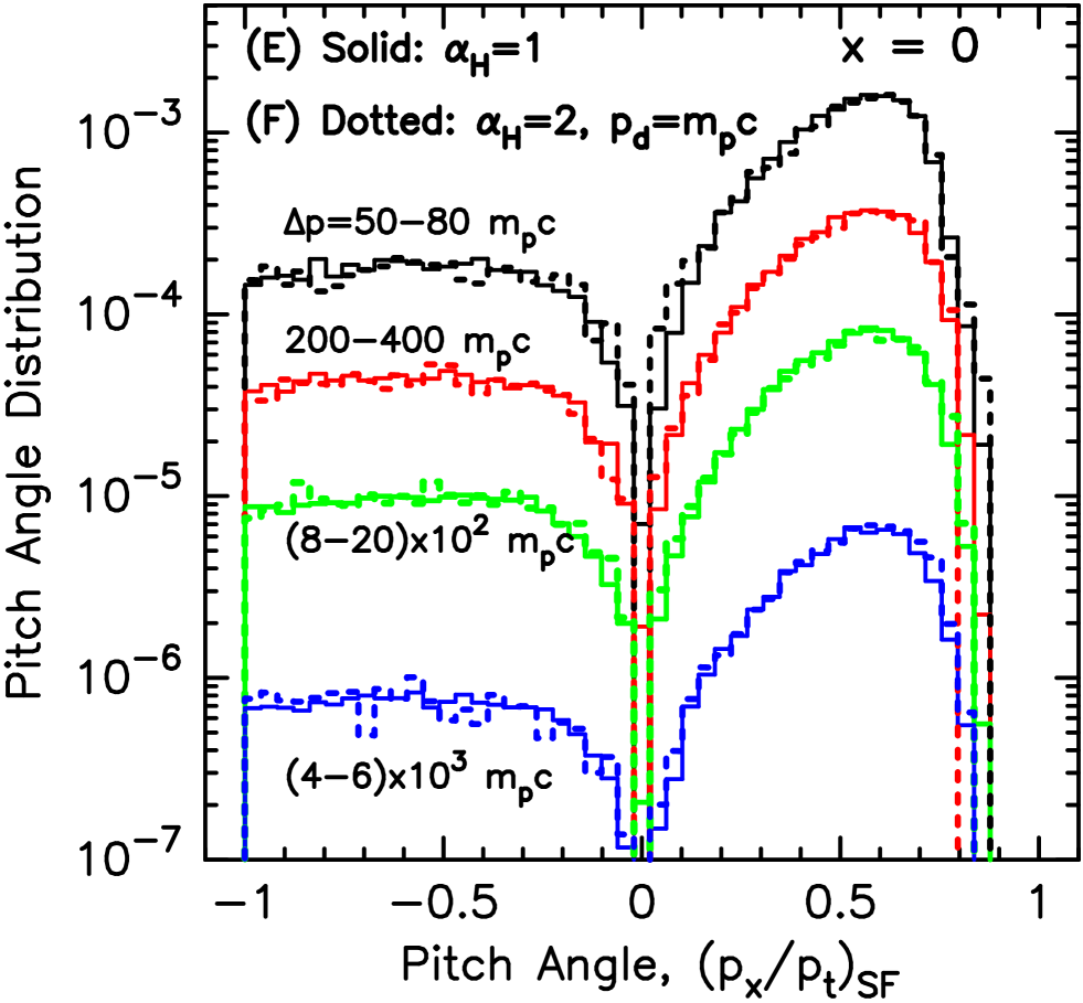
Figure 4.— Pitch-angle distributions for the $\alpha_{H}=1$ (solid curves, Model E) and $\alpha_{H}=2$, $p_{d}=m_{p}c$ (dotted curves, Model F) examples shown in Fig. 3 calculated at $x=0$. The distributions are calculated in the shock frame for four momentum ranges as indicated. All curves are normalized to the total injected particle flux so they are absolutely normalized relative to each other. The ratio $(p_{x}/p_{t})_{\mathrm{SF}}$ is the $x$-component of momentum divided by the total momentum measured in the shock-rest frame. A particle with $(p_{x}/p_{t})_{\mathrm{SF}}=1$ points directly downstream and, in the shock rest frame, no particle crosses $x=0$ with $(p_{x}/p_{t})_{\mathrm{SF}}=0$.

3.3. Precursor Spectra

In Fig. 3 we show $f(x,p)$ calculated at various positions, $x$, in the shock precursor as indicated. The top panel (Model E in Table 1) is for the Bohm limit, i.e., $\alpha_{H}=1$, while the bottom panel (Model F) has $\alpha_{H}=2$ with $p_{d}=m_{p}c$. The curve labeled $x=0$ in both panels displays the canonical $\sigma=4.23$ spectral index above the quasi-thermal peak and below the cutoff caused by the upstream FEB. The large difference in transport length between Bohm and $\alpha_{H}=2$ shows up in the relation between $L_{\mathrm{FEB}}$ and $p_{\mathrm{max}}$. In the Bohm limit, $L_{\mathrm{FEB}}^{\prime}=100$ yields $p_{\mathrm{max}}$ approximately 10 times as large as in the $\alpha_{H}=2$ example with $L_{\mathrm{FEB}}^{\prime}=3\!\times\!10^{6}$.

In both cases, the precursor spectra show that shocked particles scatter back upstream in an energy dependent fashion. It is noteworthy that this upstream transport readily occurs even though the speed difference between the accelerated particles and the bulk upstream flow is small, i.e., $u_{0}/c\simeq 0.995$ for $\gamma_{0}=10$. If particle scattering is assumed as in equation (1), the relativistic nature of the flow has no qualitative effect on the particle transport, other than the effect on $p_{\mathrm{FEB}}$ discussed in Section 3.1.

Particles crossing the subshock at $x=0$ are highly anisotropic in the shock frame, but the anisotropy is essentially independent of momentum, as shown in Fig. 4 for four particle momentum ranges. This momentum independence of the pitch-angle distribution, which is also independent of $\gamma_{0}$ for fully relativistic shocks, results in a power law with the canonical TP spectral index (e.g., Keshet & Waxman, 2005).

Fig. 4 also shows that, to within statistics, the subshock crossing anisotropy is independent of the momentum dependence of $\lambda_{\mathrm{mfp}}$ when the shock is unmodified. We note that these pitch-angle distributions are all normalized to the total injected number flux so they are absolutely normalized relative to each other.

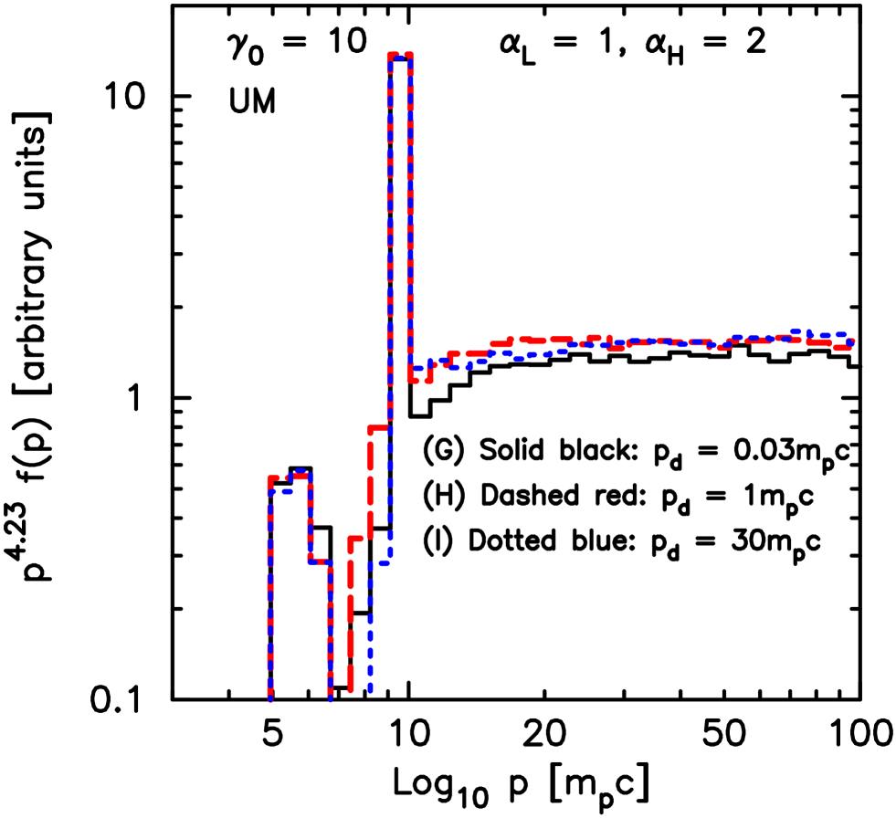
Figure 5.— Low-momentum phase-space distributions for $\alpha_{H}=2$ with various $p_{d}$ as indicated. In all cases the Fermi acceleration is limited by setting $p_{\mathrm{max}}\gg 100\,m_{p}c$ and the spectra are calculated in the shock frame at $x=0$. While the differences in the spectra are mostly from statistical noise, the variation between the $p_{d}=0.03\,m_{p}c$ spectrum and the other two just above the thermal peak may be real, albeit a consequence of the thermal leakage scheme assumed.

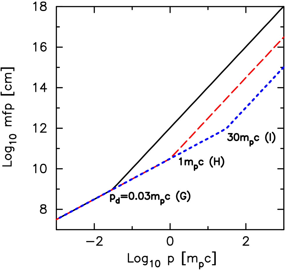
Figure 6.— Mean free path for Models G, H, and I as shown in Fig. 5.

3.4. Injection in UM Shocks

In order to investigate how the momentum dependence of $\lambda_{\mathrm{mfp}}$ influences particle injection, we show in Fig. 5 the low-momentum range of $f(p)$ for $\alpha_{H}=2$ for different values of $p_{d}$, as shown in Fig. 6. These examples all have $\alpha_{L}=\eta_{\mathrm{mfp}}=1$, and we limit particle acceleration by setting an upstream FEB that is large enough in each case so $p_{\mathrm{max}}\gg 100\,m_{p}c$ for all $p_{d}$. Concentrating on the low-energy part of $f(p)$, we see in Fig. 5 that $p_{d}$ has only a small effect on injection in these unmodified shocks. For the factor of 1000 range in $p_{d}$, the normalization of $f(p)$ at $15-100\,m_{p}c$ varies by less than 15%, most of which is statistical noise. We show below that $p_{d}$ has a much larger effect on Fermi acceleration in self-consistent, modified shocks.

It is interesting to note that there are peaks in Fig. 5 below $p=\gamma_{0}m_{p}c$ at $p\sim 6m_{p}c$. These are produced by downstream particles making their first crossing back into the upstream region. These particles have momenta less than $p=\gamma_{0}m_{p}c$ when measured in the shock frame. If the spectra in Fig. 5 were plotted in the far upstream rest frame, peaks at $\sim\gamma_{0}^{2}\,m_{p}c$ would be present.

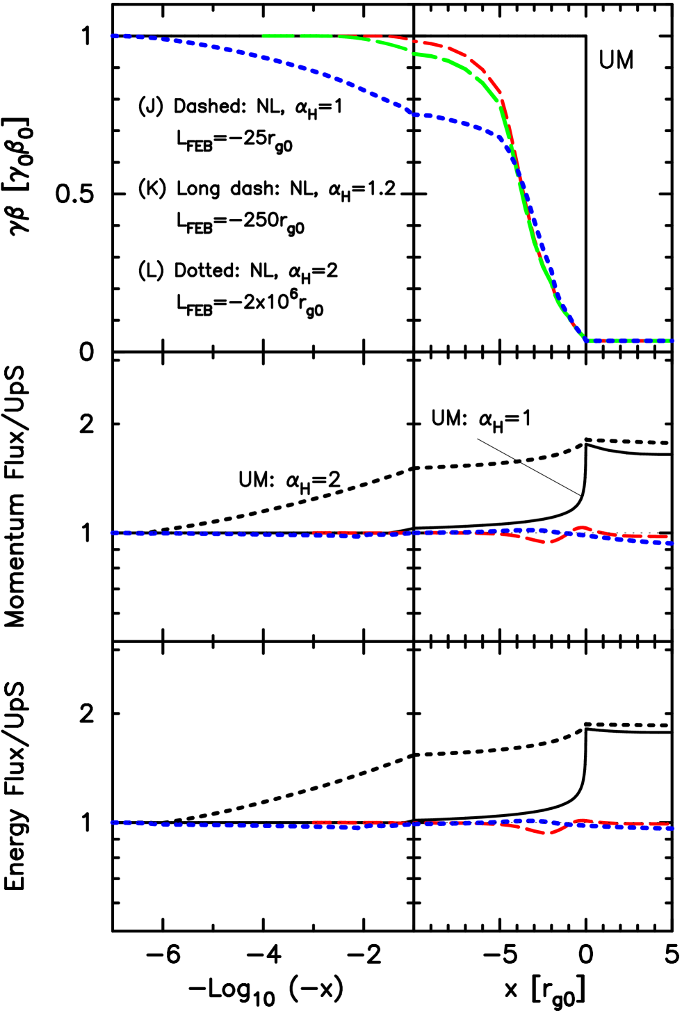
Figure 7.— The top panels show the NL shock structure in terms of the inverse density, $\gamma(x)\beta(x)/(\gamma_{0}\beta_{0})$, for shocks with different $\alpha_{H}$ and with upstream FEBs set to produce approximately the same $p_{\mathrm{max}}$, as shown in Fig. 9. The middle and bottom panels show the momentum and energy fluxes scaled to far upstream values. The dashed (red, Model J), long-dashed (green, Model K), and dotted (blue, Model L) curves show self-consistent NL results, while the black curves show UM results, as indicated. The momentum and energy fluxes for the $\alpha_{H}=1.2$ case are not shown in the middle and bottom panels for clarity.

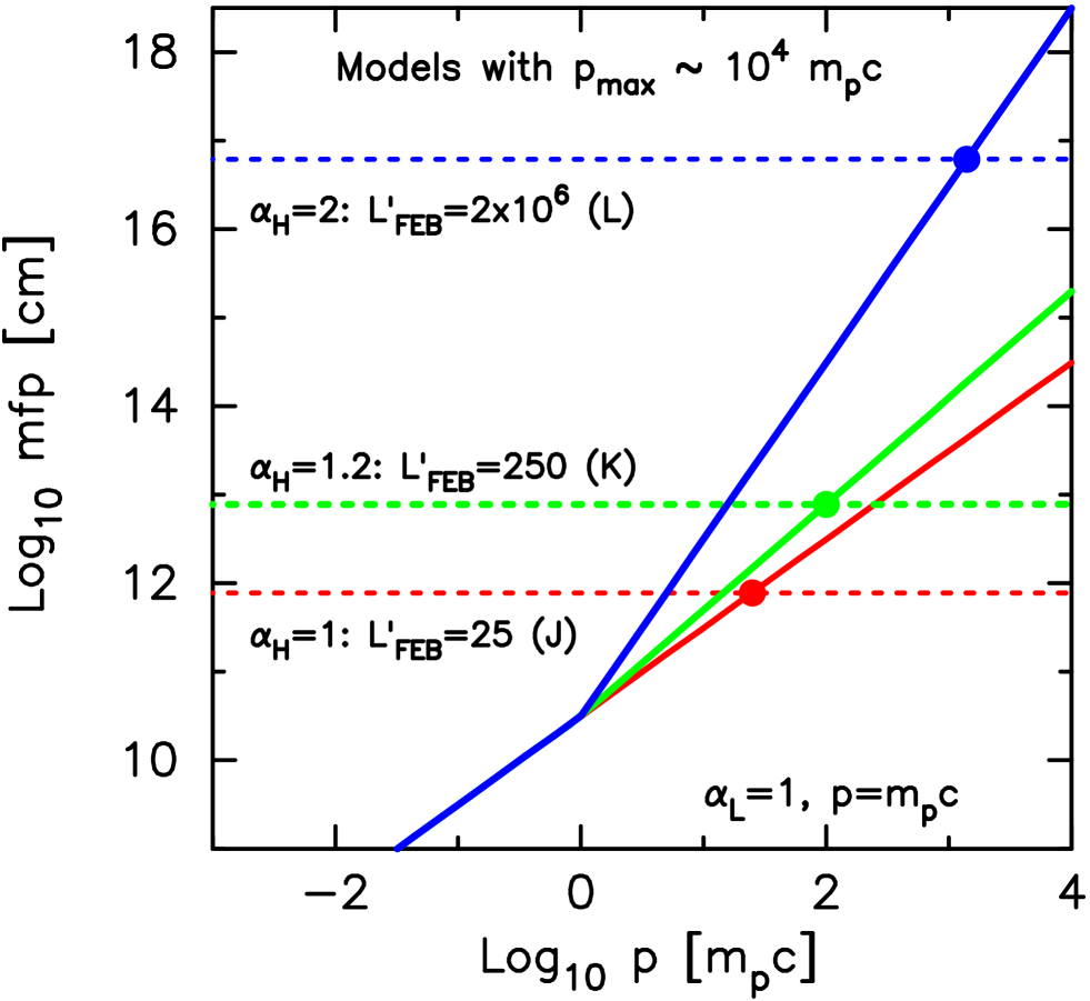
Figure 8.— Mean free paths for the self-consistent shocks shown in Figs. 7 and 9. The positions of the FEBs are shown and it is noted that the momenta at which $\lambda_{\mathrm{mfp}}(p_{\mathrm{FEB}})\simeq|L_{\mathrm{FEB}}|$ (solid dots) are such that $p_{\mathrm{FEB}}/p_{\mathrm{max}}$ is a strong increasing function of $\alpha_{H}$.

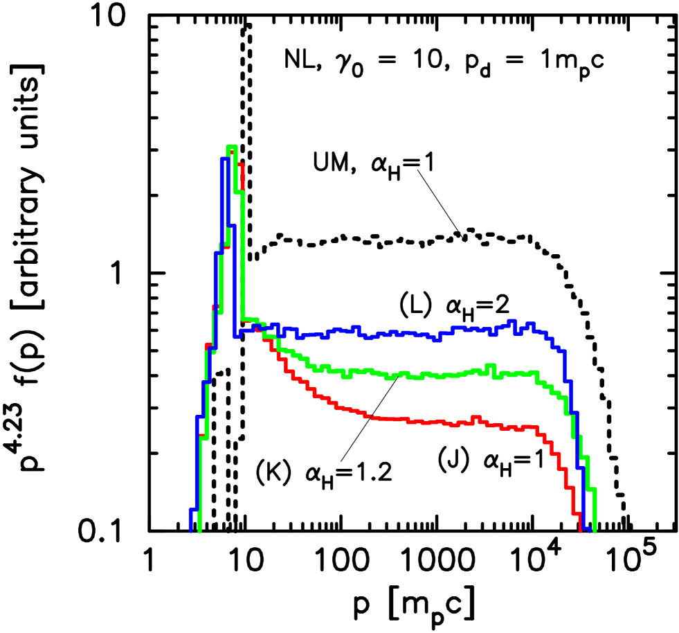
Figure 9.— The lower three spectra are from the self-consistent shocks shown in Fig. 7 with different $\alpha_{H}$ as indicated. For comparison we show the spectrum for an UM shock with $\alpha_{H}=1$ (dotted black curve). All spectra are calculated in the shock frame at $x=0$ and multiplied by $p^{4.23}$.

3.5. Nonlinear Shocks

We have shown that, other than a change in length scale and $p_{\mathrm{max}}$, the momentum dependence of $\lambda_{\mathrm{mfp}}$ has no important influence on Fermi acceleration in UM shocks, at least within the assumptions and approximations of our Monte Carlo model. We now investigate nonlinear shocks and show that the momentum dependence of $\lambda_{\mathrm{mfp}}$ produces important differences beyond a simple scaling.

In Fig. 7 we show self-consistent results for three values of $\alpha_{H}$ with $\alpha_{L}=p_{d}=1$ (models J, K, and L). In these examples, the upstream FEB has been set to produce approximately the same $p_{\mathrm{max}}\simeq 10^{4}\,m_{p}c$ for the three NL shocks (Fig 9). The top panels show inverse density profiles, $n_{0}/n(x)=\gamma(x)\beta(x)/(\gamma_{0}\beta_{0})$, where $\gamma(x)$ and $\beta(x)$ are measured in the shock rest frame. Here and elsewhere the subscript “0” indicates far upstream values. The mean free paths for these examples are shown in Fig. 8.

The self-consistent shock profiles shown as dashed ($\alpha_{H}=1$, red), long-dashed ($\alpha_{H}=1.2$, green), and dotted ($\alpha_{H}=2$, blue) curves in the top panels of Fig. 7 conserve momentum and energy fluxes to within a few percent, as indicated in the middle and bottom panels. This is in contrast to the UM shocks (solid and dotted black curves) where the momentum and energy fluxes in the downstream region are well above the far upstream values. Note the long extension of the momentum and energy fluxes into the precursor for the UM $\alpha_{H}=2$ case (black dotted curves), and the much shorter extension for the UM $\alpha_{H}=1$ case.

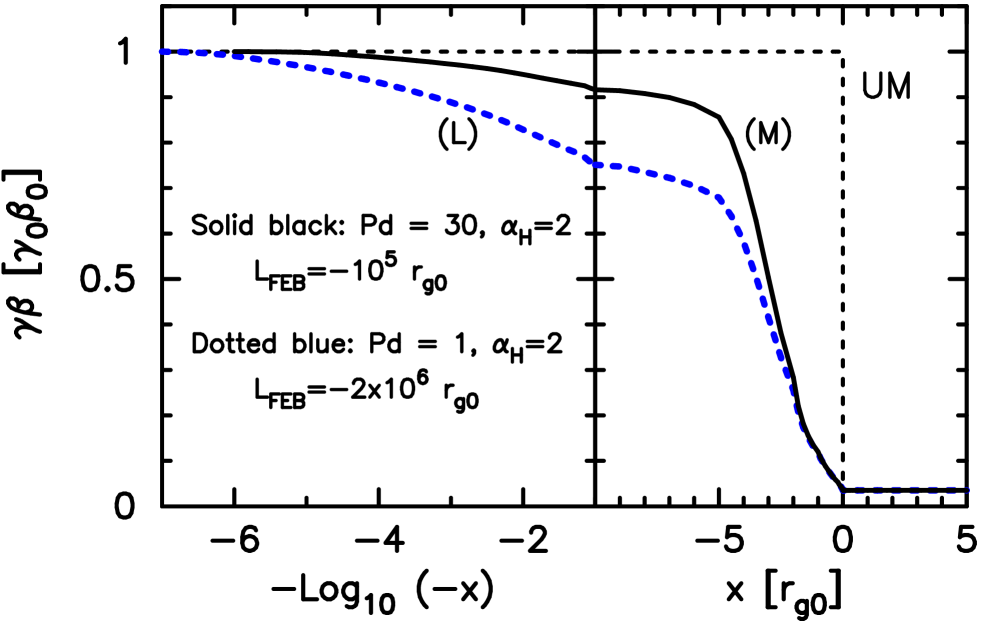
Figure 10.— The NL shock structure in terms of the inverse density, $\gamma(x)\beta(x)/(\gamma_{0}\beta_{0})$, for shocks with $\alpha_{H}=2$ and different $p_{d}$ as indicated. In both cases, the upstream FEB has been chosen to produce a $p_{\mathrm{max}}$ similar to the NL examples in Fig. 9. While not shown, as in Fig. 7, the momentum and energy fluxes are conserved to within a few percent for the NL cases.

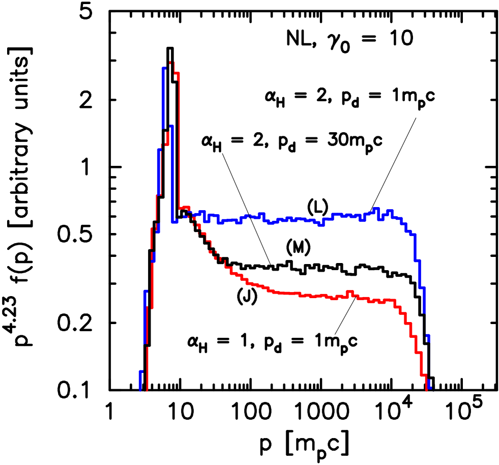
Figure 11.— Phase-space distributions with various $\alpha_{H}$ and $p_{d}$, as indicated. The J and L models are identical to those shown in Fig. 9. Note the effect $p_{d}$ has on the Fermi acceleration efficiency in the top two curves both with $\alpha_{H}=2$. All spectra are calculated in the shock frame at $x=0$.

In Fig. 9, we show the shock-frame spectra calculated at $x=0$ for each model in Fig. 7. The momentum dependence of $\lambda_{\mathrm{mfp}}$ has a striking effect on $f(p)$. The Bohm limit case ($\alpha_{H}=1$, Model J) shows the concave upward curvature characteristic of nonlinear Fermi acceleration in non-relativistic shocks (e.g., Ellison & Eichler, 1984) but this curvature is almost absent for $\alpha_{H}=2$ with $p_{d}=1$ (Model L). The NL spectra in Fig. 9 are absolutely normalized so they contain, within statistical limits, the same total particle and energy fluxes. The lack of curvature for large $\alpha_{H}$ results in a significant increase in the acceleration efficiency and there is a slight shift of the thermal peak toward lower momentum to accommodate this change in efficiency. At $\sim 1000\,m_{p}c$ the NL $\alpha_{H}=2$ spectrum is $>$2 times as intense as the $\alpha_{H}=1$ spectrum.

The modification of the Fermi acceleration efficiency seen in Fig. 9 depends importantly on $p_{d}$ as well as $\alpha_{H}$. In Figs. 10 and 11 we compare results for $p_{d}=1$ (Model L) and $30\,m_{p}c$ (Model M) when $\alpha_{H}=2$. For the $p_{d}=30\,m_{p}c$ example (black solid curves in Figs. 10 and 11) we have adjusted the upstream FEB to give approximately the same $p_{\mathrm{max}}$ as the NL examples shown in Fig. 9. The spectrum with $p_{d}=30\,m_{p}c$ is now closer to the $p_{d}=m_{p}c$ case.

When upstream thermal particles cross the shock the first time and interact with the downstream plasma, they obtain a plasma frame momentum of $\simeq 10\,m_{p}c$. For a $\lambda_{\mathrm{mfp}}$ break at $p_{d}=1\,m_{p}c$ between $\alpha_{H}=1$ and $\alpha_{H}=2$, these upstream thermal particles obtain mean free paths roughly $500\,r_{g0}$ long. This allows them to scatter far upstream from the subshock and treat much of the smooth shock transition as essentially unmodified. With $p_{d}=1\,m_{p}c$ this effect should increase smoothly as $\alpha_{H}$ goes from 1 to 2 since the scattering length is increasing but the shock structure isn’t changing significantly (as seen in Fig. 7). If the break point occurs above the downstream thermal peak at, for example $p_{d}=30\,m_{p}c$, the mean free path for particles below this momentum will be much less. In Fig. 11, the $\alpha_{H}=1$ ($p_{d}=m_{p}c$) and $\alpha_{H}=2$ ($p_{d}=30\,m_{p}c$) spectra behave similarly up to the separation momentum at $p=30\,m_{p}c$. Particles with $p<p_{d}$ feel the smooth shock structure and obtain the concave shape. For $p>p_{d}$, the $\alpha_{H}=1$ and $\alpha_{H}=2$ distributions separate. As Fig. 11 clearly shows, the form of $\alpha(p)$ will influence NL Fermi acceleration significantly.

In Table 1, we define the particle acceleration efficiency, ${\cal E}_{\mathrm{DSA}}$, for our NL $\gamma_{0}=10$ models as the fraction of energy flux above 1 TeV, measured in the shock frame. Since we are not attempting to fit a particular object with realistically derived parameters, ${\cal E}_{\mathrm{DSA}}$ is intended only as a measure of the relative shock acceleration efficiency for the various models. Table 1 shows that Model L with $\alpha_{H}=2$ puts approximately twice the energy into $>$TeV protons as does Model J with $\alpha_{H}=1$.

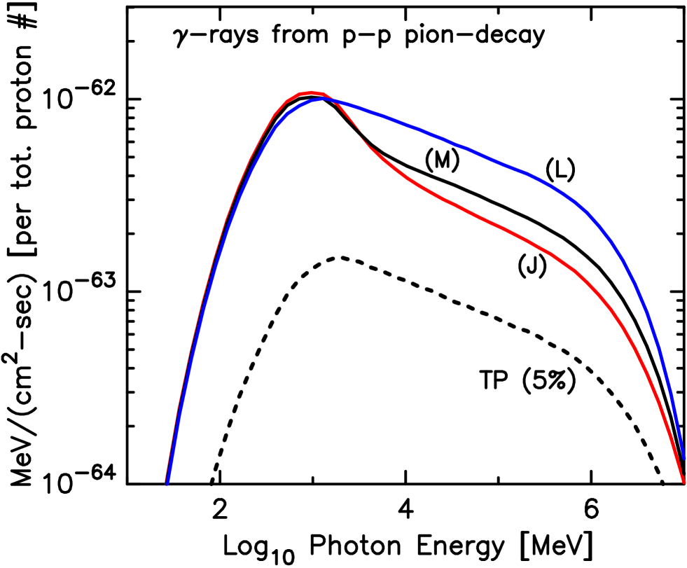
Figure 12.— Local plasma frame $\gamma$-ray emission due to $\pi^{0}$-decay produced in inealstic collisions of accelerated protons for the models shown in Fig. 11. Model J has $\alpha_{H}=1$, model L has $\alpha_{H}=2$ with $p_{d}=m_{p}c$, and model M has $\alpha_{H}=2$ with $p_{d}=30\,m_{p}c$. These spectra have an arbitrary absolute scale but are normalized to total proton number in each emitting region to isolate the effects from a varying $p$-dependence for $\lambda_{\mathrm{mfp}}$. The pion-decay emission is calculated using parameterizations given by Kamae et al. (2006, 2007) and Kelner et al. (2009). The dotted curve is the TP $\gamma$-ray emission for model J parameters assuming that 5% of the proton energy flux goes into Fermi accelerated CRs.

3.6. Pion-decay Emission

In Fig. 12 we show the $\pi^{0}$-decay $\gamma$-ray emission from the protons shown in Fig. 11. The density of the ambient material for the proton-proton interactions is determined self-consistently within the NL shock structure, i.e., from $\gamma(x)\beta(x)$ in Figs. 7 and 10. The spectra in Fig. 12 are normalized to the number of protons in the shock acceleration region and thus emphasize the NL effects from shock smoothing. As described in detail in Warren et al. (2015), the photon emission depends on the number of particles in the region between the upstream and downstream FEBs. For a given $p_{\mathrm{max}}$, the spatial extent of the shock, and the absolute normalization of the radiation, depend strongly on both $\alpha_{H}$ and $p_{d}$.

Fig. 12 shows that in addition to this simple scaling, NL effects from shock smoothing can produce a significant enhancement of the photon emission from that expected from the Bohm limit. Fig. 12 also shows that the spectral shape of the pion-decay emission in the 1-100 GeV range is modified substantially by NL effects. The dotted curve in the figure is the TP result where we have arbitrarily assumed that 5% of the proton energy flux is put into Fermi accelerated particles. At 100 GeV, the photon emission from the TP result is a factor of three or more below any of the NL models. Note that for a given $p_{\mathrm{max}}$, the TP result does not depend on $\alpha_{H}$ or $p_{d}$.

For simplicity, we have not included the acceleration of electrons or the leptonic emission here but similar effects can be expected (see Warren et al., 2015, for a discussion of electron acceleration and emission). We believe the NL effects from the momentum dependence of $\lambda_{\mathrm{mfp}}$ may be important for a detailed modeling of objects containing relativistic shocks, such as GRBs, but this is beyond the scope of this paper and is left for future work.

Figure 13.— Shock structure for non-relativistic shocks (i.e., $\gamma_{0}=1.002$) with two values of $\alpha_{H}$, as indicated. For the $\alpha_{H}=1.5$ example, $p_{d}=0.01\,m_{p}c$. The upstream FEB has been set to produce approximately the same $p_{\mathrm{max}}$, as shown in Fig. 14. As is well known for non-relativistic shocks undergoing efficient shock acceleration, the overall shock compression ratio must increase above the Rankine-Hugoniot value (e.g., Jones & Ellison, 1991; Berezhko & Ellison, 1999). For these examples, $R_{\mathrm{tot}}\simeq 12$.

Figure 14.— Shock frame distributions calculated at $x=0$ for the Model N and O shocks shown in Fig. 13. The self-consistent shock structure adjusts to produce approximately identical CR distributions despite the large change in precursor scale produced by the change in the $p$-dependence of $\lambda_{\mathrm{mfp}}$. These two examples are extremely efficient with ${\cal E}_{\mathrm{DSA}}\sim 0.8$, where ${\cal E}_{\mathrm{DSA}}$ is defined as the fraction of proton energy flux above $m_{p}c$ for non-relativistic shocks, as in Table 1.

3.7. Nonlinear, Nonrelativistic Shocks

To confirm that in parallel, non-relativistic shocks, our Monte Carlo code gives results that are independent of the momentum dependence of $\lambda_{\mathrm{mfp}}$, we show NL shock structures and spectra for two values of $\alpha_{H}$ in Figs. 13 and 14 for shocks with $\gamma_{0}=1.002$ ($u_{0}\simeq 1.9\!\times\!10^{4}$ km s^-1). The $\alpha_{H}=1.5$ example has $p_{d}=0.01\,m_{p}c$. As in Fig. 7, the upstream FEB has been adjusted to give approximately the same $p_{\mathrm{max}}$ for each case. Fig. 13 shows the large difference in precursor scale caused by $\alpha_{H}$ but Fig. 14 shows that the CR distribution functions are almost identical. In contrast to relativistic shocks, the momentum dependence of $\lambda_{\mathrm{mfp}}$ has no effect on nonlinear Fermi acceleration in non-relativistic shocks, other than the change in scale, as long as they are parallel and simple thermal leakage injection is assumed.

The two examples in these figures also confirm that, to within statistics, $p_{\mathrm{FEB}}=p_{\mathrm{max}}$, where $p_{\mathrm{FEB}}$ is defined in equation (6). For more details on NL Fermi acceleration  in non-relativistic shocks, the reader is directed to Berezhko & Ellison (1999); Malkov & Drury (2001); Caprioli et al. (2010); Bykov et al. (2014) and references therein.

4. Conclusions

Using a generalized form for the pitch-angle scattering mean free path, $\lambda_{\mathrm{mfp}}(p)\propto p^{\alpha(p)}$, in a kinematic Monte Carlo model making specific scattering assumptions, we have investigated how the momentum dependence of $\lambda_{\mathrm{mfp}}$ influences Fermi acceleration in relativistic shocks. Our main results are summarized below.

(1) For a given shock size the increase in scattering length produced by a strong momentum dependence for $\lambda_{\mathrm{mfp}}$ dramatically reduces the maximum energy a given shock can produce (Fig. 1).

(2) Superthermal particles can readily move into the shock precursor (Fig. 3) as for non-relativistic flows, but the particle transport no longer obeys the simple $D/u_{0}$ relation for the UM precursor diffusion length as in non-relativistic shocks (i.e., equation 4): particles must obtain a greater momentum to reach an upstream FEB than $D/u_{0}$ suggests (i.e., equation 6). Precursor transport approaches the non-relativistic expression as the strength of the momentum dependence of $\lambda_{\mathrm{mfp}}$ increases.

(3) In unmodified shocks (those that ignore the backreaction of accelerated particles), adjusting $\lambda_{\mathrm{mfp}}(p)$ has no important effects beyond the change in $p_{\mathrm{max}}$. Both the power-law spectral index (Fig. 1) and the thermal leakage injection efficiency (Fig. 5) are nearly independent of $\lambda_{\mathrm{mfp}}$ as long as test-particle conditions are assumed.

(4) Once the nonlinear interaction between the bulk flow and the accelerated particles is considered, both the injection efficiency and accelerated particle spectral shape depend significantly on the momentum dependence assumed for $\lambda_{\mathrm{mfp}}(p)$ (Figs. 7 and 9).

(5) If the upstream FEB is adjusted to produce a similar maximum CR energy, NL shocks with a momentum dependence for $\lambda_{\mathrm{mfp}}(p)$ stronger than Bohm (i.e., $\lambda_{\mathrm{mfp}}\propto p^{\alpha(p)}$ with $\alpha(p)>1$), inject and accelerate CRs more efficiently than in the Bohm limit. This effect comes about solely from the transport properties as determined by equation (1) and does not occur in NL, non-relativistic shocks or in relativistic shocks where the backreaction of CRs on the shock structure is ignored.

(6) The increase in Fermi acceleration efficiency produces a corresponding increase in the $\gamma$-ray emissivity for $\alpha(p)>1$ for self-consistent models (Fig. 12). For the parameters used here, NL effects can produce a factor of three enhancement in the pion-decay  flux between $\alpha(p)=1$ and $2$ in the $10-100$ GeV range. In this energy range, the pion-decay spectrum can be noticeably harder for large $\alpha(p)$ compared to the Bohm limit. An even larger difference in $\gamma$-ray emissivity is predicted between TP approximations and NL shocks with thermal leakage injection.

Particle-in-cell  simulations have shown that unmagnetized relativistic shocks can be efficient particle accelerators (e.g., Sironi et al., 2013) regardless of magnetic field geometry. The unmagnetized condition should apply for GRB external shocks producing afterglow emission, the early-time blast waves for particularly powerful supernovae, and possibly other sources containing relativistic shocks. If Fermi acceleration is efficient in these cases (and the $\sim 10\%$ efficiencies reported by Sironi et al., 2013, lower limits considering the limited box size and run times of the PIC simulations, are in line with what we obtain in our NL models) the NL effects of this acceleration must be considered for a self-consistent description of the shock formation and structure, magnetic turbulence generation, and CR production.

The self-generation of magnetic turbulence, and the particle scattering that results from it, are critical and poorly understood components of collisionless shock formation and Fermi acceleration. A great deal of work has been done studying the generation of magnetic turbulence in test-particle, relativistic shocks with semi-analytic and hydrodynamic techniques (e.g., Pelletier et al., 2009; Delaney et al., 2012; Guidorzi et al., 2014; Bosch-Ramon, 2015), but the nonlinear problem with efficient Fermi acceleration has not yet been adequately addressed with these techniques.

Indeed, at present the full self-consistent problem can only be solved with PIC simulations, and an important result of that work is the demonstration that the Weibel instability produces short-wavelength turbulence close to the subshock layer, i.e., within a few hundred ion skin depths (see Eq. 6 in Sironi et al., 2013). Particles moving through turbulence with scales much shorter than their gyroradius will scatter with $\lambda_{\mathrm{mfp}}\propto p^{2}$, very different from the generally assumed Bohm diffusion. Particle-in-cell simulations, however, are computationally intensive and are limited in box size, run time, and dimensionality (see Jones et al., 1998; Vladimirov et al., 2008). It is still an open question whether instabilities can be self-generated further into the shock precursor on scales comparable to the particle gyroradius (e.g., Sagi & Nakar, 2012; Lemoine et al., 2014).

If relativistic shocks in astrophysics do, in fact, efficiently Fermi accelerate CRs to ultra-high energies (e.g., Globus et al., 2015), they must somehow produce long-wavelength magnetic turbulence in the shock precursor and computationally fast techniques are required to model the resultant Fermi acceleration. The Monte Carlo model we have presented here concentrates on the NL kinematics and parameterizes the particle transport, assuming it can be produced well into the precursor. The transport model is more general than the diffusion-advection equation widely used in Fermi acceleration and can account for an arbitrary particle anisotropy.

Of course, many important aspects of relativistic shocks remain in question and we make no claim that our Monte Carlo simulation is a first-principles calculation. The models presented here, for instance, assume a plane shock and have no position dependence for $\lambda_{\mathrm{mfp}}(p)$. While PIC simulations show that magnetic turbulence is produced near the subshock and in the shock precursor, it may decay rapidly downstream from the subshock in a wavelength-dependent fashion. Using fundamental PIC results to guide simple parameterizations, future work will include a position and momentum-dependent mean free path, as well as the calculation of plasma instabilities self-consistently within the Monte Carlo code, as has been done for non-relativistic shocks (e.g., Vladimirov et al., 2006, 2009; Bykov et al., 2011, 2014). Anisotropic scattering can also be modeled using PIC results to guide the parameterization.

A further extension of this work is application to the evolving conditions of a GRB afterglow. Significant progress has already been made in this area, starting shortly after the first afterglow observations with the analytic work of Sari et al. (1998) and references therein. In recent years the traditional power-law electron distribution has been coupled to relativistically correct hydrodynamics calculations (e.g., Leventis et al., 2012; van Eerten & MacFadyen, 2013), allowing for rapid estimation of key GRB parameters from the afterglow light curves and spectra. However, a key feature of these models is their assumption that non-thermal electrons form a single power law with constant spectral index. We have shown here and in earlier work (Ellison et al., 2013; Warren et al., 2015) that the acceleration process is subject to many uncertainties, and that a simple power law may be insufficient to describe the particle distribution at any particular instant in time, let alone for a substantial fraction of the afterglow. A preliminary treatment of nonlinear DSA in the context of afterglows was presented in Warren (2015), and further study is planned.

Table 1Model Parameters.

Model	Type	$\gamma_{0}$	$\alpha_{H}$	$p_{d}$ [$m_{p}c$]	$|L_{\mathrm{UpS}}|$ [$r_{g0}$]	${\cal E}_{\mathrm{DSA}}$
A	UM	10	1	1	$10^{3}$	…
B	UM	10	1.2	1	$10^{3}$	…
C	UM	10	1.5	1	$10^{3}$	…
D	UM	10	2	1	$10^{3}$	…
E	UM	10	1	1	100	…
F	UM	10	2	1	$3\!\times\!10^{6}$	…
G	UM	10	2	0.03	…	…
H	UM	10	2	1	…	…
I	UM	10	2	30	…	…
J	NL	10	1	1	25	0.08
K	NL	10	1.2	1	250	0.12
L	NL	10	2	1	$2\!\times\!10^{6}$	0.15
M	NL	10	2	30	$10^{5}$	0.1
N	NL	1.002	1	1	$2.2\!\times\!10^{4}$	0.8
O	NL	1.002	1.5	0.01	$2.8\!\times\!10^{6}$	0.8

References

- Achterberg et al. (2001) Achterberg, A., Gallant, Y. A., Kirk, J. G., & Guthmann, A. W. 2001, MNRAS, 328, 393
- Bednarz & Ostrowski (1998) Bednarz, J. & Ostrowski, M. 1998, Physical Review Letters, 80, 3911
- Berezhko & Ellison (1999) Berezhko, E. G. & Ellison, D. C. 1999, ApJ, 526, 385
- Bosch-Ramon (2015) Bosch-Ramon, V. 2015, Astronomy and Astrophysics, 575, A109
- Bykov et al. (2012) Bykov, A., Gehrels, N., Krawczynski, H., et al. 2012, Space Sci. Rev., 173, 309
- Bykov et al. (2014) Bykov, A. M., Ellison, D. C., Osipov, S. M., & Vladimirov, A. E. 2014, ApJ, 789, 137
- Bykov et al. (2011) Bykov, A. M., Osipov, S. M., & Ellison, D. C. 2011, MNRAS, 410, 39
- Caprioli et al. (2010) Caprioli, D., Kang, H., Vladimirov, A. E., & Jones, T. W. 2010, MNRAS, 407, 1773
- Casse et al. (2013) Casse, F., Marcowith, A., & Keppens, R. 2013, MNRAS, 433, 940
- Delaney et al. (2012) Delaney, S., Dempsey, P., Duffy, P., & Downes, T. P. 2012, MNRAS, 420, 3360
- Double et al. (2004) Double, G. P., Baring, M. G., Jones, F. C., & Ellison, D. C. 2004, Astrophysical Journal, 600, 485
- Drury (2011) Drury, L. O. 2011, MNRAS, 415, 1807
- Ellison & Double (2002) Ellison, D. C. & Double, G. P. 2002, Astroparticle Physics, 18, 213
- Ellison & Double (2004) Ellison, D. C. & Double, G. P. 2004, Astroparticle Physics, 22, 323
- Ellison & Eichler (1984) Ellison, D. C. & Eichler, D. 1984, Astrophysical Journal, 286, 691
- Ellison et al. (1990) Ellison, D. C., Jones, F. C., & Reynolds, S. P. 1990, Astrophysical Journal, 360, 702
- Ellison et al. (2007) Ellison, D. C., Patnaude, D. J., Slane, P., Blasi, P., & Gabici, S. 2007, Astrophysical Journal, 661, 879
- Ellison et al. (2013) Ellison, D. C., Warren, D. C., & Bykov, A. M. 2013, ApJ, 776, 46
- Globus et al. (2015) Globus, N., Allard, D., Mochkovitch, R., & Parizot, E. 2015, MNRAS, 451, 751
- Guidorzi et al. (2014) Guidorzi, C., Mundell, C. G., Harrison, R., et al. 2014, MNRAS, 438, 752
- Haugbølle (2011) Haugbølle, T. 2011, The Astrophysical Journal Letters, 739, L42
- Jokipii (1972) Jokipii, J. R. 1972, Astrophysical Journal, 172, 319
- Jones & Ellison (1991) Jones, F. C. & Ellison, D. C. 1991, Space Science Reviews, 58, 259
- Jones et al. (1998) Jones, F. C., Jokipii, J. R., & Baring, M. G. 1998, Astrophysical Journal, 509, 238
- Kamae et al. (2006) Kamae, T., Karlsson, N., Mizuno, T., Abe, T., & Koi, T. 2006, Astrophysical Journal, 647, 692
- Kamae et al. (2007) Kamae, T., Karlsson, N., Mizuno, T., Abe, T., & Koi, T. 2007, Astrophysical Journal, 662, 779
- Kato & Takabe (2008) Kato, T. N. & Takabe, H. 2008, The Astrophysical Journal Letters, 681, L93
- Kelner et al. (2009) Kelner, S. R., Aharonian, F. A., & Bugayov, V. V. 2009, Phys. Rev. D, 79, 039901
- Keshet et al. (2009) Keshet, U., Katz, B., Spitkovsky, A., & Waxman, E. 2009, The Astrophysical Journal Letters, 693, L127
- Keshet & Waxman (2005) Keshet, U. & Waxman, E. 2005, Physical Review Letters, 94, 111102
- Kulkarni et al. (1999) Kulkarni, S. R., Djorgovski, S. G., Odewahn, S. C., et al. 1999, Nature, 398, 389
- Lemoine & Pelletier (2010) Lemoine, M. & Pelletier, G. 2010, MNRAS, 402, 321
- Lemoine et al. (2014) Lemoine, M., Pelletier, G., Gremillet, L., & Plotnikov, I. 2014, MNRAS, 440, 1365
- Leventis et al. (2012) Leventis, K., van Eerten, H. J., Meliani, Z., & Wijers, R. A. M. J. 2012, MNRAS, 427, 1329
- Malkov & Drury (2001) Malkov, M. A. & Drury, L. 2001, Reports of Progress in Physics, 64, 429
- Marcowith et al. (2006) Marcowith, A., Lemoine, M., & Pelletier, G. 2006, Astronomy and Astrophysics, 453, 193
- Morlino et al. (2009) Morlino, G., Amato, E., & Blasi, P. 2009, MNRAS, 392, 240
- Nishikawa et al. (2009) Nishikawa, K.-I., Niemiec, J., Hardee, P. E., et al. 2009, The Astrophysical Journal Letters, 698, L10
- Ostrowski (1991) Ostrowski, M. 1991, MNRAS, 249, 551
- Pelletier et al. (2009) Pelletier, G., Lemoine, M., & Marcowith, A. 2009, MNRAS, 393, 587
- Plotnikov et al. (2011) Plotnikov, I., Pelletier, G., & Lemoine, M. 2011, Astronomy and Astrophysics, 532, A68
- Plotnikov et al. (2013) Plotnikov, I., Pelletier, G., & Lemoine, M. 2013, MNRAS, 430, 1280
- Rabinak et al. (2011) Rabinak, I., Katz, B., & Waxman, E. 2011, Astrophysical Journal, 736, 157
- Reville & Bell (2014) Reville, B. & Bell, A. R. 2014, MNRAS, 439, 2050
- Sagi & Nakar (2012) Sagi, E. & Nakar, E. 2012, Astrophysical Journal, 749, 80
- Sari et al. (1998) Sari, R., Piran, T., & Narayan, R. 1998, The Astrophysical Journal Letters, 497, L17
- Schlickeiser (2015) Schlickeiser, R. 2015, Astrophysical Journal, 809, 124
- Sironi & Spitkovsky (2011) Sironi, L. & Spitkovsky, A. 2011, Astrophysical Journal, 726, 75
- Sironi et al. (2013) Sironi, L., Spitkovsky, A., & Arons, J. 2013, ApJ, 771, 54
- Spitkovsky (2008) Spitkovsky, A. 2008, The Astrophysical Journal Letters, 673, L39
- Summerlin & Baring (2012) Summerlin, E. J. & Baring, M. G. 2012, Astrophysical Journal, 745, 63
- Trattner et al. (2013) Trattner, K. J., Allegrini, F., Dayeh, M. A., et al. 2013, Journal of Geophysical Research (Space Physics), 118, 4425
- van Eerten & MacFadyen (2013) van Eerten, H. & MacFadyen, A. 2013, Astrophysical Journal, 767, 141
- Vladimirov et al. (2006) Vladimirov, A., Ellison, D. C., & Bykov, A. 2006, ApJ, 652, 1246
- Vladimirov et al. (2008) Vladimirov, A. E., Bykov, A. M., & Ellison, D. C. 2008, Astrophysical Journal, 688, 1084
- Vladimirov et al. (2009) Vladimirov, A. E., Bykov, A. M., & Ellison, D. C. 2009, The Astrophysical Journal Letters, 703, L29
- Warren (2015) Warren, D. C. 2015, PhD thesis, North Carolina State University
- Warren et al. (2015) Warren, D. C., Ellison, D. C., Bykov, A. M., & Lee, S.-H. 2015, MNRAS, 452, 431