Well-Stratified Linked Data
for Well-Behaved Data Citation

Abstract

In this paper we analyse the functional requirements of linked data citation and identify a minimal set of operations and primitives needed to realise such task. Citing linked data implies solving a series of data provenance issues and finding a way to identify data subsets. Those two tasks can be handled defining a simple type system inside data and verifying it with a type checker, which is significantly less complex than interpreting reified RDF statements and can be implemented in a non data invasive way. Finally we suggest that data citation should be handled outside of the data, possibly with an ad hoc language.

1.   Introduction

Over the last years data has become a more and more critical asset both in research and in application. While there is a general agreement on the need for data citation to ensure research reproducibility and to facilitate data reuse, the research community is still debating how to concretely realise it. Citing data is not a trivial task since it has a few notable differences from citing literature: data evolve over time, data availability might change over time, only a subset of data might be relevant, and on top of that the authorship of data is not always clear since it may be the result of an automated process (e.g. sensor data), involve a large number of contributors (e.g. crowdsourcing), or even be built on the top of other data (e.g. inferring a taxonomy from a document corpus). Levering on the insights provided by [3], [4], [25], and [28] we outline the following Data Citation functional requirements:

• Identification and Access: Data Citation should provide a persistent, machine readable, and globally unique identifier for data; Moreover a reference to a persistent repository should also be provided to facilitate data access.

• Credit and Attribution: Data citation should facilitate giving credit and legal attribution to all contributors to the data. Such contributors might be humans as well as automated processes such as reasoners;

• Evolution: Data Citation should provide a reference to the exact version of the cited data, since data might change over time. This is a fundamental requirement for research reproducibility purposes.

An additional, non functional requirement, is efficiency: the data citation should lead to the data in practical time, which means fast enough for the purposes of data consumer applications. For instance a database query allows to access the data in practical time, while solving a complex set of logical clauses probably does not.

In the last years Linked Data has rapidly emerged as the preferred format for publishing and sharing structured data, creating a vast network of interlinked datasets [12]. However the open nature of the format makes data provenance hard to track, moreover the RDF Recommendation does not provide a clear mechanism for expressing meta-information about RDF documents. Semantic Web technologies such as OWL, RDF, and RDFS leverage upon description logic and first order logic and it is well known that an incautious usage of their primitives may lead to non decidable sets of conditions [13].

With respect to the requirements of a good data citation expressed above, the Semantic Web community has proposed a number of solutions to the data provenance problem which addresses the problem of assessing the authorship of data. Methods for partitioning RDF graphs have been proposed as well and also version identification and storage of RDF data have already been discussed. However most of those solutions imply the embedding of meta-information inside RDF data. This practice tends to make data cumbersome and the usage of reification [11] to realise tasks such as generating data subsets may lead to a combinatorial explosion of triples.

In this paper we discuss a simple framework to satisfy data citation requirements levering on the stratification of linked data, which basically means providing a separation between proper data and meta-information. Such separation can be effectively guaranteed with the usage of a simple type system allowing programs such as reasoners to discriminate in an efficient way. We would also like to show that the fact that Linked Data technologies such as RDF and OWL are powerful enough to let you seamlessly represent and embed meta-information inside the data does not mean that you really should.

Synopsis

Section 2 complements the introduction with a concise survey of related work and pointers for the interested reader. Section 3 recalls an established formalisation of meta-information over linked data that abstracts from implementation dictated details and conventions. This formalisation is completed with a simple yet expressive algebra and an abstract notion of reasoner which offer the formal context for developing the paper main contribution. Said contribution is introduced in Section 4 and is a notion of coherence for (meta)information capable of characterising properties of information organisation. This result is augmented with the notion of coherent reasoner i.e. an abstract characterisation of reasoners that can operate on coherent data while preserving such cornerstone property. Finally, we investigate the cost of verifying and preserving coherency:

• In Section 4.3 we introduce a type system that allows us to reduce coherence checking to type checking; type inference can be applied to derive type-annotations in order to speed-up future checks.

• In Section 4.4 we reduce coherence checking to suitable graph problems thus deriving an algorithm that can asses whether a given data store is coherent during a single read i.e. in linear time.

• This verification algorithm proceeds incrementally; we show how, given a coherent data store, the algorithm can check whether an operation preserves coherency. Remarkably, this on-the-fly check has negligible costs: linear to the number of entries created, deleted or updated.

Each subsection is completed with a short takeaway message paragraph containing general remarks and intuitions aimed at rendering the technical results more accessible. In Section 5 we discuss how these results and notions may be translated into practice: in particular, we envision a new modelling layer with richer language support on top of existing technologies such as RDF. Final remarks are provided in Section 6.

2.   Related Work

Data citation has already been explored by the Semantic Web community and it significantly overlaps with the problem of assessing data provenance since determining the authorship of data is vital for citation purposes and both tasks need meta-information over data. Provenance has already been widely discussed by the Semantic Web community leveraging on the insights provided by the Database community [7]. Provenance information can be represented exploiting two approaches: the annotation approach and the inversion approach [24]. In the first approach all meta-information is explicitly stated, while in the latter is computed when needed in a lazy fashion which requires external resources containing the information upon which provenance is entailed to be constantly available. The annotation approach is favoured since it provides richer information and allows data to be self-contained; several vocabularies have been proposed to describe meta-information over linked data such as VoID (Vocabulary of Interlinked Datasets) [2], that offers a rich language for describing Semantic Web resources built on top of well known and widely used ontologies such as foaf and Dublincore, and PROV Ontology (PROV-O), which is the lightweight ontology for provenance data standardized by the W3C Provenance Working Group. Regardless of the vocabulary used, adopting the annotation approach will result in producing a lot of meta-information which might exceed the actual data in size: provenance data in particular increases exponentially with respect to its depth [26]. For more information about the problem of data provenance, we reference the curious reader to [5]. The state of the art technique for embedding meta-information in RDF, is reification [28] which consists in assigning a URI to a RDF triple by expressing it as an rdf:Statement object. Recently the RDF 1.1 Recommendation [15] introduced the so called “RDF Quad Semantic” which consists in adding a fourth element to RDF statements which should refer to the name of the graph which the triple belongs to. The actual semantic of the fourth element however is only hinted, leaving room for interpretation and therefore allowing semantics tailored to fit application needs. In [25] is presented a methodology for citing linked data exploiting the quad semantics: the fourth element is used as identifier for RDF predicates allowing the definition of data subsets. Other usages of the fourth element include specification of a time frame, uncertainty marker, and provenance information container [8]. Finally, the idea of using a type system to ease the fruition of semantic resources is not new to the Semantic Web community: the authors of[9] propose a type system to facilitate programmatic access to RDF resources.

3.   Formalisation

In this section we provide a uniform formalisation of meta-information over linked data and of the related operations. Our formalisation abstracts over implementation details (such as how triples are extended with a fourth element) retaining all relevant information.

3.1.   Families of Named Graphs

A Named Graph (herein NG) is a labelled set of triples and may consist in a single labelled statement or in a larger set including multiple statements. Usually in RDF data triples are labelled using reification, however to the extents of our discussion how the triples are labelled is irrelevant. Following the formalisation proposed in [8] we define a family of NGs as a 5-tuple $\langle N,V,U,B,L\rangle$ where:

1. $U$ is a set of IRIs;

2. $L$ is a set of literals;

3. $B$ is a set of blank nodes;

4. $V$ is the union of the pairwise disjoint $U$, $L$, and $B$;

5. $N$ is a set of assignments $u\mapsto(v,u^{\prime},v^{\prime})$ mapping each $u\in U$ to at most one triple $(v,u^{\prime},v^{\prime})\in V\times U\times V$.

Equivalently, the set $N$ can be read as a partial function $n\colon U\rightharpoonup V\times U\times V$ called naming function of the NG family. The set $V$ is called vocabulary of the NG family for it defines all the IRIs, literals etc. appearing in the family.

Note how every pair in $N$ consists in a label (the first element) and a non void RDF graph (the second element), thus is an NG. It is important to stress how the above formalisation holds regardless of the actual technique employed to associate an identifier to a named graph.

Intuitively, assigning an IRI to a triple puts that IRI in the rôle of meta-information w.r.t. that triple whence thought as information. Note that the separation between information and meta-information is not absolute but relative to the context i.e. the level where the reasoning happens. For an example, consider the RDF snipped:

$x$ type      statement$x$ subject   $y$$x$ predicate $b$$x$ object    $c$$y$ type      statement$y$ subject   $a$$y$ predicate $b$$y$ object    $c$Accordingly to the reification semantics, here $x$ is assigned to triple $(y,b,c)$ and $y$ to the triple $(a,b,c)$ hence, can be seen as an NG family whose $N$ is corresponds to the assignments:

$${x\mapsto(y,b,c)}\qquad\text{and}\qquad{y\mapsto(a,b,c)}\text{.}$$

Clearly, $y$ plays the rôle of meta-information with respect to the triple $(a,b,c)$ and $x$ plays the rôle of meta-information about $(y,b,c)$ whence $(a,b,c)$. W

Remark 3.1 (Blank nodes).

Since the presence of blank nodes arises several non trivial problems for the purposes of merging and comparing linked data, the last W3C recommendation suggests the replacements of blank nodes with IRIs when data references are expected. Linked data including blank nodes are still common on the Web, but one can always assume the existence a renaming function $r\colon B\rightharpoonup U$ assigning unique IRIs to blank nodes.

Above we recalled NG families as introduced in [8] however, because of Remark 3.1, we could equivalently characterise them by their associated naming function alone. Clearly, every 5-tuple $\langle N,V,U,B,L\rangle$ describing a family of NGs uniquely induces a naming function $n$ but the opposite is not true in general. This can be traced down to the later lacking information the separation of $V\setminus U$ into blank nodes and literals. As a consequence of Remark 3.1 we can safely assume $B=\emptyset$ and hence recover $L$ as $V\setminus U$. Formally, for a naming function $n\colon U\rightharpoonup V\times U\times V$, define the associated NG family as follows:

1. $N$ is the function graph of $n$ i.e.

   $$N\triangleq\{(u,(v,u^{\prime},v^{\prime}))\mid n(u)=(v,u^{\prime},v^{\prime})\}\text{;}$$

2. $V$ is the first or third projection of $n$ codomain i.e.

   $$V\triangleq\pi_{1}(\operatorname{cod}(n))=\pi_{3}(\operatorname{cod}(n))\text{;}$$

3. $U$ is the second projection of $n$ codomain i.e.

   $$U\triangleq\pi_{2}(\operatorname{cod}(n))\text{;}$$

4. $L$ is the difference $V\setminus U$;

5. $B$ is empty.

We use the two presentations interchangeably.

Takeaway message

Along the lines of [8], we described an abstract formalisation encompassing RDF data triples labelled using reification, among other equivalent representations. The main reason behind this effort is to have a disciplined representation that:

1. avoids the use of reification while retaining its expressive power;

2. hides conventions and idiosyncrasies due to implementation details;

3. clearly separates information from meta-information.

3.2.   A simple algebra for NG families

Families of named graphs can be organised into the partial order defined as:

$$n\sqsubseteq n^{\prime}\stackrel{{\scriptstyle\triangle}}{{\iff}}n(u)=(a,b,c)\implies n^{\prime}(u)=(a,b,c)\text{.}$$

Intuitively, $n\sqsubseteq n^{\prime}$ means that $n^{\prime}$ has more data than $n$ but does not carry any implication on the semantic of such information since, for instance, the former may contain semantically inconsistent information not held by the latter. We say that $n^{\prime}$ is an extension of $n$ whenever $n\sqsubseteq n^{\prime}$. Note that $n$ and $n^{\prime}$ are not required to have the very same set of IRIs and literals (hence vocabulary). In fact, for any pair of NG families $n\colon U\rightharpoonup V\times U\times V$ and $n^{\prime}\colon U^{\prime}\rightharpoonup V^{\prime}\times U^{\prime}\times V^{\prime}$, the only information about $U$, $U^{\prime}$, $V$, and $V^{\prime}$ we can infer from $n\sqsubseteq n^{\prime}$ is that $U^{\prime}$ and $V^{\prime}$ overlap with $U$ and $V$ where $n$ is defined. Formally:

$$n(u)=(a,b,c)\implies u,b\in U^{\prime}\land a,c\in V^{\prime}\text{.}$$

Two families are equivalent iff they extend each other:

$$n\equiv n^{\prime}\stackrel{{\scriptstyle\triangle}}{{\iff}}n\sqsubseteq n^{\prime}\land n\sqsupseteq n^{\prime}\text{.}$$

Clearly, $\equiv$ is an equivalence relation and all of its equivalence classes have a canonical representative family i.e. the unique and minimal element in the class. Intuitively, to obtain such family we only need to start with any family in the equivalence class and trim its vocabulary and set of IRIs by removing any element that does not appear in the naming function range or image i.e. remove everything but $u$, $a$, $b$, $c$ such that $n(u)=(a,b,c)$. Empty families form an equivalence class $\varnothing$ represented by the unique naming function for the empty vocabulary. Hereafter, we shall not distinguish families in the same equivalence class, unless otherwise stated.

A NG family is called atomic whenever it assigns exactly one name i.e. a naming function $n$ that defined exactly on one element of its domain. We shall denote atomic families by their only assignment:

$$({x\mapsto(a,b,c)})(u)\triangleq\begin{cases}(a,b,c)&\text{if }x=u\\ \perp&\text{otherwise}\end{cases}$$

which corresponds to the RDF triple $a,b,c$ plus the fourth element $x$ that identifies the named graph.

From the order-theoretic perspective, atomic NG families are atoms for the order $\sqsubseteq$. In fact, $n$ is atomic iff:

$$m\sqsubseteq n\implies m\equiv n\lor m\equiv\varnothing\text{.}$$

For the sake of simplicity, we shall abbreviate ${x\mapsto(a,b,c)}$ as $(a,b,c)$ when the particular choice of $x$ is irrelevant and confusion seems unlikely; we still assume $x$ to be implicitly unique in the context of its use.

In general, any non-empty set $S$ of NG families admits a minimal element $\sqcap S$ given by the intersection of all the families in $S$ or, using the naming function presentation, to:

$$(\sqcap S)(u)=\begin{cases}(a,b,c)&\text{if }\forall n\in S\ n(u)=(a,b,c)\\ \perp&\text{otherwise}\end{cases}$$

from which it is immediate to see that ${\sqcap S}\sqsubseteq n$ for any $n\in S$. We may denote $\sqcap\{n_{1},\dots,n_{k}\}$ by $n_{1}\sqcap n_{2}\sqcap\dots\sqcap n_{k}$ when confusion seems unlikely.

It could be tempting to dualise $\sqcap$ defining maximal elements as follows:

$$(\sqcup S)(u)=\begin{cases}(a,b,c)&\text{if }\exists n\in S\ n(u)=(a,b,c)\\ \perp&\text{otherwise}\end{cases}$$

however, note that this represents the merging of heterogeneous data and may not yield an NG-family, hence is not a total operation. For instance, consider any set containing some $n$ and $n^{\prime}$ assigning some $u$ to different triples e.g.: $n(u)=(a,b,c)$ and $n(u)=(a^{\prime},b,c)$ where $a\neq a^{\prime}$. The operation can be turned into a total one without altering the definition of NG family by adopting some resolution policy for conflicting overlaps: discarding both, either, introducing suitable renaming, or more sophisticated techniques developed under the name of ontology alignment a complex task whose formalisation exceeds the scope of this work. In the remaining of this subsection we show how the aforementioned simple conflict resolution policies yield “surrogate” operators for $\sqcup$ corresponding to specific and well-known operations.

Before defining these operations let us introduce some auxiliary definitions and notation. For an NG family $n\colon U\rightharpoonup V\times U\times V$, its support is the subset $\llfloor{n}\rrfloor$ of $U$ whose elements are assigned to some graph by $n$:

$$\llfloor{n}\rrfloor\triangleq\{u\mid n(u)\text{ is defined}\}\text{.}$$

For a pair of families $n_{1}$ and $n_{2}$, their conflict set $n_{1}\lightning n_{2}$ is the set of IRIs being assigned to different graphs by $n_{1}$ and $n_{2}$, i.e.:

$$n_{1}\lightning n_{2}\triangleq\{u\mid\llfloor{n_{1}}\rrfloor\cap\llfloor{n_{2}}\rrfloor\land n_{1}(u)\neq n_{2}(u)\}\text{.}$$

For a family $n$, an injective map $\sigma$ from its vocabulary defines a renamed family $n[\sigma]$:

$$n[\sigma](u)=\begin{cases}(\sigma(a),\sigma(b),\sigma(c))&\text{if }n(u^{\prime})=(a,b,c)\land\sigma(u^{\prime})=u\\ \perp&\text{otherwise}\end{cases}$$

We adopt the convention that any renaming $\sigma\colon V\to V^{\prime}$ implicitly extends to a renaming on any superset of $V$ that acts as $\sigma$ on $V$ and as the identity elsewhere.

The first “surrogate” for $n_{1}\sqcup n_{2}$ resolves conflicts by ignoring any conflicting information from $n_{2}$. Formally:

$$(n_{1}\triangleright n_{2})(u)\triangleq\begin{cases}n_{1}(u)&\text{if }u\in\llfloor{n_{1}}\rrfloor\\ n_{2}(u)&\text{if }u\in\llfloor{n_{2}}\rrfloor\setminus\llfloor{n_{1}}\rrfloor\\ \perp&\text{otherwise}\end{cases}$$

We call this operation a surrogate for binary joins since it is total and agrees with joins whenever they are defined:

$$n_{1}\triangleright n_{2}=n_{1}\sqcup n_{2}\text{.}$$

The operation $\triangleright$ is associative:

$$n_{1}\triangleright(n_{2}\triangleright n_{3})=(n_{1}\triangleright n_{2})\triangleright n_{3}\text{,}$$

has the empty family as a left and right unit:

$$n\triangleright\varnothing=n=\varnothing\triangleright n\text{,}$$

is idempotent:

$$n\triangleright n=n\text{,}$$

and hence defines an idempotent monoid of NG families. In general, $\triangleright$ is not commutative: it is easy to check that commutativity does not hold unless $n_{1}$ and $n_{2}$ agree wherever both are defined i.e. the set of conflicts $n_{1}\lightning n_{2}$ is empty. The operation $\triangleright$ is monotonic:

$$n_{1}\sqsubseteq n_{2}\implies n_{1}\triangleright n_{3}\sqsubseteq n_{2}\triangleright n_{3}$$

$$n_{1}\sqsubseteq n_{2}\implies n_{3}\triangleright n_{1}\sqsubseteq n_{3}\triangleright n_{2}$$

and distributes over meets:

$$n_{1}\sqcap(n_{2}\triangleright n_{3})=(n_{1}\sqcap n_{2})\triangleright(n_{1}\sqcap n_{3})\text{.}$$

The second “surrogate” for $n_{1}\sqcup n_{2}$ uses an approach symmetric to $\triangleright$ by discarding conflicting data from its first operand. Because of the symmetry, it will be denoted as $\triangleleft$ and presented simply mirroring $\triangleright$:

$$n_{1}\triangleleft n_{2}\triangleq n_{2}\triangleright n_{1}\text{.}$$

Like $\triangleright$, this operation yields an idempotent monoid over NG families; moreover, both operations share the same unit and distribute over each other.

A third option is to resolve conflicts by discarding every data assigned to IRIs in the conflict

$$(n_{1}\mathbin{\triangleleft\mspace{-1.5mu}\triangleright}n_{2})(u)=\begin{cases}n_{1}(u)&\text{if }u\in\llfloor{n_{1}}\rrfloor\setminus(n_{1}\lightning n_{2})\\ n_{2}(u)&\text{if }u\in\llfloor{n_{2}}\rrfloor\setminus(n_{1}\lightning n_{2})\\ \perp&\text{otherwise}\end{cases}$$

Although this operation may seem more drastic than $\triangleright$ and $\triangleleft$, $\mathbin{\triangleleft\mspace{-1.5mu}\triangleright}$ treats its operands equally and coincides with $\sqcup$ whenever the later is defined. As a consequence, $\mathbin{\triangleleft\mspace{-1.5mu}\triangleright}$ is commutative, associative, idempotent and has a unit.

Note that the conflict set between $(n_{1}\mathbin{\triangleleft\mspace{-1.5mu}\triangleright}n_{2})$ and $n_{1}$ or $n_{2}$ is always empty and hence the following equations are well-defined and hold true:

$$n_{1}\triangleright n_{2}=(n_{1}\mathbin{\triangleleft\mspace{-1.5mu}\triangleright}n_{2})\sqcup n_{1}\$$

$$n_{1}\triangleleft n_{2}=(n_{1}\mathbin{\triangleleft\mspace{-1.5mu}\triangleright}n_{2})\sqcup n_{2}\text{.}$$

Vice versa, $\mathbin{\triangleleft\mspace{-1.5mu}\triangleright}$ can be derived from $\triangleright$ and $\triangleleft$:

$$n_{1}\mathbin{\triangleleft\mspace{-1.5mu}\triangleright}n_{2}=(n_{1}\triangleleft n_{2})\sqcap(n_{1}\triangleright n_{2})\text{.}$$

We introduce a surrogate for $n_{1}\sqcup n_{2}$ that handles conflicts without discarding any information from its operands by renaming all conflicting assignments made by $n_{1}$ and $n_{2}$. Intuitively, this may be though to be implemented by “doubling” the conflict set as:

$$(n_{1}\lightning n_{2})\times\{1,2\}=\{\langle u,i\rangle\mid u\in n_{1}\lightning n_{2}\land i\in\{1,2\}\}$$

In general, we abstract from specific renaming policies by assuming a pair of injective maps $\sigma_{1}$ and $\sigma_{2}$ such that the conflict set $(n_{1}[\sigma_{1}]\lightning n_{2}[\sigma_{2}])$ is empty. Referring to the intuitive implementation described above, each renaming $\sigma_{i}$, for $i$ in $\{1,2\}$, is defined as follows:

$$\sigma_{i}(u)=\begin{cases}\langle u,i\rangle&\text{if }u\in(n_{1}\lightning n_{2})\\ u&\text{otherwise}\end{cases}$$

Then, the last operator is defined as

$$(n_{1}\mathbin{\mathchoice{\kern 1.62498pt\leavevmode\hbox to6.55pt{\vbox to6.75pt{\text{[drawing]}}}\kern 1.62498pt}{\kern 1.62498pt\leavevmode\hbox to6.55pt{\vbox to6.75pt{\text{[drawing]}}}\kern 1.62498pt}{\kern 1.47081pt\leavevmode\hbox to4.58pt{\vbox to4.72pt{\text{[drawing]}}}\kern 1.47081pt}{\kern 1.36803pt\leavevmode\hbox to3.27pt{\vbox to3.37pt{\text{[drawing]}}}\kern 1.36803pt}}n_{2})\triangleq n_{1}[\sigma_{1}]\sqcup n_{2}[\sigma_{2}]\text{.} \boxplus \boxplus$$

The binary join $n_{1}[\sigma_{1}]\sqcup n_{2}[\sigma_{2}]$ is always well-defined since $(n_{1}[\sigma_{1}]\lightning n_{2}[\sigma_{2}])$ is empty by assumption on the renaming maps $\sigma_{1}$ and $\sigma_{2}$ and $n_{1}[\sigma_{1}]\sqcup n_{2}[\sigma_{2}]=n_{1}\sqcup n_{2}$ whenever $n_{1}\lightning n_{2}=\emptyset$.

We extend the conventions introduced for $\sqcap$ to the operations $\triangleleft$, $\triangleright$, $\mathbin{\triangleleft\mspace{-1.5mu}\triangleright}$, and $\mathbin{\mathchoice{\kern 1.62498pt\leavevmode\hbox to6.55pt{\vbox to6.75pt{\text{[drawing]}}}\kern 1.62498pt}{\kern 1.62498pt\leavevmode\hbox to6.55pt{\vbox to6.75pt{\text{[drawing]}}}\kern 1.62498pt}{\kern 1.47081pt\leavevmode\hbox to4.58pt{\vbox to4.72pt{\text{[drawing]}}}\kern 1.47081pt}{\kern 1.36803pt\leavevmode\hbox to3.27pt{\vbox to3.37pt{\text{[drawing]}}}\kern 1.36803pt}}$: we shall use $\mathbin{\mathchoice{\kern 1.62498pt\leavevmode\hbox to6.55pt{\vbox to6.75pt{\text{[drawing]}}}\kern 1.62498pt}{\kern 1.62498pt\leavevmode\hbox to6.55pt{\vbox to6.75pt{\text{[drawing]}}}\kern 1.62498pt}{\kern 1.47081pt\leavevmode\hbox to4.58pt{\vbox to4.72pt{\text{[drawing]}}}\kern 1.47081pt}{\kern 1.36803pt\leavevmode\hbox to3.27pt{\vbox to3.37pt{\text{[drawing]}}}\kern 1.36803pt}}\{n_{1},\dots,n_{k}\}$ for $n_{1}\mathbin{\mathchoice{\kern 1.62498pt\leavevmode\hbox to6.55pt{\vbox to6.75pt{\text{[drawing]}}}\kern 1.62498pt}{\kern 1.62498pt\leavevmode\hbox to6.55pt{\vbox to6.75pt{\text{[drawing]}}}\kern 1.62498pt}{\kern 1.47081pt\leavevmode\hbox to4.58pt{\vbox to4.72pt{\text{[drawing]}}}\kern 1.47081pt}{\kern 1.36803pt\leavevmode\hbox to3.27pt{\vbox to3.37pt{\text{[drawing]}}}\kern 1.36803pt}}n_{2}\mathbin{\mathchoice{\kern 1.62498pt\leavevmode\hbox to6.55pt{\vbox to6.75pt{\text{[drawing]}}}\kern 1.62498pt}{\kern 1.62498pt\leavevmode\hbox to6.55pt{\vbox to6.75pt{\text{[drawing]}}}\kern 1.62498pt}{\kern 1.47081pt\leavevmode\hbox to4.58pt{\vbox to4.72pt{\text{[drawing]}}}\kern 1.47081pt}{\kern 1.36803pt\leavevmode\hbox to3.27pt{\vbox to3.37pt{\text{[drawing]}}}\kern 1.36803pt}}\dots\mathbin{\mathchoice{\kern 1.62498pt\leavevmode\hbox to6.55pt{\vbox to6.75pt{\text{[drawing]}}}\kern 1.62498pt}{\kern 1.62498pt\leavevmode\hbox to6.55pt{\vbox to6.75pt{\text{[drawing]}}}\kern 1.62498pt}{\kern 1.47081pt\leavevmode\hbox to4.58pt{\vbox to4.72pt{\text{[drawing]}}}\kern 1.47081pt}{\kern 1.36803pt\leavevmode\hbox to3.27pt{\vbox to3.37pt{\text{[drawing]}}}\kern 1.36803pt}}n_{k}$ and vice versa.

Every NG family can be defined using the constants and operations described in this subsection. More complex operations such as inferences are described in the remaining part of this section.

Takeaway message

In this subsection we introduced a simple yet expressive algebra for describing NG families. Although, more convenient constructs, operations or sophisticated techniques are not part of this algebra, we believe they can be easily implemented on top of it hence suggesting the use of this algebra as a core language for targeting (via compilation) any chosen implementation of NG families such as reified RDF [11] or graphical models like [6, 23, 10].

3.3.   Reasoners over NG families

In this subsection we formalise the problems of provenance, subsetting, and versioning in the setting of NG families as formalised above. To this end, we introduce an abstract and general notion of abstract reasoner subsuming any process (automatic or not) transforming NG families. At this level of abstraction we formalise the problem of understanding whether

“$x$ in $n$ has been generated by $\gamma$”

for an IRI $x$, a named graph family $n$ and reasoner $\gamma$ and then show how provenance, subsetting, and versioning are covered as instances of the above.

Definition 3.2.

An (abstract) reasoner is a (partial) function over NG families.

For a simple example, consider a reasoner that expands a family $n$ by computing the transitive and reflexive closure of any predicate $b$ that $n$ describes as being transitive or reflexive e.g. by means of some graph $(b,\mathtt{predicate},\mathtt{transitive})$. Such reasoner can be described as assigning to any family $n$ the least family closed under the derivation rules:

$$\frac{n(x)=(a,b,c)}{n\vdash(a,b,c)}$$

$$\frac{n\vdash(a,b,c)\quad n\vdash(c,b,d)\quad n\vdash(b,\mathtt{predicate},\mathtt{transitive})}{n\vdash(a,b,d)}$$

$$\frac{n\vdash(b,\mathtt{predicate},\mathtt{reflexive})}{n\vdash(a,b,a)}$$

Hence $\gamma(n)=\{(a,b,c)\mid n\vdash(a,b,c)\}$.

Likewise, symmetry can be computed by means of:

$$\frac{n\vdash(b,\mathtt{predicate},\mathtt{symmetric})\quad n\vdash(a,b,c)}{n\vdash(c,b,a)}$$

and reversible predicates by means of:

$$\frac{n\vdash(b,\mathtt{reverse},\overline{b})\quad n\vdash(a,b,c)}{n\vdash(c,\overline{b},a)}$$

$$\frac{}{n\vdash(\mathtt{reverse},\mathtt{predicate},\mathtt{symmetric})}$$

These examples describe monotonic reasoners since $n\sqsubseteq\gamma(n)$ for any family $n$; however, an abstract reasoner may be non-monotonic as well: consider for instance a human annotator performing a revision of an ontology, such an annotator is likely to both add and withdraw triples from the knowledge base and still fits the definition of an abstract reasoner. A simple example of situation where the withdrawal of a triple is needed to keep data consistent is offered by the derivation rule:

$$\frac{n\not\vdash(a,\mathtt{after},b)}{n\vdash(a,\mathtt{first},\mathtt{event})}$$

All examples of reasoners described so far essentially work at the triple level for they never really follow any IRI. This kind of reasoner never crosses the boundary between information and meta-information but this is not true in general. Actually, crossing such boundary is often necessary when reasoning about the (meta)information stored in an NG family as we introduce reasoners that handle operations over meta-information such as tracking data authorship, extracting data subsets, and managing versions. Before we delve into this topic, let us introduce some auxiliary reasoners and definitions that allow us to describe such reasoners as well.

For an abstract reasoner $\gamma$ and a family $n$, define the sets of created, updated, and deleted assignments as:

$$C_{\gamma}(n) \triangleq\llfloor{\gamma(n)}\rrfloor\setminus\llfloor{n}\rrfloor$$

$$U_{\gamma}(n) \triangleq\{x\mid x\in\llfloor{\gamma(n)}\rrfloor\cap\llfloor{n}\rrfloor\land n(x)\neq\gamma(n)(x)\}$$

$$D_{\gamma}(n) \triangleq\llfloor{n}\rrfloor\setminus\llfloor{\gamma(n)}\rrfloor$$

Given $n$ and $\gamma$, computing the above sets could be prohibitively demanding even under the assumption of NG families being finite. In practice, changes are recorded by explicitly tagging all affected assignments. Since this good practice is not imposed by Definition 3.2 we introduce new reasoners that extend the output of any given reasoner $\gamma$ with this tagging information.

$$\Delta^{C}_{\gamma}(n) \triangleq\gamma(n)\mathbin{\mathchoice{\kern 1.62498pt\leavevmode\hbox to6.55pt{\vbox to6.75pt{\text{[drawing]}}}\kern 1.62498pt}{\kern 1.62498pt\leavevmode\hbox to6.55pt{\vbox to6.75pt{\text{[drawing]}}}\kern 1.62498pt}{\kern 1.47081pt\leavevmode\hbox to4.58pt{\vbox to4.72pt{\text{[drawing]}}}\kern 1.47081pt}{\kern 1.36803pt\leavevmode\hbox to3.27pt{\vbox to3.37pt{\text{[drawing]}}}\kern 1.36803pt}}\{(\gamma,\mathtt{new},x)\mid x\in C_{\gamma}(n)\} \boxplus \boxplus$$

$$\Delta^{U}_{\gamma}(n) \triangleq\gamma(n)\mathbin{\mathchoice{\kern 1.62498pt\leavevmode\hbox to6.55pt{\vbox to6.75pt{\text{[drawing]}}}\kern 1.62498pt}{\kern 1.62498pt\leavevmode\hbox to6.55pt{\vbox to6.75pt{\text{[drawing]}}}\kern 1.62498pt}{\kern 1.47081pt\leavevmode\hbox to4.58pt{\vbox to4.72pt{\text{[drawing]}}}\kern 1.47081pt}{\kern 1.36803pt\leavevmode\hbox to3.27pt{\vbox to3.37pt{\text{[drawing]}}}\kern 1.36803pt}}\{(\gamma,\mathtt{upd},x)\mid x\in U_{\gamma}(n)\} \boxplus \boxplus$$

$$\Delta^{D}_{\gamma}(n) \triangleq\gamma(n)\mathbin{\mathchoice{\kern 1.62498pt\leavevmode\hbox to6.55pt{\vbox to6.75pt{\text{[drawing]}}}\kern 1.62498pt}{\kern 1.62498pt\leavevmode\hbox to6.55pt{\vbox to6.75pt{\text{[drawing]}}}\kern 1.62498pt}{\kern 1.47081pt\leavevmode\hbox to4.58pt{\vbox to4.72pt{\text{[drawing]}}}\kern 1.47081pt}{\kern 1.36803pt\leavevmode\hbox to3.27pt{\vbox to3.37pt{\text{[drawing]}}}\kern 1.36803pt}}\{(\gamma,\mathtt{del},x)\mid x\in D_{\gamma}(n)\} \boxplus \boxplus$$

Everything added by one of the above reasoners to the output of $\gamma$ is meta-information with respect to said output. As expected, this data enables reasoning on the evolution of the family itself. For instance, consider the following simple inference that reconstructs which reasoner used other reasoners by looking whether they recorder their activity:

$$\frac{n\vdash(\gamma,\mathtt{new},y)\quad n(y)=(\delta,q,z)\quad p,q\in\{\mathtt{new},\mathtt{upd}\}}{n\vdash(\gamma,\mathtt{uses},\delta)}$$

Clearly, any reasoning on the evolution of a named family due to the action of reasoners (via the oversight of $\Delta$, for exposition convenience) inherently require that some references stored as named graphs are followed hence that the boundary between information and meta-information is crossed at some point. Levering on these definitions, one can easily describe reasoners that realise authorship attribution over data with different granularity, reasoners to label and extract data subsets and versions.

Takeaway message

In this section, we unearthed the core issues arising from reasoning about information and meta-information as well and provided a framework for describing all operations needed to perform data citation. Since our formal treatment has been carried at the abstract level of named graph families, we have shown how these issues are inherent to the problem and independent from implementation details and specific techniques such as reification.

4.   Coherent (meta)information

In this section we characterise a class of NG families called well-stratified with the fundamental property of stratifying meta-information over information in a way that prevents any infinite chain of “downward” references where the direction is interpreted as crossing the boundary between meta-information and information. Since practical NG families (hence triple stores) contain only a finite amount of explicit information, absence of such chains corresponds to the absence of reference cycles like, for instance, in the NG family:

$${x\mapsto(y,b,c)}\sqcup{y\mapsto(x,b,c)}\text{.}$$

We characterise a class of abstract reasoners, called coherent, that preserve well-stratification of named graph families they operate on. Finally, we introduce a decidable and efficient procedures for assessing the well-stratification of an NG family and operations on them.

4.1.   Well-founded relations

Before we define well-stratified NG families, let us recall some auxiliary notions and notation. A binary relation $R$ on a (non necessary finite) set $X$ is called well-founded whenever every non-empty subset $S$ of $X$ has a minimal element i.e. there exists $m\in S$ that is not related by $s\mathbin{R}m$ for $s\in S$. This means that we can intuitively walk along $R$ going from right to left for finitely many steps i.e. we have to stop, eventually. In fact, well-foundedness can be reformulated say that $R$ contains no (countable) infinite descending chain (i.e. an infinite sequence $x_{0},x_{1},x_{2},\dots$ such that $x_{n+1}\mathbin{R}x_{n}$).

Example 4.1.

The predecessor relation $\{(x,x+1)\mid x\in\mathbb{N}\}$ on the set of natural numbers is well-founded. The prefix and suffix relations on the set $\Sigma^{*}$ of finite words over the alphabet $\Sigma$ is well-founded. Any acyclic relation on a finite set is (trivially) well-founded. Point-wise and lexicographic extensions of well-founded relations are well-founded.

This kind of relations are common-place in mathematics and computer science since they provide the structure for several inductive and recursive principles and, with regard to this work aim, approaches for proving termination. Intuitively, the idea is to equip the state space of an algorithm with a well-founded relation and then show that each step of the algorithm travels such relation right to left (descends). By well-foundedness hypothesis, all descent paths are bound to terminate in a finite number of steps.

Takeaway message

Well-founded relations such as the successor relation over natural numbers are at the core of several techniques used to prove termination. Such techniques revolve around the idea of reducing the problem under scrutiny to walks along said well-founded relation and hence termination follows by the fact that any such (descending) walk cannot be infinite.

4.2.   Well-stratified NG families

The intuitive desiderata of an NG family being free from infinite paths descending along the (meta-)information chain is formally captured by the following definition.

Definition 4.2.

A family of named graphs is called well-stratified whenever it comes equipped with a well-founded relation ${\prec}$ on its vocabulary s.t. $n$ descends along $\prec$ i.e.

$$n(u)=(a,b,c)\implies u\succ a\land u\succ b\land u\succ c\text{.}$$

The relation $\prec$ is called witness for $n$.

Following any chain of assignments ${x\mapsto a,b,c}$ described by a well-stratified NG family has to eventually terminate since each step corresponds to a step along $\prec$ which is well-founded by hypotheses. Thus, any reasoner based on such visits is bound to terminate as long as it descends along $\prec$ and each internal step in its chain is decidable. Moreover, for a given NG family the length of these chains is known and bounded.

Operations described in Section 3.2 preserve well-stratification under the assumption that all operands can share their witness $\prec$.

Abstract reasoners may easily break well-stratified stores. Intuitively most reasoning tasks and well-engineered human annotation processes should be coherent, however breaking the well-stratification of data is subtle and can be achieved even with monotonic reasoning. For instance, consider a set of triples where there exists a triple $(y,\mathtt{type},\mathtt{statement})$ labelled with some IRI $x$ and an abstract reasoner $\gamma$ that adds a new triple $(x,\mathtt{type},\mathtt{statement})$ labelled as $y$. This insertion is totally legit if we are using reification but introduces a circularity in the chain of meta data since the family now contains the following assignments:

$${x\mapsto(y,\mathtt{type},\mathtt{statement})}\qquad{y\mapsto(x,\mathtt{type},\mathtt{statement})}$$

and hence is no more well-stratified.

Definition 4.3.

An abstract reasoner is called well-behaved whenever it preserves well-stratification.

Reasoners for provenance, subsetting, and versioning are well-behaved for they cross the boundary between information and meta-information only in one direction: descent.

In general, assessing whether a reasoner is well-behaved may not be immediate especially since Definition 3.2 describes them as “black boxes transforming NG families”. There are several ways for describing classes of abstract reasoners with different degrees of expressiveness. Covering all of them is out of the scope of this work and indeed impossible, still derivation rules are a presentation fit for many reasoners (like the ones described so far) and well known across the computer science community. This approach allows to quickly inspect the “internals of the box” and statically prove a reasoner well-behaved. Moreover, it is possible to define reasoners that are “well-behaved by design” by imposing suitable syntactic constraints on these derivation rules akin to rule formats developed in the field of concurrency theory (cf. [21, 22, 14]). Albeit interesting, this topic cannot be fully developed in the context of this work.

Takeaway message

In this subsection we characterised a class of NG families that stratify meta-information over information without creating incoherences such as loops. In general, reasoners may easily break this cornerstone property and treating them as black boxes prevents any practical attempt to statically check whether they really break well-stratification. However, with access to enough information about the internal working of a reasoner (e.g. its description in terms of derivation rules), established formal methods can be applied to prove it well-behaved; even develop languages for creating reasoners guaranteed to be well-behaved. Remarkably, reasoners for provenance, subsetting, and versioning admit well-behaved implementations.

4.3.   Assessing well-stratification using types

NG families share some similarities formal graphical languages like bigraphs and hierarchical graphs. This observation suggest to introduce a simple type system, along the line of [10], with a special type whose inhabitants are exactly well-stratified NG families. Then, to verify if a given family is well-stratified it would suffice to check if it is well-typed.

For the aims of this work, we introduce a simple type system whose only type $\checkmark$ is inhabited by exactly well-stratified families. Judgements are of the form

$$\Gamma\vdash n\colon\checkmark$$

where $n\colon U\rightharpoonup V\times U\times V$ is a family of named graphs and the stage $\Gamma$ is a partial function from the vocabulary $V$ to a well-founded structure. For instance, could map $V$ to the set of natural numbers under the successor relation: $\Gamma\colon V\rightharpoonup\mathbb{N}$.

The proposed type system is composed by three typing rules:

$$\frac{}{\Gamma\vdash\varnothing\colon\checkmark}$$

$$\frac{\Gamma(x)>\Gamma(a)\quad\Gamma(x)>\Gamma(b)\quad\Gamma(x)>\Gamma(c)}{\Gamma\vdash{x\mapsto(a,b,c)}\colon\checkmark}$$

$$\frac{\Gamma_{1}\vdash n_{1}\colon\checkmark\quad\Gamma_{2}\vdash n_{2}\colon\checkmark\quad\Gamma=\Gamma_{1}\sqcup\Gamma_{2}\quad n=n_{1}\sqcup n_{2}}{\Gamma\vdash n\colon\checkmark}$$

The first captures the fact that the empty family is always well-stratified. The second ensures that $\Gamma$ describes relations on $V$ such that the assignment ${x\mapsto(a,b,c)}$ is well-stratified. Finally, the third rule allows to break $n$ and $\Gamma$ reducing the problem to smaller objects which can then be checked separately (clearly, applying this rule with either $n_{1}$ or $n_{2}$ being $\varnothing$ is pointless).

Regardless of the structure used as codomain, $\Gamma$ determines a class of relations on $V$ that are well-founded where $\Gamma$ is defined: for a relation $\prec$ on $V$ s.t.:

$$x\prec y\implies\Gamma(x)<\Gamma(y)$$

the restriction of $\prec$ to $\llfloor{n}\rrfloor$ is clearly well-founded. This property is enough to guarantee that any family $n$ such that $\Gamma\vdash n\colon\checkmark$ (i.e. is well-typed) is well-founded. In fact, because of the above typing rules, $\Gamma$ must be defined on every IRI and literal occurring in $n$ and hence $\prec$ as above is a witness for $n$ being well-stratified.

We do not need to “guess” $\Gamma$. This function can be obtained by applying the above typing judgements while considering $\Gamma$ as an unknown collecting all the hypotheses on it (e.g. $\Gamma(x)>\Gamma(a)$ from the second rule) in a set of constraints. Any partial function satisfying these constraints can be used as $\Gamma$ to derive $\Gamma\vdash n\colon\checkmark$. Although computing such solutions can be done pretty efficiently, at this point it suffices to prove solution existence to prove $n$ well-stratified.

In practice, type checkers may be helped by providing typing annotations as separate meta-data, as primitives of a specialised language for NG families, or just as comments like in the following RDF snipped:

// $x$: 4; $y$: 2; $b$, $c$: 0$x$ type      statement$x$ subject   $y$$x$ predicate $b$$x$ object    $c$This statically computed information can be used to optimise reasoners since $\Gamma(x)$ provides an upped bound to the length of meta-information/information steps starting from $x$. As we show in Subsection 4.4, the very same information can be used to efficiently reject any operation that breaks well-stratification.

Takeaway message

In this subsection we characterised well-stratified NG families by means of a simple type system and showed the type inference problem to be decidable. This approach suggests to explore the use of more expressive type systems and sortings in order to express/enforce richer properties about NG families. Moreover, the connection between NG families and formal graphical models suggests the possibility to extend compositionality results such us those offered by monoidal sortings [19] to this settings.

4.4.   Assessing well-stratification using graphs

For a family $n$ whose support $\llfloor{n}\rrfloor$ is finite, the only way to not be well-stratified is to contain cycles of dependencies between information and meta-information: the only way for a relation on a finite set to not be well-founded is to contain cycles. Therefore, if we read assignments described by $n$ as arcs in a directed graph we can reduce the problem of checking if $n$ is well-stratified to checking if this “graph of dependencies” is free from cycles.

Definition 4.4.

For an NG family $n$ its dependency graph $G_{n}$ is a graph with $\llfloor{n}\rrfloor$ and $\{(x,y_{i})\mid n(x)=(y_{1},y_{2},y_{3})\land y_{i}\in\llfloor{n}\rrfloor\}$ as its set of nodes and edges, respectively.

For a family $n$ containing a finite amount of explicit meta-information (as in any real-world scenario) well-stratification can be checked with time cost linear to the number of assignments described by $n$ (i.e. the cardinality of the set $\llfloor{n}\rrfloor$).

Proposition 4.5.

For a family of named graphs $n$ such that $\llfloor{n}\rrfloor$ is finite, $n$ is well-stratified if and only if its dependency graph $G_{n}$ is a directed acyclic graph.

Proof.

By hypothesis on $n$, $G_{n}$ has finitely many edges and nodes hence the only way for it to contain an infinite path is to have a directed cycle. ∎

Absence of directed cycles reduces to the existence of a topological sorting which can be easily computed in polynomial time with Tarjan’s algorithm. Intuitively, this amounts to a depth first visit of the dependency graph $G_{n}$: a graph whose nodes have at most three outgoing edges, hence the time complexity actually is linear.

Corollary 4.6.

Well-stratification can be checked with a time cost linear in the size of $\llfloor{n}\rrfloor$.

Because of the size that real-world triple stores can reach, computing a topological sorting of $G_{n}$ from scratch every time an operation on $n$ is performed can be a daunting task. In the remaining of this section we describe how to efficiently and precisely reject all changes that will break well-stratification.

In Section 3.2 we described a core algebra for NG families highlighting that complex transformations basically reduce to insertions and deletions of name assignments (updates are modelled as atomic pairs of deletions and insertions, as usual). Clearly, deleting a named assignment preserves well stratification and hence only insertions need to be checked before being carried out.

A way to curb this cost is to cache the information about on the topological sorting in a map from $\llfloor{n}\rrfloor$ to some linear order relation on a dense but limited set such us the rational part of the interval $[0,1)$. This order relation is not well-founded but it is acyclic and hence any restriction to a finite subset of $[0,1)$ is well-founded. Moreover, being dense, we can always “make room” for newly inserted (meta)information.

In the following let $n$ be a well-stratified NG family and let $m$ be a partial map from $U$ to the subset of rational numbers:

$$\{l\cdot 2^{-k}\mid k\in\mathbb{N}\land 0\leq l<k\}\text{.}$$

Under the assumption that we start from an empty family $n$ and an empty map $m$, the algorithm ensures that after an arbitrary sequence of insertions

• $m$ is defined exactly on every element occurring in $n$ as information or meta-information;

• the natural order on $\mathbb{Q}$ defines a well-founded relation on all elements where $m$ is defined;

• an operation is rejected if, and only if, it does not preserve well-stratification of $n$.

Note that the first two points imply well-stratification.

Consider the insertion of ${x\mapsto(a,b,c)}$ in $n$. Since $x\not\in\llfloor{n}\rrfloor$ we have to consider two main scenarios: in the first $x$ does not occur in $n$ (i.e. $m(x)=\perp$) whereas in the second $x$ occur in $n$ as information only ($m(x)\neq\perp$ but $n(x)=\perp$).

Assume $m(x)=\perp$, we need to assign to $x$ a value above those assigned to $a$, $b$, and $c$ but below everything that we already put above these three piece of data:

$$m(x) \triangleq y+\frac{|y-z|}{2}$$ (1)

$$y =\max\{m(a),m(b),m(c)\}$$

$$z =\inf\{w\mid y<w\land m(u)=w\}$$ (2)

Note that although the definition of $z$ may seem a bit convoluted, it can be readily implemented by means of an ordered set of values from $m$: (2) is exactly the first successor to $y$ in such structure and (1) corresponds to an insertion right between $y$ and $z$.

Assume $m(x)\neq\perp$, we have three sub-cases:

1. If $m(x)<\max\{m(a),m(b),m(c)\}$ then at least one of $a$, $b$, or $c$ occurs in $n$ in the rôle of meta-information w.r.t. $x$ and thus ${x\mapsto(a,b,c)}$ is rejected and the algorithm terminates.

2. If $m(x)=\max\{m(a),m(b),m(c)\}$ we need to promote $x$ “pushing” everything above it up and everything else down as in the first scenario; therefore, $m(x)$ is redefined using (1).

3. If $m(x)>\max\{m(a),m(b),m(c)\}$ then no further action is required.

If the algorithm did not reject the operation, then it can be safely performed. The only step left is to assign the value $0$ to any $d\in\{a,b,c\}$ for which $m$ is undefined.

Carrying out the procedure sketched above requires a constant numbers of reads and writes of the map $m$ whose efficiency depends on the implementation of choice but can be safely assumed as negligible.

Takeaway message

As shown in the previous subsections, well-stratification is an useful property for NG families thus, being able to efficiently check

• if a family is well-stratified or

• if an operation preserves well-stratification

is of vital importance. In this subsection we described how these two questions can be answered with a cost that is linear in the number of assignments (i.e. the size of meta-information) and constant, respectively. These results are strictly related to those described in Subsection 4.3 since the dependency graph $G_{n}$ induced by a family $n$ is a graph representation of the constraints on $\Gamma$ derived by applying type inference to $n$. Therefore, we can read the above results as complementing the type system we introduced with an implementation.

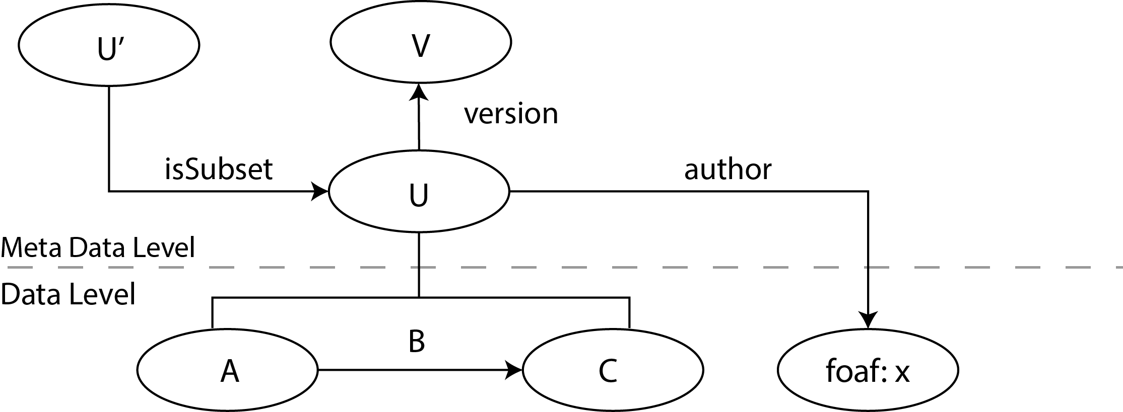
Figure 1: An example of well-stratified data.

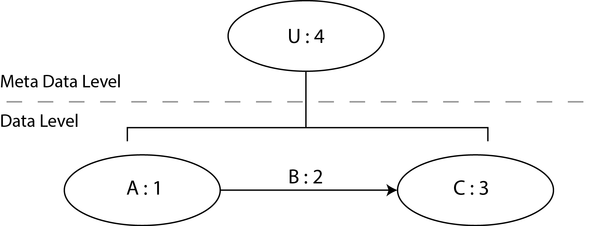
Figure 2: An example of meta-information levels assignment.

5.   Towards a Well-Stratified data language

In the previous sections we introduced the concept of well-stratified data, that is crucial to the practical realisation of data citation: as long as data is well-stratified resolving a data citation is always possible. Moreover we showed how assessing the well-stratification of a data set is linear with respect to the size of the data and can be done incrementally as new statements are added to the data set. In this section we discuss how these notions may translate into practice.

Intuitively, for a data set to be well-stratified it means that it is always possible to draw a line separating information from meta-information while baring in mind that such separation is bound to be inherently relative to current datum. In order to illustrate this idea consider the simple example depicted in Figure 1: the triple $(A,B,C)$ is the information, while its identifier $U$ and its related predicates represent the meta-information with respect to the datum considered i.e. $(A,B,C)$. Intuitively $U$ is the IRI of the reified statement that has as subject, object, and predicate respectively $A$, $C$, and $B$. Each IRI in the data set should belong to exactly one of these levels. Theoretically, there should be no upper bound to the number of meta-information levels since one might be interested in expressing statements over meta-information. An hypothetical reification, for instance, of $(U,\mathtt{version},V)$ having as identifier $I$ would imply a further meta-information level containing only $I$.

This intuitive stratification can be seen as assigning to (meta-)information to levels that decreases as we move from meta-information to information. The lowest level contains all the data that data citation resolution should ultimately reach. Well-stratification not only ensures the existence of a lowest level but it also guarantees that wherever a reasoner starts unravelling the (meta-)information chain it will eventually reach said level.

Indeed this is the approach described in Section 4 and embodied by the function $\Gamma\colon V\rightharpoonup\mathbb{N}$ used by the type system introduced in Section 4.3. From a concrete perspective this means that identifiers of a reified statement should therefore be assigned a higher level by $\Gamma$ than their subject, object, and predicate. This condition is met if, and only if, the data set is well-stratified. Finally, we remark that finding such levels can be done incrementally while reading the data set or on-the-fly as operations are performed on a well-stratified set; the cost of the former is linear in the size of the base whereas the cost of the second is linear on the number of operations.

The various data levels that can be identified this way can be considered as distinct data “slices” that, though linked, can be considered independent data sets and treated accordingly. For instance a large, multi-layered data set could be distributed as a whole, with all layers of meta-information or “reduced” to its sole data level, i.e., without meta-information. Since well-stratification can be checked automatically in a reasonably efficient way and allows the separation of meta-information from ground level information, it addresses the need for such a separation introduced by state of the art data citation methodologies [25]. Such a concept, however, does not exist yet in the Semantic Web stack. The RDF language in fact has several limitations that make well-stratification hard to realise, and here we pinpoint the most evident:

• Checking well-stratification implies, as shown in Section 4.3, the presence of a type-checking mechanism that does not exist in RDF.

• There is a data-level usage of reification (for instance to express sentences like “Bob says that Alice is kind”) that must not be confused with the labelling of triples for meta-information expression purpose we analysed so far, and RDF does not provide a way to discriminate them.

• Assigning an identifier to a triple in RDF is not handy due to the bloated syntax of reification.

To overcome these limitations we strongly advocate the creation of a new language wherein the concept of well-stratification is a first-class citizen. More specifically, such a language should include in its specifications:

• a class for meta-information objects, allowing to explicitly state which triples are to be considered meta-information and which information;

• a level property that can be associated to any IRI, serving as explicit annotation of the information level the IRI belongs to;

• a syntax for quad semantics, i.e., switching from a language of triples (like RDF) to a language of quadruples where triples are considered quadruples with a void fourth element;

• a more restrictive semantics for the fourth element of the quadruple, allowing to discriminate between reification for meta-information annotation purpose from actual data level usage;

• a type system for data including well-stratified data.

Given such a language the actual information would be still expressed in the form of triples, allowing compatibility with the other levels of the Semantic Web, and the meta-information could be handled separately.

6.   Conclusions

In this paper we briefly outlined a formalisation of data citation over linked data and showed how resolving authorship attribution, subset and version identification are computable in an efficient way as long as the considered data is well-stratified. Because of the relevance of this property, we explored how it can be expressed and verified by means of a type system and ad hoc algorithms. We showed that checking whether a given NG family (which abstracts over the concrete form of data) is well-stratified requires linear time and proposed a constant time solution for checking if an operation performed by any reasoner preserves or breaks this property.

With respect to the problem of data citation, the expressive power of OWL and RDF is largely over-abundant and might be harmful since a misuse of their primitives might break the stratification of information and meta-information, thus making resolving citations an undecidable problem. In our opinion, a more restricted language, designed specifically to grant the stratification of data should be taken into consideration to effectively enable problems such as data citation and provenance assessment to be resolved in practical time, allowing the creation of an effective data trust layer. Attaching meta-information to data published on the Web leveraging such a language might be, in our opinion, Linked Open Data’s sixth star, like publishing versioned code is a fundamental quality requirement for Open Source software. The similarity between data meta-information handling and source code versioning is striking since they address similar problems: tracking who and how edited something, identifying subsets of the managed items, and allowing external application or documents to refer to a specific revision. In our opinion this separation is also consistent with the present development of the Semantic Web stack: OWL itself, thought being a logical extension of RDFS, is not built on the top of RDFS but is rather a distinct language sharing concepts and primitives with RDFS. In a similar way a new language for data meta-information management could be built compatibly with RDF and the Linked Data philosophy without being RDF.

Finally, this work suggests a deeper connection between formal graph models and knowledge management problems encountered by the Digital Libraries and Semantic Web communities. In our opinion a more formal take on a broad range of non trivial knowledge management tasks and practises might provide relevant insights both on the application side and on the theoretical one as suggested by preliminary works in this directions like e.g. [27, 17, 18, 20].

References

• [1]
• [2] K. Alexander, R. Cyganiak, M. Hausenblas, and J. Zhao. Describing linked datasets with the void vocabulary, 2011. W3C interest group note.
• [3] M. Altman, C. Borgman, M. Crosas, and M. Matone. An introduction to the joint principles for data citation. Bulletin of the American Society for Information Science and Technology, 41(3):43–45, 2015.
• [4] M. Altman and M. Crosas. The evolution of data citation: From principles to implementation. IAssist Quarterly, 63, 2013.
• [5] S. Anam, B. H. Kang, Y. S. Kim, and Q. Liu. Linked data provenance: State of the art and challenges. In Proceedings of the 3rd Australasian Web Conference (AWC 2015), volume 27, page 30, 2015.
• [6] R. Bruni, A. Corradini, F. Gadducci, A. Lluch-Lafuente, and U. Montanari. On gs-monoidal theories for graphs with nesting. In G. Engels, C. Lewerentz, W. Schäfer, A. Schürr, and B. Westfechtel, editors, Graph Transformations and Model-Driven Engineering - Essays Dedicated to Manfred Nagl on the Occasion of his 65th Birthday, volume 5765 of Lecture Notes in Computer Science, pages 59–86. Springer, 2010.
• [7] P. Buneman, S. Khanna, and T. Wang-Chiew. Why and where: A characterization of data provenance. In Database Theory—ICDT 2001, pages 316–330. Springer, 2001.
• [8] J. J. Carroll, C. Bizer, P. Hayes, and P. Stickler. Named graphs, provenance and trust. In Proceedings of the 14th international conference on World Wide Web, pages 613–622. ACM, 2005.
• [9] G. Ciobanu, R. Horne, and V. Sassone. Minimal type inference for linked data consumers. Journal of Logical and Algebraic Methods in Programming, 2014.
• [10] G. Engels and A. Schürr. Encapsulated hierarchical graphs, graph types, and meta types. Electronic Notes in Theoretical Computer Science, 2:101 – 109, 1995. SEGRAGRA.
• [11] P. Hayes and B. McBride. Rdf semantics, 2004.
• [12] T. Heath and C. Bizer. Linked data: Evolving the web into a global data space. Synthesis lectures on the semantic web: theory and technology, 1(1):1–136, 2011.
• [13] I. Horrocks, P. F. Patel-Schneider, and F. Van Harmelen. From shiq and rdf to owl: The making of a web ontology language. Web semantics: science, services and agents on the World Wide Web, 1(1):7–26, 2003.
• [14] B. Klin and V. Sassone. Structural operational semantics for stochastic and weighted transition systems. Information and Computation, 2013.
• [15] G. Klyne, J. J. Carrol, and B. Mc Bride. Rdf 1.1 concepts and abstract syntax, 2014.
• [16] D. De Nart, D. Degl’Innocenti, M. Peressotti, and C. Tasso. Stratifying semantic data for citation and trust: An introduction to RDFDF. In M. Agosti, M. Bertini, S. Ferilli, S. Marinai, and N. Orio, editors, Proc. IRCDL, volume 701 of Communications in Computer and Information Science, pages 104–111, 2016.
• [17] A. Mansutti, M. Miculan, and M. Peressotti. Distributed execution of bigraphical reactive systems. ECEASST, 71, 2014.
• [18] A. Mansutti, M. Miculan, and M. Peressotti. Multi-agent systems design and prototyping with bigraphical reactive systems. In K. Magoutis and P. Pietzuch, editors, Proc. DAIS, volume 8460 of Lecture Notes in Computer Science, pages 201–208. Springer, 2014.
• [19] M. Miculan and M. Peressotti. Bigraphs reloaded: a presheaf presentation. Technical Report UDMI/01/2013, Dept. of Mathematics and Computer Science, Univ. of Udine, 2013.
• [20] M. Miculan and M. Peressotti. A CSP implementation of the bigraph embedding problem. CoRR, abs/1412.1042, 2014.
• [21] M. Miculan and M. Peressotti. GSOS for non-deterministic processes with quantitative aspects. In N. Bertrand and L. Bortolussi, editors, Proc. QAPL, volume 154 of Electronic Proceedings in Theoretical Computer Science, pages 17–33. 2014.
• [22] M. Miculan and M. Peressotti. Structural operational semantics for non-deterministic processes with quantitative aspects. Theoretical Computer Science, 655:135–154, 2016.
• [23] R. Milner. The Space and Motion of Communicating Agents. Cambridge University Press, 2009.
• [24] T. Omitola, N. Gibbins, and N. Shadbolt. Provenance in linked data integration. In Future Internet Assembly, pages 16–17. Ghent, Belgium, 2010.
• [25] G. Silvello. A methodology for citing linked open data subsets. D-Lib Magazine, 21(1):6, 2015.
• [26] Y. L. Simmhan, B. Plale, and D. Gannon. A survey of data provenance techniques. Computer Science Department, Indiana University, Bloomington IN, 47405, 2005.
• [27] W. Wang and T. T. Hildebrandt. Dynamic ontologies and semantic web rules as bigraphical reactive systems. In E. Tuosto and C. Ouyang, editors, Proc. WS-FM, volume 8379 of Lecture Notes in Computer Science, pages 127–146. Springer, 2013.
• [28] M. Wylot, P. Cudre-Mauroux, and P. Groth. Tripleprov: Efficient processing of lineage queries in a native rdf store. In Proceedings of the 23rd International Conference on World Wide Web, WWW ’14, pages 455–466, New York, NY, USA, 2014. ACM.
• [29] A. Zimmermann, M. Krötzsch, J. Euzenat, and P. Hitzler. Formalizing ontology alignment and its operations with category theory. In Proc. 4th International conference on Formal ontology in information systems (FOIS), pages 277–288. IOS Press, 2006.