Where You Are Is Who You Are: User Identification by Matching Statistics

Abstract

Most users of online services have unique behavioral or usage patterns. These behavioral patterns can be exploited to identify and track users by using only the observed patterns in the behavior. We study the task of identifying users from statistics of their behavioral patterns. Specifically, we focus on the setting in which we are given histograms of users’ data collected during two different experiments. We assume that, in the first dataset, the users’ identities are anonymized or hidden and that, in the second dataset, their identities are known. We study the task of identifying the users by matching the histograms of their data in the first dataset with the histograms from the second dataset. In recent works [1, 2] the optimal algorithm for this user identification task is introduced. In this paper, we evaluate the effectiveness of this method on three different types of datasets with up to $50,000$ users, and in multiple scenarios. Using datasets such as call data records, web browsing histories, and GPS trajectories, we demonstrate that a large fraction of users can be easily identified given only histograms of their data; hence these histograms can act as users’ fingerprints. We also verify that simultaneous identification of users achieves better performance compared to one-by-one user identification. Furthermore, we show that using the optimal method for identification indeed gives higher identification accuracy than heuristics-based approaches in practical scenarios. The accuracy obtained under this optimal method can thus be used to quantify the maximum level of user identification that is possible in such settings. We show that the key factors affecting the accuracy of the optimal identification algorithm are the duration of the data collection, the number of users in the anonymized dataset, and the resolution of the dataset. We also analyze the effectiveness of $k$-anonymization in resisting user identification attacks on these datasets.

I Introduction

A common task in data analysis is to identify users by exploiting statistics of their data. In many applications, we have access to some information about a set of users from one source, and some other information about the set of users from another source, and the task is to match pieces of information from the first source to pieces of information from the second source that correspond to the same underlying user. If the identities of the users in the two sets are known, then this is a trivial task. However, in many practical applications, the identities of the users are unknown either in the first set or in the second set or in both; therefore, in such cases, the task becomes non-trivial. For example, the two datasets might contain information about location statistics of users in a city measured over distinct time periods. The first set can be obtained by tracking cell phone connections to cell-towers and the second set can be obtained from credit-card usage patterns. In this case, the task is to identify the correct matching from the users’ phone numbers to their credit card numbers. Another example of the matching problem is relevant to datasets collected from the same service during two different time periods. For instance, the users on a website might choose to change their online user identities for privacy purposes; but given the statistics of the users’ data measured prior to the change and after the change, it might still be possible to identify the users by matching the statistics across the two time periods. Matching users between two datasets increases the net information available about the users, which in turn is useful for providing better targeted advertisements and recommendations for products and services [3].

The problem of matching users is also relevant in the context of privacy of an anonymized database. In recent years, many datasets containing information about individuals have been released into the public domain in order to provide open access to statistics or to facilitate data-mining research. Often these databases are anonymized by suppressing identifiers that reveal the identities of the users, such as names or social security numbers. Nevertheless, recent research has revealed that the privacy offered by such anonymized databases could be compromised, if an adversary correlates the revealed information with auxiliary information about the users from publicly available databases. A famous example of such a de-anonymization attack was shown in [4], in which anonymous movie ratings released during the Netflix Prize contest were de-anonymized by using public user reviews from the Internet Movie Database (IMDB). In such attacks, the adversary’s task of de-anonymization is essentially a matching task. The objective is to identify users in the anonymized dataset by matching their data to the publicly available auxiliary information.

As the question of matching users is relevant in many applications, this problem has been studied by many authors in different fields, including database management [5], information retrieval [6], natural language processing [7], author identification [8, 9], and privacy  [4]. Nevertheless, most solutions to the matching problem rely on heuristics that are relevant for specific applications, but not for other applications. In this paper, we present a systematic study of the matching problem under a general setting. The problem we study differs from typical approaches in data analysis in that we focus on the setting in which the available information about a user’s data is in the form of histograms of the user’s data. The histograms capture the habits of the users. In the case of mobility traces, such histograms could be the average time spent by each user at different locations during a day, or during different time intervals. In some applications, such as urban planning, the data collected naturally contains only the statistics of the data, as they are sufficient for such applications. In other applications, the data is intentionally stripped of timing information to enhance the privacy of the users; in which case, all that remains are histograms. We study the problem of matching histograms of users’ data measured in two independent experiments as a hypothesis testing problem. This novel formulation has the advantage of making it possible to rigorously define the accuracy of a matching scheme and to identify an algorithm that is provably more accurate than other schemes.

An example of a user identification task, is to consider a dataset comprised of unlabeled location histograms, given in Table II(a), where the user identities are removed. Now consider an adversary who has access to the labeled location histograms of the same users in an independent experiment where the user identities are known (refer to Table II(b)). This information could be obtained, for instance, by tracking the users during a different time-period compared to those in Table II(a). The histograms corresponding to each user in the two tables are expected to be similar, as the habits of the user are expected to remain the same across the two datasets; but they might not be exactly identical due to the inherent randomness in the user’s behavior. The objective of the adversary is to match the user identities (i.e., the rows) across the two tables.

​​User​​	Location
	​​Dorm.​​	​​Rest.​​	​​Lib.​​
?	$75\%$	$15\%$	$10\%$
?	$31\%$	$30\%$	$39\%$
?	$15\%$	$15\%$	$70\%$
?	$15\%$	$65\%$	$20\%$

(a) Unlabeled histograms (Day $1$)

​​User​​	Location
	​​Dorm.​​	​​Rest.​​	​​Lib.​​
John	$33\%$	$33\%$	$34\%$
Jill	$70\%$	$20\%$	$10\%$
Mary	$15\%$	$60\%$	$25\%$
Mike	$15\%$	$20\%$	$65\%$

(b) Labeled histograms (Day $2$)

TABLE I: An illustrative example of user identification task on histograms. Location statistics in the form of histograms of some users are released (in (a)), where the user identities are removed. An adversary has access to some auxiliary histograms (in (b)) about the same users where the user identities are known. The time period during which the histograms in (a) are collected does not overlap with the time period during which the histograms in (b) are collected. The objective of the adversary is to match the users (i.e., rows) across the two tables.

In the next section, we provide a detailed comparison of this problem with existing literature on user identification and highlight the new contributions of this work. We state the problem in mathematical form and propose our solution in Section III. We experimentally evaluate our solution by using three different datasets in Section IV. In Section V, we analyze the efficacy of our algorithm if additional privacy enhancing techniques, such as $k$-anonymization, are applied to histograms of users’ data. We conclude the paper with some discussions in Section VI.

II Related work and contributions

The user matching studied in this paper is closely related to several problems that have been studied in other different communities. In this section, we present a comparison of our approach with related problems from several areas, and highlight our contributions relative to existing work.

II-A Entity resolution

A matching problem studied in the database community is that of identifying different data records that refer to the same real-world object [5]. Similarly, in natural-language processing, the problem of linking different mentions of the same underlying entity in text [7] is analogous to the objective in the user-matching problem. Another example from the information-retrieval literature is the problem of classifying documents by their authors, given documents from different authors with the same name [6]. User matching has also been studied in the social-networks community in which the objective is to identify different profiles that belong to the same underlying user [10]. Such problems fall under the umbrella-term entity resolution (ER) [11]. In these problems, the available information about the users is often not in the form of histograms, and the solutions proposed are often based on heuristics and practical convenience; whereas the solution we propose in this paper is specific to the setting in which the only information available about the users is in the form of histograms, and in this setting, the solution is optimal for minimizing the probability of misclassification.

II-B De-anonymization attacks

Our work is also closely related to the literature on de-anonymization methods [4],[12] studied in the literature on privacy. A number of works on de-anonymization focus on demonstrating that even when users’ data are anonymized, the data belonging to each user is often unique. In such examples, an adversary who has access to auxiliary information about the users can de-anonymize the anonymized datasets by exploiting the uniqueness of the data belonging to each user. For example, in [13] the authors perform a study on the top $k$ locations most frequently visited by users in a nationwide call-data record (CDR) dataset. They consider various levels of spatial granularity (such as sector, cell, zip code, city, state, and country) and temporal granularity (such as day and month), and they show that the most frequently visited locations can act as quasi-identifiers to re-identify anonymous users. Thus an adversary can de-anonymize such a dataset by obtaining access to auxiliary information about the users’ zip codes and times of activity. The adversary’s goal is essentially a matching task, i.e., the adversary seeks to match the auxiliary information about the users with the unique aspects of the users’ data. Some other works such as [14, 15, 16, 17, 18, 13, 19] study the uniqueness of mobility data traces. There is a line of work on studying the uniqueness of web browsing history patterns of users [20, 21]. In [20] the authors consider a dataset where every record is the set of visited websites by a user during some period of time. The authors investigate how unique is a single user’s record compared to other users’ records in the dataset.

Although our work is related to de-anonymization, it differs in several aspects. First, we assume that the only information about the users in the two datasets are time-averaged statistics of the users’ data. In most works on user matching and de-anonymization [4, 22, 23], the vulnerability to privacy breaches often arises due to the sparsity of the temporal evolution of the users’ data. For instance, the fact that a user watched and rated a movie during a particular time-period or was at a specific location during a particular time can be used to easily identify the user’s data from the anonymized dataset. Other de-anonymization works focus on identifying the temporal patterns of the data collected from the users. For example, in [17, 18], a Markov model is constructed based on the temporal evolution of the mobility patterns of the users, and then similarity measures are used for de-anonymization. Such temporal information in the users’ data, however, is removed when only statistics in the form of histograms from each user is collected or released. Often this results in a much lower uniqueness in the information available about the users; hence matching users’ statistics is, in general, much more difficult than matching users’ datasets.

Second, we assume that the two sets of the statistical information are mutually statistically independent. For example, in the case of mobility data, this could be because the two datasets were obtained over different time periods. We seek to perform the matching by only exploiting the fact that users’ habits remain stationary and ergodic across the two datasets. This is in contrast to the approach of works such as [15, 24, 16] that perform de-anonymization by using auxiliary information collected over the same period of time as the anonymized dataset. In such cases, the auxiliary information is not independent of the anonymized user data. In [20], the authors investigate the stability of the set of visited websites by a user across time. In particular, they record the set of visited websites by a user during one day. They use the Jaccard index to measure the similarity between the sets collected for one user over different days. They show that the set of visited websites by a user is stable during a four-week period. A special case of our work is when the labeled and unlabeled histograms are obtained from the same source in different time periods. The accuracy of our matching algorithm in such cases is dependent on how how much the statistical characteristics of the data is preserved over time.

Third, we perform simultaneous matching of the information available about all users and not one user at a time. Simultaneous matching takes into account all the information available about the users at the same time, and hence outperforms matching users one at a time. Simultaneously taking into account all the information for various attacks has already been employed in different domains [25, 9, 26, 27] and in this paper we employ it in the domain of histogram matching.

There is also a related line of work on graph de-anonymization, also known as graph alignment [28, 22, 23]. It is the problem of matching the nodes across two similar graphs, where the only available information is the two graphs. For example, given the graph of connections between users on two different social networks (e.g., Facebook and LinkedIn), it might be possible to match users across the two social networks by exploiting the fact that the structure of the underlying graphs are expected to be similar. This problem is different from that studied in the present paper because, in our setting, the graph-based connections among the users are not available.

II-C Supervised learning

The matching task studied in this paper is closely related to the classification task studied in supervised learning [29], where the objective is to classify test data to the correct class based on labeled training data observed under each of the classes. Nevertheless, a key aspect of our approach that differs from supervised learning is that we seek to simultaneously classify test data that belong to a group of users subject to the constraint that each user belongs to a distinct class (refer to Figure 1). Thus our solution, originally introduced in [1, 2], can be interpreted as a solution to a constrained classification problem. Our solution is tailored to the setting in which the available information is in the form of histograms. It could be possible to extend this solution to more general kinds of data by combining the matching algorithm presented in this work with feature extraction techniques in machine learning [29].

\psfrag{S}[l][Bc]{\parbox[c]{39.83368pt}{\begin{center} Training \\ histograms\end{center}}}\psfrag{U}[r][Bc]{\parbox[c]{34.14322pt}{\begin{center} Test \\ histogram \end{center}}}\includegraphics[width=195.12767pt]{histMatching.eps}

(a) Histogram classification

\psfrag{S}[l][Bc]{\parbox[c]{39.83368pt}{\begin{center} Training \\ histograms\end{center}}}\psfrag{U}[r][Bc]{\parbox[c]{39.83368pt}{\begin{center} Test \\ histograms \end{center}}}\includegraphics[width=195.12767pt]{histClassification.eps}

(b) Histogram matching

Figure 1: (a) The problem of histogram classification, which is to to classify the test histogram to the correct class based on the training histograms. (b) The problem of histogram matching studied in this paper, which is to simultaneously classify the test histograms to the training histograms subject to the constraint that each test histogram belongs to a distinct class.

II-D Contributions

Compared to existing works on the user-matching problem, our work is unique in several respects. Our main contributions can be summarized as follows:

• We demonstrate that statistics about users’ behaviors contain a significant amount of information that can be used as fingerprints to uniquely identify users, by an adversary who has access to auxiliary information about the users. Moreover, we show that identification by using only data statistics can sometimes result in accuracy higher than existing methods based on more complicated data models (e.g., Markov Chains).

• We evaluate a provably optimal algorithm for matching users’ statistics on three datasets of diverse nature and demonstrate that it outperforms heuristics-based methods. We address the practical setting of performing the matching across distinct sets of users.

• We compare the performance of our algorithm with different parameters and under different settings, such as user configuration and data resolution. We verify that, in particular, matching users simultaneously leads to a matching accuracy significantly higher than matching one user at a time.

• We analyze the performance of the matching algorithm under different privacy-preserving mechanisms such as data obfuscation and $k$-anonymization.

III Problem Statement and Proposed Solution

We assume that the data belonging to each user in our system follows some fixed underlying probability law that is unknown a priori. The probability law associated with each user is unique and captures the habits of the user. For example, in the case of web-browsing histories, the probability law captures the user’s relative preferences for various websites. Similarly, in the case of shopping data, the probability law could represent shopping preferences and, in the case of mobility data, the law could represent the preferences for visiting various locations. In the basic version of the user-matching problem, we are given two datasets corresponding to the same set of users, and the task is to match users across the two datasets by exploiting the fact that the underlying probability law of each user is unique. We will later generalize this to the setting in which the two datasets belong to different sets of users. Throughout this paper, we focus on the specific setting in which each dataset reveals only the histograms of each user’s data and not the data itself. We use the term adversary to denote the entity that performs the user-matching task. We use feminine pronouns for referring to the users and masculine pronoun for referring to the adversary. In the following, we state the problem mathematically.

III-A Problem statement

Consider a discrete alphabet set $\mathcal{S}=\{S_{1},S_{2},\ldots,S_{K}\}$ of size $|\mathcal{S}|=K$ and a set of $N$ users labeled $1,2,\ldots,N$. The set $\mathcal{S}$ represents the set of all possible values that can be taken by each instance of the data belonging to each user. For example, in the case of web-browsing data, $\mathcal{S}$ is the set of all websites that a user could visit, and in the case of mobility data, $\mathcal{S}$ is the set of all possible locations (e.g., regions of a city) that a user could visit. For the purpose of illustration, in the rest of this section, we will focus on the example of mobility data.

For a data string $s=[s(1),s(2),\ldots,s(T)]\in\mathcal{S}^{T}$ of length $T$, we use $\Gamma_{s}$ to denote the histogram (i.e., empirical distribution) of the string defined as

$$\Gamma_{s}(l)=\frac{1}{T}\sum_{t=1}^{T}{\cal I}\{s(t)=S_{l}\},\;l=1,2,\ldots,K.$$ (1)

In the simplest version of the user-matching problem studied in this paper, we are given two sets of histograms of the data generated by each of the users. Let set $\psi_{1}=\{\Gamma_{x_{1}},\Gamma_{x_{2}},\ldots,\Gamma_{x_{N}}\}$ represent a set of unlabeled histograms each generated by a distinct user, and let $\psi_{2}=\{\Gamma_{y_{1}},\Gamma_{y_{2}},\ldots,\Gamma_{y_{N}}\}$ represent a set of labeled histograms each generated by a distinct user. Here $\psi_{1}$ and $\psi_{2}$ represent the histograms contained in two datasets. In the case of mobility data, $\psi_{1}$ is a set of anonymized histograms of users’ mobility traces that are released, and $\psi_{2}$ represents the auxiliary histograms of the users’ mobility traces, which is obtained by an adversary by tracking the users over a time period. In other applications, the auxiliary histograms can be obtained by the adversary by using publicly available information. In both cases, the adversary is aware of the users’ identities in the second dataset, and seeks to decode the identities of the users in the first anonymized set of histograms. The histograms of each user are assumed to be statistically independent of those of others. Furthermore, for each user, the histogram generated by the user in the first dataset is assumed to be independent of the histogram in the second dataset. In the mobility example, independence is a reasonable assumption provided that there is no overlap between the time-periods over which the histograms in $\psi_{1}$ and $\psi_{2}$ are computed. For example, $\psi_{1}$ contains histograms collected over a week and $\psi_{2}$ contains histograms collected over the following week.

In the matching problem, the objective of the adversary is to determine the true matching between the histograms of $\psi_{1}$ and $\psi_{2}$. We represent the ground truth via an unknown permutation function,

$$\bm{\sigma}:\{1,2,\ldots,N\}\mapsto\{1,2,\ldots,N\}$$ (2)

such that, in reality, for each $i\in\{1,2,\ldots,N\}$, the histograms $\Gamma_{x_{\bm{\sigma}(i)}}$ and $\Gamma_{y_{i}}$ are generated by the same user $i$. The objective in the matching problem is, equivalently, to estimate $\bm{\sigma}$. In Section III-D, we discuss the practical setting where the histograms in the sets $\psi_{1}$ and $\psi_{2}$ are generated by different sets of users.

III-B Potential approach: Weighted bipartite matching

The problem of matching histograms across two sets can be best visualized as a matching problem on a bipartite graph. Let $G=(V_{1},V_{2},E)$ be a complete bipartite graph where each vertex in the set $V_{1}$ (respectively, set $V_{2}$) is associated with a unique histogram in the set $\psi_{1}$ (respectively, set $\psi_{2}$). There exists an edge from each element in $V_{1}$ to each element in $V_{2}$ and no edges between elements in $V_{1}$ or $V_{2}$. Hence we have a complete bipartite graph where $V_{1}$ and $V_{2}$ form the two parts. Let node $j$ in set $V_{1}$ and node $i$ in set $V_{2}$ be associated with histogram $\Gamma_{x_{j}}$ in $\psi_{1}$ and $\Gamma_{y_{i}}$ in $\psi_{2}$, respectively. The graph $G$ is illustrated in Figure 2.

\psfrag{x}[Bc][Bc]{\small{$\Gamma_{x_{1}}$}}\psfrag{a}[Bc][Bc]{\small{$\Gamma_{x_{2}}$}}\psfrag{b}[Bc][Bc]{\small{$\Gamma_{x_{N}}$}}\psfrag{y}[Bc][Bc]{\small{$\Gamma_{y_{1}}$}}\psfrag{c}[Bc][Bc]{\small{$\Gamma_{y_{2}}$}}\psfrag{d}[Bc][Bc]{\small{$\Gamma_{y_{N}}$}}\psfrag{w}[Bc][Bc]{\small{$w_{11}$}}\psfrag{S}[Bc][l]{\parbox[c]{85.35826pt}{\begin{center} Dataset one \\ histograms ($\psi_{1}$)\end{center}}}\psfrag{U}[Bc][l]{\parbox[c]{85.35826pt}{\begin{center} Dataset two \\ histograms ($\psi_{2}$)\end{center}}}\includegraphics[width=216.81pt]{bipartiteMatching.eps}

Figure 2: The problem of matching histograms across two sets can be visualized as a matching problem on a weighted bipartite graph. Corresponding to the $N!$ different permutations, there are $N!$ possible maximal matchings on $G$. The green edges represents the correct matching associated with $\bm{\sigma}$ in (2). The solution can be obtained via a weighted bipartite matching algorithm on the graph with appropriate edge weights.

A matching in graph $G$ is a subset of edges $E$ of $G$ such that no two edges in the subset share a vertex. A maximal matching is a matching such that the addition of any edge to the subset violates the matching property. Let $\bm{\sigma}_{m}$ be a permutation of $\{1,2,\ldots,N\}$, for $m=1,2,\ldots,N!$. There are $N!$ possible maximal matchings on $G$ corresponding to the $N!$ different permutations. The matching corresponding to permutation $\sigma_{m}$ is the matching in which each node $i$ from set $V_{2}$ is mapped to node $\bm{\sigma}_{m}(i)$ in $V_{1}$; in other words, histogram $\Gamma_{y_{i}}$ in $\psi_{2}$ is mapped to histogram $\Gamma_{x_{\bm{\sigma}_{m}(i)}}$ in $\psi_{1}$. The matching associated with $\bm{\sigma}$ in (2) is shown by green edges in Figure 2.

An intuitive approach for estimating the correct matching between the histograms is as follows. Define a weight for every edge in $G$ such that the weight of the edge $w_{ji}$ from $j$ to $i$ is equal to some appropriately defined distance between the histograms $\Gamma_{x_{j}}$ and $\Gamma_{y_{i}}$, i.e.,

$$w_{ji}=\mbox{d}(\Gamma_{x_{j}},\Gamma_{y_{i}})$$ (3)

for some distance measure $\mbox{d}(.)$. Now perform a minimum-weight maximal bipartite matching on the resultant weighted bipartite graph. The minimum-weight maximal matching corresponds to a configuration where the sum of the distances between the matched histograms is minimum, hence expected to provide a good estimate for the correct matching.

The relevant questions that arise here are: What is a good choice for the distance measure between histograms and does the choice of measure depend on the nature of the data or can there be a general-purpose measure? The literature contains various choices of prevalent distance measures that can be used in the weight function. For example, in [13] the authors use the cosine distance between the histograms of the number of calls of users at different GSM antennas as a distance measure for analyzing the call behavior of users. The cosine distance between histograms $\Gamma_{x_{j}}$ and $\Gamma_{y_{i}}$ is defines as

$$w_{ji}^{\mbox{cos}}=1-\frac{\left<\Gamma_{x_{j}},\Gamma_{y_{i}}\right>}{\left\|\Gamma_{x_{j}}\right\|_{2}\left\|\Gamma_{y_{i}}\right\|_{2}},$$ (4)

where $\left<\Gamma_{x_{j}},\Gamma_{y_{i}}\right>$ is the dot product between the histograms, which we denote by $w_{ji}^{\mbox{dot}}$,

$$w_{ji}^{\mbox{dot}}=\left<\Gamma_{x_{j}},\Gamma_{y_{i}}\right>=\sum_{l=1}^{K}\Gamma_{x_{j}}(l)\Gamma_{y_{i}}(l),$$ (5)

and $\left\|\Gamma_{s}\right\|_{2}=\sqrt{\sum_{l=1}^{K}{\Gamma_{s}(l)}^{2}}$. Another heuristic measure often used in the machine learning community is the $l_{1}$ distance between the histograms, given by

$$w_{ji}^{l_{1}}=\left\|\Gamma_{x_{j}}-\Gamma_{y_{i}}\right\|_{1}=\sum_{l=1}^{K}\left|\Gamma_{x_{j}}(l)-\Gamma_{y_{i}}(l)\right|.$$ (6)

Alternatively, we can use a similarity measure, such as the dot product defined in (5) as the weight function in (3). We then identify the best permutation by using a maximum weight matching on the resultant weighted bipartite graph. In the next subsection, we present a new choice of the weight function and argue that it is a judicious choice.

III-C Optimal solution via hypothesis testing interpretation

The problem of finding the matching between the histograms of $\psi_{1}$ and $\psi_{2}$ can be viewed as a multi-hypothesis testing problem with $N!$ hypotheses, $\{H_{1},H_{2},\ldots,H_{N!}\}$, where hypothesis $H_{m}$ corresponds to permutation $\sigma_{m}$, for $m=1,2,\ldots,N!$. In the hypothesis testing framework, we study decision rules by using probability of error under the different hypotheses as the performance metric. Typical solutions to hypothesis testing problems seek the decision rule that leads to an optimal trade off between various error probabilities under the different hypotheses. In our prior works [1, 2], we showed that, when each user’s data is generated by an i.i.d. process governed by her probability law, an optimal trade-off between the various error probabilities for the matching problem is obtained by deciding in favor of the hypothesis corresponding to the minimum-weight maximal matching on the bipartite graph $G$ with edge weights

$$w_{ji}=D(\Gamma_{x_{j}}\|{\mathchoice{\genfrac{}{}{}{1}{1}{2}}{\genfrac{}{}{}{1}{1}{2}}{\genfrac{}{}{}{3}{1}{2}}{\genfrac{}{}{}{3}{1}{2}}}({\Gamma_{x_{j}}+\Gamma_{y_{i}}}))+D(\Gamma_{y_{i}}\|{\mathchoice{\genfrac{}{}{}{1}{1}{2}}{\genfrac{}{}{}{1}{1}{2}}{\genfrac{}{}{}{3}{1}{2}}{\genfrac{}{}{}{3}{1}{2}}}({\Gamma_{x_{j}}+\Gamma_{y_{i}}})).$$ (7)

In (7), $D(\cdot\|\cdot)$ is the Kullback-Leibler divergence function [30], defined as

$$D(\pi\|\mu)=\sum_{l=1}^{K}\pi(l)\log\left(\pi(l)/\mu(l)\right).$$

The weight $w_{ji}$ in (7) satisfies $0\leq w_{ji}\leq 2\log(2)$ and it is equal to $0$ when $\Gamma_{x_{j}}=\Gamma_{y_{i}}$ and equal to $2\log(2)$ when the histograms have disjoint support (i.e., when $\nexists\;l$ such that $\Gamma_{x_{j}}(l),\Gamma_{y_{i}}(l)>0$). The exact optimality result is based on an asymptotic analysis of error probabilities as the length $T$ of the data strings increases to infinity. It is shown in [1, 2] that a variant of this test yields optimal trade-offs between the error exponents under the different hypotheses. For the sake of completeness, we provide the intuition behind the choice of the metric (7) in the following setting. To every user $i$, we associate a probability distribution $\bm{\pi}_{i}\in\mathcal{P}_{K-1}$. The probability distributions are distinct, which means that $\bm{\pi}_{i}\neq\bm{\pi}_{m}$ for $i\neq m$, but they are unknown. Suppose that each user $i$ generates data in an i.i.d. manner from the distribution $\bm{\pi}_{i}$. Consider a set $\psi_{1}=\{x_{1},x_{2},\ldots,x_{N}\}$ of unlabeled strings of length $T$ each generated by a distinct user, and an independent set $\psi_{2}=\{y_{1},y_{2},\ldots,y_{N}\}$ of labeled strings of length $T$ each generated by a distinct user. Let $i$ denote the user who generated strings $x_{\bm{\sigma}(i)}\in\mathcal{S}^{T}$ and $y_{i}\in\mathcal{S}^{T}$ where $\bm{\sigma}$ is given in (2).

A commonly used solution for multi-hypothesis testing problems is to identify the maximum-likelihood (ML) hypothesis, which is the hypothesis under which the log-likelihood of the observations is maximized. In our problem, however, the underlying probability distributions $\bm{\pi}_{i}$’s of the users are unknown, thus the log-likelihood has to be replaced with the generalized log-likelihood. The first step is therefore to compute the generalized log-likelihood. For hypothesis $H_{m}$ the generalized likelihood is obtained by maximizing the likelihood function over all possible choices of the $\bm{\pi}_{i}$’s, and is given by

$$\mathcal{L}(H_{m})=\sup_{\bm{\pi}_{1},\bm{\pi}_{2},\ldots,\bm{\pi}_{N}}\sum_{i=1}^{N}\sum_{t=1}^{T}\Big{[} \log\left(\pi_{i}(x_{\bm{\sigma}_{m}(i)}(t))\right)$$

$$+\log\left(\pi_{i}(y_{i}(t))\right)\Big{]}.$$ (8)

It is known that for an i.i.d.-generated string, the maximum likelihood estimator of the underlying distribution is given by the empirical distribution of the string. Hence, it is easy to see that each of the $N$ terms in the summation (III-C) is maximized by setting $\bm{\pi}_{i}={\mathchoice{\genfrac{}{}{}{1}{1}{2}}{\genfrac{}{}{}{1}{1}{2}}{\genfrac{}{}{}{3}{1}{2}}{\genfrac{}{}{}{3}{1}{2}}}({\Gamma_{x_{\bm{\sigma}_{m}(i)}}+\Gamma_{y_{i}}})$, for $i=1,2,\ldots,N$. We can therefore rewrite (III-C) as

$$\mathcal{L}(H_{m})=-2T\sum_{i=1}^{N}\Big{\{}{\cal H}(\Gamma_{x_{\bm{\sigma}_{m}(i)}})+{\cal H}(\Gamma_{y_{i}})$$

$$\!+\!D(\Gamma_{x_{\bm{\sigma}_{m}(i)}}\|{\mathchoice{\genfrac{}{}{}{1}{1}{2}}{\genfrac{}{}{}{1}{1}{2}}{\genfrac{}{}{}{3}{1}{2}}{\genfrac{}{}{}{3}{1}{2}}}({\Gamma_{x_{\bm{\sigma}_{m}(i)}}\!+\!\Gamma_{y_{i}}}))\!+\!D(\Gamma_{y_{i}}\|{\mathchoice{\genfrac{}{}{}{1}{1}{2}}{\genfrac{}{}{}{1}{1}{2}}{\genfrac{}{}{}{3}{1}{2}}{\genfrac{}{}{}{3}{1}{2}}}({\Gamma_{x_{\bm{\sigma}_{m}(i)}}\!+\!\Gamma_{y_{i}}}))\Big{\}},$$ (9)

where ${\cal H}(.)$ is the Shannon entropy function [30], defined as ${\cal H}(\bm{\pi})=-\sum_{l=1}^{K}\pi(l)\log\left(\pi(l)\right)$.

The maximum generalized likelihood solution is given by $\widehat{H}=\operatorname*{arg\,max}_{H_{m}}\mathcal{L}(H_{m})$. Given the sets of histograms $\{\Gamma_{x_{j}}\}$ and $\{\Gamma_{y_{i}}\}$, the term $\sum_{i=1}^{N}{\cal H}(\Gamma_{x_{\bm{\sigma}_{m}(i)}})+{\cal H}(\Gamma_{y_{i}})$ in (III-C) is a constant term that does not depend on the hypothesis $H_{m}$. Hence, by removing this constant term we can show that $\widehat{H}=\operatorname*{arg\,min}_{H_{m}}D(H_{m})$, where $D(H_{m})=\sum_{i=1}^{N}w_{{\bm{\sigma}_{m}(i)}{i}}$ with $w_{ji}$ given in (7). Hence, $\widehat{H}$ can be interpreted as the hypothesis corresponding to the minimum-weight maximal matching on the complete bipartite graph $G$ in Figure 2 with weights (7).

Although this optimality result was established for i.i.d. processes, we argue that the solution is a reasonable approach to use for the matching problem, provided that each user’s habits follow a probability law that is stationary and ergodic. In such cases, we expect the histograms of each user in the two datasets to be similar, hence the solution for i.i.d. data is well-justified. Therefore, in this paper, we propose to use the solution given by the minimum-weight maximal matching on $G$ with the weight metric in (7). We demonstrate, in our experiments in Section IV, that the matching accuracy obtained by using (7) is indeed higher than those obtained by using (4), (5), and (6) under various settings.

III-D Generalization to different sets of distinct users

Denote by $U_{1}$ the set of users who generate the histograms $\psi_{1}$ and by $U_{2}$ the set of users who generate the histograms $\psi_{2}$. So far, we have assumed that the two sets of histograms $\psi_{1}$ and $\psi_{2}$ are generated by the same set of $N$ users; i.e., $U_{1}=U_{2}$ with $|U_{1}|=N$. In practice, however, the histograms in sets $\psi_{1}$ and $\psi_{2}$ can belong to different sets of distinct users, that is, $U_{1}\neq U_{2}$. When $U_{1}\neq U_{2}$, the adversary needs to solve the matching problem of identifying the set $U_{1}\cap U_{2}$ and of identifying the matching between the labeled and the unlabeled histograms belonging to the users in the set $U_{1}\cap U_{2}$. Our matching solution and optimality result can be extended to the case $U_{1}\neq U_{2}$ [2]. Let the number of users in sets $U_{1}$ and $U_{2}$ (i.e, number of histograms in sets $\psi_{1}$ and $\psi_{2}$) be $N$ and $N^{\prime}$, respectively. We assume that the probability law of every user in the set $U_{1}\cup U_{2}$ is distinct. Without loss of generality, we assume that $N^{\prime}>N$, i.e., there are more labeled histograms than unlabeled histograms.

First, consider the case $U_{1}\subset U_{2}$. Here $|U_{1}\cap U_{2}|=N$. It represents the scenario where for each unlabeled histogram in set $\psi_{1}$ there exists an associated labeled histogram in set $\psi_{2}$ that is generated by the same user, but not vice versa. As before we construct the complete bipartite graph $G=(V_{1},V_{2},E)$, where $|V_{1}|=N$, $|V_{2}|=N^{\prime}$, and edge weights are as in (7). The graph is illustrated in Figure 3(a). A matching between all the $N$ unlabeled histograms and $N$ out of $N^{\prime}$ of the labeled histograms is a maximal matching on the graph $G$. Similarly to the case where $U_{1}=U_{2}$, the optimal solution is given by the minimum-weight maximal matching in the graph $G$.

Now consider the more general case where $|U_{1}\cap U_{2}|=r<N$. Furthermore, let the value of $r$ be known to the adversary. This case represents the scenario where some labeled histograms in set $\psi_{2}$ are not associated with any unlabeled histograms in $\psi_{1}$ and vice versa. The graph $G$ for this case is illustrated in Figure 3(b). If the adversary knows the value of $r$, he can try to match only a set of $r$ unlabeled histograms to the labeled histograms such that the two sets are as close as possible to each other. In other words, the adversary can try to choose $r$ out of $N$ unlabeled histograms and match them to $r$ out of $N^{\prime}$ labeled histograms such that the summation of the distances between the matched pairs (given in (7)) is minimized. Such a matching can be obtained from a minimum-weight matching with cardinality $r$ on the graph $G$. This problem is also known as the minimum-cost imperfect matching [31]. We experimentally evaluate this approach in Section IV-A4. If the adversary does not know the value of $r$, he can still try to match $\min\{N,N^{\prime}\}$ users. However this leads to a larger fraction of incorrect matches, as we demonstrate in the experiments of Section IV-A4.

\psfrag{a}[Bc][Bc]{\small{$\Gamma_{x_{1}}$}}\psfrag{e}[Bc][Bc]{\small{$\Gamma_{x_{2}}$}}\psfrag{b}[Bc][Bc]{\small{$\Gamma_{x_{N}}$}}\psfrag{c}[Bc][Bc]{\small{$\Gamma_{y_{1}}$}}\psfrag{f}[Bc][Bc]{\small{$\Gamma_{y_{2}}$}}\psfrag{d}[Bc][Bc]{\small{$\Gamma_{y_{N^{\prime}}}$}}\psfrag{w}[Bc][Bc]{\small{$w_{11}$}}\psfrag{S}[Bc][Bc]{\parbox[c]{36.98866pt}{\small{\begin{center} Histograms \\ $\psi_{1}$\end{center}}}}\psfrag{U}[Bc][Bc]{\parbox[c]{36.98866pt}{\small{\begin{center} Histograms \\ $\psi_{2}$\end{center}}}}\includegraphics[width=195.12767pt]{bipartiteMatchingSubset.eps}

(a) $U_{1}\subset U_{2}$

\psfrag{a}[Bc][Bc]{\small{$\Gamma_{x_{1}}$}}\psfrag{e}[Bc][Bc]{\small{$\Gamma_{x_{2}}$}}\psfrag{b}[Bc][Bc]{\small{$\Gamma_{x_{N}}$}}\psfrag{c}[Bc][Bc]{\small{$\Gamma_{y_{1}}$}}\psfrag{f}[Bc][Bc]{\small{$\Gamma_{y_{2}}$}}\psfrag{d}[Bc][Bc]{\small{$\Gamma_{y_{N^{\prime}}}$}}\psfrag{w}[Bc][Bc]{\small{$w_{11}$}}\psfrag{S}[Bc][Bc]{\parbox[c]{36.98866pt}{\small{\begin{center} Histograms \\ $\psi_{1}$\end{center}}}}\psfrag{U}[Bc][Bc]{\parbox[c]{36.98866pt}{\small{\begin{center} Histograms \\ $\psi_{2}$\end{center}}}}\includegraphics[width=195.12767pt]{bipartiteMatchingUnC.eps}

(b) $|U_{1}\cap U_{2}|=r<N$

Figure 3: Matching problem when the histograms in sets $\psi_{1}$ and $\psi_{2}$ belong to different sets of distinct users (i.e., $U_{1}\neq U_{2}$). Histograms belonging to users in $U_{1}\cap U_{2}$ are marked by black circles and histograms in the sets $U_{1}\backslash U_{2}$ and $U_{2}\backslash U_{1}$ are marked by black triangles and squares, respectively. In (a), $U_{1}\subset U_{2}$ with $|U_{1}|=N$. The proposed solution is given by the minimum-weight maximal matching of the graph. In (b), $|U_{1}\cap U_{2}|=r<N$. In this case, the proposed solution is given by the minimum-weight matching with cardinality $r$ on the graph. The green edges represent the correct matching between the histograms in the set $U_{1}\cap U_{2}$.

III-E Algorithms and complexity

An important practical aspect of the user-matching task is the algorithm for obtaining the matching solution on the weighted graph $G$ and the associated time-complexity. In Sections III-B and III-D, we discussed three different settings for finding the matching solution between $\psi_{1}$ and $\psi_{2}$ on the graph $G$: (i) case $U_{1}=U_{2}$ depicted in Figure 2; (ii) case $U_{1}\subset U_{2}$ depicted in Figure 3(a); and (iii) the case $|U_{1}\cap U_{2}|=r<N$ depicted in Figure 3(b). We require two kinds of algorithms to identify the solutions:

• Algorithm for identifying the minimum-weight maximal matching on $G$,

• Algorithm for identifying the minimum-weight matching with a fixed cardinality $r$ on $G$.

The matching solution on $G$ can be obtained via (A1) in cases (i) and (ii), and via (A2) in case (iii). We note that in case of using a similarity measure such as (5) as the choice of the weight function in $G$, the matching solution is identified via the maximum-weight matching on $G$. In this case, after negating all the edge-weight values and shifting them to make them positive, (A1) and (A2) can be used to identify the matching solution.

The Hungarian algorithm [32] is a popular and efficient algorithm for (A1) and can be adapted to solve (A2) as explained in [31]. In our experiments, we use the Hungarian algorithm for (A1) and a polynomial-time algorithm, based on the theory of matroids (see, e.g., [33, Ch. 8]), for (A2). The time-complexity of obtaining the matching solution on the graph $G$ by using the Hungarian algorithm is $\mathcal{O}(|U_{1}||U_{2}||U_{1}\cap U_{2}|)$; i.e., it is $\mathcal{O}(N^{3})$, $\mathcal{O}(N^{2}N^{\prime})$, and $\mathcal{O}(NN^{\prime}r)$ for (i), (ii), and (iii), respectively. In practice, the complexity can often be reduced significantly. For instance, when histograms $\Gamma_{x_{j}}$ and $\Gamma_{y_{i}}$ have disjoint support, then $w_{ji}$ in (7) takes its maximum value, which is $2\log(2)$. Then the edge connecting the corresponding vertices in $G$ can be removed, as it will almost certainly not be selected in the minimum-weight maximal matching. If the resulting graph has $\mathcal{E}$ edges, then the complexity is $\mathcal{O}(\mathcal{E}|U_{1}\cap U_{2}|)$.

In a practical implementation of this de-anonymization approach, the overall complexity depends on both the complexity of computing the edge weights in graph $G$ and of running the matching algorithm (A1) or (A2) on graph $G$. The former has complexity $\mathcal{O}(NN^{\prime}K)$ where $K$ is the number of locations. In Section IV-D we present detailed time-complexity results of our de-anonymization approach.

An alternative approach for solving (A1) and (A2) is to use an approximate minimum-weight matching algorithm on graph $G$ instead of the Hungarian algorithm. Although finding the exact minimum-weight matching solution has the advantage of obtaining the maximum matching accuracy, it brings the inherent computational complexity of weighted bipartite matching into our solution. This could hinder the applicability of our solution to very large datasets as the number of histograms becomes very large. An alternative approach in dealing with very large datasets is to obtain an approximate minimum-weight matching solution on graph $G$ [34]. Although this approach reduces the matching accuracy, it makes it possible to find an approximate solution in reasonable time. For example by using the approach in [34], a $(1-\epsilon)$-approximate matching solution to (A1) in case (i) can be obtained with complexity $\mathcal{O}(N^{2}\epsilon^{-1}\log\epsilon^{-1})$ instead of $\mathcal{O}(N^{3})$.

IV Experimental Evaluations

In this section we compare the performance of the proposed matching algorithm with other methods for user identification. Although numerous identification algorithms exist in the literature, we perform comparisons primarily with identification methods that rely only on histogram information as the focus of this paper is on such methods. Nevertheless, in Section IV-C4 we compare our approach with an existing Markov-based method, for which histograms are only a subset of the information available to the method. We show that by using only histograms we can still get better de-anonymization accuracy than the Markov-based approach that exploits more information from the dataset.

We test our matching algorithms on three datasets of different nature. The first is a call-data records dataset, the second is a web browsing-history dataset, and the third is a dataset of GPS mobility traces. In our experiments, a location represents the coverage region of a GSM antenna, a website, and a region on the map in the first, second, and third dataset, respectively. We interpret the sequence of locations visited by a user as a data string. Thus a user’s histogram is simply the relative fractions of visits of the user to the different locations, within the time period considered. For each dataset, we compute the histograms of the users over two different non-overlapping time periods to obtain the sets $\psi_{1}$ and $\psi_{2}$ described in Section III-A. We then construct the complete bipartite graphs $G$ shown in Figures 2, 3(a), and 3(b) and apply the matching algorithms proposed in Sections III and III-D on this graph with appropriately chosen edge-weights. We estimate the matching accuracy obtained with the different algorithms by calculating the percentage of common users (i.e., users in the set $U_{1}\cap U_{2}$) whose histograms are correctly matched. We recall that we focus on the privacy from the perspective of the adversary and not of the users; hence, this particular choice for notion of accuracy is reasonable.

IV-A Experiments on call-data records (CDR)

IV-A1 Dataset description and preprocessing

The call-data records (CDR) dataset consists of anonymized records of phone calls between $50,000$ Orange customers (i.e., users) in Ivory Coast [35], chosen randomly from millions of users. The dataset covers the two-week period from Monday $9^{\mbox{th}}$ to Sunday $22^{\mbox{nd}}$ of April $2012$ and contains the time of every call made by every user and the identifier of the antenna to which the user was connected when making the call. Figure 4 shows a map of Ivory Coast with the positions of $1237$ antennas in the country indicated by black circles [35].

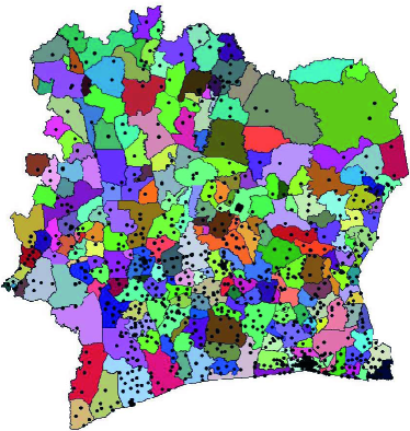
Figure 4: (a) Position of Orange’s GSM antennas in Ivory Coast [35]. The sub-prefectures are shown by different colors.

We first split the CDR dataset into two parts, where part one corresponds to the calls made in the first one-week period from the $9^{\mbox{th}}$ to $15^{\mbox{th}}$ of April, and part two corresponds to the calls made in the second one-week period from the $16^{\mbox{th}}$ to $22^{\mbox{nd}}$ of April. We then restrict our attention only to users who are active in both weeks, i.e., the users who made at least one call in each of the two weeks. There are $N=46986$ such users, and overall they connected to $K=1211$ antennas. Each user, on average, made $101.2$ calls and connected to $6.7$ different antennas. We consider the coverage region of each antenna to be a location. We disregard the timing information of the calls and construct the histograms of the calling patterns of each user in each week. Thus, the histogram $\Gamma_{x_{\bm{\sigma}(i)}}$ (respectively, $\Gamma_{y_{i}}$) of user $i$ in the first (respectively, second) week gives the relative fractions of calls made by the user in various locations in the first (respectively, second) week. The set $\psi_{1}$ (respectively, $\psi_{2}$) consists of the histograms computed over the first week (respectively, second week).

IV-A2 Matching accuracy with different metrics

After computing the histograms, we construct the complete bipartite graph $G$ shown in Figure 2 and described in Section III-B. We choose edge weights $w_{ji}$ given in (7) and compute, by using (A1), a minimum-weight maximal matching on $G$. The obtained result is shown in the first row of Table II. Of $46986$ users, $9927$ are correctly matched, which gives an accuracy of $21.1\%$. This means that, given the proportions of calls of users from different antennas during two consecutive weeks, we are able to correctly match more than one-fifth of them.

Dataset	Characteristics		Choice of metric in (A1)
	$N$	$K$	proposed	$l_{1}$	cosine	dot
CDR	$46986$	$1211$	$21.1\%$	$18.6\%$	$16.4\%$	$13.3\%$
WBH	$121$	$83219$	$90.0\%$	$81.1\%$	$72.7\%$	$64.4\%$
GL	$154$	$1024$	$58.4\%$	$51.3\%$	$52.0\%$	$46.8\%$

TABLE II: Matching accuracy obtained on $G$ in Figure 2 by using (A1) with various choices for the distance/similarity measures between the histograms defined in  (7), (6), (5), and (4). The proposed weight function consistently yields the highest accuracy for all three datasets.

We also compare the matching accuracy obtained by using the distance measure (7) with the accuracy obtained by using the distance measures given in (4) and (6), as well as the similarity measure of (5). We observe from the table that the matching accuracy obtained by using the weight function proposed in (7) is significantly higher than that obtained by using any of the other heuristic measures. We remark that the naive approach of deciding on a purely random matching between the histograms yields, on average, one correctly matched user. The resulting accuracy ($0.002\%$) is negligible compared to those obtained in Table II.

IV-A3 Effect of varying the number $N$ of users

In this experiment, we keep $U_{1}=U_{2}$ but vary $|U_{1}|$. We first choose uniformly at random a subset of the $46986$ users considered in the previous experiment. We denote the subset size by $N$. We then choose sets $\psi_{1}$ and $\psi_{2}$ to be the histograms associated with the $N$ chosen users in the first week and the second week, respectively. We then apply (A1) to the graph $G$ of Figure 2 with different choices of edge weights. For each value of $N$ we repeat the experiment several times, choosing the subset randomly and performing the matching. The obtained average accuracies are shown in Figure 5 as a function of $N$ for each choice of edge weight. We observe from Figure 5 that as the value of $N$ increases, the matching accuracy under all metrics decreases. This is expected because as $N$ increases, the habits of the users start resembling those of others, and it becomes more difficult to distinguish the histograms of one user from those of others. Hence, the matching accuracy decreases.

\psfrag{A}[Bc][Bc]{\small{Accuracy ($\%$)}}\psfrag{x}[Bc][Bc]{\small{$N$}}\psfrag{S}[Bc][Bc]{\small{$\psi_{1}$}}\psfrag{U}[Bc][Bc]{\small{$\psi_{2}$}}\psfrag{W}[Bc][Bc]{\small{$|\psi_{1}|=|\psi_{2}|=N$}}\psfrag{p}[l][l]{\footnotesize{\text{proposed}}}\psfrag{l}[l][l]{\footnotesize{\text{$l_{1}$-norm}}}\psfrag{c}[l][l]{\footnotesize{\text{cosine}}}\psfrag{d}[l][l]{\footnotesize{\text{dot}}}\includegraphics[width=433.62pt]{CDRNSim2.eps}

Figure 5: The obtained average accuracy by using different edge weights as a function of the number of users $N$, in the setting where the histograms in sets $\psi_{1}$ and $\psi_{2}$ are generated by the same set of $N$ users (i.e., $U_{1}=U_{2}$). The measures are defined in (7), (6), (4), and (5). The $90\%$ confidence interval is also shown for our proposed metric. We observe that increasing the number of users $N$ leads to a reduction in the matching accuracy.

Furthermore, although the $21.1\%$ accuracy obtained with the proposed metric of (7) in Table II might seem small at first, it is associated with a large value of $N$. If the number of users were smaller, the accuracy would be higher (e.g., $78\%$ for $1000$ users).

IV-A4 Matching different subsets of users

Following the discussion in Section III-D, here we investigate the practical scenario where the histograms in sets $\psi_{1}$ and $\psi_{2}$ belong to different sets of distinct users. In other words, in this experiment $U_{1}\neq U_{2}$. We first consider the setting in which we are given histograms of all users on the second week but only a subset of users on the first week. That is, $U_{1}\subset U_{2}$, as depicted in Figure 3(a).

We let $\psi_{2}$ be the collection of histograms of all the $N=46986$ users on the second week. For $\psi_{1}$ we use the collection of histograms of a randomly chosen subset of users on the first week. We construct $G$ in Figure 3(a) with edge weights in (7) and run (A1). The resulting matching has a size equal to $|\psi_{1}|$. The number of correctly matched histograms in the set $\psi_{1}$ divided by $|\psi_{1}|$ defines the obtained accuracy. Figure 6 shows the average number of correct matches and the average accuracy obtained for different values of $|\psi_{1}|$, where the results are averaged over several repetitions of the experiment.

\psfrag{A}[Bc][Bc]{\small{Accuracy ($\%$)}}\psfrag{B}[Bc][Bc]{\small{$\#$ corr. matches}}\psfrag{x}[Bc][Bc]{\small{Number of histograms in the first dataset ($|\psi_{1}|$)}}\psfrag{S}[Bc][Bc]{\small{$\psi_{1}$}}\psfrag{U}[Bc][Bc]{\small{$\psi_{2}$}}\psfrag{L}[l][l]{\scriptsize{Accuracy}}\psfrag{G}[l][l]{\scriptsize{$\#$ corr. matches}}\psfrag{W}[Bc][Bc]{\parbox[c]{56.9055pt}{\small{ $|\psi_{2}|=N$ \\ $|\psi_{1}|<|\psi_{2}|$}}}\includegraphics[width=433.62pt]{CDRNVar2C.eps}

Figure 6: The average number of correct matches and the average accuracy as a function of $|\psi_{1}|$ in the setting where we are given histograms of all users on the second week (i.e., $|\psi_{2}|=N$) but only a subset of users on the first week (i.e., $|\psi_{1}|<N$). The leftmost point represents one-by-one user matching approach, which yields the smallest accuracy.

The leftmost point represents one-by-one user matching approach, which yields the smallest accuracy. From a user’s perspective, as $|\psi_{1}|$ increases, the adversary has more information available and thus can obtain a better matching. Hence, the obtained matching accuracy increases. This observation has important implications in the perspective of privacy of anonymized statistics. A user’s privacy depends not only on how much her trajectory is revealed to the adversary, but also on how much of others’ trajectories are revealed to the adversary.

In the second part of this experiment, we consider the setting where $|U_{1}\cap U_{2}|=r<N$. This is the setting depicted in Figure 3(b). We choose uniformly at random a set of histograms from the first week and from the second week, such that $|U_{1}|=|U_{2}|=5000$, and $|U_{1}\cap U_{2}|=3750$. We choose these values as an example. We then construct $G$ in Figure 3(b) with edge weights given in (7). We first choose $3750$ of the unlabeled histograms in $U_{1}$ and matched them to $3750$ of the labeled histograms in $U_{2}$, such that the summation of the distance between the matched pairs is minimized. We do this by applying (A2) with $r=3750$ to $G$. Alternatively, we match all the $5000$ unlabeled histograms in $U_{1}$ to the labeled histograms in $U_{2}$ by applying (A1) to $G$. The obtained results are shown in Table III. Although the first approach yields a smaller number of correct matches ($1340$ versus $1672$) compared to the second approach, it yields a larger percentage of correct matches ($36\%$ versus $33\%$). Therefore, it makes sense to use (A2) instead of (A1) when the adversary is interested in maximizing his percentage accuracy (i.e., number of correct matches divided by the size of the outputted matching).

Algorithm	matching size	$\#$ correct matches	Percentage accuracy	$\#$ incorrect matches
(A2) with $r=3750$	3750	$1340$	$36\%$	$2410$
(A1)	5000	$1672$	$33\%$	$3328$

TABLE III: Obtained matching result for the case $|U_{1}\cap U_{2}|=r<N$ depicted in Figure 3(b) with $r=3750$ and $N=5000$. Compared to the second approach, the first approach yields a smaller number of correct matches but a larger percentage of correct matches.

IV-A5 Effect of varying the time-duration of data collection

We now investigate how the matching accuracy is affected by the time-duration over which users’ statistics are computed. We consider all users who were active on each Monday of the two-week period, i.e., users who made at least one call on Monday $9^{\text{th}}$ and on Monday $16^{\text{th}}$ of April. There are $N=30937$ such users. In the first part of this experiment, the set $\psi_{1}$ (respectively, $\psi_{2}$) corresponds to the histograms of the number of calls of this $N$ users from the $K$ locations (i.e., GSM antennas) during the first Monday (respectively, second Monday). We then construct graph $G$ illustrated in Figure 2 with different choices of edge weights, and run (A1). The obtained accuracy, marked on the x-axis by “Mon”, is shown in Figure 7.

In the second part of this experiment, we increase the time-duration over which we compute users’ statistics. We compute the statistics of the same $N$ users during the Monday and Tuesday of the first week and of the second week. Thus, the set $\psi_{1}$ (respectively, $\psi_{2}$) now corresponds to the histograms of the number of calls of the $N$ users from the $K$ locations during the first (respectively, second) Monday and Tuesday. We then construct the graph $G$ with different choices of edge weights and run (A1). The obtained matching accuracy, marked by “Mon-Tue”, is shown in Figure 7. Similarly, we increase the number of considered days for every user and repeat the experiment. These results are shown in the figure as well.

\psfrag{A}[Bc][Bc]{\small{Accuracy ($\%$)}}\psfrag{M}[Bc][Bc]{\small{Time duration included in the dataset}}\psfrag{a}[Bc][Bc]{\footnotesize{Mon}}\psfrag{b}[Bc][Bc]{\footnotesize{Mon--Tue}}\psfrag{c}[Bc][Bc]{\footnotesize{Mon--Wed}}\psfrag{d}[Bc][Bc]{\footnotesize{Mon--Thu}}\psfrag{e}[Bc][Bc]{\footnotesize{Mon--Fri}}\psfrag{f}[Bc][Bc]{\footnotesize{Mon--Sat}}\psfrag{g}[Bc][Bc]{\footnotesize{Mon--Sun}}\psfrag{S}[Bc][Bc]{\small{$\psi_{1}$}}\psfrag{U}[Bc][Bc]{\footnotesize{$\psi_{2}$}}\psfrag{W}[Bc][Bc]{\footnotesize{$|\psi_{1}|=|\psi_{2}|=N$}}\psfrag{p}[l][l]{\footnotesize{\text{proposed}}}\psfrag{l}[l][l]{\footnotesize{\text{$l_{1}$-norm}}}\psfrag{C}[l][l]{\footnotesize{\text{cosine}}}\psfrag{D}[l][l]{\footnotesize{\text{dot}}}\includegraphics[width=433.62pt]{CDRVarDay2.eps}

Figure 7: The obtained matching accuracy ($N=30937$) with different choices of edge weights as a function of time-duration over which users’ statistics are computed. The measures are defined in (7), (6), (4), and (5). As long as users’ habits remain stationary and ergodic, by increasing the time-duration over which statistics are computed, histograms belonging to each user become closer to each other, and thus the overall matching accuracy increases.

As can be seen from Figure 7, the matching accuracy increases as we include more days in the dataset. This is because as long as users’ habits remain stationary and ergodic, by increasing the time-duration over which statistics are computed, the two histograms belonging to each user become closer to each other, and thus the overall matching accuracy increases. Furthermore, the matching accuracy obtained by using the weight function proposed in (7) is significantly higher than that obtained by using any of the other heuristic measures. A standout feature in Figure 7 is the fact that the incremental improvement in going from Mon to Mon-Tue is lower than that observed in other data points in the graph. This is probably because Monday, April $9^{\text{th}}$ was White Monday, a public holiday in Ivory Coast. On the following day (i.e., Tuesday $10^{\text{th}}$ of April) the users made on average only $1.9$ calls compared to the average of $7.2$ calls per day.

IV-A6 Effect of location aggregation

In addition to the removal of user identifiers (i.e., anonymization), an additional well-known privacy-protection mechanism that is usually applied to mobility traces is spatial-resolution reduction, which is known also as location obfuscation or location aggregation [36, 37]. Here we investigate the effect of location aggregation on the matching accuracy.

The Orange call-data records dataset also includes a low-spatial resolution version [35] that contains the time of every call made by $500,000$ randomly chosen users and the sub-prefectures (i.e., administrative divisions within the provinces) of the antennas to which they were connected while making the call. The sub-prefectures, shown by different colors in Figure 4, in general contain multiple antennas, thus the dataset has a spatial resolution lower than the original dataset. We consider a two-week period and randomly choose a subset of size $N=46986$ active users out of the total $500,000$ users. The set $\psi_{1}$ (respectively, $\psi_{2}$) corresponds to the histograms of the number of calls of the $N$ users from each sub-prefectures (i.e., location) during the first week (respectively, second week). Users, in total, made calls from $K=237$ sub-prefectures. We then construct the complete bipartite graph $G$ illustrated in Figure 2 with edge weights given in (7), and run (A1). There are $2070$ correctly matched users, which gives an accuracy of $4.40\%$. The obtained accuracy is much lower than the $21.1\%$ obtained for the same number of users in the original high-resolution dataset. As antennas are aggregated into sub-prefectures, users’ histograms become less distinguishable and, as a result, the matching accuracy drops significantly.

IV-B Experiments on web browsing history (WBH) dataset

IV-B1 Dataset description and preprocessing

The Web History Repository [38] consists of anonymized detailed web browsing history of hundreds of users. Users can upload their anonymized usage data to the repository by using a Mozilla Firefox add-on. In order to protect the users’ privacy, all URLs and hosts are represented by a global unique identifier. The web browsing history (WBH) dataset contains the browsing history of $472$ users. Users participated in the data collection for different time-periods during the course of several years. For each user, the dataset contains every visited URL (with encrypted name), the favicon identifier associated with the URL, and the time of visit to the URL. The favicon, also known as a shortcut icon, is a small icon associated with a particular website. Generally, different URLs associated with the same website (e.g., domain name) have the same favicon and hence can be mapped to a single website. For example, if a user visits the URLs “news.yahoo.com” and “mail.yahoo.com”, the URLs will appear with different encrypted names in the database; however, both URLs will have the same favicon identifier (e.g., “1”). Thus, we can learn that the user has visited a particular website (i.e., “yahoo.com”) twice.

We remove from the dataset all URLs that do not have a favicon. We consider each website (e.g., “yahoo.com”) to be a location and treat the favicon identifier as the website identifier for each URL. We then identify the period of two consecutive weeks that has the maximum number of active users (i.e., users who visit at least one website during each of the two weeks). There are $N=121$ active users in this two-week period. They visited $K=83219$ different websites, $77935$ of which were visited by not more than one user. Figure 8 shows a log-log plot of the total number of visits to the websites by all the users in the two-week period. The y-axis values represent the popularity of the websites.

\psfrag{A}[Bc][Bc]{\small{Number of visits}}\psfrag{N}[Bc][Bc]{\small{Website identifier}}\includegraphics[width=433.62pt]{locpop1.eps}

Figure 8: The total number of visits (i.e., popularity) to the $K$ websites by all the users in the two-week period. The figure is plotted in a log-log scale and the websites are indexed according to their popularity.

We disregard the timing information of the visited websites and construct the histograms of the browsing patterns of each user in each week. Thus, the histogram $\Gamma_{x_{\bm{\sigma}(i)}}$ (respectively, $\Gamma_{y_{i}}$) of user $i$ in the first (respectively, second) week gives the relative fractions of the visits to various websites by that user in the first (respectively, second) week. The set $\psi_{1}$ (respectively, $\psi_{2}$) consists of the histograms computed over the first week (respectively, second week).

IV-B2 Matching accuracy with different metrics

We construct the graph $G$ shown in Figure 2 from the histograms and apply (A1) to $G$ with different choices of edge weights. The obtained results are shown in the second row of Table II. We observe that the matching accuracy obtained by using the weight function proposed in (7) is significantly higher than that obtained by using any of the other heuristic measures. Furthermore, given the proportions of visited websites during two consecutive weeks, we are able to correctly match almost all of them.

IV-B3 Considering popular websites

One reason we obtain a high matching accuracy is that some websites are visited by only a small number of users during the two-week period, hence it is easy to match those users. We investigate this effect as follows. We consider all users who visited at least one of the top $5$ popular websites, in Figure 8. There are $N=102$ such users. We consider a subset (of size not less than $5$) of the most popular of the visited websites (refer to Figure 8). We then keep for every user $i$ ($1\leq i\leq 102$) the elements of $\Gamma_{x_{\bm{\sigma}(i)}}$ and $\Gamma_{y_{i}}$ that correspond to the considered subset of websites, and we set the remaining elements equal to zero. We then re-normalize the remaining histograms such that they sum to one. We reconstruct, by using different choices of edge weights, the bipartite graph $G$ in Figure 2 and run (A1) on the graph. We repeat the experiment by varying the size of the considered subset of popular websites. The result is shown in Figure 9.

\psfrag{p}[l][l]{\footnotesize{\text{proposed}}}\psfrag{l}[l][l]{\footnotesize{\text{$l_{1}$-norm}}}\psfrag{c}[l][l]{\footnotesize{\text{cosine}}}\psfrag{d}[l][l]{\footnotesize{\text{dot}}}\psfrag{A}[Bc][Bc]{\small{Accuracy ($\%$)}}\psfrag{N}[Bc][Bc]{\small{Number of websites ($K$)}}\includegraphics[width=433.62pt]{WBHmatchres1.eps}

Figure 9: Matching accuracy for the WBH dataset with $N=102$ users by using different measures when only a subset of the popular websites are considered. The measures are defined in (7), (6), (4), and (5). The proposed weight function yields the highest percentage accuracy in the matching. The popularity of the websites is shown in Figure 8.

As expected, as fewer websites are considered, we have less information available for matching; hence the matching accuracy drops. However, by considering merely the top $60$ most popular websites, we can still correctly match more than $50\%$ of users. Moreover, as in Table II, the matching accuracy obtained by using the weight function in (7) is consistently higher than that obtained by using any of the other heuristic measures.

IV-C Experiments on GeoLife (GL) GPS dataset

IV-C1 Dataset description and preprocessing

The Geolife (GL) dataset [39] contains the GPS traces of $182$ users collected over five years. The user traces in this dataset are represented by a sequence of time-stamped points, each of which contains the information of latitude and longitude. The trajectories are widely distributed over many cities in China and even some in the USA and Europe, but the majority of the data is created in the city of Beijing. In our experiments, we focus on the trajectories collected within the $5^{\text{th}}$ ring road of Beijing, which is an area approximately $39~{}\text{km}\times 39~{}\text{km}$. We first grid this area into $100~{}\text{m}\times 100~{}\text{m}$ squares. Each square represents a location. Figure 10 shows the considered area, where all the locations with a recorded GPS position are darkened. We call a particular one-week period active for a user if she has at least one recorded GPS position during the week. Figure 10 shows the active weeks for each user during the data collection campaign. As can be seen from Figure 10, the users contributed to the dataset during different periods.

\psfrag{L}[Bc][Bc]{\small{Latitude}}\psfrag{G}[Bc][Bc]{\small{Longitude}}\includegraphics[width=199.4681pt]{geolifeMap.eps}

\psfrag{U}[Bc][Bc]{\small{User ID}}\psfrag{B}[Bc][Bc]{\footnotesize{2008}}\psfrag{D}[Bc][Bc]{\footnotesize{2010}}\psfrag{F}[Bc][Bc]{\footnotesize{2012}}\psfrag{T}[Bc][Bc]{\small{Time}}\includegraphics[width=199.4681pt]{geolifePres.eps}

Figure 10: (a) Gridding of the $5^{\text{th}}$ ring road of Beijing into squares of $100~{}\text{m}\times 100~{}\text{m}$. In area has approximate size of $39~{}\text{Km}\times 39~{}\text{Km}$. The grids in which a GPS position is recorded for a user is darkened. (b) The active weeks for each user during the data collection campaign.

We filtered out all users with number of active weeks equal to $1$ and were left with $N=154$ users. The users have on average $15.4$ active weeks of data. We split each user’s trajectories into two parts, where part one corresponds to the trajectories recorded in the first half of her active weeks, and part two corresponds to the trajectories recorded in the second half of her active weeks. We construct histograms of the locations visited by each user in each week. Thus, the histogram $\Gamma_{x_{\bm{\sigma}(i)}}$ (respectively, $\Gamma_{y_{i}}$) of user $i$ in the first (respectively, second) part gives the relative fractions of recorded GPS positions from various locations (i.e., grid squares on the map) in the first (respectively, second) part of her data. The set $\psi_{1}$ (respectively, $\psi_{2}$) corresponds to the histograms of the number of recorded GPS positions of the $N$ users from the $K$ locations in their first parts (respectively, second parts).

IV-C2 Matching accuracy with different metrics

We set the side length of grid squares equal to $1000~{}\text{m}$, and we compute the histograms and apply (A1) to the graph $G$ of Figure 2 with different choices of edge weights. The obtained matching accuracy, when the side length of grid squares is $1000~{}\text{m}$, is shown in the last row of Table II. The accuracy obtained by using the weight function proposed in (7) is significantly higher than that obtained by using any of the other heuristic measures.

IV-C3 Effect of spatial resolution

We repeat the previous experiment with varying choices for the side lengths of grid squares. The resulting matching accuracies are shown in Figure 11 as a function of the side lengths. For very large side-lengths, the spatial resolution is low, hence the users’ location traces are easily confused, thus leading to low matching accuracy. For very small side-lengths, there are too many locations in the sense that the inherent noise in the GPS trajectories come into effect, which leads to an over-fitting of the data, and thus the matching accuracy is again low. Therefore, the accuracy is maximum for moderate side-lengths – around $100~{}\text{m}$ in the figure.

\psfrag{p}[l][l]{\footnotesize{\text{proposed}}}\psfrag{l}[l][l]{\footnotesize{\text{$l_{1}$-norm}}}\psfrag{c}[l][l]{\footnotesize{\text{cosine}}}\psfrag{d}[l][l]{\footnotesize{\text{dot}}}\psfrag{A}[Bc][Bc]{\small{Accuracy ($\%$)}}\psfrag{G}[Bc][Bc]{\small{Side lengths of grid squares (in meters)}}\includegraphics[width=433.62pt]{geolifeAccObfAlU2.eps}

Figure 11: The evolution of the matching accuracy for the GL dataset ($N=154$) as a function of the grid side-length by using different metrics. The measures are defined in (7), (6), (4), and (5). The accuracy is maximum for moderate side-lengths.

IV-C4 Comparison with existing work

In [17] the authors propose a de-anonymization scheme based on a mobility model called the Mobility Markov Chain (MMC) and applied it to the GL dataset. In their approach, an MMC is constructed for each user from her mobility traces observed during the training phase and during the test phase. Distance metrics between MMCs are then used to link a user’s trace from the test phase to the corresponding trace in the training phase. There are three main differences between their approach and ours. First, in their approach, the set of locations that a user visits is learned by applying a clustering algorithm to the user’s GPS trajectories. The clustering algorithm identifies the accumulation regions of the user’s trajectory that is then used to represent the set of locations that the user visits, whereas in our approach, we partition the map area into squares that represent the set of locations. Second, they use the timing information present in the users’ trajectories to learn the MMCs, whereas in our case we disregard all the timing information present in the trajectories and only consider the fraction of visits to different locations. Third, they de-anonymize the users one-by-one, whereas we simultaneously de-anonymize all the users.

In [17], the authors report a de-anonymization accuracy of up to $45\%$ on $77$ users in the setting where the regions identified from the clustering algorithm have a maximum radius equal to $500~{}\text{m}$. In comparison, our scheme obtains a de-anonymization accuracy of up to $60\%$ for $154$ users in the setting where the side lengths of grid squares range from $300~{}\text{m}$ to $1000~{}\text{m}$. If we do one-by-one user de-anonymization, this accuracy drops down to $50\%$, however it still remains higher than the $45\%$ reported in [17]. We believe that this is because by using a complicated and dynamic model such as MMC, there is a substantial over fitting of the user data to the model. In [17], a $K\times K$ transition probability matrix is fitted to each trace, whereas in our approach a $K$-length probability vector is fitted. This leads to poorer performances because the model learned from the first dataset does not “generalize” well to the second dataset.

IV-D Running time

Here we present the timing information of performing the de-anonymization attacks that are given in Table II. We consider only the case where our proposed metric is used. The running times are given for MATLAB version $8.3.0.532$ running on a Lenovo Thinkpad T$410$ equipped with Intel i$7$ processor with clock speed of $2.67$ GHz, with $8$ Gb of RAM, and with Microsoft Windows $7$ $64$-bit operating system.

The running time for computing the edge weights ($w_{ji}$ in (7)) of graph $G$ and for running (A1) on $G$ are $41~{}\text{min}$ and $432~{}\text{min}$, respectively, for the CDR dataset. The respective numbers for the WBH dataset are $6~{}\text{sec}$ and $0.1~{}\text{sec}$ for computing the edge weights of $G$ and for running (A1) on $G$, respectively, The respective numbers for the GL dataset are $0.9~{}\text{sec}$ and $0.2~{}\text{sec}$ for computing the edge weights of $G$ and for running (A1) on $G$, respectively. Note that the reported numbers do not include the preprocessing time, that is, the time required for computing the histograms from the raw data.

V Privacy enhancing mechanisms

We demonstrated by our experiments in Section IV that applying anonymization to histograms of users’ behavior is not effective in protecting the users’ identities from an adversary who has access to auxiliary knowledge about the users. In this section, we discuss additional privacy-preserving mechanisms that can be applied to the histograms in order to make it difficult for the adversary to identify the users. These mechanisms essentially make the released histograms closer to each other so that there is greater scope for confusion in distinguishing them from each other, and thus the matching accuracy declines.

V-A Basic data coarsening and data suppression

Two popular categories of privacy-preserving mechanisms are data obfuscation and data suppression methods [40]. An example of data coarsening is spatial resolution reduction, which can be achieved by aggregating different locations into one. We investigated the latter in our experiments in Section IV-A6 and in Figure 11. Data suppression is the process of restricting the released data associated with each user. For example, in our experiment in Figure 9 for the WBH dataset, we consider only the subset of popular websites (i.e., websites that are visited by most users) and publish the histograms values associated with this subset. Another example is time-domain restriction, which refers to the process of limiting the time-period over which the histograms are computed. We investigated this approach in our experiment in Figure 7 for the CDR dataset. Another popular privacy-preserving mechanism is $k$-anonymization, which we investigate in the next subsection.

V-B $k$-Anonymization via micro-aggregation

A released dataset is said to have the $k$-anonymity property if the data for each user contained in the dataset is identical to the data for at least $k-1$ other users [41]. One mechanism for guaranteeing $k$-anonymity for a dataset is by means of micro-aggregation [42]. In micro-aggregation, users’ data are partitioned into different clusters such that each cluster contains data of at least $k$ users. The average of the data within each cluster is computed and then used to replace the original data values of all the users within the cluster. These new data values are then released, resulting in a dataset with the $k$-anonymity property. In micro-aggregation, the partitioning is done by using a criterion of minimum within-cluster information loss, and it has been shown that finding the optimal partitioning is NP-hard [43]. In the following, we define micro-aggregation in mathematical terms, and describe how our matching method can be adapted to de-anonymize micro-aggregated histograms of users’ data.

V-B1 Micro-aggregation

Let $\left\{C_{1},C_{2},\ldots,C_{g}\right\}$ be a partitioning of the users $U_{1}$ (i.e., the users who generate the histograms $\psi_{1}$) into $g$ clusters. That is, $U_{1}=\cup_{q=1}^{g}C_{q}$ and $C_{q}\cap C_{q^{\prime}}=\emptyset$ for $q\neq q^{\prime}$. We later elaborate on the criteria for choosing the set $\left\{C_{q}\right\}_{1\leq q\leq g}$. Furthermore, define $k=\min_{1\leq q\leq g}|C_{q}|$, and

$$\Gamma_{C_{q}}=\frac{1}{|C_{q}|}\sum_{j\in C_{q}}\Gamma_{x_{j}},$$ (10)

for $1\leq q\leq g$, which represent the average of histograms of all users within each cluster. In micro-aggregation, instead of releasing the set of histograms $\psi_{1}$, the set of micro-aggregated histograms $\widetilde{\psi}_{1}=\left\{\widetilde{\Gamma}_{x_{j}}\right\}$ is released, where $\widetilde{\Gamma}_{x_{j}}=\Gamma_{C_{q}}$ for $j\in C_{q}$ and for $1\leq q\leq g$. It is straightforward to see that when $\widetilde{\psi}_{1}$ is released, every user in set $U_{1}$ is guaranteed $k$-anonymity.

Although micro-aggregation guarantees $k$-anonymity to the users, it distorts the released dataset. Specifically, every histogram $\Gamma_{x_{j}}$ is replaced by $\widetilde{\Gamma}_{x_{j}}$. The criteria for obtaining $\left\{C_{q}\right\}_{1\leq q\leq g}$ in micro-aggregation is to minimize the total distortion to the data, for a given value of $k$. In the literature, the $l_{2}$-norm is often used to measure the distortion [44], however because the histograms lie on the probability simplex, we use the $l_{1}$-norm to measure the distortion. In particular the total added distortion, which is also called information loss, is $\sum_{q=1}^{g}\sum_{j\in C_{q}}\left\|\Gamma_{x_{j}}-\Gamma_{C_{q}}\right\|_{1}.$ The maximum information loss occurs when all the users are partitioned into a single cluster, i.e., when $g=1$. The information loss in this case is $\sum_{j=1}^{N}\left\|\Gamma_{x_{j}}-\overline{\Gamma}_{x}\right\|_{1}$, where $\overline{\Gamma}_{x}=\sum_{j=1}^{N}\Gamma_{x_{j}}/N$. Consequently, we can define a normalized information loss measure as follows:

$$L=\sum_{q=1}^{g}\sum_{j\in C_{q}}\left\|\Gamma_{x_{j}}-\Gamma_{C_{q}}\right\|_{1}\left/\sum_{j=1}^{N}\left\|\Gamma_{x_{j}}-\overline{\Gamma}_{x}\right\|_{1}\right..$$ (11)

The extreme case, $L=0$, represents the scenario where no micro-aggregation is performed (i.e., $g=N$) and where all users are guaranteed $1$-anonymity. The other extreme case, $L=1$, represents the scenario where $g=1$ and where all users are guaranteed $N$-anonymity. For a given value of $k$, we seek the partitioning $\left\{C_{q}\right\}_{1\leq q\leq g}$ whose normalized information loss $L$ given in (11) is as small as possible. In our following experiment, we use the algorithm proposed in [44] for performing micro-aggregation, where we adapt the algorithm to measure the distortion by using $l_{1}$-norm.

V-B2 Experimental evaluations

Here we evaluate the effectiveness of the matching algorithm when micro-aggregation is performed on the unlabeled histograms $\psi_{1}$. We consider an adversary who has access to the labeled histograms $\psi_{2}$ and is interested in matching these histograms to the micro-aggregated ones in $\widetilde{\psi}_{1}$. We consider two different notions of accuracy for the matching. Let the labeled histogram $\Gamma_{y_{i}}$ be matched to the unlabeled micro-aggregated histogram $\widetilde{\Gamma}_{x_{j}}$. According to our first notion, there is a correct match if $j=\bm{\sigma}(i)$, where $\bm{\sigma}$ is defined in (2). According to our second notion, there is a correct match if $\widetilde{\Gamma}_{x_{j}}=\widetilde{\Gamma}_{x_{\bm{\sigma}(i)}}$. The former notion of accuracy (called user-level) measures the number of correctly matched users and is the same notion that we used in our experiments in Section IV, whereas the latter notion (called cluster-level) measures the number of users whose $k$-anonymity class (i.e., cluster) is correctly identified.

For the CDR dataset, we consider the setting described in Section IV-A3. In particular, we randomly choose $N=1000$ out of the 46986 users and construct the sets $\psi_{1}$ and $\psi_{2}$. For the WBH dataset, we consider the subset of the top $K=100$ popular websites and construct the sets of histograms $\psi_{1}$ and $\psi_{2}$ as described in Section IV-B3. For the GL dataset, we consider the setting described in Section IV-C2 when grid side-length is set equal to $1000~{}\text{m}$.

For each dataset, we perform micro-aggregation with different values of $k$ on the set $\psi_{1}$. We then perform the matching between $\widetilde{\psi}_{1}$ and $\psi_{2}$ by using only the proposed metric of (7). The obtained accuracies are shown in Figure 12(a) and 12(b) and 12(c) for the CDR, WBH, and GL dataset, respectively. The figures also show the normalized information loss $L$ defined in (11) and the normalized number of clusters (i.e, $g/N$), expressed in percentages.

\psfrag{u}[l][Bc]{\scriptsize{U-Lev. accuracy}}\psfrag{c}[l][Bc]{\scriptsize{C-Lev. accuracy}}\psfrag{i}[l][Bc]{\scriptsize{Information loss}}\psfrag{n}[l][Bc]{\scriptsize{$\#$ clusters}}\psfrag{k}[Bc][Bc]{\small{$k$}}\psfrag{p}[Bc][Bc]{\small{$\%$}}\includegraphics[width=260.17464pt]{microAggCDR.eps}

(a) CDR dataset ($N=1000$)

\psfrag{k}[Bc][Bc]{\small{$k$}}\psfrag{p}[Bc][Bc]{\small{$\%$}}\includegraphics[width=199.4681pt]{microAggWBH2.eps}

(b) WBH dataset ($N=102$)

\psfrag{k}[Bc][Bc]{\small{$k$}}\psfrag{p}[Bc][Bc]{\small{$\%$}}\includegraphics[width=199.4681pt]{microAgggeo.eps}

(c) GL dataset ($N=154$)

Figure 12: The trade-off between user-level (denoted by U-Lev.) and cluster-level (denoted by C-Lev.) matching accuracies and the information loss $L$ as $k$-anonymity is guaranteed to the users. As $k$ increases, more distortion is added to the histograms (i.e., more information is lost) but the user-level accuracy drops meaning that the users enjoy higher privacy with respect to the adversary. The cluster-level accuracy however experiences much less fluctuation.

In the extreme case with $k=1$, no micro-aggregation is performed; therefore, $g=N$, $L=0$, and the user-level accuracy is equal to the cluster-level accuracy. In the other extreme case, $k=N$, and all the released unlabeled histograms are identical; therefore, the information loss is maximum ($L=1$), and while the user-level accuracy is minimum, the cluster-level accuracy is maximum. As $k$ increases to about $10$, the user-level accuracy dramatically drops, hence the users enjoy an increased level of privacy guarantee, whereas the cluster-level accuracy remains almost the same for all values of $k$.

VI Conclusion

We have studied the task of identifying users from the statistics of their behavioral patterns. Specifically, given an anonymized dataset in the form of histograms belonging to a set of users and another independent set of histograms generated by the same set of users, we have shown that it is possible to identify the identities of the users in the first dataset to a surprising level of accuracy by matching the statistical characteristics of the users’ behaviors across the two datasets. Thus data histograms act as fingerprints for identifying users. Our proposed solution can be implemented via a minimum-weight maximal matching algorithm on a complete weighted bipartite graph and yields higher accuracy than heuristics-based methods on three different datasets of different nature. We have studied the performance of the algorithm over a wide range of experimental conditions and demonstrated the effect of various factors, such as the number of users, the resolution of the data, the duration of the data collection, and the amount of data suppressed, on the accuracy of the matching algorithm. We have gained the insight that the simultaneous matching of the users yields higher accuracy compared to one-by-one user matching. Furthermore, we have demonstrated the power of simplicity of statistics: Identification based only on data statistics can sometimes result in higher accuracy than existing methods based on more complicated data models. We have further studied the performance of the algorithm under privacy-enhancement techniques, such as $k$-anonymization, and demonstrated the effect of $k$ on the matching accuracy. Our results suggest that users can be identified, to a surprisingly high level of accuracy, even from the statistics of their behavior. Moreover, using the correct metric and optimal matching algorithm can lead to a significant improvement in matching accuracy over heuristics-based methods. Privacy enhancement via $k$-anonymization and data obfuscation can reduce identification accuracy, but the accuracy remains non-negligible for moderate levels of data distortion.

VII Acknowledgments

We thank Jacques Raguenez and Vincent Blondel for granting us access to the Orange CDR dataset. We thank Alessandra Sala for her feedback on the manuscript.

References

- [1] J. Unnikrishnan and F. Movahedi Naini, “De-anonymizing private data by matching statistics,” in 51th Annual Allerton Conference, 2013.
- [2] J. Unnikrishnan, “Asymptotically optimal matching of multiple sequences to source distributions and training sequences,” IEEE Trans. Inf. Theory, vol. 61, 2015.
- [3] P. Resnick and H. R. Varian, “Recommender systems,” Communications of the ACM, vol. 40, no. 3, pp. 56–58, 1997.
- [4] A. Narayanan and V. Shmatikov, “Robust de-anonymization of large sparse datasets,” in Proceedings of IEEE Symposium on Security and Privacy, 2008.
- [5] A. K. Elmagarmid, P. G. Ipeirotis, and V. S. Verykios, “Duplicate record detection: A survey,” IEEE Trans. Knowl. Data Eng., 2007.
- [6] D. V. Kalashnikov, Z. Chen, S. Mehrotra, and R. Nuray-Turan, “Web people search via connection analysis,” IEEE Trans. Knowl. Data Eng., 2008.
- [7] E. Bengtson and D. Roth, “Understanding the value of features for coreference resolution,” in EMNLP Conference, 2008.
- [8] A. Stolerman, R. Overdorf, S. Afroz, and R. Greenstadt, “Breaking the closed-world assumption in stylometric authorship attribution,” in Advances in Digital Forensics X. Springer, 2014.
- [9] S. Afroz, A. C. Islam, A. Stolerman, R. Greenstadt, and D. McCoy, “Doppelgänger finder: Taking stylometry to the underground,” in Security and Privacy (SP), 2014 IEEE Symposium on. IEEE, 2014.
- [10] O. Peled, M. Fire, L. Rokach, and Y. Elovici, “Entity matching in online social networks,” in IEEE SocialCom, 2013.
- [11] J. Liu, F. Zhang, X. Song, Y.-I. Song, C.-Y. Lin, and H.-W. Hon, “What’s in a name?: an unsupervised approach to link users across communities,” in ACM WSDM, 2013.
- [12] L. Sweeney, “Weaving technology and policy together to maintain confidentiality,” The Journal of Law, Medicine & Ethics, 1997.
- [13] H. Zang and J. Bolot, “Anonymization of location data does not work: A large-scale measurement study,” in ACM MobiCom, 2011.
- [14] X. Xiao, Y. Zheng, Q. Luo, and X. Xie, “Finding similar users using category-based location history,” in ACM SIGSPATIAL, 2010.
- [15] C. Y. Ma, D. K. Yau, N. K. Yip, and N. S. Rao, “Privacy vulnerability of published anonymous mobility traces,” in MobiCom, 2010.
- [16] J. Freudiger, R. Shokri, and J.-P. Hubaux, “Evaluating the privacy risk of location-based services,” in Financial Cryptography and Data Security. Springer, 2012.
- [17] S. Gambs, M.-O. Killijian, and M. Núñez del Prado Cortez, “De-anonymization attack on geolocated data,” Journal of Computer and System Sciences, 2014.
- [18] Y. De Mulder, G. Danezis, L. Batina, and B. Preneel, “Identification via location-profiling in gsm networks,” in ACM WPES, 2008.
- [19] A. Machanavajjhala, D. Kifer, J. Abowd, J. Gehrke, and L. Vilhuber, “Privacy: Theory meets practice on the map,” in IEEE ICDE, 2008.
- [20] L. Olejnik, C. Castelluccia, and A. Janc, “On the uniqueness of web browsing history patterns,” annals of telecommunications-annales des télécommunications, vol. 69, no. 1-2, pp. 63–74, 2014.
- [21] T.-F. Yen, Y. Xie, F. Yu, R. P. Yu, and M. Abadi, “Host fingerprinting and tracking on the web: Privacy and security implications.” in NDSS, 2012.
- [22] K. Sharad and G. Danezis, “De-anonymizing d4d datasets,” in HotPETs, 2013.
- [23] M. Srivatsa and M. Hicks, “Deanonymizing mobility traces: Using social network as a side-channel,” in ACM CCS, 2012.
- [24] Y.-A. de Montjoye, C. A. Hidalgo, M. Verleysen, and V. D. Blondel, “Unique in the Crowd: The privacy bounds of human mobility,” Scientific Reports, 2013.
- [25] R. Shokri, G. Theodorakopoulos, J.-Y. Le Boudec, and J.-P. Hubaux, “Quantifying location privacy,” in Security and Privacy (SP), 2011 IEEE Symposium on. IEEE, 2011, pp. 247–262.
- [26] G. Danezis and C. Troncoso, “Vida: How to use bayesian inference to de-anonymize persistent communications,” in Privacy Enhancing Technologies. Springer, 2009, pp. 56–72.
- [27] C. Troncoso, B. Gierlichs, B. Preneel, and I. Verbauwhede, “Perfect matching disclosure attacks,” in Privacy Enhancing Technologies. Springer, 2008, pp. 2–23.
- [28] P. Pedarsani and M. Grossglauser, “On the privacy of anonymized networks,” in ACM KDD, 2011.
- [29] T. Hastie, R. Tibshirani, and J. Friedman, The elements of statistical learning. Springer, 2009, vol. 2, no. 1.
- [30] T. M. Cover and J. A. Thomas, Elements of Information Theory 2nd Edition. Wiley-Interscience, 2006.
- [31] L. Ramshaw and R. E. Tarjan, “A weight-scaling algorithm for min-cost imperfect matchings in bipartite graphs,” in IEEE FOCS, 2012.
- [32] M. L. Fredman and R. E. Tarjan, “Fibonacci heaps and their uses in improved network optimization algorithms,” JACM, 1987.
- [33] W. Cook, W. Cunningham, W. Pulleyblank, and A. Schrijver, Combinatorial Optimization, ser. Wiley Series in Discrete Mathematics and Optimization. Wiley, 2011.
- [34] R. Duan and S. Pettie, “Linear-time approximation for maximum weight matching,” J. ACM, vol. 61, no. 1, pp. 1:1–1:23, Jan. 2014.
- [35] V. D. Blondel, M. Esch, C. Chan, F. Clerot, P. Deville, E. Huens, F. Morlot, Z. Smoreda, and C. Ziemlicki, “Data for development: the d4d challenge on mobile phone data,” arXiv preprint arXiv:1210.0137, 2012.
- [36] K. L. Huang, S. S. Kanhere, and W. Hu, “Preserving privacy in participatory sensing systems,” Computer Communications, 2010.
- [37] D. Christin, A. Reinhardt, S. S. Kanhere, and M. Hollick, “A survey on privacy in mobile participatory sensing applications,” Journal of Systems and Software, 2011.
- [38] E. Herder, R. Kawase, and G. Papadakis, “Experiences in building the public web history repository,” in Proc. of Datatel Workshop, 2011.
- [39] Y. Zheng, Q. Li, Y. Chen, X. Xie, and W.-Y. Ma, “Understanding mobility based on gps data,” in ACM Ubicomp, 2008.
- [40] C. C. Aggarwal and S. Y. Philip, A general survey of privacy-preserving data mining models and algorithms. Springer, 2008.
- [41] L. Sweeney, “k-anonymity: A model for protecting privacy,” INT J UNCERTAIN FUZZ, 2002.
- [42] J. Domingo-Ferrer and J. M. Mateo-Sanz, “Practical data-oriented microaggregation for statistical disclosure control,” IEEE Trans. Knowl. Data Eng., 2002.
- [43] J. Domingo-Ferrer, F. Sebé, and A. Solanas, “A polynomial-time approximation to optimal multivariate microaggregation,” Computers & Mathematics with Applications, 2008.
- [44] C. Panagiotakis and G. Tziritas, “Successive group selection for microaggregation,” IEEE Trans. Knowl. Data Eng., 2013.