Stability and Minimax Optimality of Tangential Delaunay Complexes for Manifold Reconstruction

Abstract

We consider the problem of optimality in manifold reconstruction. A random sample $\mathbb{X}_{n}=\left\{X_{1},\ldots,X_{n}\right\}\subset\mathbb{R}^{D}$ composed of points close to a $d$-dimensional submanifold $M$, with or without outliers drawn in the ambient space, is observed. Based on the Tangential Delaunay Complex [4], we construct an estimator $\hat{M}$ that is ambient isotopic and Hausdorff-close to $M$ with high probability. The estimator $\hat{M}$ is built from existing algorithms. In a model with additive noise of small amplitude, we show that this estimator is asymptotically minimax optimal for the Hausdorff distance over a class of submanifolds satisfying a reach constraint. Therefore, even with no a priori information on the tangent spaces of $M$, our estimator based on Tangential Delaunay Complexes is optimal. This shows that the optimal rate of convergence can be achieved through existing algorithms. A similar result is also derived in a model with outliers. A geometric interpolation result is derived, showing that the Tangential Delaunay Complex is stable with respect to noise and perturbations of the tangent spaces. In the process, a decluttering procedure and a tangent space estimator both based on local principal component analysis (PCA) are studied.

1 Introduction

Throughout many fields of applied science, data in $\mathbb{R}^{D}$ can naturally be modeled as lying on a $d$-dimensional submanifold $M$. As $M$ may carry a lot of information about the studied phenomenon, it is then natural to consider the problem of either approximating $M$ geometrically, recovering it topologically, or both from a point sample $\mathbb{X}_{n}=\left\{X_{1},\ldots,X_{n}\right\}$. It is of particular interest in high codimension ($d\ll D$) where it can be used as a preliminary processing of the data for reducing its dimension, and then avoiding the curse of dimensionality. This problem is usually referred to as manifold reconstruction in the computational geometry community, and rather called set/support estimation or manifold learning in the statistics literature.

The computational geometry community has now been active on manifold reconstruction for many years, mainly in deterministic frameworks. In dimension $3$, [17] provides a survey of the state of the art. In higher dimension, the employed methods rely on variants of the ambient Delaunay triangulation [12, 4]. The geometric and topological guarantees are derived under the assumption that the point cloud — fixed and nonrandom — densely samples $M$ at scale $\varepsilon$, with $\varepsilon$ small enough or going to $0$.

In the statistics literature, most of the attention has been paid to approximation guarantees, rather than topological ones. The approximation bounds are given in terms of the sample size $n$, that is assumed to be large enough or going to infinity. To derive these bounds, a broad variety of assumptions on $M$ have been considered. For instance, if $M$ is a bounded convex set and $\mathbb{X}_{n}$ does not contain outliers, a natural idea is to consider the convex hull $\hat{M}=Conv(\mathbb{X}_{n})$ to be the estimator. $Conv(\mathbb{X}_{n})$ provides optimal rates of approximation for several loss functions [29, 20]. These rates depend crudely on the regularity of the boundary of the convex set $M$. In addition, $Conv(\mathbb{X}_{n})$ clearly is ambient isotopic to $M$ so that it has both good geometric and topological properties. Generalisations of the notion of convexity based on rolling ball-type assumptions such as $r$-convexity and reach bounds [14, 24] yield rich classes of sets with good geometric properties. In particular, the reach, as introduced by Federer [22], appears to be a key regularity and scale parameter [10, 24, 28].

This paper mainly follows up the two articles [4, 24], both dealing with the case of a $d$-dimensional submanifold $M\subset\mathbb{R}^{D}$ with a reach regularity condition and where the dimension $d$ is known.

On one hand, [4] focuses on a deterministic analysis and proposes a provably faithful reconstruction. The authors introduce a weighted Delaunay triangulation restricted to tangent spaces, the so-called Tangential Delaunay Complex. This paper gives a reconstruction up to ambient isotopy with approximation bounds for the Hausdorff distance along with computational complexity bounds. This work provides a simplicial complex based on the input point cloud and tangent spaces. However, it lacks stability up to now, in the sense that the assumptions used in the proofs of [4] do not resist ambient perturbations. Indeed, it heavily relies on the knowledge of the tangent spaces at each point and on the absence of noise.

On the other hand, [24] takes a statistical approach in a model possibly corrupted by additive noise, or containing outlier points. The authors derive an estimator that is proved to be minimax optimal for the Hausdorff distance ${d}_{H}$. Roughly speaking, minimax optimality of the proposed estimator means that it performs best in the worst possible case up to numerical constants, when the sample size $n$ is large enough. Although theoretically optimal, the proposed estimator appears to be intractable in practice. At last, [28] proposes a manifold estimator based on local linear patches that is tractable but fails to achieve the optimal rates.

Contribution

Our main contributions (Theorems 7, 8 and 9) make a two-way link between the approaches of [4] and [24].

From a geometric perspective, Theorem 7 shows that the Tangential Delaunay Complex of [4] can be combined with local PCA to provide a manifold estimator that is optimal in the sense of [24]. This remains possible even if data is corrupted with additive noise of small amplitude. Also, Theorems 8 and 9 show that, if outlier points are present (clutter noise), the Tangential Delaunay Complex of [4] still yields the optimal rates of [24], at the price of an additional decluttering procedure.

From a statistical point of view, our results show that the optimal rates described in [24] can be achieved by a tractable estimator $\hat{M}$ that (1) is a simplicial complex of which vertices are the data points, and (2) such that $\hat{M}$ is ambient isotopic to $M$ with high probability.

In the process, a stability result for the Tangential Delaunay Complex (Theorem 14) is proved. Let us point out that this stability is derived using an interpolation result (Theorem 11) which is interesting in its own right. Theorem 11 states that if a point cloud $\mathcal{P}$ lies close to a submanifold $M$, and that estimated tangent spaces at each sample point are given, then there is a submanifold $M^{\prime}$ (ambient isotopic, and close to $M$ for the Hausdorff distance) that interpolates $\mathcal{P}$, with $T_{p}M^{\prime}$ agreeing with the estimated tangent spaces at each point $p\in\mathcal{P}$. Moreover, the construction can be done so that the reach of $M^{\prime}$ is bounded in terms of the reach of $M$, provided that $\mathcal{P}$ is sparse, points of $\mathcal{P}$ lie close to $M$, and error on the estimated tangent spaces is small. Hence, Theorem 11 essentially allows to consider a noisy sample with estimated tangent spaces as an exact sample with exact tangent spaces on a proxy submanifold. This approach can provide stability for any algorithm that takes point cloud and tangent spaces as input, such as the so-called cocone complex [12].

Outline

This paper deals with the case where a sample $\mathbb{X}_{n}=\left\{X_{1},\ldots,X_{n}\right\}\subset\mathbb{R}^{D}$ of size $n$ is randomly drawn on/around $M$. First, the statistical framework is described (Section 2.1) together with minimax optimality (Section 2.2). Then, the main results are stated (Section 2.3).

Two models are studied, one where $\mathbb{X}_{n}$ is corrupted with additive noise, and one where $\mathbb{X}_{n}$ contains outliers. We build a simplicial complex $\hat{M}_{\mathtt{TDC}}(\mathbb{X}_{n})$ ambient isotopic to $M$ and we derive the rate of approximation for the Hausdorff distance ${d}_{H}(M,\hat{M}_{\mathtt{TDC}})$, with bounds holding uniformly over a class of submanifolds satisfying a reach regularity condition. The derived rate of convergence is minimax optimal if the amplitude $\sigma$ of the additive noise is small. With outliers, similar estimators $\hat{M}_{\mathtt{TDC\delta}}$ and $\hat{M}_{\mathtt{TDC+}}$ are built. $\hat{M}_{\mathtt{TDC}}$, $\hat{M}_{\mathtt{TDC\delta}}$ and $\hat{M}_{\mathtt{TDC+}}$ are based on the Tangential Delaunay Complex (Section 3), that is first proved to be stable (Section 4) via an interpolation result. A method to estimate tangent spaces and to remove outliers based on local Principal Component Analysis (PCA) is proposed (Section 5). We conclude with general remarks and possible extensions (Section 6). For ease of exposition, all the proofs are placed in the appendix.

Notation

In what follows, we consider a compact $d$-dimensional submanifold without boundary $M\subset\mathbb{R}^{D}$ to be reconstructed. For all $p\in M$, $T_{p}M$ designates the tangent space of $M$ at $p$. Tangent spaces will either be considered vectorial or affine depending on the context. The standard inner product in $\mathbb{R}^{D}$ is denoted by $\langle\cdot,\cdot\rangle$ and the Euclidean distance $\left\|\cdot\right\|$. We let $\mathcal{B}(p,r)$ denote the closed Euclidean ball of radius $r>0$ centered at $p$. We let $\wedge$ and $\vee$ denote respectively the minimum and the maximum of real numbers. As introduced in [22], the reach of $M$, denoted by $\mathrm{reach}(M)$ is the maximal offset radius for which the projection $\pi_{M}$ onto $M$ is well defined. Denoting by ${d}(\cdot,M)$ the distance to $M$, the medial axis of $M$ $\mathrm{med}(M)=\{x\in\mathbb{R}^{D}|\exists a\neq b\in M,\left\|x-a\right\|=\left\|x-b\right\|={d}(x,M)\}$ is the set of points which have at least two nearest neighbors on $M$. Then, $\mathrm{reach}(M)=\underset{p\in M}{\inf}{d}(p,\mathrm{med}(M))$. We simply write $\pi$ for $\pi_{M}$ when there is no possibility of confusion. For any smooth function $\Phi:\mathbb{R}^{D}\rightarrow\mathbb{R}^{D}$, we let ${d}_{a}\Phi$ and ${d}_{a}^{2}\Phi$ denote the first and second order differentials of $\Phi$ at $a\in\mathbb{R}^{D}$. For a linear map $A$, $A^{t}$ designates its transpose. Let $\left\|A\right\|_{\mathrm{op}}={\sup_{x}}\frac{\left\|Ax\right\|}{\left\|x\right\|}$ and $\left\|A\right\|_{\mathcal{F}}=\sqrt{\mathrm{trace}\left(A^{t}A\right)}$ denote respectively the operator norm induced by the Euclidean norm and the Frobenius norm. The distance between two linear subspaces $U,V\subset\mathbb{R}^{D}$ of the same dimension is measured by the sine $\angle(U,V)=\underset{u\in U}{\max}~{}\underset{v^{\prime}\in V^{\perp}}{\max}\dfrac{\langle u,v^{\prime}\rangle}{\left\|u\right\|\left\|v^{\prime}\right\|}=\left\|\pi_{U}-\pi_{V}\right\|_{\mathrm{op}}$ of their largest principal angle. The Hausdorff distance between two compact subsets $K,K^{\prime}$ of $\mathbb{R}^{D}$ is denoted by ${d}_{H}(K,K^{\prime})=\sup_{x\in\mathbb{R}^{D}}\left|d(x,K)-d(x,K^{\prime})\right|$. Finally, we let $\cong$ denote the ambient isotopy relation in $\mathbb{R}^{D}$.

Throughout this paper, $C_{\alpha}$ will denote a generic constant depending on the parameter $\alpha$. For clarity’s sake, $c_{\alpha}$ and $K_{\alpha}$ may also be used when several constants are involved.

2 Minimax Risk and Main Results

2.1 Statistical Model

Let us describe the general statistical setting we will use to define optimality for manifold reconstruction. A statistical model $\mathcal{D}$ is a set of probability distributions on $\mathbb{R}^{D}$. In any statistical experiment, $\mathcal{D}$ is fixed and known. We observe an independent and identically distributed sample of size $n$ (or i.i.d. $n$-sample) $\mathbb{X}_{n}=\left\{X_{1},\ldots,X_{n}\right\}$ drawn according to some unknown distribution $P\in\mathcal{D}$. If no noise is allowed, the problem is to recover the support of $P$, that is, the smallest closed set $C\subset\mathbb{R}^{D}$ such that $P(C)=1$. Let us give two examples of such models $\mathcal{D}$ by describing those of interest in this paper.

Let $\mathcal{M}_{D,d,\rho}$ be the set of all compact $d$-dimensional connected submanifolds $M\subset\mathbb{R}^{D}$ without boundary satisfying $\mathrm{reach}(M)\geq\rho$. The reach assumption is crucial to avoid arbitrarily curved and pinched shapes [14]. From a reconstruction point of view, $\rho$ gives a minimal feature size on $M$, and then a minimal scale for geometric information. Every $M\in\mathcal{M}_{D,d,\rho}$ inherits a measure induced by the $d$-dimensional Hausdorff measure on $\mathbb{R}^{D}\supset M$. We denote this induced measure by $v_{M}$. Beyond the geometric restrictions induced by the lower bound $\rho$ on the reach, it also requires the natural measure $v_{M}$ to behave like a $d$-dimensional measure, up to uniform constants. Denote by $\mathcal{U}_{M}(f_{min},f_{max})$ the set of probability distributions $Q$ having a density $f$ with respect to $v_{M}$ such that $0<f_{min}\leq f(x)\leq f_{max}<\infty$ for all $x\in M$. In particular, notice that such distributions $Q\in\mathcal{U}_{M}(f_{min},f_{max})$ all have support $M$. Roughly speaking, when $Q\in\mathcal{U}_{M}(f_{min},f_{max})$, points are drawn almost uniformly on $M$. This is to ensure that the sample visits all the areas of $M$ with high probability. The noise-free model $\mathcal{G}_{D,d,f_{min},f_{max},\rho}$ consists of the set of all these almost uniform measures on submanifolds of dimension $d$ having reach greater than a fixed value $\rho>0$.

Definition 1 (Noise-free model).

$\mathcal{G}_{D,d,f_{min},f_{max},\rho}=\bigcup_{M\in\mathcal{M}_{D,d,\rho}}\mathcal{U}_{M}(f_{min},f_{max})$.

Notice that we do not explicitly impose a bound on the diameter of $M$. Actually, a bound is implicitly present in the model, as stated in the next lemma, the proof of which follows from a volume argument.

Lemma 2.

There exists $C_{d}>0$ such that for all $Q\in\mathcal{G}_{D,d,f_{min},f_{max},\rho}$ with associated $M$,

$$\mathrm{diam}(M)\leq\frac{C_{d}}{\rho^{d-1}f_{min}}=:K_{d,f_{min},\rho}.$$

Observed random variables with distribution belonging to the noise-free model $\mathcal{G}_{D,d,f_{min},f_{max},\rho}$ lie exactly on the submanifold of interest $M$. A more realistic model should allow some measurement error, as illustrated by Figure 1a. We formalize this idea with the following additive noise model.

Definition 3 (Additive noise model).

For $\sigma<\rho$, we let $\mathcal{G}_{D,d,f_{min},f_{max},\rho,\sigma}$ denote the set of distributions of random variables $X=Y+Z$, where $Y$ has distribution $Q\in\mathcal{G}_{D,d,f_{min},f_{max},\rho}$, and $\left\|Z\right\|\leq\sigma$ almost surely.

Let us emphasize that we do not require $Y$ and $Z$ to be independent, nor $Z$ to be orthogonal to $T_{Y}M$, as done for the “perpendicular” noise model of [30, 24]. This model is also slightly more general than the one considered in [28]. Notice that the noise-free model can be thought of as a particular instance of the additive noise model, since $\mathcal{G}_{D,d,f_{min},f_{max},\rho}=\mathcal{G}_{D,d,f_{min},f_{max},\rho,\sigma=0}$.

Eventually, we may include distributions contaminated with outliers uniformly drawn in a ball $\mathcal{B}_{0}$ containing $M$, as illustrated in Figure 1b. Up to translation, we can always assume that $M\ni 0$. To avoid boundary effects, $\mathcal{B}_{0}$ will be taken to contain $M$ amply, so that the outlier distribution surrounds $M$ everywhere. Since $M$ has at most diameter $K_{d,f_{min},\rho}$ from Lemma 2 we arbitrarily fix $\mathcal{B}_{0}=\mathcal{B}(0,K_{0})$, where $K_{0}=K_{d,f_{min},\rho}+\rho$. Notice that the larger the radius of $\mathcal{B}_{0}$, the easier to label the outlier points since they should be very far away from each other.

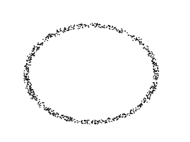
(a) Circle with noise: $d=1$, $D=2$, $\sigma>0$.

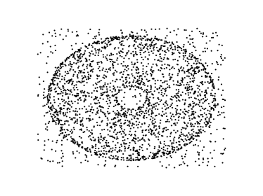
(b) Torus with outliers: $d=2$, $D=3$, $\beta<1$.

Figure 1: Point clouds $\mathbb{X}_{n}$ drawn from distributions in $\mathcal{G}_{D,d,f_{min},f_{max},\rho,\sigma}$ (left) and $\mathcal{O}_{D,d,f_{min},f_{max},\rho,\beta}$ (right).

Definition 4 (Model with outliers/Clutter noise model).

For $0<f_{min}\leq f_{max}<\infty$, $0<\beta\leq 1$, and $\rho>0$, we define $\mathcal{O}_{D,d,f_{min},f_{max},\rho,\beta}$ to be the set of mixture distributions

$$P=\beta Q+(1-\beta)U_{\mathcal{B}_{0}},$$

where $Q\in\mathcal{G}_{D,d,f_{min},f_{max},\rho}$ has support $M$ such that $0\in M$, and $U_{\mathcal{B}_{0}}$ is the uniform distribution on $\mathcal{B}_{0}=\mathcal{B}(0,K_{0})$.

Alternatively, a random variable $X$ with distribution $P\in\mathcal{O}_{D,d,f_{min},f_{max},\rho,\beta}$ can be represented as $X=VX^{\prime}+(1-V)X^{\prime\prime}$ , where $V\in\left\{0,1\right\}$ is a Bernoulli random variable with parameter $\beta$, $X^{\prime}$ has distribution in $\mathcal{G}_{D,d,f_{min},f_{max},\rho}$ and $X^{\prime\prime}$ has a uniform distribution over $\mathcal{B}_{0}$, and such that $V,X^{\prime},X^{\prime\prime}$ are independent. In particular for $\beta=1$, $\mathcal{O}_{D,d,f_{min},f_{max},\rho,\beta=1}=\mathcal{G}_{D,d,f_{min},f_{max},\rho}$.

2.2 Minimax Risk

For a probability measure $P\in\mathcal{D}$, denote by $\mathbb{E}_{P}$ — or simply $\mathbb{E}$ — the expectation with respect to the product measure $P^{(n)}$. The quantity we will be interested in is the minimax risk associated to the model $\mathcal{D}$. For $n\geq 0$,

$$R_{n}(\mathcal{D})=\inf_{\hat{M}}\sup_{P\in\mathcal{D}}\mathbb{E}_{P}\left[{d}_{{H}}\left(M,\hat{M}\right)\right],$$

where the infimum is taken over all the estimators $\hat{M}=\hat{M}\left(X_{1},\ldots,X_{n}\right)$ computed over an $n$-sample. $R_{n}(\mathcal{D})$ is the best risk that an estimator based on an $n$-sample can achieve uniformly over the class $\mathcal{D}$. It is clear from the definition that if $\mathcal{D}^{\prime}\subset\mathcal{D}$ then $R_{n}(\mathcal{D^{\prime}})\leq R_{n}(\mathcal{D})$. It follows the intuition that the broader the class of considered manifolds, the more difficult it is to estimate them uniformly well. Studying $R_{n}(\mathcal{D})$ for a fixed $n$ is a difficult task that can rarely be carried out. We will focus on the semi-asymptotic behavior of this risk. As $R_{n}(\mathcal{D})$ cannot be surpassed, its rate of convergence to $0$ as $n\rightarrow\infty$ may be seen as the best rate of approximation that an estimator can achieve. We will say that two sequences $(a_{n})_{n}$ and $(b_{n})_{n}$ are asymptotically comparable, denoted by $a_{n}\asymp b_{n}$, if there exist $c,C>0$ such that for $n$ large enough, $cb_{n}\leq a_{n}\leq Cb_{n}$.

Definition 5.

An estimator $\hat{M}$ is said to be (asymptotically) minimax optimal over $\mathcal{D}$ if

$$\sup_{P\in\mathcal{D}}\mathbb{E}_{P}\left[{d}_{{H}}\left(M,\hat{M}\right)\right]\asymp R_{n}(\mathcal{D}).$$

In other words, $\hat{M}$ is (asymptotically) minimax optimal if it achieves, up to constants, the best possible rate of convergence in the worst case.

Studying a minimax rate of convergence is twofold. On one hand, deriving an upper bound on $R_{n}$ boils down to provide an estimator and to study its quality uniformly on $\mathcal{D}$. On the other hand, bounding $R_{n}$ from below amounts to study the worst possible case in $\mathcal{D}$. This part is usually achieved with standard Bayesian techniques [27]. For the models considered in the present paper, the rates were given in [24, 26].

Theorem 6 (Theorem 3 of [26]).

We have,

$$R_{n}\left(\mathcal{G}_{D,d,f_{min},f_{max},\rho}\right)\asymp\left(\frac{\log n}{n}\right)^{2/d},$$ (Noise-free)

and for $0<\beta\leq 1$ fixed,

$$R_{n}\left(\mathcal{O}_{D,d,f_{min},f_{max},\rho,\beta}\right)\asymp\left(\frac{\log n}{\beta n}\right)^{2/d}.$$ (Clutter noise)

Since the additive noise model $\mathcal{G}_{D,d,f_{min},f_{max},\rho,\sigma}$ has not yet been considered in the literature, the behavior of the associated minimax risk is not known. Beyond this theoretical result, an interesting question is to know whether these minimax rates can be achieved by a tractable algorithm. Indeed, that proposed in [24] especially rely on a minimization problem over the class of submanifolds $\mathcal{M}_{D,d,\rho}$, which is computationally costly. In addition, the proposed estimators are themselves submanifolds, which raises storage problems. Moreover, no guarantee is given on the topology of the estimators. Throughout the present paper, we will build estimators that address these issues.

2.3 Main Results

Let us start with the additive noise model $\mathcal{G}_{D,d,f_{min},f_{max},\rho,\sigma}$, that includes in particular the noise-free case $\sigma=0$. The estimator $\hat{M}_{\mathtt{TDC}}$ is based on the Tangential Delaunay Complex (Section 3), with a tangent space estimation using a local PCA (Section 5).

Theorem 7.

$\hat{M}_{\mathtt{TDC}}=\hat{M}_{\mathtt{TDC}}(\mathbb{X}_{n})$ is a simplicial complex with vertices included in $\mathbb{X}_{n}$ such that the following holds. There exists $\lambda_{d,f_{min},f_{max}}>0$ such that if $\sigma\leq\lambda\left(\frac{\log n}{n}\right)^{1/d}$ with $\lambda\leq\lambda_{d,f_{min},f_{max}}$, then

$$\underset{n\rightarrow\infty}{\lim}\mathbb{P}\left({d}_{H}({M},\hat{M}_{\mathtt{TDC}})\leq{C_{d,f_{min},f_{max},{\rho}}}\left\{\left(\frac{\log n}{n}\right)^{2/d}\vee\lambda^{2}\right\}\text{ and }{M}\cong\hat{M}_{\mathtt{TDC}}\right)=1.$$

Moreover, for $n$ large enough,

$$\sup_{Q\in\mathcal{G}_{D,d,f_{min},f_{max},\rho,\sigma}}\mathbb{E}_{Q}{d}_{H}({M},\hat{M}_{\mathtt{TDC}})\leq{C^{\prime}_{d,f_{min},f_{max},{\rho}}}\left\{\left(\frac{\log n}{n}\right)^{2/d}\vee\lambda^{2}\right\}.$$

It is interesting to note that the constants appearing in Theorem 7 do not depend on the ambient dimension $D$. Since $R_{n}\left(\mathcal{G}_{D,d,f_{min},f_{max},\rho,\sigma}\right)\geq R_{n}\left(\mathcal{G}_{D,d,f_{min},f_{max},\rho}\right)$, we obtain immediately from Theorem 7 that $\hat{M}_{\mathtt{TDC}}$ achieves the minimax optimal rate $\left({\log n}/{n}\right)^{2/d}$ over $\mathcal{G}_{D,d,f_{min},f_{max},\rho,\sigma}$ when $\sigma\leq c_{d,f_{min},f_{max}}\left({\log n}/{n}\right)^{2/d}$. Note that the estimator of [28] achieves the rate $\left({\log n}/{n}\right)^{2/(d+2)}$ when $\sigma\leq c_{d,f_{min},f_{max}}\left({\log n}/{n}\right)^{2/(d+2)}$, so does the estimator of [25] for $\sigma<\rho$ if the noise is centered and perpendicular to the submanifold. As a consequence, $\hat{M}_{\mathtt{TDC}}$ outperforms these two existing procedures whenever $\sigma\ll\left(\log n/n\right)^{2/(d+2)}$, with the additional feature of exact topology recovery. Still, for $\sigma\gg\left(\log n/n\right)^{1/d}$, $\hat{M}_{\mathtt{TDC}}$ may perform poorly compared to [25]. This might be due to the fact that the vertices of $\hat{M}_{\mathtt{TDC}}$ are sample points themselves, while for higher noise levels, a pre-process of the data based on local averaging could be more relevant.

In the model with outliers $\mathcal{O}_{D,d,f_{min},f_{max},\rho,\beta}$, with the same procedure used to derive Theorem 7 and an additional iterative preprocessing of the data based on local PCA to remove outliers (Section 5), we design an estimator of $M$ that achieves a rate as close as wanted to the noise-free rate. Namely, for any positive $\delta<1/(d(d+1))$, we build $\hat{M}_{\mathtt{TDC\delta}}$ that satisfies the following similar statement.

Theorem 8.

$\hat{M}_{\mathtt{TDC}\delta}=\hat{M}_{\mathtt{TDC}\delta}(\mathbb{X}_{n})$ is a simplicial complex with vertices included in $\mathbb{X}_{n}$ such that

$$\underset{n\rightarrow\infty}{\lim}\mathbb{P}\left({d}_{H}({M},\hat{M}_{\mathtt{TDC\delta}})\leq C_{d,f_{min},f_{max},\rho}\left(\dfrac{\log n}{\beta n}\right)^{2/d-2\delta}\text{ and }{M}\cong\hat{M}_{\mathtt{TDC\delta}}\right)=1.$$

Moreover, for $n$ large enough,

$$\sup_{P\in\mathcal{O}_{D,d,f_{min},f_{max},\rho,\beta}}\mathbb{E}_{P}{d}_{H}({M},\hat{M}_{\mathtt{TDC\delta}})\leq C^{\prime}_{d,f_{min},f_{max},\rho}\left(\dfrac{\log n}{\beta n}\right)^{2/d-2\delta}.$$

$\hat{M}_{\mathtt{TDC\delta}}$ converges at the rate at least $\left({\log n}/{n}\right)^{2/d-2\delta}$, which is not the minimax optimal rate according to Theorem 6, but that can be set as close as desired to it. To our knowledge, $\hat{M}_{\mathtt{TDC\delta}}$ is the first explicit estimator to provably achieve such a rate in the presence of outliers. Again, it is worth noting that the constants involved in Theorem 8 do not depend on the ambient dimension $D$. The construction and computation of $\hat{M}_{\mathtt{TDC\delta}}$ is the same as $\hat{M}_{\mathtt{TDC}}$, with an extra pre-processing of the point cloud allowing to remove outliers. This decluttering procedure leads to compute, at each sample point, at most $\log(1/\delta)$ local PCA’s, instead of a single one for $\hat{M}_{\mathtt{TDC}}$.

From a theoretical point of view, there exists a (random) number of iterations of this decluttering process, from which an estimator $\hat{M}_{\mathtt{TDC+}}$ can be built to satisfy the following.

Theorem 9.

$\hat{M}_{\mathtt{TDC+}}=\hat{M}_{\mathtt{TDC+}}(\mathbb{X}_{n})$ is a simplicial complex of vertices contained in $\mathbb{X}_{n}$ such that

$$\underset{n\rightarrow\infty}{\lim}\mathbb{P}\left({d}_{H}({M},\hat{M}_{\mathtt{TDC+}})\leq C_{d,f_{min},f_{max},\rho}\left(\dfrac{\log n}{\beta n}\right)^{2/d}\text{ and }{M}\cong\hat{M}_{\mathtt{TDC+}}\right)=1.$$

Moreover, for $n$ large enough,

$$\sup_{P\in\mathcal{O}_{D,d,f_{min},f_{max},\rho,\beta}}\mathbb{E}_{P}{d}_{H}({M},\hat{M}_{\mathtt{TDC+}})\leq C^{\prime}_{d,f_{min},f_{max},\rho}\left(\dfrac{\log n}{\beta n}\right)^{2/d}.$$

$\hat{M}_{\mathtt{TDC+}}$ may be thought of as a limit of $\hat{M}_{\mathtt{TDC\delta}}$ when $\delta$ goes to $0$. As it will be proved in Section 5, this limit will be reached for $\delta$ close enough to $0$. Unfortunately this convergence threshold is also random, hence unknown.

The statistical analysis of the reconstruction problem is postponed to Section 5. Beforehand, let us describe the Tangential Delaunay Complex in a deterministic and idealized framework where the tangent spaces are known and no outliers are present.

3 Tangential Delaunay Complex

Let $\mathcal{P}$ be a finite subset of $\mathbb{R}^{D}$. In this section, we denote the point cloud $\mathcal{P}$ to emphasize the fact that it is considered nonrandom. For $\varepsilon,\delta>0$, $\mathcal{P}$ is said to be $\varepsilon$-dense in $M$ if $\sup_{x\in M}d(x,\mathcal{P})\leq\varepsilon$, and $\delta$-sparse if ${d}(p,\mathcal{P}\setminus\{p\})\geq\delta$ for all $p\in\mathcal{P}$. A $(\delta,\varepsilon)$-net (of $M$) is a $\delta$-sparse and $\varepsilon$-dense point cloud.

3.1 Restricted Weighted Delaunay Triangulations

We now assume that $\mathcal{P}\subset M$. A weight assignment to $\mathcal{P}$ is a function $\omega:\mathcal{P}\longrightarrow[0,\infty)$. The weighted Voronoi diagram is defined to be the Voronoi diagram associated to the weighted distance ${d}(x,p^{\omega})^{2}=\left\|x-p\right\|^{2}-\omega(p)^{2}$. Every $p\in\mathcal{P}$ is associated to its weighted Voronoi cell $\mathrm{Vor}^{\omega}(p)$. For $\tau\subset\mathcal{P}$, let

$$\mathrm{Vor}^{\omega}(\tau)=\bigcap_{p\in\tau}\mathrm{Vor}^{\omega}(p)$$

be the common face of the weighted Voronoi cells of the points of $\tau$. The weighted Delaunay triangulation $\mathrm{Del}^{\omega}(\mathcal{P})$ is the dual triangulation to the decomposition given by the weighted Voronoi diagram. In other words, for $\tau\subset\mathcal{P}$, the simplex with vertices $\tau$, also denoted by $\tau$, satisfies

$$\tau\in\mathrm{Del}^{\omega}(\mathcal{P})\Leftrightarrow\mathrm{Vor}^{\omega}(\tau)\neq\emptyset.$$

Note that for a constant weight assignment $\omega(p)\equiv\omega_{0}$, $\mathrm{Del}^{\omega}(\mathcal{P})$ is the usual Delaunay triangulation of $\mathcal{P}$. Under genericity assumptions on $\mathcal{P}$ and bounds on $\omega$, $\mathrm{Del}^{\omega}(\mathcal{P})$ is an embedded triangulation with vertex set $\mathcal{P}$ [4]. The reconstruction method proposed in this paper is based on $\mathrm{Del}^{\omega}(\mathcal{P})$ for some weights $\omega$ to be chosen later. As it is a triangulation of the whole convex hull of $\mathcal{P}$ and fails to recover the geometric structure of $M$, we take restrictions of it in the following manner.

Given a family $R=\left\{R_{p}\right\}_{p\in\mathcal{P}}$ of subsets $R_{p}\subset\mathbb{R}^{D}$ indexed by $\mathcal{P}$, the weighted Delaunay complex restricted to $R$ is the sub-complex of $\mathrm{Del}^{\omega}(\mathcal{P})$ defined by

$$\tau\in\mathrm{Del}^{\omega}(\mathcal{P},R)\Leftrightarrow\mathrm{Vor}^{\omega}(\tau)\cap\left(\bigcup_{p\in\tau}R_{p}\right)\neq\emptyset.$$

In particular, we define the Tangential Delaunay Complex $\mathrm{Del}^{\omega}(\mathcal{P},T)$ by taking $R=T=\left\{T_{p}M\right\}_{p\in\mathcal{P}}$, the family of tangent spaces taken at the points of $\mathcal{P}\subset M$ [4]. $\mathrm{Del}^{\omega}(\mathcal{P},T)$ is a pruned version of $\mathrm{Del}^{\omega}(\mathcal{P})$ where only the simplices with directions close to the tangent spaces are kept. Indeed, $T_{p}M$ being the best linear approximation of $M$ at $p$, it is very unlikely for a reconstruction of $M$ to have components in directions normal to $T_{p}M$ (see Figure 2). As pointed out in [4], computing $\mathrm{Del}^{\omega}(\mathcal{P},T)$ only requires to compute Delaunay triangulations in the tangent spaces that have dimension $d$. This reduces the computational complexity dependency on the ambient dimension $D>d$.

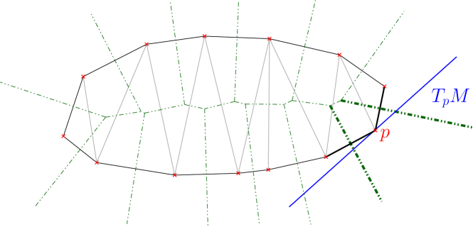
Figure 2: Construction of $\mathrm{Del}^{\omega}(\mathcal{P},T)$ at $p$ for $\omega\equiv 0$: $p$ has three incident edges in the ambient Delaunay triangulation, but only two (bold) have dual Voronoi face intersecting $T_{p}M$.

The weight assignment $\omega$ gives degrees of freedom for the reconstruction. The extra degree of freedom $\omega$ permits to stabilize the triangulation and to remove the so-called inconsistencies, the points remaining fixed. For further details, see [5, 4].

3.2 Guarantees

The following result sums up the reconstruction properties of the Tangential Delaunay Complex that we will use. For more details about it, the reader is referred to [4].

Theorem 10 (Theorem 5.3 in [4]).

There exists $\varepsilon_{d}>0$ such that for all $\varepsilon\leq\varepsilon_{d}\rho$ and all $M\in\mathcal{M}_{D,d,\rho}$, if $\mathcal{P}\subset M$ is an $(\varepsilon,2\varepsilon)$-net, there exists a weight assignment $\omega_{\ast}=\omega_{\ast\mathcal{P},T}$ depending on $\mathcal{P}$ and $T=\left\{T_{p}M\right\}_{p\in\mathcal{P}}$ such that

• ${d}_{H}\left(M,\mathrm{Del}^{\omega_{\ast}}(\mathcal{P},T)\right)\leq{C_{d}}{\varepsilon^{2}}/{\rho}$,

• $M$ and $\mathrm{Del}^{\omega_{\ast}}(\mathcal{P},T)$ are ambient isotopic.

Computing $\mathrm{Del}^{\omega_{\ast}}(\mathcal{P},T)$ requires to determine the weight function $\omega_{\ast}=\omega_{\ast\mathcal{P},T}$. In [4], a greedy algorithm is designed for this purpose and has a time complexity ${O}\left(Dn^{2}+D2^{O(d^{2})}n\right)$.

Given an $(\varepsilon,2\varepsilon)$-net $\mathcal{P}$ for $\varepsilon$ small enough, $\mathrm{Del}^{\omega_{\ast}}(\mathcal{P},T)$ recovers $M$ up to ambient isotopy and approximates it at the scale $\varepsilon^{2}$. The order of magnitude $\varepsilon^{2}$ with an input $\mathcal{P}$ of scale $\varepsilon$ is remarkable. Another instance of this phenomenon is present in [13] in codimension $1$. We will show that this $\varepsilon^{2}$ provides the minimax rate of approximation when dealing with random samples. Therefore, it can be thought of as optimal.

Theorem 10 suffers two major imperfections. First, it requires the knowledge of the tangent spaces at each sample point — since ${\omega_{\ast}}={\omega_{\ast\mathcal{P},T}}$ — and it is no longer usable if tangent spaces are only known up to some error. Second, the points are assumed to lie exactly on the submanifold $M$, and no noise is allowed. The analysis of $\mathrm{Del}^{\omega_{\ast}}(\mathcal{P},T)$ is sophisticated [4]. Rather than redo the whole study with milder assumptions, we tackle this question with an approximation theory approach (Theorem 11). Instead of studying if $\mathrm{Del}^{\omega_{\ast}}(\mathcal{P}^{\prime},T^{\prime})$ is stable when $\mathcal{P}^{\prime}$ lies close to $M$ and $T^{\prime}$ close to $T$, we examine what $\mathrm{Del}^{\omega_{\ast}}(\mathcal{P}^{\prime},T^{\prime})$ actually reconstructs, as detailed in Section 4.

3.3 On the Sparsity Assumption

In Theorem 10, $\mathcal{P}$ is assumed to be dense enough so that it covers all the areas of $M$. It is also supposed to be sparse at the same scale as the density parameter $\varepsilon$. Indeed, arbitrarily accumulated points would generate non-uniformity and instability for $\mathrm{Del}^{\omega_{\ast}}(\mathcal{P},T)$ [5, 4]. At this stage, we emphasize that the construction of a $(\varepsilon,2\varepsilon)$-net can be carried out given an $\varepsilon$-dense sample. Given an $\varepsilon$-dense sample $\mathcal{P}$, the farthest point sampling algorithm prunes $\mathcal{P}$ and outputs an $(\varepsilon,2\varepsilon)$-net $\mathcal{Q}\subset\mathcal{P}$ of $M$ as follows. Initialize at $\mathcal{Q}=\{p_{1}\}\subset\mathcal{P}$, and while $\underset{p\in\mathcal{P}}{\max}~{}{d}(p,\mathcal{Q})>\varepsilon$, add to $\mathcal{Q}$ the farthest point to $\mathcal{Q}$ in $\mathcal{P}$, that is, $\mathcal{Q}\leftarrow\mathcal{Q}\cup\{\underset{p\in\mathcal{P}}{\operatornamewithlimits{argmax}}~{}{d}(p,\mathcal{Q})\}$. The output $\mathcal{Q}$ is $\varepsilon$-sparse and satisfies ${d}_{H}(\mathcal{P},\mathcal{Q})\leq\varepsilon$, so it is a $(\varepsilon,2\varepsilon)$-net of $M$. Therefore, up to the multiplicative constant $2$, sparsifying $\mathcal{P}$ at scale $\varepsilon$ will not deteriorate its density property. Then, we can run the farthest point sampling algorithm to preprocess the data, so that the obtained point cloud is a net.

4 Stability Result

4.1 Interpolation Theorem

As mentioned above, if the data do not lie exactly on $M$ and if we do not have the exact knowledge of the tangent spaces, Theorem 10 does not apply. To bypass this issue, we interpolate the data with another submanifold $M^{\prime}$ satisfying good properties, as stated in the following result.

Theorem 11 (Interpolation).

Let $M\in\mathcal{M}_{D,d,\rho}$. Let $\mathcal{P}=\{p_{1},\ldots,p_{q}\}\subset\mathbb{R}^{D}$ be a finite point cloud and $\tilde{T}=\left\{\tilde{T}_{1},\ldots,\tilde{T}_{q}\right\}$ be a family of $d$-dimensional linear subspaces of $\mathbb{R}^{D}$. For $\theta\leq\pi/64$ and $18\eta<\delta\leq\rho$, assume that

• $\mathcal{P}$ is $\delta$-sparse: $\underset{i\neq j}{\min}\left\|p_{j}-p_{i}\right\|\geq\delta$,

• the $p_{j}$’s are $\eta$-close to $M$: $\underset{1\leq j\leq q}{\max}{d}(p_{j},M)\leq\eta$,

• $\underset{1\leq j\leq q}{\max}\>\angle(T_{\pi_{M}(p_{j})}M,\tilde{T}_{j})\leq\sin\theta$.

Then, there exist a universal constant $c_{0}\leq 285$ and a compact $d$-dimensional connected submanifold $M^{\prime}\subset\mathbb{R}^{D}$ without boundary such that

1. $\mathcal{P}\subset M^{\prime}$,

2. $\mathrm{reach}\bigl{(}M^{\prime}\bigr{)}\geq\left(1-c_{0}\left(\frac{\eta}{\delta}+{\theta}\right)\frac{\rho}{\delta}\right)\rho,$

3. $T_{p_{j}}M^{\prime}=\tilde{T}_{j}$ for all $1\leq j\leq q$,

4. ${d}_{H}(M,M^{\prime})\leq\delta\theta+\eta$,

5. $M$ and $M^{\prime}$ are ambient isotopic.

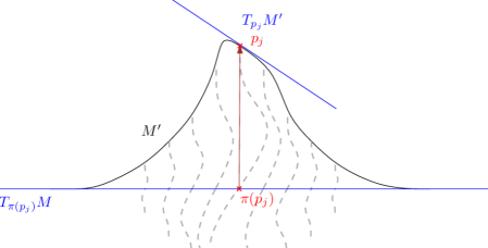
Figure 3: An instance of the interpolating submanifold $M^{\prime}$. Dashed lines correspond to the image of vertical lines by the ambient diffeomorphism $\Phi$ defining $M^{\prime}=\Phi(M)$.

Theorem 11 fits a submanifold $M^{\prime}$ to noisy points and perturbed tangent spaces with no change of topology and a controlled reach loss. We will use $M^{\prime}$ as a proxy for $M$. Indeed, if $\tilde{T}_{1},\ldots,\tilde{T}_{q}$ are estimated tangent spaces at the noisy base points $p_{1},\ldots,p_{q}$, $M^{\prime}$ has the virtue of being reconstructed by $\mathrm{Del}^{\omega_{\ast}}(\mathcal{P},\tilde{T})$ from Theorem 10. Since $M^{\prime}$ is topologically and geometrically close to $M$, we conclude that $M$ is reconstructed as well by transitivity. In other words, Theorem 11 allows to consider a noisy sample with estimated tangent spaces as an exact sample with exact tangent spaces. $M^{\prime}$ is built pushing and rotating $M$ towards the $p_{j}$’s locally along the vector $\left(p_{j}-\pi(p_{j}\right))$, as illustrated in Figure 3. Since the construction is quite general and may be applied in various settings, let us provide an outline of the construction.

Let $\phi(x)=\exp\bigl{(}\frac{\left\|x\right\|^{2}}{\left\|x\right\|^{2}-1}\bigr{)}\mathbbm{1}_{\left\|x\right\|^{2}<1}$. $\phi$ is smooth and satisfies $\phi(0)=1$, $\left\|\phi\right\|_{\infty}\leq 1$ and ${d}_{0}\phi=0$. For $j=1,\ldots,q$, it follows easily from the definition of $\angle(T_{\pi(p_{j})}M,\tilde{T}_{j})$ — e.g. by induction on the dimension — that there exists a rotation $R_{j}$ of $\mathbb{R}^{D}$ mapping $T_{\pi(p_{j})}M$ onto $\tilde{T}_{j}$ that satisfies $\left\|R_{j}-I_{D}\right\|_{op}\leq 2\sin\left(\theta/2\right)\leq\theta$. For $\ell>0$ to be chosen later, and all $a\in\mathbb{R}^{D}$, let us define $\Phi:\mathbb{R}^{D}\rightarrow\mathbb{R}^{D}$ by

$$\Phi(a) =a+\sum_{j=1}^{q}\phi\left(\frac{a-\pi(p_{j})}{\ell}\right)\bigl{[}\underbrace{(R_{j}-I_{D})(a-\pi(p_{j}))+(p_{j}-\pi(p_{j}))}_{\psi_{j}(a)}\bigr{]}.$$

$\Phi$ is designed to map $\pi(p_{j})$ onto $p_{j}$ with ${d}_{\pi(p_{j})}\Phi=R_{j}$. Roughly speaking, in balls of radii $\ell$ around each $\pi(p_{j})$, $\Phi$ shifts the points in the direction $p_{j}-\pi(p_{j})$ and rotates it around $\pi(p_{j})$. Off these balls, $\Phi$ is the identity map. To guarantee smoothness, the shifting and the rotation are modulated by the kernel $\phi$, as $\left\|a-\pi(p_{j})\right\|$ increases. Notice that ${d}_{a}\psi_{j}=(R_{j}-I_{D})$ and $\left\|\psi_{j}(a)\right\|\leq\ell\theta+\eta$ whenever $\phi\left(\frac{a-\pi(p_{j})}{\ell}\right)\neq 0$. Defining $M^{\prime}=\Phi(M)$, the facts that $M^{\prime}$ fits to $\mathcal{P}$ and $\tilde{T}$ and is Hausdorff-close to $M$ follow by construction. Moreover, Theorem 4.19 of [22] (reproduced as Lemma 24 in this paper) states that the reach is stable with respect to $\mathcal{C}^{2}$-diffeomorphisms of the ambient space. The estimate on $\mathrm{reach}(M^{\prime})$ relies on the following lemma stating differentials estimates on $\Phi$.

Lemma 12.

There exist universal constants $C_{1}\leq 7/2$ and $C_{2}\leq 28$ such that if $6\eta<\ell\leq\delta/3$ and $\theta\leq\pi/64$, $\Phi:\mathbb{R}^{D}\longrightarrow\mathbb{R}^{D}$ is a global $\mathcal{C}^{\infty}$-diffeomorphism. In addition, for all $a$ in $\mathbb{R}^{D}$,

$$\left\|{d}_{a}\Phi\right\|_{\mathrm{op}}\leq 1+C_{1}\left(\frac{\eta}{\ell}+\theta\right),~{}~{}\left\|{d}_{a}\Phi^{-1}\right\|_{\mathrm{op}}\leq\frac{1}{1-C_{1}\left(\frac{\eta}{\ell}+\theta\right)},~{}~{}\left\|{d}^{2}_{a}\Phi\right\|_{\mathrm{op}}\leq C_{2}\left(\frac{\eta}{\ell^{2}}+\frac{\theta}{\ell}\right).$$

The ambient isotopy follows easily by considering the weighted version $\Phi_{(t)}(a)=a+t\left(\Phi(a)-a\right)$ for $0\leq t\leq 1$ and the same differential estimates. We then take the maximum possible value $\ell=\delta/3$ and $M^{\prime}=\Phi(M)$.

Remark 13.

Changing slightly the construction of $M^{\prime}$, one can also build it such that the curvature tensor at each $p_{j}$ corresponds to that of $M$ at $\pi(p_{j})$. For this purpose it suffices to take a localizing function $\phi$ identically equal to $1$ in a neighborhood of $0$. This additional condition would impact the universal constant $c_{0}$ appearing in Theorem 11.

4.2 Stability of the Tangential Delaunay Complex

Theorem 11 shows that even in the presence of noisy sample points at distance $\eta$ from $M$, and with the knowledge of the tangent spaces up to some angle $\theta$, it is still possible to apply Theorem 10 to some virtual submanifold ${M}^{\prime}$. Denoting $\tilde{M}=\mathrm{Del}^{\omega_{\ast}}(\mathcal{P},\tilde{T})$, since ${d}_{H}(M,\tilde{M})\leq{d}_{H}(M,M^{\prime})+{d}_{H}(M^{\prime},\tilde{M})$ and since the ambient isotopy relation is transitive, $M\cong M^{\prime}\cong\tilde{M}$. We get the following result as a straightforward combination of Theorem 10 and Theorem 11.

Theorem 14 (Stability of the Tangential Delaunay Complex).

There exists $\varepsilon_{d}>0$ such that for all $\varepsilon\leq\varepsilon_{d}\rho$ and all $M\in\mathcal{M}_{D,d,\rho}$, the following holds. Let $\mathcal{P}\subset\mathbb{R}^{D}$ finite point cloud and $\tilde{T}=\left\{\tilde{T}_{p}\right\}_{p\in\mathcal{P}}$ be a family of $d$-dimensional linear subspaces of $\mathbb{R}^{D}$ such that

• $\underset{p\in\mathcal{P}}{\max}\>{d}(p,M)\leq\eta$,

• $\underset{p\in\mathcal{P}}{\max}\>\angle(T_{\pi_{M}(p)}{M},\tilde{T}_{p})\leq\sin\theta$,

• $\mathcal{P}$ is $\varepsilon$-sparse,

• $\underset{x\in M}{\max}\>{d}(x,\mathcal{P})\leq 2\varepsilon$.

If $\theta\leq\varepsilon/(1140\rho)$ and $\eta\leq\varepsilon^{2}/(1140\rho)$, then,

• ${d}_{H}\left(M,\mathrm{Del}^{\omega_{\ast}}(\mathcal{P},\tilde{T})\right)\leq C_{d}\varepsilon^{2}/\rho$,

• $M$ and $\mathrm{Del}^{\omega_{\ast}}(\mathcal{P},\tilde{T})$ are ambient isotopic.

Indeed, applying the reconstruction algorithm of Theorem 10 even in the presence of noise and uncertainty on the tangent spaces actually recovers the submanifold $M^{\prime}$ built in Theorem 11. $M^{\prime}$ is isotopic to $M$ and the quality of the approximation of $M$ is at most impacted by the term ${d}_{H}(M,M^{\prime})\leq\varepsilon\theta+\eta$. The lower bound on $\mathrm{reach}(M^{\prime})$ is crucial, as constants appearing in Theorem 10 are not bounded for arbitrarily small reach.

It is worth noting that no extra analysis of the Tangential Delaunay Complex was needed to derive its stability. The argument is global, constructive, and may be applied to other reconstruction methods taking tangent spaces as input. For instance, a stability result similar to Theorem 14 could be derived readily for the so-called cocone complex [12] using the interpolating submanifold of Theorem 11.

5 Tangent Space Estimation and Decluttering Procedure

5.1 Additive Noise Case

We now focus on the estimation of tangent spaces in the model with additive noise $\mathcal{G}_{D,d,f_{min},f_{max},\rho,\sigma}$. The proposed method is similar to that of [2, 28]. A point $p\in M$ being fixed, $T_{p}M$ is the best local $d$-dimensional linear approximation of $M$ at $p$. Performing a Local Principal Component Analysis (PCA) in a neighborhood of $p$ is likely to recover the main directions spanned by $M$ at $p$, and therefore yield a good approximation of $T_{p}M$. For $j=1,\ldots,n$ and $h>0$ to be chosen later, define the local covariance matrix at $X_{j}$ by

$$\hat{\Sigma}_{j}(h)=\frac{1}{n-1}\sum_{i\neq j}\left(X_{i}-\bar{X}_{j}\right)\left(X_{i}-\bar{X}_{j}\right)^{t}\mathbbm{1}_{\mathcal{B}(X_{j},h)}(X_{i}),$$

where $\bar{X}_{j}=\frac{1}{N_{j}}\sum_{i\neq j}{X_{i}\mathbbm{1}_{\mathcal{B}(X_{j},h)}(X_{i})}$ is the barycenter of sample points contained in the ball $\mathcal{B}(X_{j},h)$, and $N_{j}=|\mathcal{B}(X_{j},h)\cap\mathbb{X}_{n}|$. Let us emphasize the fact that the normalization $1/(n-1)$ in the definition of $\hat{\Sigma}_{j}$ stands for technical convenience. In fact, any other normalization would yield the same guarantees on tangent spaces since only the principal directions of $\hat{\Sigma}_{j}$ play a role. Set $\hat{T}_{j}(h)$ to be the linear space spanned by the $d$ eigenvectors associated with the $d$ largest eigenvalues of $\hat{\Sigma}_{j}(h)$. Computing a basis of $\hat{T}_{j}(h)$ can be performed naively using a singular value decomposition of the full matrix $\hat{\Sigma}_{j}(h)$, although fast PCA algorithms [31] may lessen the computational dependence on the ambient dimension. We also denote by $\mathtt{TSE}(.,h)$ the function that maps any vector of points to the vector of their estimated tangent spaces, with

$$\hat{T}_{j}(h)=\mathtt{TSE}(\mathbb{X}_{n},h)_{j}.$$

Proposition 15.

Set $h=\left(c_{d,f_{min},f_{max}}\frac{\log n}{n-1}\right)^{1/d}$ for $c_{d,f_{min},f_{max}}$ large enough. Assume that $\sigma/h\leq 1/4$. Then for $n$ large enough, for all $Q\in\mathcal{G}_{D,d,f_{min},f_{max},\rho,\sigma}$,

$$\max_{1\leq j\leq n}\angle\left(T_{\pi_{M}(X_{j})}{M},\hat{T}_{j}(h)\right)\leq C_{d,f_{min},f_{max}}\left(\frac{h}{\rho}+\frac{\sigma}{h}\right),$$

with probability larger than $1-4\left(\frac{1}{n}\right)^{\frac{2}{d}}$.

An important feature given by Proposition 15 is that the statistical error of our tangent space estimation procedure does not depend on the ambient dimension $D$. The intuition behind Proposition 15 is the following: if we assume that the true tangent space $T_{X_{j}}M$ is spanned by the first $d$ vectors of the canonical basis, we can decompose $\hat{\Sigma}_{j}$ as

$$\hat{\Sigma}_{j}(h)=\left(\begin{array}[]{@{}c|c}\hat{A}_{j}(h)&0\\ \hline\cr 0&0\end{array}\right)+\hat{R},$$

where $\hat{R}$ comes from the curvature of the submanifold along with the additive noise, and is of order $N_{j}(h)(h^{3}/(\rho(n-1))+h\sigma)\lesssim h^{d+2}(h/\rho+\sigma/h)$, provided that $h$ is roughly smaller than $(\log(n)/(n-1))^{1/d}$. On the other hand, for a bandwidth $h$ of order $(\log(n)/(n-1))^{1/d}$, $\hat{A}_{j}(h)$ can be proved (Lemma 36) to be close to its deterministic counterpart

$$A_{j}(h)=\mathbb{E}\left(\left(\pi_{T_{X_{j}}M}(X)-\mathbb{E}\pi_{T_{X_{j}}M}(X)\right)\left(\pi_{T_{X_{j}}M}(X)-\mathbb{E}\pi_{T_{X_{j}}M}(X)\right)^{t}\mathbbm{1}_{\mathcal{B}(X_{j},h)}(X)\right),$$

where $\pi_{T_{X_{j}}M}$ denotes orthogonal projection onto $T_{X_{j}}M$ and expectation is taken conditionally on $X_{j}$. The bandwidth $(\log(n)/(n-1))^{1/d}$ may be thought of as the smallest radius that allows enough sample points in balls to provide an accurate estimation of the covariance matrices. Then, since $f_{min}>0$, Lemma 35 shows that the minimum eigenvalue of $A(h)$ is of order $h^{d+2}$. At last, an eigenvalue perturbation result (Proposition 38) shows that $\hat{T}_{j}(h)$ must be close to $T_{X_{j}}M$ up to $(h^{d+3}/\rho+h^{d+1}\sigma)/(h^{d+2})\approx h/\rho+\sigma/h$. The complete derivation is provided in Section E.1.

Then, it is shown in Lemma 32, based on the results of [11], that letting $\varepsilon=c_{d,f_{min},f_{max}}(h\vee\rho\sigma/h)$ for $c_{d,f_{min},f_{max}}$ large enough, entails $\mathbb{X}_{n}$ is $\varepsilon$-dense in $M$ with probability larger than $1-\left(\frac{1}{n}\right)^{2/d}$. Since $\mathbb{X}_{n}$ may not be sparse at the scale $\varepsilon$, and for the stability reasons described in Section 3, we sparsify it with the farthest point sampling algorithm (Section 3.3) with scale parameter $\varepsilon$. Let $\mathbb{Y}_{n}$ denote the output of the algorithm. If $\sigma\leq h/4$, and $c_{d,f_{min},f_{max}}$ is large enough, we have the following.

Corollary 16.

With the above notation, for $n$ large enough, with probability at least $1-5\left(\frac{1}{n}\right)^{2/d}$,

• $\underset{X_{j}\in\mathbb{Y}_{n}}{\max}\>{d}(X_{j},M)\leq\frac{\varepsilon^{2}}{1140\rho}$,

• $\underset{X_{j}\in\mathbb{Y}_{n}}{\max}\angle(T_{\pi_{M}(X_{j})}{M},\hat{T}_{j}(h))\leq\frac{\varepsilon}{2280\rho}$,

• $\mathbb{Y}_{n}$ is $\varepsilon$-sparse,

• $\underset{x\in M}{\max}\>{d}(x,\mathbb{Y}_{n})\leq 2\varepsilon$.

In other words, the previous result shows that $\mathbb{Y}_{n}$ satisfies the assumptions of Theorem 14 with high probability. We may then define $\hat{M}_{\mathtt{TDC}}$ to be the Tangential Delaunay Complex computed on $\mathbb{Y}_{n}$ and the collection of estimated tangent spaces $\mathtt{TSE}(\mathbb{X}_{n},h)_{\mathbb{Y}_{n}}$, that is elements of $\mathtt{TSE}(\mathbb{X}_{n},h)$ corresponding to elements of $\mathbb{Y}_{n}$, where $h$ is the bandwidth defined in Proposition 15.

Definition 17.

With the above notation, define $\hat{M}_{\mathtt{TDC}}=\mathrm{Del}^{\omega_{\ast}}\left(\mathbb{Y}_{n},\mathtt{TSE}(\mathbb{X}_{n},h)_{\mathbb{Y}_{n}}\right)$.

Combining Theorem 14 and Corollary 16, it is clear that $\hat{M}_{\mathtt{TDC}}$ satisfies Theorem 7.

5.2 Clutter Noise Case

Let us now focus on the model with outliers $\mathcal{O}_{D,d,f_{min},f_{max},\rho,\beta}$. We address problem of decluttering the sample $\mathbb{X}_{n}$, that is, to remove outliers. We follow ideas from [24]. To distinguish whether $X_{j}$ is an outlier or belongs to $M$, we notice again that points drawn from $M$ approximately lie on a low dimensional structure. On the other hand, the neighborhood points of an outlier drawn far away from $M$ should typically be distributed in an isotropic way. Let $k_{1},k_{2},h>0$, $x\in\mathbb{R}^{D}$ and $T\subset\mathbb{R}^{D}$ a $d$-dimensional linear subspace. The slab at $x$ in the direction $T$ is the set $S(x,T,h)=\left\{x\right\}\oplus\mathcal{B}_{T}\left(0,k_{1}h\right)\oplus\mathcal{B}_{T^{\perp}}\!\left(0,k_{2}h^{2}\right)\subset\mathbb{R}^{D}$, where $\oplus$ denotes the Minkovski sum, and $\mathcal{B}_{T},\mathcal{B}_{T^{\perp}}$ are the Euclidean balls in $T$ and $T^{\perp}$ respectively.

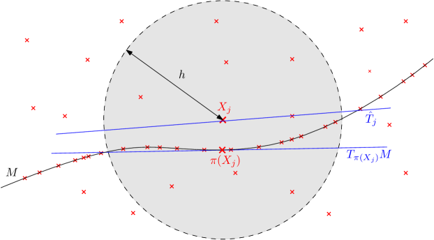
Figure 4: Local PCA at an outlier point $X_{j}\in\mathbb{X}_{n}$.

Following notation of Section 2.1, for $P\in\mathcal{O}_{D,d,f_{min},f_{max},\rho,\beta}$, let us write $P=\beta Q+(1-\beta)U_{\mathcal{B}_{0}}$. For $h$ small enough, by definition of the slabs, $U_{\mathcal{B}_{0}}\left(S(x,T_{\pi(x)}M,h)\right)\asymp(k_{1}h)^{d}(k_{2}h^{2})^{D-d}\asymp h^{2D-d}$. Furthermore, Figure 5 indicates that for $k_{1}$ and $k_{2}$ small enough, $Q\left(S(x,T_{\pi(x)}M,h)\right)\asymp Vol\left(S(x,T_{\pi(x)}M,h)\cap M\right)\asymp h^{d}$ if ${d}(x,M)\leq h^{2}$, and $Q\left(S(x,T_{\pi(x)}M,h)\right)=0$ if ${d}(x,M)>h^{2}$. Coming back to $P=\beta Q+(1-\beta)U_{\mathcal{B}_{0}}$, we roughly get

$$\begin{array}[]{@{}lcclrc}P\left(S(x,T_{\pi(x)}M,h)\right)\asymp&\beta h^{d}&+(1-\beta)h^{2D-d}&\asymp h^{d}&\text{~{}if~{}}&{d}(x,M)\leq h^{2},\\ P\left(S(x,T_{\pi(x)}M,h)\right)\asymp&0&+(1-\beta)h^{2D-d}&\asymp h^{2D-d}&\text{~{}if~{}}&{d}(x,M)>h^{2},\end{array}$$

as $h$ goes to $0$, for $k_{1}$ and $k_{2}$ small enough. Since $h^{2D-d}\ll h^{d}$, the measure $P\left(S(x,T,h)\right)$ of the slabs clearly is discriminatory for decluttering, provided that tangent spaces are known.

Based on this intuition, we define the elementary step of our decluttering procedure as the map $\mathtt{SD}_{t}(.,.,h)$, that sends a vector $P=\left(p_{1},\ldots,p_{r}\right)\subset\mathbb{R}^{D}$ and a corresponding vector of (estimated) tangent spaces $T_{\mathcal{P}}=(T_{1},\ldots,T_{r})$ onto a subvector of $\mathcal{P}$ according to the rule

$$p_{j}\in\mathtt{SD}_{t}(\mathcal{P},T_{\mathcal{P}},h)\quad\Leftrightarrow\quad|S(p_{j},T_{j},h)\cap\mathcal{P}|\geq t(n-1)h^{d},$$

where $t$ is a threshold to be fixed. This procedure relies on counting how many sample points lie in the slabs of direction the estimated tangent spaces (see Figure 5).

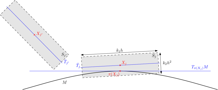
Figure 5: The slab $S(X_{j},\hat{T}_{j},h)$ is centered at $X_{j}$ and has size $k_{1}h$ in the $d$ directions spanned by $\hat{T}_{j}$, and size $k_{2}h^{2}$ in the $D-d$ directions normal to $\hat{T}_{j}$.

Since tangent spaces are unknown, the following result gives some insight on the relation between the accuracy of the tangent space estimation and the decluttering performance that can be reached.

Lemma 18.

Let $K>0$ be fixed. There exist constants $k_{1}(K)$ and $k_{2}(\rho,K)$ such that for every $h\leq 1$ and $x$ in $\mathbb{R}^{D}$, $S(x,T,h)\subset\mathcal{B}(x,h/2)$. Moreover, for every $h\leq h_{+}\wedge 1$ we have

$$\begin{array}[]{@{}ccc}h/\sqrt{2}\geq{d}(x,M)\geq h^{2}/\rho\quad\mbox{and}\quad\angle\left(T_{\pi_{M}(x)}M,T\right)\leq Kh/\rho&\Rightarrow&S(x,T,h)\subset S^{\prime}(x,T_{\pi_{M}(x)}M,h),\end{array}$$

where $S^{\prime}(x,T_{\pi_{M}(x)}M,h)$ is a larger slab with parameters $k^{\prime}_{1}(\rho,K)$ and $k^{\prime}_{2}(\rho,K)$, which are such that $S^{\prime}(x,T_{\pi_{M}(x)}M,h)\cap M=\emptyset$. In addition, there exists $k_{3}(\rho,K)$ such that for all $x$ and $y$ are in $M$,

$$\angle\left(T_{x}M,T\right)\leq Kh/\rho\quad\mbox{and}\quad\left\|x-y\right\|\leq k_{3}h\quad\Rightarrow\quad y\in S(x,T,h).$$

Possible values for $k_{1}$ and $k_{2}$ are, respectively, $\frac{1}{16(K\vee 1)}$ and $\frac{1}{16(\rho\vee K\vee 1)}$, and $k_{3}$ can be taken as $k_{1}\wedge\frac{\rho k_{2}}{1+2K}$.

The proof of Lemma 18, mentioned in [24], follows from elementary geometry, combined with the definition of the reach and Proposition 25.

Roughly, Lemma 18 states that the decluttering performance is of order the square of the tangent space precision, hence will be closely related to the performance of the tangent space estimation procedure $\mathtt{TSE}$. Unfortunately, a direct application of $\mathtt{TSE}$ to the corrupted sample $\mathbb{X}_{n}$ leads to slightly worse precision bounds, in terms of angle deviation. Typically, the angle deviation would be of order $n^{-1/(d+1)}$. However, this precision is enough to remove outliers points which are at distance at least $n^{-2/(d+1)}$ from $M$. Then running our $\mathtt{TSE}$ on this refined sample $\mathtt{SD}_{t}(\mathbb{X}_{n},\mathtt{TSE}(\mathbb{X}_{n}),n^{-1/(d+1)})$ leads to better angle deviation rates, hence better decluttering performance, and so on.

Let us introduce an iterative decluttering procedure in a more formal way. We choose the initial bandwidth $h_{0}=\left(c_{d,f_{min},f_{max},\rho}\frac{\log n}{\beta(n-1)}\right)^{\gamma_{0}}$, with $\gamma_{0}=1/(d+1)$, and define the first set $\mathbb{X}^{(-1)}=\mathbb{X}_{n}$ as the whole sample. We then proceed recursively, setting $h_{k+1}=\left(c_{d,f_{min},f_{max},\rho}\frac{\log n}{\beta(n-1)}\right)^{\gamma_{k+1}}$, with $\gamma_{k+1}$ satisfying $\gamma_{k+1}=(2\gamma_{k}+1)/(d+2)$. This recursion formula is driven by the optimization of a trade-off between imprecision terms in tangent space estimation, as may be seen from (10). An elementary calculation shows that

$$\gamma_{k}=\frac{1}{d}-\frac{1}{d(d+1)}\left(\frac{2}{d+2}\right)^{k}.$$

With this updated bandwidth we define

$$\mathbb{X}^{(k+1)}=\mathtt{SD}_{t}(\mathbb{X}^{(k)},\mathtt{TSE}(\mathbb{X}^{(k)},h_{k+1}),h_{k+1}).$$

In other words, at step $k+1$ we use a smaller bandwidth $h_{k+1}$ in the tangent space estimation procedure $\mathtt{TSE}$. Then we use this better estimation of tangent spaces to run the elementary decluttering step $\mathtt{SD}$. The performance of this procedure is guaranteed by the following proposition. With a slight abuse of notation, if $X_{j}$ is in $\mathbb{X}^{(k)}$, $\mathtt{TSE}(\mathbb{X}^{(k)},h)_{j}$ will denote the corresponding tangent space of $\mathtt{TSE}(\mathbb{X}^{(k)},h)$.

Proposition 19.

In the clutter noise model, for $t$, $c_{d,f_{min},f_{max},\rho}$ and $n$ large enough, $k_{1}$ and $k_{2}$ small enough, the following properties hold with probability larger than $1-7\left(\frac{1}{n}\right)^{2/d}$ for all $k\geq 0$.

Initialization:

• For all $X_{j}$ $\in$ $\mathbb{X}^{(-1)}$ such that ${d}(X_{j},M)\leq h_{0}/\sqrt{2}$,

  $$\angle\bigl{(}\mathtt{TSE}(\mathbb{X}^{(-1)},h_{0})_{j},T_{\pi(X_{j})}{M}\bigr{)}\leq C_{d,f_{min},f_{max}}h_{0}/\rho.$$

• For every $X_{j}$ $\in$ $M\cap\mathbb{X}^{(-1)}$, $X_{j}$ $\in$ $\mathbb{X}^{(0)}$.

• For every $X_{j}$ $\in$ $\mathbb{X}^{(-1)}$, if ${d}(X_{j},M)>h_{0}^{2}/\rho$, then $X_{j}$ $\notin$ $\mathbb{X}^{(0)}$.

Iterations:

• For all $X_{j}$ $\in$ $\mathbb{X}^{(k)}$ such that ${d}(X_{j},M)\leq h_{k+1}/\sqrt{2}$,

  $$\angle\bigl{(}\mathtt{TSE}(\mathbb{X}^{(k)},h_{k+1})_{j},T_{\pi(X_{j})}{M}\bigr{)}\leq C_{d,f_{min},f_{max}}h_{k+1}/\rho.$$

• For every $X_{j}$ $\in$ $M\cap\mathbb{X}^{(k)}$, $X_{j}$ $\in$ $\mathbb{X}^{(k+1)}$.

• For every $X_{j}$ $\in$ $\mathbb{X}^{(k)}$, if ${d}(X_{j},M)>h_{k+1}^{2}/\rho$, then $X_{j}$ $\notin$ $\mathbb{X}^{(k+1)}$.

This result is threefold. Not only can we distinguish data and outliers within a decreasing sequence of offsets of radii $h_{k}^{2}/\rho$ around $M$, but we can also ensure that no point of $M$ is removed during the process with high probability. Moreover, it also provides a convergence rate for the estimated tangent spaces $\mathtt{TSE}(\mathbb{X}_{k},h_{k+1})$.

Now fix a precision level $\delta$. If $k$ is larger than $(\log(1/\delta)-\log(d(d+1))/(\log(d+2)-\log(2))$, then $1/d>\gamma_{k}\geq 1/d-\delta$. Let us define $k_{\delta}$ as the smallest integer satisfying $\gamma_{k}\geq 1/d-\delta$, and denote by $\mathbb{Y}_{n}^{\delta}$ the output of the farthest point sampling algorithm applied to $\mathbb{X}^{(k_{\delta})}$ with parameter $\varepsilon=c_{d,f_{min}f_{max}}h_{k_{\delta}}$, for $c_{d,f_{min}f_{max}}$ large enough. Define also $\hat{T}^{\delta}$ as the restriction of $\mathtt{TSE}(\mathbb{X}^{(k_{\delta})},h_{k_{\delta}})$ to the elements of $\mathbb{Y}_{n}^{\delta}$.

According to Proposition 19, the decluttering procedure removes no data point on $M$ with high probability. In other words, $\mathbb{X}^{(k_{\delta})}\cap M=\mathbb{X}_{n}\cap M$, and as a consequence, $\underset{x\in M}{\max}\>{d}(x,\mathbb{X}^{(k_{\delta})})\leq c_{d,f_{min}}\left(\frac{\log n}{\beta n}\right)^{1/d}\ll h_{k_{\delta}}$ with high probability (see Lemma 32). As a consequence, we obtain the following.

Corollary 20.

With the above notation, for $n$ large enough, with probability larger than $1-8\left(\frac{1}{n}\right)^{2/d}$,

• $\underset{X_{j}\in\mathbb{Y}_{n}^{\delta}}{\max}{d}(X_{j},M)\leq\frac{\varepsilon^{2}}{1140\rho}$,

• $\underset{X_{j}\in\mathbb{Y}_{n}^{\delta}}{\max}\angle(T_{\pi_{M}(X_{j})}{M},\hat{T}^{\delta}_{j})\leq\frac{\varepsilon}{2280\rho}$,

• $\mathbb{Y}_{n}^{\delta}$ is $\varepsilon$-sparse,

• $\underset{x\in M}{\max}\>{d}(x,\mathbb{Y}_{n}^{\delta})\leq 2\varepsilon$.

We are now able to define the estimator $\hat{M}_{\mathtt{TDC\delta}}$.

Definition 21.

With the above notation, define $\hat{M}_{\mathtt{TDC\delta}}=\mathrm{Del}^{\omega_{\ast}}\left(\mathbb{Y}^{\delta}_{n},\hat{T}^{\delta}\right).$

Combining Theorem 14 and Corollary 20, it is clear that $\hat{M}_{\mathtt{TDC\delta}}$ satisfies Theorem 8.

Finally, we turn to the asymptotic estimator $\hat{M}_{\mathtt{TDC+}}$. Set $h_{\infty}=\left(c_{d,f_{min},f_{max},\rho}\frac{\log n}{\beta(n-1)}\right)^{1/d}$, and let $\hat{k}$ denote the smallest integer such that $\min\{{d}(X_{j},M)|{d}(X_{j},M)>h_{\infty}^{2}/\rho\}>h_{\hat{k}}^{2}/\rho$. Since $\mathbb{X}_{n}$ is a (random) finite set, we can always find such a random integer $\hat{k}$ that provides a sufficient number of iterations to obtain the asymptotic decluttering rate. For this random iteration $\hat{k}$, we can state the following result.

Proposition 22.

Under the assumptions of Corollary 20, for every $X_{j}$ $\in$ $X^{(\hat{k}+1)}$, we have

$$\angle(\mathtt{TSE}(\mathbb{X}^{(\hat{k}+1)},h_{\infty})_{j},T_{\pi(X_{j})}{M})\leq C_{d,f_{min},f_{max}}h_{\infty}/\rho.$$

As before, taking $\mathbb{Y}_{n}^{+}$ as the result of the farthest point sampling algorithm based on $\mathbb{X}^{(\hat{k}+1)}$, and $T^{+}$ the vector of tangent spaces $\mathtt{TSE}(\mathbb{X}^{(\hat{k}+1)},h_{\infty})_{j}$ such that $\mathbb{X}^{(\hat{k}+1)}_{j}$ $\in$ $\mathbb{Y}_{n}^{+}$, we can construct our last estimator.

Definition 23.

With the above notation, define $\hat{M}_{\mathtt{TDC+}}=\mathrm{Del}^{\omega_{\ast}}\left(\mathbb{Y}^{+}_{n},T^{+}\right).$

In turn, Proposition 22 implies that $\hat{M}_{\mathtt{TDC+}}$ satisfies Theorem 9.

6 Conclusion

In this work, we gave results on explicit manifold reconstruction with simplicial complexes. We built estimators $\hat{M}_{\mathtt{TDC}}$, $\hat{M}_{\mathtt{TDC\delta}}$ and $\hat{M}_{\mathtt{TDC+}}$ in two statistical models. We proved minimax rates of convergence for the Hausdorff distance and consistency results for ambient isotopic reconstruction. Since $\hat{M}_{\mathtt{TDC}}$ is minimax optimal in the additive noise model for $\sigma$ small, and uses the Tangential Delaunay Complex of [4], the latter is proved to be optimal. Moreover, rates of [24] are proved to be achievable with simplicial complexes that are computable using existing algorithms. To prove the stability of the Tangential Delaunay Complex, a generic interpolation result was derived. In the process, a tangent space estimation procedure and a decluttering method both based on local PCA were studied.

In the model with outliers, the proposed reconstruction method achieves a rate of convergence that can be as close as desired to the minimax rate of convergence, depending on the number of iterations of the decluttering procedure. Though this procedure seems to be well adapted to our reconstuction scheme — which is based on tangent spaces estimation — we believe that it could be of interest in the context of other applications. Also, further investigation may be carried out to compare this decluttering procedure to existing ones [9, 19].

As briefly mentioned below Theorem 7, our approach is likely to be suboptimal in cases where noise level $\sigma$ is large. In such cases, with additional structure on the noise such as centered and independent from the source, other statistical procedures such as deconvolution [24] could be adapted to provide vertices to the Tangential Delaunay Complex. Tangential properties of deconvolution are still to be studied.

The effective construction of $\hat{M}_{TDC\delta}$ can be performed using existing algorithms. Namely, Tangential Delaunay Complex, farthest point sampling, local PCA and point-to-linear subspace distance computation for slab counting. A crude upper bound on the time complexity of a naive step-by-step implementation is

$$O\left(nD\left[2^{O(d^{2})}+\log(1/\delta)D(D+n)\right]\right),$$

since the precision $\delta$ requires no more than $\log\left(1/\delta\right)$ iterations of the decluttering procedure. It is likely that better complexity bounds may be obtained using more refined algorithms, such as fast PCA [31], that lessens the dependence on the ambient dimension $D$. An interesting development would be to investigate a possible precision/complexity tradeoff, as done in [3] for community detection in graphs for instance.

Even though Theorem 11 is applied to submanifold estimation, we believe it may be applied in various settings. Beyond its statement, the way that it is used is quite general. When intermediate objects (here, tangent spaces) are used in a procedure, this kind of proxy method can provide extensions of existing results to the case where these objects are only approximated.

As local PCA is performed throughout the paper, the knowledge of the bandwidth $h$ is needed for actual implementation. In practice its choice is a difficult question and adaptive selection of $h$ remains to be considered.

In the process, we derived rates of convergence for tangent space estimation. The optimality of the method will be the object of a future paper.

acknowledgements

We would like to thank Jean-Daniel Boissonnat, Frédéric Chazal, Pascal Massart, and Steve Oudot for their insight and the interest they brought to this work. We are also grateful to the reviewers whose comments helped enhancing substantially this paper.

This work was supported by ANR project TopData ANR-13-BS01-0008 and by the Advanced Grant of the European Research Council GUDHI (Geometric Understanding in Higher Dimensions). E. Aamari was supported by the Conseil régional d’Île-de-France under a doctoral allowance of its program Réseau de Recherche Doctoral en Mathématiques de l’Île-de-France (RDM-IdF).

Appendix A Interpolation Theorem

This section is devoted to prove the interpolation results of Section 4.1. For sake of completeness, let us state a stability result for the reach with respect to $\mathcal{C}^{2}$-diffeomorphisms.

Lemma 24 (Theorem 4.19 in [22]).

Let $A\subset\mathbb{R}^{D}$ with $\mathrm{reach}(A)\geq\rho>0$ and $\Phi:\mathbb{R}^{D}\longrightarrow\mathbb{R}^{D}$ is a $\mathcal{C}^{1}$-diffeomorphism such that $\Phi$,$\Phi^{-1}$, and ${d}\Phi$ are Lipschitz with Lipschitz constants $K$,$N$ and $R$ respectively, then

$$\mathrm{reach}(\Phi(A))\geq\dfrac{1}{(K\rho^{-1}+R)N^{2}}.$$

Writing $\phi_{\ell}(\cdot)=\phi(\cdot/\ell)$, we recall that ${\psi_{j}(a)}={(R_{j}-I_{D})(a-\pi(p_{j}))+(p_{j}-\pi(p_{j}))}$ and

$$\Phi(a) =a+\sum_{j=1}^{q}\phi_{\ell}\left(a-\pi(p_{j})\right)\psi_{j}(a).$$ (1)

Let us denote $b_{1}=\sup_{x}\left\|{d}_{x}\phi\right\|$, $b_{2}=\sup_{x}\left\|{d}^{2}_{x}\phi\right\|_{\mathrm{op}}$, and write $C_{1}=1+b_{1}$, $C_{2}=b_{2}+2b_{1}$. Straightforward computation yields $C_{1}\leq 7/2$ and $C_{2}\leq 28$.

of Lemma 12.

First notice that the sum appearing in (1) consists of at most one term. Indeed, since $\phi\equiv 0$ outside $\mathcal{B}(0,1)$, if $\phi_{\ell}\left(a-\pi(p_{j})\right)\neq 0$ for some $j\in\{1,\ldots,q\}$, then $\left\|a-\pi(p_{j})\right\|\leq\ell$. Consequently, for all $i\neq j$,

$$\left\|a-\pi(p_{i})\right\| \geq\left\|p_{j}-p_{i}\right\|-\left\|p_{j}-\pi(p_{j})\right\|-\left\|\pi(p_{j})-a\right\|-\left\|\pi(p_{i})-p_{i}\right\|$$

$$\geq\delta-\eta-\ell-\eta$$

$$\geq\delta-2\ell\geq\ell,$$

where we used that $6\eta\leq\ell\leq\delta/3$. Therefore, $\phi_{\ell}\left(a-\pi(p_{i})\right)=0$ for all $i\neq j$. In other words, if a $p_{j}$ actually appears in $\Phi(a)$ then the others do not.

Global diffeomorphism: As the sum in (1) is at most composed of one term, chain rule yields

$$\left\|{d}_{a}\Phi-{{I_{D}}}\right\|_{\mathrm{op}} =\underset{1\leq j\leq q}{\max}\left\|{d}_{a}\left[\phi_{\ell}\left(a-\pi(p_{j})\right)\psi_{j}(a)\right]\right\|_{\mathrm{op}}$$

$$=\underset{1\leq j\leq q}{\max}\left\|\psi_{j}(a)\left.\frac{{d}_{b}\phi}{\ell}\right|_{b=\frac{a-\pi(p_{j})}{\ell}}+\phi_{\ell}\left(a-\pi(p_{j})\right)(R_{j}-I_{D})\right\|_{\mathrm{op}}$$

$$\leq\bigl{(}b_{1}+1\bigr{)}\theta+b_{1}\frac{\eta}{\ell}<1,$$

where the last line follows from $b_{1}\leq 5/2$, $6\eta\leq\ell$ and $\theta\leq\pi/64$. Therefore, ${d}_{a}\Phi$ is invertible for all $a\in\mathbb{R}^{D}$, and $\left({d}_{a}\Phi\right)^{-1}=\sum_{i=0}^{\infty}\left(I_{D}-{d}_{a}\Phi\right)^{i}$. $\Phi$ is a local diffeomorphism according to the local inverse function theorem. Moreover, $\left\|\Phi(a)\right\|\rightarrow\infty$ as $\left\|a\right\|\rightarrow\infty$, so that $\Phi$ is a global $\mathcal{C^{\infty}}$-diffeomorphism by Hadamard-Cacciopoli theorem [16].

Differentials estimates: (i) First order: From the estimates above,

$$\left\|{d}_{a}\Phi\right\|_{\mathrm{op}}\leq\left\|I_{D}\right\|_{op}+\left\|{d}_{a}\Phi-I_{D}\right\|_{op}\leq 1+\bigl{(}b_{1}+1\bigr{)}\theta+b_{1}\frac{\eta}{\ell}.$$

(ii) Inverse: Write for all $a\in\mathbb{R}^{D}$,

$$\left\|{d}_{\Phi(a)}\Phi^{-1}\right\|_{\mathrm{op}} =\left\|({d}_{a}\Phi)^{-1}\right\|_{\mathrm{op}}=\left\|\sum_{i=0}^{\infty}\left(I_{D}-{d}_{a}\Phi\right)^{i}\right\|_{\mathrm{op}}$$

$$\leq\frac{1}{1-\left\|{{I_{D}}}-{d}_{a}\Phi\right\|_{\mathrm{op}}}\leq\frac{1}{1-\bigl{(}b_{1}+1\bigr{)}\theta-b_{1}\frac{\eta}{\ell}},$$

where the first inequality holds since $\left\|{d}_{a}\Phi-{{I_{D}}}\right\|_{\mathrm{op}}<1$, and $\left\|\cdot\right\|_{\mathrm{op}}$ is sub-multiplicative.

(iii) Second order: Again, since the sum (1) includes at most one term,

$$\left\|{d}^{2}_{a}\Phi\right\|_{\mathrm{op}} =\underset{1\leq j\leq q}{\max}\left\|{d}^{2}_{a}\left[\phi_{\ell}\left(a-\pi(p_{j})\right)\psi_{j}(a)\right]\right\|_{\mathrm{op}}$$

$$\leq\underset{1\leq j\leq q}{\max}\left\{\frac{\left\|{d}^{2}\phi\right\|_{\mathrm{op}}}{\ell^{2}}\left\|\psi_{j}(a)\right\|+2\frac{\left\|{d}\phi\right\|_{\mathrm{op}}}{\ell}\left\|R_{j}-I_{D}\right\|_{\mathrm{op}}\right\}$$

$$\leq b_{2}\frac{\eta}{\ell^{2}}+\left(b_{2}+2b_{1}\right)\frac{\theta}{\ell}.$$

∎

of Theorem 11.

Set $\ell=\delta/3$ and $M^{\prime}=\Phi(M)$.

• Interpolation: For all $j$, $p_{j}=\Phi(\pi(p_{j}))\in M^{\prime}$ by construction since $\phi_{\ell}(0)=1$.

• Tangent spaces: Since $\left.{d}_{x}\phi_{l}\right|_{x=0}=0$, for all $j\in\bigl{\{}1,\ldots,q\bigr{\}}$, $\left.{d}_{a}\Phi\right|_{a=\pi(p_{j})}=R_{j}$. Thus,

  $$T_{p_{j}}{M}^{\prime} =T_{\Phi(\pi(p_{j}))}\Phi(M)$$

  $$=\left.{d}_{a}\Phi\right|_{a=\pi(p_{j})}\left(T_{\pi(p_{j})}M\right)$$

  $$=R_{j}\left(T_{\pi(p_{j})}M\right)=T_{j},$$

  by definition of $R_{j}$.

• Proximity to $M$: The bound on $d_{H}(M,M^{\prime})=d_{H}\bigl{(}M,\Phi(M)\bigr{)}$ follows from the correspondence

  $$\left\|\Phi(a)-a\right\| \leq\underset{a\in\mathbb{R}^{D}}{\sup}\underset{1\leq j\leq q}{\max}\phi_{\ell}\left(a-\pi(p_{j})\right)\left\|\psi_{j}(a)\right\|$$

  $$\leq\ell\theta+\eta\leq\delta\theta+\eta.$$

• Isotopy: Consider the continuous family of maps

  $$\Phi_{(t)}(a)=a+t\left(\sum_{j=1}^{q}\phi_{\ell}\left(a-\pi(p_{j})\right){\psi_{j}(a)}\right),$$

  for $0\leq t\leq 1$. Since $\Phi_{(t)}-{{I_{D}}}=t\bigl{(}\Phi-{{I_{D}}}\bigr{)}$, the arguments above show that $\Phi_{(t)}$ is a global diffeomorphism of $\mathbb{R}^{D}$ for all $t\in[0,1]$. Moreover $\Phi_{(0)}={{I_{D}}}$, and $\Phi_{(1)}=\Phi$. Thus, $M=\Phi_{(0)}(M)$ and $M^{\prime}=\Phi_{(1)}(M)$ are ambient isotopic.

• Reach lower bound: The differentials estimates of order $1$ and $2$ of $\Phi$ translate into estimates on Lipschitz constants of $\Phi$,$\Phi^{-1}$ and ${d}\Phi$. Applying Lemma 24 leads to

  $$\mathrm{reach}\left(M^{\prime}\right) \geq\dfrac{\left(1-C_{1}\left(\frac{\eta}{\ell}+\theta\right)\right)^{2}}{\dfrac{1+C_{1}\left(\frac{\eta}{\ell}+\theta\right)}{\rho}+C_{2}\left(\frac{\eta}{\ell^{2}}+\frac{\theta}{\ell}\right)}=\rho\cdot\dfrac{\left(1-C_{1}\left(\frac{\eta}{\ell}+\theta\right)\right)^{2}}{1+C_{1}\left(\frac{\eta}{\ell}+\theta\right)+C_{2}\left(\frac{\eta}{\ell^{2}}+\frac{\theta}{\ell}\right)\rho}.$$

  Now, replace $\ell$ by its value $\delta/3$, and write $c_{1}=3C_{1}\leq 21/2\leq 11$ and $c_{2}=3^{2}C_{2}\leq 252$. We derive

  $$\mathrm{reach}\left(M^{\prime}\right) \geq\left(1-2c_{1}\left(\frac{\eta}{\delta}+\theta\right)\right)\left(1-c_{1}\left(\frac{\eta}{\delta}+\theta\right)-c_{2}\left(\frac{\eta}{\delta^{2}}+\frac{\theta}{\delta}\right)\rho\right)\rho$$

  $$\geq\left(1-3c_{1}\left(\frac{\eta}{\delta}+\theta\right)-c_{2}\left(\frac{\eta}{\delta^{2}}+\frac{\theta}{\delta}\right)\rho\right)\rho$$

  $$\geq\left(1-\left(3c_{1}+c_{2}\right)\left(\frac{\eta}{\delta^{2}}+\frac{\theta}{\delta}\right)\rho\right)\rho,$$

  where for the last line we used that $\delta/\rho\leq 1$. The desired lower bound follows taking $c_{0}=3c_{1}+c_{2}\leq 285$.

∎

Appendix B Some Geometric Properties under Reach Regularity Condition

B.1 Reach and Projection on the Submanifold

In this section we state intermediate results that connect the reach condition to orthogonal projections onto the tangent spaces. They are based on the following fundamental result.

Proposition 25 (Theorem 4.18 in [22]).

For all $x$ and $y$ in $M$,

$$\|(y-x)_{\perp}\|\leq\frac{\|y-x\|^{2}}{2\rho},$$

where $(y-x)_{\perp}$ denotes the projection of $y-x$ onto $T_{x}M^{\perp}$.

From Proposition 25 we may deduce the following property about trace of Euclidean balls on $M$.

Proposition 26.

Let $x\in\mathbb{R}^{D}$ be such that ${d}(x,M)=\Delta\leq h\leq\frac{\rho}{8}$, and let $y$ denote $\pi(x)$. Then,

$$\mathcal{B}\left(y,r_{h}^{-}\right)\cap M\subset\mathcal{B}(x,h)\cap M\subset\mathcal{B}\left(y,r_{h}^{+}\right)\cap M,$$

where $r_{h}^{2}+\Delta^{2}=h^{2}$, $(r_{h}^{-})^{2}=\left(1-\frac{\Delta}{\rho}\right)r_{h}^{2}$, and $(r_{h}^{+})^{2}=\left(1+\frac{2\Delta}{\rho}\right)r_{h}^{2}$.

of Proposition 26.

Let $z$ be in $M\cap\mathcal{B}(x,h)$, and denote by $\delta$ the quantity $\|z-y\|$. We may write

$$\|z-x\|^{2}=\delta^{2}+\Delta^{2}+2\left\langle z-y,y-x\right\rangle,$$ (2)

hence $\delta^{2}\leq h^{2}-\Delta^{2}-2\left\langle z-y,y-x\right\rangle$. Denote, for $u$ in $\mathbb{R}^{D}$, by $u_{\perp}$ its projection onto $T_{y}M^{\perp}$. Since $\left\langle z-y,y-x\right\rangle=\left\langle(z-y)_{\perp},y-x\right\rangle$, Proposition 25 ensures that

$$\delta^{2}\left(1-\frac{\Delta}{\rho}\right)\leq r_{h}^{2}.$$

Since $\Delta\leq h\leq\rho/8$, it comes $\delta^{2}\leq(1+2\frac{\Delta}{\rho})r_{h}^{2}$. On the other hand, (2) and Proposition 25 also yield

$$\|z-x\|^{2}\leq\delta^{2}\left(1+\frac{\Delta}{\rho}\right)+\Delta^{2}.$$

Hence, if $\delta^{2}\leq\left(1-\frac{\Delta}{\rho}\right)r_{h}^{2}$, we have

$$\|z-x\|^{2}\leq r_{h}^{2}+\Delta^{2}=h^{2}.$$

∎

Also, the following consequence of Proposition 25 will be of particular use in the decluttering procedure.

Proposition 27.

Let $h$ and $h_{k}$ be bandwidths satisfying $h_{k}^{2}/\rho\leq h\leq h_{k}$. Let $x$ be such that $d(x,M)\leq h/\sqrt{2}$ and $\pi_{M}(x)=0$, and let $z$ be such that $\|z-x\|\leq h$ and $d(z,M)\leq h_{k}^{2}/\rho$. Then

$$\|z_{\perp}\|\leq\frac{6h_{k}^{2}}{\rho},$$

where $z_{\perp}$ denotes the projection of $z$ onto $T_{0}M^{\perp}$.

of Proposition 27.

Let $y$ denote $\pi_{M}(z)$. A triangle inequality yields $\|y\|\leq\|y-z\|+\|z-x\|+\|x\|\leq h_{k}^{2}/\rho+(1+1/\sqrt{2})h\leq 3h_{k}$. Proposition 25 ensures that $\|y_{\perp}\|\leq\|y\|^{2}/(2\rho)\leq(9h_{k}^{2})/(2\rho)$. Since $\|z_{\perp}\|\leq\|y_{\perp}\|+h_{k}^{2}/\rho$, we have $\|z_{\perp}\|\leq 6h_{k}^{2}/\rho$ . ∎

At last, let us prove Lemma 18, that gives properties of intersections of ambient slabs with $M$.

Proof.

(of Lemma 18) Set $k_{1}=\frac{1}{16(K\vee 1)}$, $k_{2}=\frac{1}{16(K\vee\rho\vee 1)}$, and $k_{3}=k_{1}\wedge\frac{\rho k_{2}}{1+2K}\wedge 1$. For all $h>0$, and $z\in S(x,T,h)$, triangle inequality yields $\|z-x\|\leq\|\pi_{T}(z-x)\|+\|\pi_{T^{\perp}}(z-x)\|\leq(k_{1}+k_{2}h)h$. Since $h\leq 1$ and $k_{1}+k_{2}\leq 1/2$, we get $z\in\mathcal{B}(x,h/2)$.

Now, suppose that $h/\sqrt{2}\geq{d}(x,M)\geq h^{2}/\rho$ and $\angle\left(T_{\pi(x)}M,T\right)\leq Kh/\rho$. For short we write $T_{0}=T_{\pi(x)}M$. Let $z\in S(x,T,h)$, since $h\leq 1$, it comes

$$\|\pi_{T_{0}}(z-x)\|\leq\|z-x\|\leq(k_{1}+k_{2})h=k^{\prime}_{1}h,$$

with $k^{\prime}_{1}=k_{1}+k_{2}$. On the other hand

$$\|\pi_{T_{0}^{\perp}}(z-x)\| \leq\|\pi_{T_{0}^{\perp}}\pi_{T}(z-x)\|+\|\pi_{T_{0}^{\perp}}\pi_{T^{\perp}}(z-x)\|\leq(Kh/\rho)(k_{1}h)+k_{2}h^{2}=k^{\prime}_{2}h^{2},$$

with $k^{\prime}_{2}=k_{1}K/\rho+k_{2}$. Hence $S(x,T,h)\subset S^{\prime}(x,T_{0},h)$, for the constants $k^{\prime}_{1}$ and $k^{\prime}_{2}$ defined above. It remains to prove that $S^{\prime}(x,T_{0},h)\cap M=\emptyset$. To see this, let $z\in S^{\prime}(x,T_{0},h)$, and $y=\pi(x)$. Since $k^{\prime}_{1}+k^{\prime}_{2}\leq 1/4$, we have $\|y-z\|\leq\|y-x\|+\|x-z\|\leq h(1/\sqrt{2}+1/4)$. For the normal part, we may write

$$\|\pi_{T_{0}^{\perp}}(z-y)\|\geq\|\pi_{T_{0}^{\perp}}(y-x)\|-\|\pi_{T_{0}^{\perp}}(x-z)\|\geq h^{2}(1/\rho-k^{\prime}_{2}).$$

Since $k^{\prime}_{2}\leq 1/(8\rho)$, we have $\|\pi_{T_{0}^{\perp}}(z-y)\|>\|y-z\|^{2}/(2\rho)$, hence Proposition 25 ensures that $z\notin M$.

At last, suppose that $x\in M$ and $y\in\mathcal{B}(x,k_{3}h)\cap M$. Since $k_{3}\leq k_{1}$, we have $\|\pi_{T}(y-x)\|\leq k_{1}h$. Next, we may write

$$\|\pi_{T^{\perp}}(y-x)\|\leq\|\pi_{T^{\perp}}\pi_{T_{0}}(y-x)\|+\|\pi_{T^{\perp}}\pi_{T_{0}^{\perp}}(y-x)\|.$$

Since $y\in M$, Proposition 25 entails $\|\pi_{T_{0}^{\perp}}(y-x)\|\leq\|y-x\|^{2}/(2\rho)\leq k_{3}^{2}h^{2}/(2\rho)$. It comes

$$\|\pi_{T^{\perp}}(y-x)\|\leq\frac{h^{2}}{\rho}\left(k_{3}K+\frac{k_{3}^{2}}{2}\right)\leq k_{2}h^{2}.$$

Hence $y\in S(x,T,h)$. ∎

B.2 Reach and Exponential Map

In this section we state results that connect Euclidean and geodesic quantities under reach regularity condition. We start with a result linking reach and principal curvatures.

Proposition 28 (Proposition 6.1 in [30]).

For all $x\in M$, writing $II_{x}$ for the second fundamental form of ${M}$ at $x$, for all unitary $w\in T_{x}{M}$, we have $\left\|II_{x}(w,w)\right\|\leq 1/\rho$.

For all $x\in{M}$ and $v\in T_{x}{M}$, let us denote by $\exp_{x}(v)$ the exponential map at $x$ of direction $v$. According to the following proposition, this exponential map turns out to be a diffeomorphism on balls of radius at most $\pi\rho$.

Proposition 29 (Corollary 1.4 in [1]).

The injectivity radius of $M$ is at least $\pi\rho$.

Denoting by ${d}_{M}(\cdot,\cdot)$ the geodesic distance on $M$, we are in position to connect geodesic and Euclidean distance. In what follows, we fix the constant $\alpha=1+\frac{1}{4\sqrt{2}}$.

Proposition 30.

For all $x,y\in{M}$ such that $\left\|x-y\right\|\leq\rho/4$,

$$\left\|x-y\right\|\leq{d}_{M}(x,y)\leq\alpha\left\|x-y\right\|.$$

Moreover, writing $y=\exp_{x}(rv)$ for $v\in T_{x}{M}$ with $\left\|v\right\|=1$ and $r\leq\rho/4$,

$$y=x+rv+R(r,v)$$

with $\left\|R(r,v)\right\|\leq\frac{r^{2}}{2\rho}$.

of Proposition 30.

The first statement is a direct consequence of Proposition 6.3 in [30]. Let us define $u(t)=\exp_{x}(tv)-\exp_{x}(0)-tv$ and $w(t)=\exp_{x}(tv)$ for all $0\leq t\leq r$. It is clear that $u(0)=0$ and $u^{\prime}(0)=0$. Moreover, $\left\|u^{\prime\prime}(t)\right\|=\left\|II_{w(t)}\left(w^{\prime}(t),w^{\prime}(t)\right)\right\|\leq 1/\rho$. Therefore, a Taylor expansion at order two gives $\left\|R(r,v)\right\|=u(r)\leq r^{2}/(2\rho)$. Applying the first statement of the proposition gives $r\leq\alpha\left\|x-y\right\|$. ∎

The next proposition gives bounds on the volume form expressed in polar coordinates in a neighborhood of points of ${M}$.

Proposition 31.

Let $x\in{M}$ be fixed. Denote by $J(r,v)$ the Jacobian of the volume form expressed in polar coordinates around $x$, for $r\leq\frac{\rho}{4}$ and $v$ a unit vector in $T_{x}{M}$. In other words, if $y=\exp_{x}(rv)$, $d_{y}V=J(r,v)drdv.$ Then

$$c_{d}r^{d-1}\leq J(r,v)\leq C_{d}r^{d-1},$$

where $c_{d}=2^{-d}$ and $C_{d}=2^{d}$. As a consequence, if $\mathcal{B}_{M}(x,r)$ denotes the geodesic ball of radius $r$ centered at $x$, then, if $r\leq\frac{\rho}{4}$,

$$c^{\prime}_{d}r^{d}\leq Vol(\mathcal{B}_{M}(x,r))\leq C^{\prime}_{d}r^{d},$$

with $c^{\prime}_{d}=c_{d}V_{d}$ and $C^{\prime}_{d}=C_{d}V_{d}$, where $V_{d}$ denotes the volume of the unit $d$-dimensional Euclidean ball.

of Proposition 31.

Denoting $A_{r,v}={d}_{rv}\exp_{x}$, the Area Formula [23, Section 3.2.5] asserts that $J(r,v)=r^{d-1}\sqrt{\det\left(A_{r,v}^{t}A_{r,v}\right)}$. Note that from Proposition 6.1 in [30] together with the Gauss equation [18, p. 130], the sectional curvatures in ${M}$ are bounded by $|\kappa|\leq 2/\rho^{2}$. Therefore, the Rauch theorem [21, Lemma 5] states that

$$\left(1-\frac{r^{2}}{3\rho^{2}}\right)\left\|w\right\|\leq\left\|A_{r,v}w\right\|\leq\left(1+\frac{r^{2}}{\rho^{2}}\right)\left\|w\right\|,$$

for all $w\in T_{x}{M}$. As a consequence,

$$2^{-d}\leq\left(1-\frac{r^{2}}{3\rho^{2}}\right)^{d}\leq\sqrt{\det\left(A_{r,v}^{t}A_{r,v}\right)}\leq\left(1+\frac{r^{2}}{\rho^{2}}\right)^{d}\leq 2^{d}.$$

Since $Vol(\mathcal{B}_{M}(x,r))=\int_{s=0}^{r}\int_{v\in{\mathcal{S}}_{d-1}}J(s,v)dsdv$, where ${\mathcal{S}}_{d-1}$ denotes the unit $d-1$-dimensional sphere, the bounds on the volume easily follows. ∎

Appendix C Some Technical Properties of the Statistical Model

C.1 Covering and Mass

Lemma 32.

Let $Q_{0}\in\mathcal{U}_{M}(f_{min},f_{max})$. Then for all $p\in{M}$ and $r\leq\rho/4$,

$$Q_{0}\bigl{(}\mathcal{B}(p,r)\bigr{)}\geq a_{d}f_{min}r^{d},$$

where $a_{d}>0$. As a consequence, for $n$ large enough and for all $Q\in\mathcal{G}_{D,d,f_{min},f_{max},\rho,\sigma}$, with probability larger that $1-\left(\frac{1}{n}\right)^{2/d}$,

$${d}_{H}(M,\mathbb{X}_{n})\leq C_{d,f_{min}}\left(\frac{\log n}{n}\right)^{1/d}+\sigma.$$

Similarly, for $n$ large enough and for all $P\in\mathcal{O}_{D,d,f_{min},f_{max},\rho,\beta}$, with probability larger that $1-\left(\frac{1}{n}\right)^{2/d}$,

$${d}_{H}(M,\mathbb{X}_{n}\cap M)\leq C_{d,f_{min}}\left(\frac{\log n}{\beta n}\right)^{1/d}.$$

of Lemma 32.

The first statement is a direct corollary of Proposition 31, since for all $r\leq\rho/4$,

$$Q_{0}\bigl{(}\mathcal{B}(p,r)\bigr{)}=\int_{\mathcal{B}(p,r)}fd\mathcal{H}^{d}\geq f_{min}Vol\left(\mathcal{B}(p,r)\cap M\right)\geq a_{d}f_{min}r^{d},$$

where $a_{d}$ can be taken to be equal to $c^{\prime}_{d}$ of Proposition 31. Let us now prove the second statement. By definition, sample $X_{i}\in\mathbb{X}_{n}$, that has distribution $Q\in\mathcal{G}_{D,d,f_{min},f_{max},\rho,\sigma}$ can be written as $X_{i}=Y_{i}+Z_{i}$, with $Y_{i}$ having distribution $Q_{0}\in\mathcal{G}_{D,d,f_{min},f_{max},\rho}$, and $\left\|Z_{i}\right\|\leq\sigma$. From the previous point, letting $a=a_{d}f_{min}$, $Q_{0}$ fulfils the so-called $(a,d)$-standard assumption of [11] for $r\leq\rho/4$. Looking carefully at the proof of Lemma 10 in [11] shows that its conclusion still holds for measures satisfying the $(a,d)$-standard assumption for small radii only. Therefore, writing $\mathbb{Y}_{n}=\left\{Y_{1},\ldots,Y_{n}\right\}$, for $r\leq\rho/8$ we obtain

$$\mathbb{P}_{Q_{0}}\left({d}_{H}({M},\mathbb{Y}_{n})>r\right)\leq\frac{4^{d}}{ar^{d}}\exp\left(-n\frac{a}{2^{d}}r^{d}\right).$$

The statement then follows using that $d_{H}(\mathbb{X}_{n},\mathbb{Y}_{n})\leq\sigma$, and setting $r=C_{d,f_{min}}\left(\frac{\log n}{n}\right)^{1/d}$ with $C_{d,f_{min}}^{d}\frac{a}{2^{d+1}}\geq 1+2/d$.

To prove the last point, notice that for all $k=0,\ldots,n$, conditionally on the event $\left\{|\mathbb{X}_{n}\cap{M}|=k\right\}$, $\mathbb{X}_{n}\cap{M}$ has the distribution of a $k$-sample of $Q_{0}$. Therefore,

$$\mathbb{P}_{P}\left({d}_{H}({M},\mathbb{X}_{n}\cap{M})>r\right|\left.|\mathbb{X}_{n}\cap{M}|=k\right) =\mathbb{P}_{Q_{0}}\left({d}_{H}({M},\mathbb{X}_{k}\cap{M})>r\right)$$

$$\leq\frac{4^{d}}{ar^{d}}\exp\left(-k\frac{a}{2^{d}}r^{d}\right).$$

Hence,

$$\mathbb{P}_{P}\left({d}_{H}({M},\mathbb{X}_{n}\cap{M})>r\right) =\sum_{k=0}^{n}\mathbb{P}_{P}\left({d}_{H}({M},\mathbb{X}_{n}\cap{M})>r\right|\left.|\mathbb{X}_{n}\cap{M}|=k\right)\mathbb{P}_{P}(\left|\mathbb{X}_{n}\cap{M}\right|=k)$$

$$\leq\sum_{k=0}^{n}\frac{4^{d}}{ar^{d}}\exp\left(-k\frac{a}{2^{d}}r^{d}\right)\binom{n}{k}\beta^{k}(1-\beta)^{n-k}$$

$$=\frac{4^{d}}{ar^{d}}\left[1-\beta\left(1-\exp\left({-\frac{a}{2^{d}}r^{d}}\right)\right)\right]^{n}$$

$$\leq\frac{4^{d}}{ar^{d}}\exp\left[-n\beta\left(1-\exp\left({-\frac{a}{2^{d}}r^{d}}\right)\right)\right]$$

$$\leq\frac{4^{d}}{ar^{d}}\exp\left[-n\beta\frac{a}{2^{d+1}}r^{d}\right],$$

whenever $r\leq\rho/8$ and $ar^{d}\leq 2^{d}$. Taking $r=C_{d,f_{min}}^{\prime}\left(\frac{\log n}{\beta n}\right)^{1/d}$ with $C_{d,f_{min}}^{\prime d}\frac{\beta a}{2^{d+1}}\geq 1+2/d$ yields the result. ∎

We now focus on proving Lemma 2. For its proof, we need the following piece of notation. For all bounded subset $K\subset\mathbb{R}^{D}$ and $\varepsilon>0$, we let $\mathrm{cv}_{K}(\varepsilon)$ denote the Euclidean covering number of $K$. That is, $\mathrm{cv}_{K}(\varepsilon)$ is the minimal number $k$ of Euclidean open balls of radii $\varepsilon$ and centered at elements of $K$ that are needed to cover $K$.

Lemma 33.

Let $K\subset\mathbb{R}^{D}$ be a bounded subset. If $K$ is path connected, then for all $\varepsilon>0$, $\mathrm{diam}(K)\leq 2\varepsilon\mathrm{cv}_{K}(\varepsilon)$.

of Lemma 33.

Let $p,q\in K$ and $\gamma:[0,1]\rightarrow K$ be a continuous path joining $\gamma(0)=p$ and $\gamma(1)=q$. Writing $N=\mathrm{cv}_{K}(\varepsilon)$, let $x_{1},\ldots,x_{N}\in\mathbb{R}^{D}$ be the centers of a covering of $K$ by open balls of radii $\varepsilon$. We let $U_{i}$ denote $\left\{t,\left\|\gamma(t)-x_{i}\right\|<\varepsilon\right\}\subset[0,1]$. By construction of the covering, there exists $x_{(1)}\in\left\{x_{1},\ldots,x_{N}\right\}$ such that $\left\|p-x_{(1)}\right\|<\varepsilon$. Then $U_{(1)}\ni\gamma(0)=p$ is a non-empty open subset of $[0,1]$, so that $t_{(1)}=\sup U_{(1)}$ is positive. If $t_{(1)}=1$, then $\left\|q-x_{(1)}\right\|\leq\varepsilon$, and in particular $\left\|q-p\right\|\leq 2\varepsilon$. If $t_{(1)}<1$, since $U_{(1)}$ is an open subset of $[0,1]$, we see that $\gamma(t_{(1)})\notin U_{(1)}$. But $\cup_{i=1}^{N}U_{i}$ is an open cover of $[0,1]$, which yields the existence $U_{(2)}$ such that $\gamma(t_{(1)})\in U_{(2)}$, and for all $t<t_{(1)}$, $\gamma(t)\notin U_{(2)}$. Then consider $t_{(2)}=\sup U_{(2)}$, and so on. Doing so, we build by induction a sequence of numbers $0<t_{(1)}<\ldots<t_{(k)}\leq 1$ and distinct centers $x_{(1)},\ldots,x_{(k)}\in\left\{x_{1},\ldots,x_{N}\right\}$ ($k\leq N$) such that $\left\|p-x_{(1)}\right\|<\varepsilon$, $\left\|q-x_{(k)}\right\|\leq\varepsilon$, with $\left\|\gamma(t_{(i)})-x_{(i)}\right\|\leq\varepsilon$ for $1\leq i\leq k$ and $\left\|\gamma(t_{(i)})-x_{(i+1)}\right\|<\varepsilon$ for $1\leq i\leq k-1$. In particular, $\left\|x_{(i)}-x_{(i+1)}\right\|\leq 2\varepsilon$ for all $1\leq i\leq k-1$. To conclude, write

$$\left\|p-q\right\| \leq\left\|p-x_{(1)}\right\|+\left\|x_{(1)}-x_{(k)}\right\|+\left\|q-x_{(k)}\right\|$$

$$\leq\varepsilon+\sum_{i=1}^{k-1}\left\|x_{(i)}-x_{(i+1)}\right\|+\varepsilon$$

$$\leq 2k\varepsilon\leq 2\varepsilon\mathrm{cv}_{K}(\varepsilon).$$

Since this bound holds for all $p,q\in K$, we get the announced bound on the diameter of $K$. ∎

We are now in position to prove Lemma 2.

of Lemma 2.

Let $\varepsilon\leq{\rho}/{4}$, and $x_{1},\ldots,x_{\mathrm{cv}_{M}(\varepsilon)}$ be a minimal covering of $M$. According to Lemma 32, for all $k$,

$$Q\left(\mathcal{B}_{M}(x_{k},\varepsilon)\right)\geq a_{d}f_{min}\varepsilon^{d}$$

for some $a_{d}>0$. A straightforward packing argument [11, Section B.1] yields that the covering number of the support $M$ of $Q$ satisfies

$$\mathrm{cv}_{M}(\varepsilon)\leq\frac{c_{d}}{f_{min}\varepsilon^{d}}$$

for all $\varepsilon\leq{\rho}/{4}$, where $c_{d}=2^{d}/a_{d}$. Applying this bound with $\varepsilon=\rho/4$, together with Lemma 33 yields

$$\mathrm{diam}(M) \leq 2\frac{\rho}{4}\mathrm{cv}_{M}\left(\frac{\rho}{4}\right)$$

$$\leq\frac{\rho}{2}\frac{c_{d}}{f_{min}\left(\frac{\rho}{4}\right)^{d}}$$

$$=\frac{C_{d}}{f_{min}\rho^{d-1}},$$

where $C_{d}=2^{3d-1}/a_{d}$. ∎

Now we allow for some outliers. We consider a random variable $X$ with distribution $P$, that can be written as $X=V(Y+Z)+(1-V)X^{\prime\prime}$, with $\|Z\|\leq sh$, $s\leq 1/4$, such that $\mathbb{P}(V=1)=\beta$ and $V$ is independent from $(Y,Z,X^{\prime\prime})$, $Y$ has law $Q$ in $\mathcal{G}_{D,d,f_{min},f_{max},\rho}$, and $X^{\prime\prime}$ has uniform distribution on $\mathcal{B}(0,K_{0})$ (recall that $K_{0}$ is defined below Lemma 2). Note that $s=0$ corresponds to the clutter noise case, whereas $\beta=1$ corresponds to the additive noise case.

For a fixed point $x$, let $p\left(x,h\right)$ denote $P\left(\mathcal{B}\left(x,h\right)\right)$. We have $\mathbb{P}\left(VY\in\mathcal{B}\left(x,\left(1-s\right)h\right)\right)\leq\mathbb{P}\left(VX\in\mathcal{B}\left(x,h\right)\right)\leq\mathbb{P}\left(VY\in\mathcal{B}\left(x,2h\right)\right)$. Hence we may write

$$\beta q\left(x,3/4h\right)+\left(1-\beta\right)q^{\prime}\left(x,h\right)\leq p\left(x,h\right)\leq\beta q\left(x,2h\right)+\left(1-\beta\right)q^{\prime}\left(x,h\right),$$

where $q\left(x,h\right)=Q\left(\mathcal{B}\left(x,h\right)\right)$, and $q^{\prime}\left(x,h\right)$ = $\left(h/{K_{0}}\right)^{D}$. Bounds on the quantities above are to be found in the following lemma.

Lemma 34.

There exists $h_{+}\left(\rho,\beta,f_{min},f_{max},d\right)\leq\rho/\sqrt{12d}$ such that, if $h\leq h_{+}$, for every $x$ such that ${d}\left(x,M\right)\leq h$, we have

• $\mathcal{B}\left(x,2h\right)\cap M\subset\mathcal{B}\left(\pi_{{M}}\left(x\right),4h\right)\cap M,$

• $q\left(x,2h\right)\leq C_{d}{f_{max}}h^{d}$.

Moreover, if ${d}\left(x,M\right)\leq h/\sqrt{2}$, we have

• $\mathcal{B}\left(\pi_{{M}}\left(x\right),h/8\right)\cap M\subset\mathcal{B}\left(x,3h/4\right)$,

• $c_{d}{f_{min}}h^{d}\leq q\left(x,3h/4\right)$,

• $p\left(x,h\right)\leq 2\beta q\left(x,2h\right)$.

of Lemma 34.

Set $h_{1}\left(\rho\right)=\rho/\left(16\alpha\right)$, and let $x$ be such that ${d}\left(x,{M}\right)\leq h$, and $h\leq h_{1}$. According to Proposition 26, $\mathcal{B}\left(x,2h\right)\cap{M}\subset\mathcal{B}\left(\pi_{{M}}\left(x\right),r_{2h}^{+}\right)\cap M$, with $r_{2h}^{+}=\sqrt{\left(1+2\Delta/\rho\right)}r_{2h}\leq 2r_{2h}\leq 4h$. According to Proposition 30, if $y$ $\in$ $\mathcal{B}\left(\pi_{M}\left(x\right),4h\right)\cap M$, then $d_{M}\left(\pi_{M}\left(x\right),y\right)\leq 4\alpha h\leq\rho/4$. Proposition 31 then yields $q\left(x,2h\right)\leq C_{d}f_{max}h^{d}$.

Now if ${d}\left(x,M\right)\leq h/\sqrt{2}$, $\mathcal{B}\left(\pi_{{M}}\left(x\right),r_{3h/4}^{-}\right)\cap M\subset\mathcal{B}\left(x,3h/4\right)\cap M$ from Proposition 26, with $r_{3h/4}^{-}=\sqrt{\left(1-\Delta/\rho\right)}r_{3h/4}\geq r_{3h/4}/2\geq h/8$. Since $\mathcal{B}_{M}\left(\pi_{M}\left(x\right),h/8\right)\subset\mathcal{B}\left(\pi_{M}\left(x\right),h/8\right)\cap M$, a direct application of Proposition 31 entails $c_{d}{f_{min}}h^{d}\leq q\left(x,3h/4\right)$.

Applying Proposition 31 again, there exists $h_{2}\left(f_{min},d,D,\beta,\rho\right)$ such that if $h\leq h_{1}\wedge h_{2}$, then for any $x$ such that ${d}\left(x,{M}\right)\leq h/\sqrt{2}$ we have $\left(1-\beta\right)q^{\prime}\left(x,h\right)\leq\beta c_{d,f_{min}}h^{d}$, along with $q\left(x,2h\right)\geq q\left(x,3h/4\right)\geq c_{d,f_{min}}h^{d}$. We deduce that $p\left(x,h\right)\leq 2\beta q\left(x,2h\right)$. Taking $h_{+}=h_{1}\wedge h_{2}\wedge\rho/\sqrt{12d}$ leads to the result. ∎

C.2 Local Covariance Matrices

In this section we describe the shape of the local covariance matrices involved in tangent space estimation. Without loss of generality, the analysis will be conducted for $\hat{\Sigma}_{1}$ (at sample point $X_{1}$), abbreviated as $\hat{\Sigma}$. We further assume that $d(X_{1},M)\leq h/\sqrt{2}$, $\pi_{{M}}(X_{1})=0$, and that $T_{0}{M}$ is spanned by the $d$ first vectors of the canonical basis of $\mathbb{R}^{D}$.

The two models (additive noise and clutter noise) will be treated jointly, by considering a random variable $X$ of the form

$$X=V(Y+Z)+(1-V)X^{\prime\prime},$$

where $\mathbb{P}(V=1)=\beta$ and $V$ is independent from $(Y,Z,X^{\prime\prime})$, $Y$ has distribution in $\mathcal{G}_{D,d,f_{min},f_{max},\rho,\sigma}$, $\|Z\|\leq\sigma$, and $X^{\prime\prime}$ has uniform law on $\mathcal{B}(0,K_{0})$ (recall that $K_{0}$ is defined above Definition 4). For short we denote by $s$ the quantity $\sigma/h$, and recall that we take $s\leq 1/4$, along with $h\leq h_{+}$ (defined in Lemma 34).

Let $U(X_{i},h)$, $i=2,\ldots,n$, denote $\mathbbm{1}_{\mathcal{B}\left(X_{1},h\right)}(X_{i})$, let $Y_{i}\in M$ and $Z_{i}$ such that $X_{i}=Y_{i}+Z_{i}$, with $\|Z_{i}\|\leq sh$, and let $V_{2},\ldots V_{n}$ denote random variables such that $V_{i}=1$ if $X_{i}$ is drawn from the signal distribution (see page 4). It is immediate that the $(U(X_{i},h),V_{i})$’s are independent and identically distributed, with distribution $(U(X,h),V)$.

With a slight abuse of notation, we will denote by $\mathbb{P}$ and $\mathbb{E}$ conditional probability and expectation with respect to $X_{1}$. The following expectations will be of particular interest.

$$\begin{array}[]{@{}ccc}m(h)&=&\mathbb{E}(XU(X,h)V)/\mathbb{E}(VU(X,h)),\\ \Sigma(h)&=&\mathbb{E}(X-m(h))_{\top}(X-m(h))_{\top}^{t}U(X,h)V,\end{array}$$

where for any $x$ in $\mathbb{R}^{D}$ $x_{\top}$ and $x_{\perp}$ denote respectively the projection of $x$ onto $T_{0}M$ and $T_{0}M^{\perp}$.

The following lemma gives useful results on both $m(h)$ and $\Sigma(h)$, provided that $X_{1}$ is close enough to $M$.

Lemma 35.

If $d(X_{1},M)\leq h/\sqrt{2}$, for $h\leq h_{+}$, then

$$\Sigma(h)=\left(\begin{array}[]{@{}c|c}A(h)&0\\ \hline\cr 0&0\end{array}\right),$$

with

$$\mu_{min}(A(h))\geq\beta{c_{d,f_{min},f_{max}}}h^{d+2}.$$

Furthermore,

$$\|m_{\top}(h)\| \leq 2h,$$

$$\|m_{\perp}(h)\| \leq\frac{2h^{2}}{\rho}+sh.$$

of Lemma 35.

Let $x=y+z$ be in $B(X_{1},h)$, with $y\in M$ and $\|z\|\leq sh$. Since $s\leq 1/4$, $\|y\|\leq 2h$. According to Proposition 26 combined with Proposition 30, we may write, for $h\leq h_{+}$ and $y$ in $\mathcal{B}(X_{1},2h)\cap{M}$,

$$y=rv+R(r,v),$$

in local polar coordinates. Moreover, if $y\in\mathcal{B}(X_{1},(1-s)h)$, then $x\in\mathcal{B}(X_{1},h)$. Then, according to Proposition 26, we have $\mathcal{B}(\pi_{{M}}(X_{1}),r_{3h/4}^{-})\cap M\subset\mathcal{B}(X_{1},(1-s)h)\cap M$. Let $u$ be a unit vector in $T_{0}{M}$. Then $\left\langle u,x-m_{\top}(h)\right\rangle^{2}$ $=$ $\left\langle u,rv+R(r,v)+z-m_{\top}(h)\right\rangle^{2}$ $\geq$ $\left\langle u,rv-m_{\top}(h)\right\rangle^{2}/2-3(R(r,v)+z)^{2}$ $\geq$ $\left\langle u,rv-m_{\top}(h)\right\rangle^{2}/2-6r^{4}/(4\rho^{2})-6s^{2}h^{2}$ according to Proposition 30. Hence we may write

$$\left\langle Au,u\right\rangle =\beta\int_{\mathcal{B}(X_{1},h)\cap{M}}\left\langle u,rv+R(r,v)-m_{\top}(h)\right\rangle^{2}J(r,v){f(r,v)}drdv$$

$$\geq\beta f_{min}c_{d}\int_{r=0}^{r_{3h/4}^{-}}\int_{{\mathcal{S}}_{d-1}}{r^{d-1}\left[\left\langle u,rv-m_{\top}(h)\right\rangle^{2}/2-3r^{4}/(2\rho^{2})-6s^{2}h^{2}\right]drdv},$$

according to Proposition 31 (bound on $J(r,v)$) and Proposition 26 (the geodesic ball $\mathcal{B}_{M}(\pi_{M}(X_{1}),r_{3h/4}^{-})$ is included in the Euclidean ball $\mathcal{B}(\pi_{M}(X_{1}),r_{3h/4}^{-})$ $\subset$ $\mathcal{B}(X_{1},(1-s)h)\cap{M}$). Then

$$\int_{r=0}^{r_{3h/4}^{-}}\int_{{\mathcal{S}}_{d-1}}{\frac{r^{d-1}\left\langle u,rv-m_{\top}(h)\right\rangle^{2}}{2}drdv} \geq\int_{r=0}^{r_{3h/4}^{-}}\int_{{\mathcal{S}}_{d-1}}{\frac{r^{d-1}\left\langle u,rv\right\rangle^{2}}{2}drdv}$$

$$=\frac{\sigma_{d-1}}{2d}\int_{r=0}^{r_{3h/4}^{-}}r^{d+1}dr$$

$$=\frac{\sigma_{d-1}(r_{3h/4}^{-})^{d+2}}{2d(d+2)},$$

where $\sigma_{d-1}$ denotes the surface of the $d-1$-dimensional unit sphere. On the other hand,

$$\int_{r=0}^{r_{3h/4}^{-}}\int_{{\mathcal{S}}_{d-1}}{\frac{3r^{d+3}}{2\rho^{2}}+6s^{2}h^{2}r^{d-1}drdv}=\sigma_{d-1}(r_{3h/4}^{-})^{d+2}\left(\frac{3(r_{3h/4}^{-})^{2}}{2(d+4)\rho^{2}}+\frac{6s^{2}h^{2}}{d}\right).$$

Since $r_{3h/4}^{-}\leq h\leq h_{+}\leq\rho/\sqrt{12d}$, we conclude that

$$\left\langle Au,u\right\rangle\geq\beta c_{d}f_{min}(r_{3h/4}^{-})^{d+2}\geq\beta c_{d}f_{min}h^{d+2},$$

since, for $d(X_{1},M)\leq h/\sqrt{2}$ and $h\leq h_{+}$, $r_{3h/4}^{-}\geq r_{3h/4}/2\geq h/8$, according to Proposition 26.

Now, since for any $x=y+z\in\mathcal{B}(X_{1},h)$, $y$ $\in$ $M\cap\mathcal{B}(0,2h)$ and $\|z\|\leq sh$, we have $\|y_{\perp}\|\leq 2h^{2}/\rho$, according to Proposition 25. Jensen’s inequality yields that $\|m(h)_{\perp}\|\leq 2h^{2}/\rho+sh$ and $\|m(h)_{\top}\|\leq\|m(h)\|\leq 2h$. ∎

The following Lemma 36 is devoted to quantify the deviations of empirical quantities such as local covariance matrices, means and number of points within balls from their deterministic counterparts. To this aim we define $N_{0}(h)$ and $N_{1}(h)$ as the number of points drawn from respectively noise and signal in $\mathcal{B}(X_{1},h)\cap M$, namely

$$N_{0}(h) =\sum_{i\geq 2}U(X_{i},h)(1-V_{i}),$$

$$N_{1}(h) =\sum_{i\geq 2}U(X_{i},h)V_{i}.$$

Lemma 36.

Recall that $h_{0}=\left(\kappa\frac{\log n}{\beta(n-1)}\right)^{1/(d+1)}$ (as defined page 18), and $h_{\infty}=h_{0}^{(d+1)/d}$, for $\kappa$ to be fixed later.

If $h_{0}\leq h_{+}$ and $d(X_{1},M)\leq h_{+}/\sqrt{2}$, then, with probability larger than $1-4\left(\frac{1}{n}\right)^{2/d+1}$, the following inequalities hold, for all $h\leq h_{0}$.

$$\begin{array}[]{@{}ccc}\frac{N_{0}(h)}{n-1}&\leq&2(1-\beta)q^{\prime}(h)+\frac{10(2+2/d)\log n}{n-1},\\ \frac{N_{1}(h)}{n-1}&\leq&2\beta q(2h)+\frac{10(2+2/d)\log n}{n-1}.\end{array}$$

Moreover, for all $(h_{\infty}\vee\sqrt{2}{d}(X_{1},M))\leq h\leq h_{0}$, and $n$ large enough,

$$\left\|\frac{1}{n-1}\sum_{i\geq 2}(X_{i}-m(h))_{\top}(X_{i}-m(h))_{\top}^{t}U(X_{i},h)V_{i}-\Sigma(h)\right\|_{\mathcal{F}} \leq C_{d}\frac{f_{max}}{f_{min}\sqrt{\kappa}}\beta q(2h)h^{2},$$

$$\frac{1}{n-1}\left\|\sum_{i\geq 2}{(X_{i}-m(h))_{\top}U(X_{i},h)V_{i}}\right\|_{\mathcal{F}} \leq C_{d}\frac{f_{max}}{f_{min}\sqrt{\kappa}}\beta q(2h)h.$$

of Lemma 36.

The first two inequalities are straightforward applications of Theorem 5.1 in [6]. The proofs of the two last results are detailed below. They are based on Talagrand-Bousquet’s inequality (see, e.g., Theorem 2.3 in [8]) combined with the so-called peeling device.

Define $h_{-}=(h_{\infty}\vee\sqrt{2}{d}(X_{1},M))$, where we recall that in this analysis $X_{1}$ is fixed, and let $f_{T,h}$ denote the function

$$f_{T,h}(x,v)=\left\langle T,(x-m(h))_{\top}(x-m(h))_{\top}^{t}U(x,h)v\right\rangle,$$

for $h_{-}\leq h\leq h_{0}$, $T$ a $d\times d$ matrix such that $\|T\|_{\mathcal{F}}=1$, $x$ in $\mathbb{R}^{D}$, $v$ in $\{0,1\}$, and $\left\langle T,B\right\rangle=\mathrm{trace}(T^{t}A)$, for any square matrices $T$ and $A$. Now we define the weighted empirical process

$$Z=\sup_{T,h}\hskip 4.30554pt{\sum_{i\geq 2}{\frac{f_{T,h}(X_{i},V_{i})-\mathbb{E}f_{T,h}(X,V)}{r(h)}}},$$

with $r(h)=\beta q(2h)h^{2}$, along with the constrained empirical processes

$$Z(u)=\sup_{T,h\leq u}\hskip 4.30554pt{\sum_{i\geq 2}{{f_{T,h}(X_{i},V_{i})-\mathbb{E}f_{T,h}(X,V)}}},$$

for $h_{-}\leq u\leq h_{0}$. Since $\|f_{T,h}\|_{\infty}\leq sup_{x\in M}\|x-m(h)\|^{2}U(x,h)\leq 4h^{2}$, and

$$Var(f_{T,h}(X,V))\leq\mathbb{E}\left(\|X-m(h)\|^{2}U(X,h)V\right)\leq 16\beta h^{4}\mathbb{P}(VX\in\mathcal{B}(X_{1},h)\leq 16\beta h^{4}\mathbb{P}(VY\in\mathcal{B}(X_{1},2h),$$

for $s\leq 1/4$, a direct application of Theorem 2.3 in [8] yields, with probability larger than $1-e^{-x}$,

$$Z(u)\leq 3\mathbb{E}Z(u)+\sqrt{\frac{32\beta q(2u)u^{4}x}{n-1}}+\frac{20u^{2}x}{3(n-1)}.$$

To get a bound on $\mathbb{E}Z(u)$, we introduce some independent Rademacher random variables $\sigma_{2},\ldots,\sigma_{n}$, i.e. $\mathbb{P}(\sigma_{j}=1)=\mathbb{P}(\sigma_{j}=-1)=1/2$. With a slight abuse of notation, expectations with respect to the $(X_{i},V_{i})$’s and $\sigma_{i}$’s, $i=2,\ldots,n$, will be denoted by $\mathbb{E}_{(X,V)}$ and $\mathbb{E}_{\sigma}$ in what follows. According to the symmetrization principle (see, e.g., Lemma 11.4 in [7]), we have

$$(n-1)\mathbb{E}Z(u) \leq 2\mathbb{E}_{(X,V)}\mathbb{E}_{\sigma_{i}}\sup_{h\leq u,T}\sum_{i\geq 2}\left\langle T,\sigma_{i}V_{i}U(X_{i},h)((X_{i}-m(h))_{\top}(X_{i}-m(h))_{\top}^{t})\right\rangle$$

$$\begin{multlined}\leq 2\mathbb{E}_{(X,V)}\mathbb{E}_{\sigma}\sup_{h\leq u,T}\sum_{i\geq 2}\sigma_{i}\left\langle V_{i}U(X_{i},h)X_{i}X_{i}^{t},T\right\rangle\\ +2\mathbb{E}_{(X,V)}\mathbb{E}_{\sigma}\sup_{h\leq u,T}\sum_{i\geq 2}\sigma_{i}\left\langle V_{i}U(X_{i},h)X_{i}m(h)^{t},T\right\rangle\\ +2\mathbb{E}_{(X,V)}\mathbb{E}_{\sigma}\sup_{h\leq u,T}\sum_{i\geq 2}\sigma_{i}\left\langle V_{i}U(X_{i},h)m(h)X_{i}^{t},T\right\rangle\\ +2\mathbb{E}_{(X,V)}\mathbb{E}_{\sigma}\sup_{h\leq u,T}\sum_{i\geq 2}\sigma_{i}\left\langle V_{i}U(X_{i},h)m(h)m(h)^{t},T\right\rangle\end{multlined}\leq 2\mathbb{E}_{(X,V)}\mathbb{E}_{\sigma}\sup_{h\leq u,T}\sum_{i\geq 2}\sigma_{i}\left\langle V_{i}U(X_{i},h)X_{i}X_{i}^{t},T\right\rangle\\ +2\mathbb{E}_{(X,V)}\mathbb{E}_{\sigma}\sup_{h\leq u,T}\sum_{i\geq 2}\sigma_{i}\left\langle V_{i}U(X_{i},h)X_{i}m(h)^{t},T\right\rangle\\ +2\mathbb{E}_{(X,V)}\mathbb{E}_{\sigma}\sup_{h\leq u,T}\sum_{i\geq 2}\sigma_{i}\left\langle V_{i}U(X_{i},h)m(h)X_{i}^{t},T\right\rangle\\ +2\mathbb{E}_{(X,V)}\mathbb{E}_{\sigma}\sup_{h\leq u,T}\sum_{i\geq 2}\sigma_{i}\left\langle V_{i}U(X_{i},h)m(h)m(h)^{t},T\right\rangle$$

$$:=2\mathbb{E}_{(X,V)}(E_{1}+E_{2}+E_{3}+E_{4}).$$

For a fixed sequence $(X_{i},V_{i})$, $i=2,\ldots,n$, we may write

$$E_{1} \leq\begin{multlined}\mathbb{E}_{\sigma}\sup_{h\leq u}\left(\left\|\sum_{i\geq 2}\sigma_{i}V_{i}U(X_{i},h)X_{i}X_{i}^{t}\right\|_{\mathcal{F}}-\mathbb{E}_{\sigma}\left\|\sum_{i\geq 2}\sigma_{i}V_{i}U(X_{i},h)X_{i}X_{i}^{t}\right\|_{\mathcal{F}}\right)\\ +\sup_{h\leq u}\mathbb{E}_{\sigma}\left\|\sum_{i\geq 2}\sigma_{i}V_{i}U(X_{i},h)X_{i}X_{i}^{t}\right\|_{\mathcal{F}}\end{multlined}\mathbb{E}_{\sigma}\sup_{h\leq u}\left(\left\|\sum_{i\geq 2}\sigma_{i}V_{i}U(X_{i},h)X_{i}X_{i}^{t}\right\|_{\mathcal{F}}-\mathbb{E}_{\sigma}\left\|\sum_{i\geq 2}\sigma_{i}V_{i}U(X_{i},h)X_{i}X_{i}^{t}\right\|_{\mathcal{F}}\right)\\ +\sup_{h\leq u}\mathbb{E}_{\sigma}\left\|\sum_{i\geq 2}\sigma_{i}V_{i}U(X_{i},h)X_{i}X_{i}^{t}\right\|_{\mathcal{F}}$$

$$:=E_{11}+E_{12}.$$

Jensen’s inequality ensures that

$$E_{12} \leq\sup_{h\leq u}\sqrt{\mathbb{E}_{\sigma}\left\|\sum_{i\geq 2}\sigma_{i}V_{i}U(X_{i},h)X_{i}X_{i}^{t}\right\|_{\mathcal{F}}^{2}}$$

$$\leq 4u^{2}\sqrt{N_{1}(u)},$$

hence

$$\mathbb{E}_{(X,V)}E_{12}\leq 4u^{2}\sqrt{\beta(n-1)q(2u)}.$$

For the term $E_{11}$, note that, when $(X_{i},V_{i})_{i=2,\ldots,n}$ is fixed,

$$\sup_{h\leq u}\left(\left\|\sum_{i\geq 2}\sigma_{i}V_{i}U(X_{i},h)X_{i}X_{i}^{t}\right\|_{\mathcal{F}}-\mathbb{E}_{\sigma}\left\|\sum_{i\geq 2}\sigma_{i}V_{i}U(X_{i},h)X_{i}X_{i}^{t}\right\|_{\mathcal{F}}\right)$$

is in fact a supremum of at most $N_{1}(u)$ processes. According to the bounded difference inequality (see, e.g., Theorem 6.2 of [7]), each of these processes is subGaussian with variance bounded by $16h^{4}N_{1}(u)$ (see Theorem 2.1 of [7]). Hence a maximal inequality for subGaussian random variables (see Section 2.5, p.31, of [7]) ensures that

$$E_{11}\leq 4h^{2}\sqrt{2N_{1}(u)\log(N_{1}(u))}\leq 4h^{2}\sqrt{2N_{1}(u)\log(n-1)}.$$

Hence $\mathbb{E}_{(X,V)}E_{11}\leq 4h^{2}\sqrt{2\beta(n-1)q(2u)\log(n-1)}$. $E_{2}$ may also be decomposed as

$$E_{2} =\mathbb{E}_{\sigma}\sup_{h\leq u}\left\|\left(\sum_{i\geq 2}\sigma_{i}V_{i}U(X_{i},h)X_{i}\right)m(h)^{t}\right\|_{\mathcal{F}}$$

$$\leq 2u\mathbb{E}_{\sigma}\sup_{h\leq u}\left\|\sum_{i\geq 2}\sigma_{i}V_{i}U(X_{i},h)X_{i}\right\|$$

$$\leq 2u\left(\mathbb{E}_{\sigma}\sup_{h\leq u}\left(\left\|\sum_{i\geq 2}\sigma_{i}V_{i}U(X_{i},h)X_{i}\right\|-\mathbb{E}_{\sigma}\left\|\sum_{i\geq 2}\sigma_{i}V_{i}U(X_{i},h)X_{i}\right\|\right)+\sup_{h\leq u}\mathbb{E}_{\sigma}\left\|\sum_{i\geq 2}\sigma_{i}V_{i}U(X_{i},h)X_{i}\right\|\right)$$

$$:=2u(E_{21}+E_{22}).$$

Jensen’s inequality yields that $E_{22}\leq 2u\sqrt{N_{1}(u)}$, and the same argument as for $E_{11}$ (expectation of a supremum of $n-1$ subGaussian processes with variance bounded by $4u^{2}N_{1}(u)$) gives $E_{22}\leq 2u\sqrt{2N_{1}(u)\log(n-1)}$. Hence

$$\mathbb{E}_{(X,V)}E_{2}\leq 4u^{2}\sqrt{\beta(n-1)q(2u)}\left(\sqrt{2\log(n-1)}+1\right).$$

Similarly, we may write

$$\mathbb{E}_{(X,V)}E_{3}\leq 4u^{2}\sqrt{\beta(n-1)q(u)}\left(\sqrt{2\log(n-1)}+1\right).$$

At last, we may decompose $E_{4}$ as

$$E_{4} \leq\mathbb{E}_{\sigma}4u^{2}\sup_{h\leq u}\left|\sum_{i\geq 2}V_{i}U(X_{i},h)\right|$$

$$\leq 4u^{2}\left[\mathbb{E}_{\sigma}\sup_{h\leq u}\left(\left|\sum_{i\geq 2}V_{i}U(X_{i},h)\right|-\mathbb{E}_{\sigma}\left|\sum_{i\geq 2}V_{i}U(X_{i},h)\right|\right)+\sup_{h\leq u}\mathbb{E}_{\sigma}\left|\sum_{i\geq 2}V_{i}U(X_{i},h)\right|\right]$$

$$\leq 4u^{2}\sqrt{N_{1}(u)}\left(\sqrt{2\log(n-1)}+1\right),$$

using the same argument. Combining all these terms leads to

$$\mathbb{E}Z(u)\leq\frac{32\sqrt{\beta q(2u)}}{\sqrt{n-1}}\left(\sqrt{2\log(n-1)}+1\right),$$

hence we get

$$\mathbb{P}\left(Z(u)\geq\frac{192\sqrt{2}u^{2}\sqrt{\beta q(2u)\log(n-1)}}{\sqrt{n-1}}\left(1+\frac{1}{48}\sqrt{\frac{x}{\log(n-1)}}\right)+\frac{20u^{2}x}{n-1}\right)\leq e^{-x}.$$

To derive a bound on the weighted process $Z$, we make use of the so-called peeling device (see, e.g., Section 13.7, p.387, of [7]). Set $p=\lceil\log(h_{0}/h_{\infty})\rceil\leq 1+\log(h_{0}/h_{\infty})$, so that $e^{-{p}}h_{0}\leq h_{-}$. According to Lemma 34, if $I_{j}$ denotes the slice $[e^{-j}h_{0},e^{-(j-1)}h_{0}]\cap[h_{-},h_{0}]$, then, for every $h$ in $I_{j}$, we have

$$r(h)\geq r(h_{j-1})c_{d}\frac{f_{min}}{f_{max}},$$

where $c_{d}$ depends only on the dimension, provided that $h_{0}\leq h_{+}$. Now we may write

$$\mathbb{P} \left(Z\geq\frac{192f_{max}\sqrt{2}}{f_{min}c_{d}\sqrt{\beta q(2h_{-})(n-1)}}\left(1+\frac{1}{48}\sqrt{\frac{x+\log(p)}{n-1}}\right)+\frac{20f_{max}(x+\log(p))}{(n-1)\beta c_{d}f_{min}q(2h_{-})}\right)$$

$$\leq\sum_{j=1}^{p}\mathbb{P}\left(\sup_{T,h\in I_{j}}\frac{\sum_{i\geq 2}f_{T,h}(X_{i},V_{i})-\mathbb{E}f_{T,h}(X,V)}{r(h)}\right.$$

$$\hskip 86.11084pt\left.\geq\frac{192f_{max}\sqrt{2}}{f_{min}c_{d}\sqrt{\beta q(2h_{-})(n-1)}}\left(1+\frac{1}{48}\sqrt{\frac{x+\log(p)}{n-1}}\right)+\frac{20f_{max}(x+\log(p))}{(n-1)f_{min}c_{d}\beta q(2h_{-})}\right)$$

$$\leq\sum_{j=1}^{p}{\mathbb{P}\left(Z(h_{j-1})\geq\frac{192\sqrt{2}r(h_{j-1})}{\sqrt{\beta q(2h_{-})(n-1)}}\left(1+\frac{1}{48}\sqrt{\frac{x+\log(p)}{n-1}}\right)+\frac{20r(h_{j-1})(x+\log(p))}{(n-1)\beta q(2h_{-})}\right)}.$$

Since $q(2h_{j-1})\geq q(2h_{-})$, we deduce that

$$\mathbb{P}\left(Z\geq\frac{192f_{max}\sqrt{2}}{f_{min}c_{d}\sqrt{\beta q(2h_{-})(n-1)}}\left(1+\frac{1}{48}\sqrt{\frac{x+\log(p)}{n-1}}\right)+\frac{20f_{max}(x+\log(p))}{(n-1)c_{d}f_{min}\beta q(2h_{-})}\right) \leq pe^{-(x+\log(p))}$$

$$=e^{-x}.$$

Now, according to Lemma 34, $\beta q(2h_{-})\geq c_{d}\kappa\log n/(n-1)$. On the other hand, $p\leq 1+\log(h_{0}/h_{\infty})\leq\log(\beta(n-1)/\kappa)/d\leq\log n/d$, for $\kappa\geq 1$. For $n$ large enough, taking $x=\left(1+2/d\right)\log n$ in the previous inequality, we get

$$\mathbb{P}\left(Z\geq C_{d}\frac{f_{max}}{f_{min}\sqrt{\kappa}}\right)\leq\left(\frac{1}{n}\right)^{1+2/d}.$$

The last concentration inequality of Lemma 36 may be derived the same way, considering the functions

$$g_{T,h}(x,v)=\left\langle(x-m(h))U(x,h)v,T\right\rangle,$$

where $T$ is an element of $\mathbb{R}^{d}$ satisfying $\|T\|\leq 1$. ∎

C.3 Decluttering Rate

In this section we prove that, if the angle between tangent spaces is of order $h$, then we can distinguish between outliers and signal at order $h^{2}$. We recall that the slab $S(x,T,h)$ is the set of points $y$ such that $\|\pi_{T}(y-x)\|\leq k_{1}h$ and $\|\pi_{T^{\perp}}(y-x)\|\leq k_{2}h^{2}$, $k_{1}$ and $k_{2}$ defined in Lemma 18, and where $\pi_{T}$ denotes the orthogonal projection onto $T$.

Lemma 37.

Recall that $h_{0}=\left(\kappa\frac{\log n}{\beta(n-1)}\right)^{1/(d+1)}$, and $h_{\infty}=h_{0}^{(d+1)/d}$. Let $K$ be fixed, and $k_{1}$, $k_{2}$ defined accordingly from Lemma 18. If $h_{0}\leq h_{+}$, for $\kappa$ large enough (depending on $d$, $\rho$ and $f_{min}$) and $n$ large enough, there exists a threshold $t$ such that, for all $h_{\infty}\leq h\leq h_{0}$, we have, with probability larger than $1-3\left(\frac{1}{n}\right)^{2/d+1}$,

$$\begin{array}[]{@{}ccc}X_{1}\in M\quad\mbox{and}\quad\angle\left(T,T_{X_{1}}M\right)\leq Kh/\rho&\Rightarrow&|S(X_{1},T,h)\cap\{X_{2},\ldots,X_{n}\}|\geq t(n-1)h^{d},\\ d(X_{1},M)\geq h^{2}/\rho\quad\mbox{and}\quad\angle\left(T,T_{\pi(X_{1})}M\right)\leq Kh/\rho&\Rightarrow&|S(X_{1},T,h)\cap\{X_{2},\ldots,X_{n}\}|<t(n-1)h^{d},\\ d(X_{1},M)\geq h/\sqrt{2}&\Rightarrow&|S(X_{1},T,h)\cap\{X_{2},\ldots,X_{n}\}|<t(n-1)h^{d}.\end{array}$$

of Lemma 37.

Suppose that $d(X_{1},M)\geq h/\sqrt{2}$. Then, according to Lemma 18, $S(X_{1},T,h)\subset\mathcal{B}(X_{1},h/2)$, with $\mathcal{B}(X_{1},h/2)\cap M=\emptyset$, hence $P_{n}(S(X_{1},T,h))\leq P_{n}(\mathcal{B}(X_{1},h/2))$. Theorem 5.1 in [6] yields that, for all $h_{\infty}\leq h\leq h_{0}$, with probability larger than $1-\left(\frac{1}{n}\right)^{2/d+1}$,

$$P_{n}(\mathcal{B}(X_{1},h/2))\leq 2P(\mathcal{B}(X_{1},h/2))+\frac{4\left(2/d+1\right)\log(8n)}{n-1}.$$

Since $\log(n)/(n-1)\leq\beta h^{d}/\kappa$, we may write

$$P_{n}(S(X_{1},T,h)) \leq 2Q^{\prime}(\mathcal{B}(X_{1},h/2))+\frac{4\left(2/d+1\right)\log(8n)}{n-1}\leq 2(1-\beta)\frac{h^{D}}{(2K_{0})^{D}}+\frac{4\left(2/d+1\right)\log(8n)}{n-1}$$

$$\leq(1-\beta)C_{d,D,\rho,f_{min}}h^{d+1}+\frac{4\left(2/d+1\right)\log(8n)}{n-1}\leq h^{d}\left((1-\beta)C_{d,D,\rho,f_{min}}h+\frac{C_{d}\beta}{\kappa}\right),$$

for $n$ large enough so that $h\leq 1$.

If $h/\sqrt{2}\geq d(X_{1},M)\geq h^{2}/\rho$ and $\angle\left(T_{\pi(X_{1})}M,T\right)\leq Kh/\rho$, then Lemma 18 provides a big slab $S^{\prime}(x,T_{\pi(x)}M,h)$ so that $S(x,T,h)\subset S^{\prime}(x,T_{\pi(x)}M,h)$ and $S^{\prime}(x,T_{\pi(x)}M,h)\cap M=\emptyset$. Thus, $P_{n}(S(x,T,h))\leq P_{n}(S^{\prime}(x,T_{\pi(x)}M,h))$. An other application of Theorem 5.1 in [6] yields that, for all $h_{\infty}\leq h\leq h_{0}$, with probability larger than $1-\left(\frac{1}{n}\right)^{2/d+1}$,

$$P_{n}(S^{\prime}(x,T_{\pi(x)}M,h))\leq 2P(S^{\prime}(x,T_{\pi(x)}M,h))+\frac{4\left(2/d+1\right)\log(8n)}{n-1},$$

hence, denoting by $\omega_{r}$ the volume of the $r$-dimensional unit ball, we get

$$P_{n}(S(X_{1},T,h)) \leq 2Q^{\prime}(\mathcal{B}(X_{1},h/2))+\frac{4\left(2/d+1\right)\log(8n)}{n-1}$$

$$\leq\frac{2(1-\beta)\omega_{d}\omega_{D-d}}{K_{0}^{D}\omega_{D}}(k^{\prime}_{1}h)^{d}(k^{\prime}_{2}h^{2})^{D-d}+\frac{4\left(2/d+1\right)\log(8n)}{n-1}$$

$$\leq(1-\beta)C_{d,D,f_{min},\rho}h^{d+1}+\frac{4\left(2/d+1\right)\log(8n)}{n-1}$$

$$\leq h^{d}\left((1-\beta)C_{d,D,\rho,f_{min}}h+\frac{C_{d}\beta}{\kappa}\right),$$

when $n$ is large enough.

Now, if $X_{1}\in M$ and $\angle\left(T_{\pi(X_{1})}M,T\right)\leq Kh/\rho$, Lemma 18 entails that $\mathcal{B}(X_{1},k_{3}h)\cap M\subset S(X_{1},T,h)$, hence $P_{n}(S(X_{1},T,h))\geq P_{n}(\mathcal{B}(X_{1},k_{3}h)\cap M)$. A last application of Theorem 5.1 in [6] yields that, for all $h_{\infty}\leq h\leq h_{0}$, with probability larger than $1-\left(\frac{1}{n}\right)^{2/d+1}$,

$$P_{n}(\mathcal{B}(X_{1},k_{3}h)\cap M)\geq\frac{1}{2}P(\mathcal{B}(X_{1},k_{3}h))-\frac{2\left(2/d+1\right)\log(8n)}{n-1}.$$

Thus we deduce that

$$P_{n}(S(X_{1},T,h)) \geq\frac{\beta}{2}Q(\mathcal{B}(X_{1},k_{3}h))-\frac{2\left(2/d+1\right)\log(8n)}{n-1}$$

$$\geq\frac{\beta}{2}q(k_{3}h)-C_{d}\frac{\beta h^{d}}{\kappa}$$

$$\geq h^{d}\left(\beta c_{d,f_{min},\rho}-C_{d}\frac{\beta}{\kappa}\right),$$

according to Lemma 34 (since $k_{3}\leq 1$). Choosing $\kappa$ large enough (depending on $d$, $\rho$ and $f_{min}$) and then $n$ large enough leads to the result. ∎

Appendix D Matrix Decomposition and Principal Angles

In this section we expose a standard matrix perturbation result, adapted to our framework. For real symmetric matrices, we let $\mu_{i}(\cdot)$ denote their $i$-th largest eigenvalue and $\mu_{min}(\cdot)$ the smallest one.

Theorem 38 (Sin $\theta$ theorem [15], this version from Lemma 19 in [2]).

Let $O\in\mathbb{R}^{D\times D}$, $B\in\mathbb{R}^{d\times d}$ be positive semi-definite symmetric matrices such that

$$O=\left(\begin{array}[]{c|c}B&0\\ \hline\cr 0&0\end{array}\right)+E.$$

Let $T_{0}$ (resp. $T$) be the vector space spanned by the first $d$ vectors of the canonical basis (resp. by the first $d$ eigenvectors of $O$). Then

$$\angle\left(T_{0},T\right)\leq\frac{\sqrt{2}\|E\|_{op}}{\mu_{min}(B)}.$$

Appendix E Local PCA for Tangent Space Estimation and Decluttering

This section is dedicated to the proofs of Section 5. We begin with the case of additive noise (and no outliers), that is Proposition 15.

E.1 Proof of Proposition 15

Without loss of generality, the local PCA analysis will be conducted at base point $X_{1}$, the results on the whole sample then follow from a standard union bound. For convenience, we assume that $\pi_{M}(X_{1})=0$ and that $T_{0}{M}$ is spanned by the $d$ first vectors of the canonical basis of $\mathbb{R}^{D}$. We recall that $X_{i}=Y_{i}+Z_{i}$, with $Y_{i}\in M$ and $\|Z_{i}\|\leq sh$, for $s\leq 1/4$. In particular, $\|X_{1}\|\leq\|Z_{1}\|\leq sh\leq h/4$.

We adopt the following notation for the local covariance matrix based on the whole sample $\mathbb{X}_{n}$.

$$\begin{array}[]{@{}ccc}\hat{\Sigma}(h)&=&\frac{1}{n-1}\sum_{j\geq 2}(X_{j}-\bar{X}(h))(X_{j}-\bar{X}(h))^{t}U(X_{i},h),\\ \bar{X}(h)&=&\frac{1}{N(h)}\sum_{i\geq 2}{X_{i}U(X_{i},h)},\\ N(h)&=&\sum_{i\geq 2}{U(X_{i},h)}.\end{array}$$

Note that the tangent space estimator $\mathtt{TSE}(\mathbb{X}_{n},h)_{1}$ is the space spanned by the first $d$ eigenvectors of $\hat{\Sigma}(h)$. From now on we suppose that all the inequalities of Lemma 36 are satisfied, defining then a global event of probability larger than $1-4\left(\frac{1}{n}\right)^{2/d+1}$.

We consider $h=h_{0}\leq h_{+}$, so that Lemma 34 and 35 hold. We may then decompose the local covariance matrix as follows.

$$\hat{\Sigma}(h) =\frac{1}{n-1}\sum_{i\geq 2}(X_{i}-m(h))(X_{i}-m(h))^{t}U(X_{i},h)-\frac{N(h)}{n-1}(\bar{X}(h)-m(h))(\bar{X}(h)-m(h))^{t}$$

$$:=\hat{\Sigma}_{1}+\hat{\Sigma}_{2}.$$ (3)

The first term may be written as

$$\hat{\Sigma}_{1} =\frac{1}{n-1}\sum_{i\geq 2}(X_{i}-m(h))(X_{i}-m(h))^{t}U(X_{i},h)$$

$$=\frac{1}{n-1}\sum_{i\geq 2}(X_{i}-m(h))_{\top}(X_{i}-m(h))_{\top}^{t}U(X_{i},h)+R_{1}$$

$$=\Sigma(h)+R_{1}+R_{2},$$

where

$$\Sigma(h)=\left(\begin{matrix}A(h)&0\\ 0&0\end{matrix}\right).$$

According to Lemma 35 (with $\beta=1$), $\mu_{min}(A(h))\geq c_{d}f_{min}h^{d+2}$. On the other hand, using Proposition 25 and Lemma 35 we may write

$$(n-1)\|R_{1}\|_{\mathcal{F}}/N(h) \leq 2\sup_{y+z\in\mathcal{B}(X_{1},h)}{\|(y+z-m(h))_{\top}\|\|(y+z-m(h))_{\perp}\|}$$

$$\hskip 21.52771pt+\sup_{y+z\in\mathcal{B}(X_{1},h)}{\|(y+z-m(h))_{\perp}\|^{2}}$$

$$\leq 2\sup_{y+z\in\mathcal{B}(X_{1},h)}{\|(y+z-m(h))\|\left(\|(y-m(h))_{\perp}\|+sh\right)}$$

$$\hskip 21.52771pt+\sup_{y\in\mathcal{B}(0,2h)\cap M}{\left(\|(y-m(h))_{\perp}\|+sh\right)^{2}}$$

$$\leq 8h\left(\frac{4h^{2}}{\rho}+2sh\right)+\left(\frac{4h^{2}}{\rho}+2sh\right)^{2}$$

$$\leq\frac{34h^{3}}{\rho}+20sh^{2},$$

since $h\leq h_{+}$ and $s\leq 1/4$. In addition, we can write

$$R_{2}=\left(\begin{matrix}R_{2}&0\\ 0&0\end{matrix}\right),$$

with $\|R_{2}\|_{\mathcal{F}}\leq C_{d}\frac{f_{max}}{f_{min}\sqrt{\kappa}}q(2h)h^{2}$ according to Lemma 36 (with $\beta=1$).

In turn, the term $\hat{\Sigma}_{2}$ may be decomposed as

$$\hat{\Sigma}_{2} =\left(\begin{matrix}R_{4}&0\\ 0&0\end{matrix}\right)+R_{3},$$

with

$$\|R_{4}\|_{\mathcal{F}} \leq\frac{N(h)}{n-1}\|(\bar{X}(h)-m(h))_{\top}\|\|(\bar{X}(h)-m(h))\|$$

$$\leq\frac{2h}{n-1}\left\|\sum_{i\geq 2}(X_{i}-m(h))_{\top}U(X_{i},h)\right\|$$

$$\leq\frac{2C_{d}q(2h)h^{2}f_{max}}{f_{min}\sqrt{\kappa}},$$

according to Lemma 36. A similar bound on $R_{3}$ may be derived,

$$\|R_{3}\|_{\mathcal{F}} \leq\frac{N(h)}{n-1}\|(\bar{X}(h)-m(h))_{\perp}\|(\bar{X}(h)-m(h))\|$$

$$\leq\frac{4h}{n-1}\left\|\sum_{i\geq 2}(Y_{i}+Z_{i}-m(h))_{\perp}U(X_{i},h)\right\|$$

$$\leq\frac{8hN(h)\left(2h^{2}/\rho+sh\right)}{n-1}$$

$$\leq\frac{N(h)h^{2}}{n-1}\left(\frac{16h}{\rho}+8s\right),$$

according to Proposition 25 and Lemma 35. If we choose $h=\left(\kappa\frac{\log n}{n-1}\right)^{1/d}$, for $\kappa$ large enough (depending on $d$, $f_{min}$ and $f_{max}$), we have

$$\frac{\|R_{2}+R_{4}\|_{\mathcal{F}}}{\mu_{min}(A(h))}\leq 1/4.$$

Now, provided that $\kappa\geq 1$, according to Lemma 36, we may write

$$\frac{\|R_{1}+R_{3}\|_{\mathcal{F}}}{\mu_{min}(A(h))}\leq K_{f_{max},f_{min},d}\left(h/\rho+s\right),$$

which, for $n$ large enough, leads to

$$\angle(T_{0}M,\hat{T}_{X_{1}}M)\leq\sqrt{2}K_{f_{max},f_{min},d}\left(h/\rho+s\right),$$

according to Proposition 38.

E.2 Proof of Proposition 19

The proof of Proposition 19 follows the same path as the derivation of Proposition 15, with some technical difficulties due to the outliers ($\beta<1$). We emphasize that in this framework, there is no additive noise ($\sigma=0$). As in the previous section, the analysis will be conducted for $X_{1}$ $\in$ $\mathbb{X}^{(k)}$, for some fixed $k\geq-1$, $k=-1$ referring to the initialization step. Results on the whole sample then follow from a standard union bound. As before, we assume that $\pi_{{M}}(X_{1})=0$ and that $T_{0}{M}$ is spanned by the $d$ first vectors of the canonical basis of $\mathbb{R}^{D}$. In what follows, denote by $\hat{t}$ the map from $\mathbb{R}^{D}$ to $\{0,1\}$ such that $\hat{t}(X_{i})=1$ if and only if $X_{i}$ is in $\mathbb{X}^{(k)}$.

We adopt the following notation for the local covariance matrix based on $\mathbb{X}^{(k)}$ (after $k+1$ iterations of the outlier filtering procedure).

$$\begin{array}[]{@{}ccc}\hat{\Sigma}^{(k)}(h)&=&\frac{1}{n-1}\sum_{j\geq 2}(X_{j}-\bar{X}(h)^{(k)})(X_{j}-\bar{X}(h)^{(k)})^{t}U(X_{i},h)\hat{t}(X_{i}),\\ \bar{X}^{(k)}(h)&=&\frac{1}{N^{(k)}(h)}\sum_{i\geq 2}{X_{i}U(X_{i},h)\hat{t}(X_{i})},\\ N^{(k)}(h)&=&\sum_{i\geq 2}{U(X_{i},h)\hat{t}(X_{i})}.\end{array}$$

Also recall that we define $N_{0}(h)$ and $N_{1}(h)$ as the number of points drawn from respectively clutter and signal in $\mathcal{B}(X_{1},h)\cap M$ (based on the whole sample $\mathbb{X}_{n}$). At last, we suppose that all the inequalities of Lemma 36 and Lemma 37 are satisfied, defining then a global event of probability larger than $1-7\left(\frac{1}{n}\right)^{2/d+1}$.

We recall that we consider $h_{\infty}\leq h\leq h_{k}$, $k\geq-1$ (with $h_{-1}=h_{0}$), and $X_{1}$ in $\mathbb{X}^{(k)}$ such that ${d}(X_{1},M)\leq h/\sqrt{2}$. We may then decompose the local covariance matrix as

$$\hat{\Sigma}^{(k)}(h) =\frac{1}{n-1}\sum_{i\geq 2}(X_{i}-m(h))(X_{i}-m(h))^{t}U(X_{i},h)\hat{t}(X_{i})$$ (4)

$$\hskip 64.58313pt-\frac{N^{(k)}(h)}{n-1}(\bar{X}^{(k)}(h)-m(h))(\bar{X}(h)^{(k)}-m(h))^{t}$$

$$=\begin{multlined}\frac{1}{n-1}\sum_{i\geq 2}(X_{i}-m(h))(X_{i}-m(h))^{t}U(X_{i},h)\hat{t}(X_{i})V_{i}(X_{i})\\ +\frac{1}{n-1}\sum_{i\geq 2}(X_{i}-m(h))(X_{i}-m(h))^{t}U(X_{i},h)(1-V_{i})\hat{t}(X_{i})\\ -\frac{N^{(k)}(h)}{n-1}(\bar{X}(h)^{(k)}-m(h))(\bar{X}(h)^{(k)}-m(h))^{t},\end{multlined}\frac{1}{n-1}\sum_{i\geq 2}(X_{i}-m(h))(X_{i}-m(h))^{t}U(X_{i},h)\hat{t}(X_{i})V_{i}(X_{i})\\ +\frac{1}{n-1}\sum_{i\geq 2}(X_{i}-m(h))(X_{i}-m(h))^{t}U(X_{i},h)(1-V_{i})\hat{t}(X_{i})\\ -\frac{N^{(k)}(h)}{n-1}(\bar{X}(h)^{(k)}-m(h))(\bar{X}(h)^{(k)}-m(h))^{t},$$ (8)

$$:=\hat{\Sigma}^{(k)}_{1}+\hat{\Sigma}^{(k)}_{2}+\hat{\Sigma}^{(k)}_{3}.$$ (9)

The proof of Proposition 19 will follow by induction.

Initialization step ($k=-1$):

In this case $\mathbb{X}^{(k)}=\mathbb{X}_{n}$, $h=h_{0}$, ${d}(X_{1},M)\leq h_{0}/\sqrt{2}$, and $\hat{t}$ is always equal to $1$. Then the first term $\hat{\Sigma}_{1}^{(k)}$ of (4) may be written as

$$\frac{1}{n-1}\sum_{i\geq 2}(X_{i}-m(h))(X_{i}-m(h))^{t}U(X_{i},h)V_{i} =\frac{1}{n-1}\sum_{i\geq 2}(X_{i}-m(h))_{\top}(X_{i}-m(h))_{\top}^{t}U(X_{i},h)V_{i}+R_{1}$$

$$=\Sigma(h)+R_{1}+R_{2},$$

where

$$\Sigma(h)=\left(\begin{matrix}A(h)&0\\ 0&0\end{matrix}\right).$$

According to Lemma 35, $\mu_{min}(A(h))\geq c_{d}f_{min}\beta h^{d+2}$, and $\|R_{1}\|_{\mathcal{F}}\leq 34\frac{N_{1}(h)h^{3}}{\rho(n-1)}$ according to Proposition 25. Moreover, we can write

$$R_{2}=\left(\begin{matrix}R_{2}&0\\ 0&0\end{matrix}\right),$$

with $\|R_{2}\|_{\mathcal{F}}\leq C_{d}\frac{f_{max}}{f_{min}\sqrt{\kappa}}\beta q(2h)h^{2}$ according to Lemma 36.

Term $\hat{\Sigma}^{(k)}_{2}$ in inequality (4) may be bounded by

$$\|\hat{\Sigma}^{(k)}_{2}\|_{\mathcal{F}}\leq\frac{16h^{2}N_{0}(h)}{n-1}.$$

In turn, term $\hat{\Sigma}^{(k)}_{3}$ may be decomposed as

$$\frac{N^{(k)}(h)}{n-1}(\bar{X}(h)^{(k)}-m(h))(\bar{X}(h)^{(k)}-m(h))^{t} =\left(\begin{matrix}R_{6}&0\\ 0&0\end{matrix}\right)+R_{5},$$

with

$$\|R_{6}\|_{\mathcal{F}} \leq\frac{N(h)^{(k)}}{n-1}\|(\bar{X}(h)^{(k)}-m(h))_{\top}\|\|(\bar{X}(h)^{(k)}-m(h))\|$$

$$\leq\frac{4h}{n-1}\left(\|\sum_{i\geq 2}(X_{i}-m(h))_{\top}U(X_{i},h)V_{i}\|+\|\sum_{i\geq 2}(X_{i}-m(h))_{\top}U(X_{i},h)(1-V_{i})\|\right)$$

$$\leq\frac{4C_{d}\beta q(2h)h^{2}f_{max}}{f_{min}\sqrt{\kappa}}+\frac{16h^{2}N_{0}(h)}{n-1},$$

according to Lemma 36. We may also write

$$\|R_{5}\|_{\mathcal{F}} \leq\frac{N(h)^{(k)}}{n-1}\|(\bar{X}(h)^{(k)}-m(h))_{\perp}\|\|(\bar{X}(h)^{(k)}-m(h))\|$$

$$\leq\frac{4h}{n-1}\left(\|\sum_{i\geq 2}(X_{i}-m(h))_{\perp}U(X_{i},h)V_{i}\|+\|\sum_{i\geq 2}(X_{i}-m(h))_{\perp}U(X_{i},h)(1-V_{i})\|\right)$$

$$\leq\frac{16N_{1}(h)h^{3}}{(n-1)\rho}+\frac{16N_{0}(h)h^{2}}{(n-1)},$$

according to Proposition 25 and Lemma 35. As in the additive noise case (see proof of Proposition 15), provided that $\kappa$ is large enough (depending on $d$, $f_{min}$, and $f_{max}$), we have

$$\frac{\|R_{2}+R_{6}\|_{\mathcal{F}}}{\mu_{min}(A(h))}\leq 1/4.$$

Since $(n-1)h_{0}^{d}=\frac{\kappa\log n}{\beta h}$, if we ask $\kappa\geq\rho$, then for $n$ large enough we eventually get

$$\frac{\|\hat{\Sigma}^{(k)}_{2}+R_{1}+R_{5}\|_{\mathcal{F}}}{\mu_{min}(A(h))}\leq K_{d,f_{min},f_{max},\beta}\frac{h_{0}}{\rho},$$

according to Lemma 36. Then, Proposition 38 can be applied to obtain

$$\angle(\mathtt{TSE}(\mathbb{X}^{(-1)},h_{0})_{1},T_{\pi(X_{1})}{M})\leq\sqrt{2}K^{(0)}_{d,f_{min},f_{max},\beta}h_{0}/\rho.$$

According to Lemma 37, we may choose $\kappa$ large enough (with respect to $K=\sqrt{2}K^{(0)}$, $d$, $f_{min}$ and $\rho$) and then a threshold $t$ so that, if $X_{1}\in M$, then $X_{1}\in\mathbb{X}^{(0)}$, and if $d(X_{1},M)\geq h_{0}^{2}/\rho$, then $X_{1}\notin\mathbb{X}^{(0)}$.

Iteration step Now we assume that $k\geq 0$, and that ${d}(X_{i},M)\geq h_{k}^{2}/\rho$ implies $\hat{t}(X_{i})=0$, with $h_{k}=\left(\kappa\frac{\log n}{\beta(n-1)}\right)^{\gamma_{k}}$, $\gamma_{k}$ being between $1/(d+1)$ and $1/d$. Let $h_{\infty}\leq h\leq h_{k}$, and suppose that ${d}(X_{1},M)\leq h_{k}/\sqrt{2}$. As in the initialization step, $\hat{\Sigma}_{1}^{(k)}$ may be written as

$$\left(\begin{matrix}A(h)&0\\ 0&0\end{matrix}\right)+R_{1}+R_{2},$$

with $\mu_{min}(A(h))\geq c_{d}f_{min}\beta h^{d+2}$, $\|R_{1}\|_{\mathcal{F}}\leq 34\frac{N_{1}(h)h^{3}}{\rho(n-1)}$, and $\|R_{2}\|_{\mathcal{F}}\leq C_{d}\frac{f_{max}}{f_{min}\sqrt{\kappa}}\beta q(2h)h^{2}$.

We can decompose $\hat{\Sigma}_{2}$ as

$$\frac{1}{n-1}\sum_{i\geq 2}(X_{i}-m(h))(X_{i}-m(h))^{t}U(X_{i},h)(1-V_{i})\hat{t}(X_{i})$$

$$=\frac{1}{n-1}\sum_{i\geq 2}(X_{i}-m(h))_{\top}(X_{i}-m(h))_{\top}^{t}U(X_{i},h)(1-V_{i})\hat{t}(X_{i})+R_{3}$$

$$=\left(\begin{matrix}R_{4}&0\\ 0&0\end{matrix}\right)+R_{3},$$

with $\|R_{4}\|_{\mathcal{F}}\leq\frac{16N_{0}(h)h^{2}}{n-1}$ and $\|R_{3}\|\leq\frac{128N_{0}(h)hh_{k}^{2}}{(n-1)\rho}$, according to Proposition 27, for $n$ large enough so that $h_{0}^{2}/\rho\leq h_{\infty}$. Term $\hat{\Sigma}^{(k)}_{3}$ may also be written as

$$\frac{N(h)^{(k)}}{n-1}(\bar{X}(h)^{(k)}-m(h))(\bar{X}(h)^{(k)}-m(h))^{t} =\left(\begin{matrix}R_{6}&0\\ 0&0\end{matrix}\right)+R_{5},$$

with

$$\|R_{6}\|_{\mathcal{F}} \leq\frac{N(h)^{(k)}}{n-1}\|(\bar{X}(h)^{(k)}-m(h))_{\top}\|\|(\bar{X}(h)^{(k)}-m(h))\|$$

$$\leq\frac{4h}{n-1}\left(\|\sum_{i\geq 2}(X_{i}-m(h))_{\top}U(X_{i},h)V_{i}\|+\|\sum_{i\geq 2}(X_{i}-m(h))_{\top}U(X_{i},h)(1-V_{i})\hat{t}(X_{i})\|\right)$$

$$\leq\frac{4C_{d}\beta q(2h)h^{2}f_{max}}{f_{min}\sqrt{\kappa}}+\frac{16h^{2}N_{0}(h)}{(n-1)},$$

according to Lemma 36. We may also write

$$\|R_{5}\|_{\mathcal{F}} \leq\frac{N(h)^{(k)}}{n-1}\|(\bar{X}(h)^{(k)}-m(h))_{\perp}\|\|(\bar{X}(h)^{(k)}-m(h))\|$$

$$\leq\frac{4h}{n-1}\left(\|\sum_{i\geq 2}(X_{i}-m(h))_{\perp}U(X_{i},h)V_{i}\|+\|\sum_{i\geq 2}(X_{i}-m(h))_{\perp}U(X_{i},h)(1-V_{i})\hat{t}(X_{i})\|\right)$$

$$\leq\frac{16N_{1}(h)h^{3}}{(n-1)\rho}+\frac{32N_{0}(h)hh_{k}^{2}}{\rho(n-1)},$$

according to Proposition 25, Proposition 27 and Lemma 35. As done before, we may choose $\kappa$ large enough (depending on $d$, $f_{min}$ and $f_{max}$, but not on $k$) such that

$$\frac{\|R_{2}+R_{4}+R_{6}\|_{\mathcal{F}}}{\mu_{min}(A(h))}\leq 1/4.$$

Now choose $h=h_{k+1}=\left(\kappa\frac{\log n}{\beta(n-1)}\right)^{(2\gamma_{k}+1)/(d+2)}$, with $\kappa\geq 1$. This choice is made to optimize residual terms of the form $h/\rho+h_{k}^{2}N_{0}(h)/h$ coming from ${\|R_{1}+R_{3}+R_{5}\|_{\mathcal{F}}}/{\mu_{min}(A(h_{k+1}))}$. Then we get, according to Lemma 36,

$$\frac{\|R_{1}+R_{3}+R_{5}\|_{\mathcal{F}}}{\mu_{min}(A(h_{k+1}))} \leq C_{d}\frac{f_{max}h_{k+1}}{\rho f_{min}}+\frac{C^{\prime}_{d}}{\beta\rho f_{min}}\left(\kappa\frac{\log n}{\beta(n-1)}\right)^{\gamma_{k+1}+2\gamma_{k}-(2\gamma_{k}+1)+1}$$ (10)

$$\leq K_{d,f_{min},f_{max},\beta}\frac{h_{k+1}}{\rho},$$

where again, $K_{d,f_{min},f_{max},\beta}$ does not depend on $k$. At last, we may apply Proposition 38 to get

$$\angle(\mathtt{TSE}(\mathbb{X}^{(k)},h_{k+1})_{1},T_{\pi(X_{1})}{M}) \leq\sqrt{2}K_{d,f_{min},f_{max},\beta}h_{k+1}/\rho$$

$$\leq\sqrt{2}\left(K_{d,f_{min},f_{max},\beta}\vee K^{(0)}_{d,f_{min},f_{max},\beta}\right)h_{k+1}/\rho$$

$$:=C_{d,\beta,f_{max},f_{min}}h_{k+1}/\rho.$$

Then, according to Lemma 37, we may choose $\kappa$ large enough (not depending on $k$) and $t$ (not depending on $k$ either) so that if $X_{1}\in M$, then $X_{1}\in\mathbb{X}^{(k+1)}$, and if $d(X_{1},M)\geq h_{k}^{2}/\rho$, then $X_{1}\notin\mathbb{X}^{(k+1)}$. Proposition 19 then follows from a straightforward union bound on the sample $\{X_{1},\ldots,X_{n}\}$.

E.3 Proof of Proposition 22

In this case, we have ${d}(X_{j},M)\leq h_{\infty}^{2}/\rho$, for every $X_{j}$ in $\mathbb{X}^{(\hat{k})}$. The proof of Proposition 22 follows from the same calculation as in the proof of Proposition 19, replacing $h_{k}^{2}/\rho$ by its upper bound $h_{\infty}^{2}/\rho$ and taking $h_{k+1}=h_{\infty}$ in the iteration step.

Appendix F Proof of the Main Reconstruction Results

We now prove main results Theorem 7 (additive noise model), and Theorems 8 and 9 (clutter noise model).

F.1 Additive Noise Model

of Corollary 16.

Let $Q\in\mathcal{G}_{D,d,f_{min},f_{max},\rho,\sigma}$. Write $\varepsilon=c_{d,f_{min},f_{max}}(h\vee\rho\sigma/h)$ for $c_{d,f_{min},f_{max}}$ large enough, an consider the event $A$ defined by

$$A=\begin{multlined}\left\{\max_{X_{j}\in\mathbb{X}_{n}}\angle(T_{\pi_{M}(X_{j})}{M},\hat{T}_{j}(h))\leq C_{d,f_{min},f_{max}}\left(\frac{h}{\rho}+\frac{\sigma}{h}\right)\right\}\cap\left\{\sup_{x\in M}d(x,\mathbb{X}_{n})\leq\sigma\right\}\\ \cap\left\{\sup_{X_{j}\in\mathbb{X}_{n}}d(X_{j},M)\leq C_{d,f_{min}}\left(\frac{\log n}{n}\right)^{1/d}\right\}.\end{multlined}\left\{\max_{X_{j}\in\mathbb{X}_{n}}\angle(T_{\pi_{M}(X_{j})}{M},\hat{T}_{j}(h))\leq C_{d,f_{min},f_{max}}\left(\frac{h}{\rho}+\frac{\sigma}{h}\right)\right\}\cap\left\{\sup_{x\in M}d(x,\mathbb{X}_{n})\leq\sigma\right\}\\ \cap\left\{\sup_{X_{j}\in\mathbb{X}_{n}}d(X_{j},M)\leq C_{d,f_{min}}\left(\frac{\log n}{n}\right)^{1/d}\right\}.$$

Then from Proposition 15 and Lemma 32, $\mathbb{P}_{Q}(A)\geq 1-5\left(\frac{1}{n}\right)^{2/d}$, and from the definition of $\varepsilon$ and the construction of $\mathbb{Y}_{n}$, for $n$ large enough,

$$A \subset\begin{multlined}\left\{\max_{X_{j}\in\mathbb{X}_{n}}\angle(T_{\pi_{M}(X_{j})}{M},\hat{T}_{j}(h))\leq\frac{\varepsilon}{2280\rho}\right\}\cap\left\{\sup_{x\in M}d(x,\mathbb{X}_{n})\leq\varepsilon\right\}\\ \cap\left\{\sup_{X_{j}\in\mathbb{X}_{n}}d(X_{j},M)\leq\frac{\varepsilon^{2}}{1140\rho}\right\}\end{multlined}\left\{\max_{X_{j}\in\mathbb{X}_{n}}\angle(T_{\pi_{M}(X_{j})}{M},\hat{T}_{j}(h))\leq\frac{\varepsilon}{2280\rho}\right\}\cap\left\{\sup_{x\in M}d(x,\mathbb{X}_{n})\leq\varepsilon\right\}\\ \cap\left\{\sup_{X_{j}\in\mathbb{X}_{n}}d(X_{j},M)\leq\frac{\varepsilon^{2}}{1140\rho}\right\}$$

$$\subset\begin{multlined}\left\{\max_{X_{j}\in\mathbb{Y}_{n}}\angle(T_{\pi_{M}(X_{j})}{M},\hat{T}_{j}(h))\leq\frac{\varepsilon}{2280\rho}\right\}\cap\left\{\sup_{x\in M}d(x,\mathbb{Y}_{n})\leq 2\varepsilon\right\}\\ \cap\left\{\mathbb{Y}_{n}\text{~{}is~{}}\varepsilon\text{-sparse}\right\}\cap\left\{\sup_{X_{j}\in\mathbb{Y}_{n}}d(X_{j},M)\leq\frac{\varepsilon^{2}}{1140\rho}\right\},\end{multlined}\left\{\max_{X_{j}\in\mathbb{Y}_{n}}\angle(T_{\pi_{M}(X_{j})}{M},\hat{T}_{j}(h))\leq\frac{\varepsilon}{2280\rho}\right\}\cap\left\{\sup_{x\in M}d(x,\mathbb{Y}_{n})\leq 2\varepsilon\right\}\\ \cap\left\{\mathbb{Y}_{n}\text{~{}is~{}}\varepsilon\text{-sparse}\right\}\cap\left\{\sup_{X_{j}\in\mathbb{Y}_{n}}d(X_{j},M)\leq\frac{\varepsilon^{2}}{1140\rho}\right\},$$

which yields the result. ∎

of Theorem 7.

Following the above notation, we observe that on the event $A$, Theorem 14 holds for $\varepsilon=c_{d,f_{min},f_{max}}(h\vee\rho\sigma/h)$, $\theta=\varepsilon/(1140\rho)$ (where we used that $\theta\leq 2\sin\theta$) and $\eta=\varepsilon^{2}/(1140\rho)$ with high probability, so that the first part of Theorem 7 is proved. Furthermore, for $n$ large enough,

$$\mathbb{E}_{Q}\left[{d}_{H}\left(M,\hat{M}_{\mathtt{TDC}}\right)\right] =\mathbb{E}_{Q}\left[{d}_{H}\left(M,\hat{M}_{\mathtt{TDC}}\right)\mathbbm{1}_{A}\right]+\mathbb{E}_{Q}\left[{d}_{H}\left(M,\hat{M}_{\mathtt{TDC}}\right)\mathbbm{1}_{A^{c}}\right]$$

$$\leq C_{d}\frac{\varepsilon^{2}}{\rho}+\left(1-\mathbb{P}_{Q}(A)\right)\left(\mathrm{diam}(M)+\sigma\right)$$

$$\leq C^{\prime}_{d,f_{min},f_{max},\rho}\varepsilon^{2},$$

where for the last line we used the diameter bound of Lemma 2. ∎

F.2 Clutter Noise Model

of Corollary 20.

Let $P\in\mathcal{O}_{D,d,f_{min},f_{max},\rho,\beta}$. For $n$ large enough, write $\varepsilon=c_{d,f_{min}f_{max}}h_{k_{\delta}}$ for $c_{d,f_{min}f_{max}}$ large enough, and consider the event

$$A^{\delta}=\begin{multlined}\left\{\max_{X_{j}\in\mathbb{X}^{(k_{\delta})}}\angle(T_{\pi_{M}(X_{j})}{M},\hat{T}^{\delta}_{j})\leq C_{d,f_{min},f_{max}}\frac{h_{k_{\delta}}}{\rho}\right\}\cap\left\{\sup_{x\in M}d(x,\mathbb{X}^{(k_{\delta})})\leq\frac{h_{k_{\delta}}^{2}}{\rho}\right\}\\ \cap\left\{\sup_{X_{j}\in\mathbb{X}^{(k_{\delta})}}d(X_{j},M)\leq C_{d,f_{min}}\left(\frac{\log n}{n}\right)^{1/d}\right\}.\end{multlined}\left\{\max_{X_{j}\in\mathbb{X}^{(k_{\delta})}}\angle(T_{\pi_{M}(X_{j})}{M},\hat{T}^{\delta}_{j})\leq C_{d,f_{min},f_{max}}\frac{h_{k_{\delta}}}{\rho}\right\}\cap\left\{\sup_{x\in M}d(x,\mathbb{X}^{(k_{\delta})})\leq\frac{h_{k_{\delta}}^{2}}{\rho}\right\}\\ \cap\left\{\sup_{X_{j}\in\mathbb{X}^{(k_{\delta})}}d(X_{j},M)\leq C_{d,f_{min}}\left(\frac{\log n}{n}\right)^{1/d}\right\}.$$

From Proposition 19 and Lemma 32, $\mathbb{P}_{P}\bigl{(}A^{\delta}\bigr{)}\geq 1-8\left(\frac{1}{n}\right)^{2/d}$and from the definition of $\varepsilon$ and the construction of $\mathbb{Y}_{n}^{\delta}$, for $n$ large enough,

$$A^{\delta} \subset\begin{multlined}\left\{\max_{X_{j}\in\mathbb{X}^{(k_{\delta})}}\angle(T_{\pi_{M}(X_{j})}{M},\hat{T}_{j}^{\delta})\leq\frac{\varepsilon}{2280\rho}\right\}\cap\left\{\sup_{x\in M}d(x,\mathbb{X}^{(k_{\delta})})\leq\varepsilon\right\}\\ \cap\left\{\sup_{X_{j}\in\mathbb{X}^{(k_{\delta})}}d(X_{j},M)\leq\frac{\varepsilon^{2}}{1140\rho}\right\}\end{multlined}\left\{\max_{X_{j}\in\mathbb{X}^{(k_{\delta})}}\angle(T_{\pi_{M}(X_{j})}{M},\hat{T}_{j}^{\delta})\leq\frac{\varepsilon}{2280\rho}\right\}\cap\left\{\sup_{x\in M}d(x,\mathbb{X}^{(k_{\delta})})\leq\varepsilon\right\}\\ \cap\left\{\sup_{X_{j}\in\mathbb{X}^{(k_{\delta})}}d(X_{j},M)\leq\frac{\varepsilon^{2}}{1140\rho}\right\}$$

$$\subset\begin{multlined}\left\{\max_{X_{j}\in\mathbb{Y}_{n}^{\delta}}\angle(T_{\pi_{M}(X_{j})}{M},\hat{T}_{j}^{\delta})\leq\frac{\varepsilon}{2280\rho}\right\}\cap\left\{\sup_{x\in M}d(x,\mathbb{Y}_{n}^{\delta})\leq 2\varepsilon\right\}\\ \cap\left\{\mathbb{Y}_{n}\text{~{}is~{}}\varepsilon\text{-sparse}\right\}\cap\left\{\sup_{X_{j}\in\mathbb{Y}_{n}^{\delta}}d(X_{j},M)\leq\frac{\varepsilon^{2}}{1140\rho}\right\},\end{multlined}\left\{\max_{X_{j}\in\mathbb{Y}_{n}^{\delta}}\angle(T_{\pi_{M}(X_{j})}{M},\hat{T}_{j}^{\delta})\leq\frac{\varepsilon}{2280\rho}\right\}\cap\left\{\sup_{x\in M}d(x,\mathbb{Y}_{n}^{\delta})\leq 2\varepsilon\right\}\\ \cap\left\{\mathbb{Y}_{n}\text{~{}is~{}}\varepsilon\text{-sparse}\right\}\cap\left\{\sup_{X_{j}\in\mathbb{Y}_{n}^{\delta}}d(X_{j},M)\leq\frac{\varepsilon^{2}}{1140\rho}\right\},$$

which yields the result.

∎

of Theorem 8.

Following the above notation, we observe that on the event $A^{\delta}$, Theorem 14 holds for $\varepsilon=c_{d,f_{min}f_{max}}h_{k_{\delta}}$, $\theta=\varepsilon/(1140\rho)$ and $\eta=\varepsilon^{2}/(1140\rho)$, so that the first part of Theorem 8 is proved. As a consequence, for $n$ large enough,

$$\mathbb{E}_{P}\left[{d}_{H}\left(M,\hat{M}_{\mathtt{TDC\delta}}\right)\right] =\mathbb{E}_{P}\left[{d}_{H}\left(M,\hat{M}_{\mathtt{TDC\delta}}\right)\mathbbm{1}_{A^{\delta}}\right]+\mathbb{E}_{P}\left[{d}_{H}\left(M,\hat{M}_{\mathtt{TDC\delta}}\right)\mathbbm{1}_{\left(A^{\delta}\right)^{c}}\right]$$

$$\leq C_{d}\frac{\varepsilon^{2}}{\rho}+\left(1-\mathbb{P}_{P}\bigl{(}A^{\delta}\bigr{)}\right)\times 2K_{0}$$

$$\leq C^{\prime}_{d,f_{min},f_{max},\rho}\varepsilon^{2},$$

where for the second line we used the fact that $M\cup\hat{M}_{\mathtt{TDC\delta}}\subset\mathcal{B}_{0}$, a ball of radius $K_{0}=K_{0}(d,f_{min},\rho)$. ∎

Finally, Theorem 9 is obtained similarly using Proposition 22.

References

- [1] Stephanie B. Alexander and Richard L. Bishop. Gauss equation and injectivity radii for subspaces in spaces of curvature bounded above. Geom. Dedicata, 117:65–84, 2006.
- [2] Ery Arias-Castro, Gilad Lerman, and Teng Zhang. Spectral clustering based on local PCA. J. Mach. Learn. Res., 18:Paper No. 9, 57, 2017.
- [3] Ery Arias-Castro and Nicolas Verzelen. Community detection in dense random networks. Ann. Statist., 42(3):940–969, 2014.
- [4] Jean-Daniel Boissonnat and Arijit Ghosh. Manifold reconstruction using tangential Delaunay complexes. Discrete Comput. Geom., 51(1):221–267, 2014.
- [5] Jean-Daniel Boissonnat, Leonidas J. Guibas, and Steve Y. Oudot. Manifold reconstruction in arbitrary dimensions using witness complexes. Discrete Comput. Geom., 42(1):37–70, 2009.
- [6] Stéphane Boucheron, Olivier Bousquet, and Gábor Lugosi. Theory of classification: a survey of some recent advances. ESAIM Probab. Stat., 9:323–375, 2005.
- [7] Stéphane Boucheron, Gábor Lugosi, and Pascal Massart. Concentration inequalities. Oxford University Press, Oxford, 2013. A nonasymptotic theory of independence, With a foreword by Michel Ledoux.
- [8] Olivier Bousquet. A Bennett concentration inequality and its application to suprema of empirical processes. C. R. Math. Acad. Sci. Paris, 334(6):495–500, 2002.
- [9] Mickaël Buchet, Tamal K. Dey, Jiayuan Wang, and Yusu Wang. Declutter and resample: towards parameter free denoising. In 33rd International Symposium on Computational Geometry, volume 77 of LIPIcs. Leibniz Int. Proc. Inform., pages Art. No. 23, 16. Schloss Dagstuhl. Leibniz-Zent. Inform., Wadern, 2017.
- [10] Frédéric Chazal, David Cohen-Steiner, and André Lieutier. A sampling theory for compact sets in Euclidean space. In Computational geometry (SCG’06), pages 319–326. ACM, New York, 2006.
- [11] Frédéric Chazal, Marc Glisse, Catherine Labruère, and Bertrand Michel. Convergence rates for persistence diagram estimation in topological data analysis. Journal of Machine Learning Research, 16:3603–3635, 2015.
- [12] Siu-Wing Cheng, Tamal K. Dey, and Edgar A. Ramos. Manifold reconstruction from point samples. In Proceedings of the Sixteenth Annual ACM-SIAM Symposium on Discrete Algorithms, pages 1018–1027. ACM, New York, 2005.
- [13] Kenneth L Clarkson. Building triangulations using -nets. In Proceedings of the thirty-eighth annual ACM symposium on Theory of computing, pages 326–335. ACM, 2006.
- [14] Antonio Cuevas and Alberto Rodríguez-Casal. On boundary estimation. Adv. in Appl. Probab., 36(2):340–354, 2004.
- [15] Chandler Davis and W. M. Kahan. The rotation of eigenvectors by a perturbation. III. SIAM J. Numer. Anal., 7:1–46, 1970.
- [16] Giuseppe De Marco, Gianluca Gorni, and Gaetano Zampieri. Global inversion of functions: an introduction. NoDEA Nonlinear Differential Equations Appl., 1(3):229–248, 1994.
- [17] Tamal K. Dey. Curve and surface reconstruction: algorithms with mathematical analysis, volume 23 of Cambridge Monographs on Applied and Computational Mathematics. Cambridge University Press, Cambridge, 2007.
- [18] Manfredo Perdigão do Carmo. Riemannian geometry. Mathematics: Theory & Applications. Birkhäuser Boston, Inc., Boston, MA, 1992. Translated from the second Portuguese edition by Francis Flaherty.
- [19] David L. Donoho. De-noising by soft-thresholding. IEEE Trans. Inf. Theor., 41(3):613–627, May 1995.
- [20] Lutz Dümbgen and Günther Walther. Rates of convergence for random approximations of convex sets. Adv. in Appl. Probab., 28(2):384–393, 1996.
- [21] Ramsay Dyer, Gert Vegter, and Mathijs Wintraecken. Riemannian Simplices and Triangulations. In Lars Arge and János Pach, editors, 31st International Symposium on Computational Geometry (SoCG 2015), volume 34 of Leibniz International Proceedings in Informatics (LIPIcs), pages 255–269, Dagstuhl, Germany, 2015. Schloss Dagstuhl–Leibniz-Zentrum fuer Informatik.
- [22] Herbert Federer. Curvature measures. Trans. Amer. Math. Soc., 93:418–491, 1959.
- [23] Herbert Federer. Geometric measure theory. Die Grundlehren der mathematischen Wissenschaften, Band 153. Springer-Verlag New York Inc., New York, 1969.
- [24] Christopher R. Genovese, Marco Perone-Pacifico, Isabella Verdinelli, and Larry Wasserman. Manifold estimation and singular deconvolution under Hausdorff loss. Ann. Statist., 40(2):941–963, 2012.
- [25] Christopher R. Genovese, Marco Perone-Pacifico, Isabella Verdinelli, and Larry Wasserman. Minimax manifold estimation. J. Mach. Learn. Res., 13:1263–1291, 2012.
- [26] Arlene K. H. Kim and Harrison H. Zhou. Tight minimax rates for manifold estimation under Hausdorff loss. Electron. J. Stat., 9(1):1562–1582, 2015.
- [27] Lucien Le Cam. Convergence of estimates under dimensionality restrictions. Ann. Statist., 1:38–53, 1973.
- [28] Mauro Maggioni, Stanislav Minsker, and Nate Strawn. Multiscale dictionary learning: non-asymptotic bounds and robustness. J. Mach. Learn. Res., 17:Paper No. 2, 51, 2016.
- [29] Enno Mammen and Alexander B. Tsybakov. Asymptotical minimax recovery of sets with smooth boundaries. Ann. Statist., 23(2):502–524, 1995.
- [30] Partha Niyogi, Stephen Smale, and Shmuel Weinberger. Finding the homology of submanifolds with high confidence from random samples. Discrete Comput. Geom., 39(1-3):419–441, 2008.
- [31] Alok Sharma and Kuldip K. Paliwal. Fast principal component analysis using fixed-point algorithm. Pattern Recognition Letters, 28(10):1151–1155, 2007.