Motility of Colonial Choanoflagellates
and the Statistics of Aggregate Random Walkers

Abstract

We illuminate the nature of the three-dimensional random walks of microorganisms composed of individual organisms adhered together. Such aggregate random walkers are typified by choanoflagellates, eukaryotes that are the closest living relatives of animals. In the colony-forming species Salpingoeca rosetta we show that the beating of each flagellum is stochastic and uncorrelated with others, and the vectorial sum of the flagellar propulsion manifests as stochastic helical swimming. A quantitative theory for these results is presented and species variability discussed.

Active microparticles, self-propelled by stored energy or that available from the environment, typically exhibit directed motility combined with rotational diffusion, leading to random walks that at large times are statistically similar to their equilibrium counterparts. For artificial swimmers such as Janus particles Walther2013 , powered by inhomogeneous surface chemical reactions, the source of randomness is the same thermal fluctuations that translate Brownian particles, but here rotate them Howse2007 . In biology, several paradigms for stochastic locomotion exist. For single-celled organisms, stochastic beating leads to noisy swimming paths Ma2014 , and active processes such as flagellar bundling/unbundling by bacteria Berg1993 and synchronization/desynchronization in algae Polin2009 enhances this stochasticity. ‘Obligate’ eukaryotic polyflagellates such as the ciliate Paramecium Michelin2010 and the alga Volvox carteri Brumley2012 , exhibit large-scale flagellar coordination, and increased regularity of motion.

Here we study motility in an important example of a ‘facultative’ colonial organism, the choanoflagellate Salpingoeca rosetta (Fig. 1), which exhibits uni- and multicellular forms with variable cell number. Single cells of S. rosetta, like other microorganisms, are random walkers (see SI). We report three main experimental results: (i) individual flagella of the constituent cells beat stochastically, (ii) flagella on a given colony display negligible cross-correlation, and (iii) the swimming trajectories of colonies are stochastic helices. These results suggest a hitherto unrecognized class of microorganisms, here called aggregate random walkers (ARWs): those built by stitching together individual random walkers Poon . We construct a minimal model to explain this motility.

Choanoflagellates are the closest unicellular relatives of animals Lang2002 . They filter feed by using their flagellum to drive fluid through an eponymous funnel-shaped collar Pettitt2002 . This beating also confers motility. Fig. 1 shows a rosette colony of S. rosetta which is held together by an extracellular matrix, filopodia, and intercellular bridges Dayel2011 . Colonies form by cell division, not aggregation Fairclough . The evolutionary advantage of the colonial form is not fully understood, but it is triggered by certain bacteria Dayel2011 ; King_eLife , and theory suggests that chain-like colonies have enhanced nutrient uptake Roper2013 .

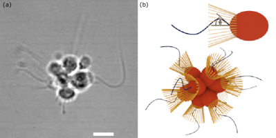
Figure 1: (color online) The choanoflagellate S. rosetta. (a) Bright field image ($5$ $\mu$m scale) and (b) schematics of ‘slow-swimmer’ single cell, base angle $\theta$, and rosette colony.

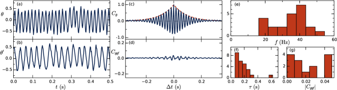
Figure 2: (color online) Flagellar beating dynamics. (a,b) Time series of the base angle $\theta(t)$ on two flagella within a single colony. (c) Autocorrelation function of $\theta$ for one flagellum, with fit of the envelope to an exponential decay (dashed red). (d) Cross correlation of $\theta$ between two flagella on the same colony. (e) Peak frequencies of $n=23$ tracked flagella. (f) Decay time of autocorrelation in single flagella. (g) Magnitude of cross correlations between flagella in same colonies.

S. rosetta (obtained from Dr. Barry Leadbeater, University of Birmingham, UK) were cultured in artificial seawater ($36.5$ g/L Marin Salts (Tropic Marin, Germany)). To provide a food source for prey bacteria, organic enrichment ($4$ g/L Proteose Peptone (Sigma-Aldrich, USA), $0.8$ g/L Yeast Extract (Fluka Biochemika)) was added to the cultures at $15$ $\mu$l/ml. Cultures were grown at 22^∘C and split every $4-7$ days. To study the flagella beat dynamics, colonies were stuck to poly-L-lysine (0.01%, Sigma) treated microscope slides and flagella beats imaged at 500 fps (Fastcam SA3, Photron, USA) in bright field. Image template matching was employed to track the motion of the only slightly moving colonies, and in the local frame of the organism, the bases of the flagella were tracked by techniques similar to that of the active contour model Kass1988 , yielding as a readout of beating the angle $\theta(t)$ defined in Fig. 1b.

Figs. 2a,b show $\theta(t)$ from two flagella on the same colony, and it is clear that they have distinct frequencies. In general, the beating frequencies $f$, found by Fourier transforming $\theta(t)$, show a surprisingly high variability (Fig. 2e). The normalized autocorrelation $C_{\theta}(\Delta t)=\langle\theta(t)\theta(t+\Delta t)\rangle_{t}/\langle\theta(t)^{2}\rangle_{t}$ for a single flagellum is plotted in Fig. 2c. Similar to the function discussed Ma2014 ; Wan2014 in the context of flagellar beating in Chlamydomonas, the data are consistent with $C_{\theta}=\exp(-|t|/\tau)\cos(2\pi f\,t)$, the envelope of which is shown in the figure. The decay time $\tau$ also shows a very high degree of variability (Fig. 2f), but all are $<1$ s suggesting high stochasticity. Within colonies, the cross correlation between flagella $C_{\theta,\theta^{\prime}}(\Delta t)=\langle\theta(t)\theta^{\prime}(t+\Delta t)\rangle_{t}/\sqrt{\langle\theta(t)^{2}\rangle_{t}\langle\theta^{\prime}(t)^{2}\rangle_{t}}$ (Fig. 2d) is negligible (only a very slight signal can be made out, which we attribute to the overall wiggling of the colony – see Supplemental Video 1). All cross-correlation signals were found to be less than $0.05$ (Fig. 2g). The lack of correlation between beating flagella in colonies makes S. rosetta an ideal model organism for ARWs.

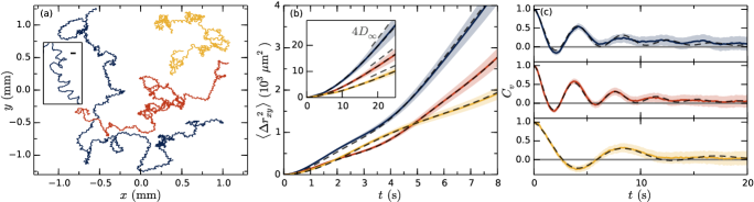
Figure 3: (colour online) Random walks. (a) Long tracks of swimming S. rosetta. Inset scale bar is $10$ $\mu$m. (b) Projected mean squared displacement for individual walks (solid, error shaded) and fits of model (dashed). Inset shows a zoom-out with late-time linear behavior $\sim 4D_{\infty}t$ (dashed, gray). (c) Velocity autocorrelation (solid, error shaded) and model (dashed) with parameters as in (b). Fitted parameters (red curve): $\omega_{0}=1.63$ s^-1, $v_{p}=8.45$ $\mu$m/s, $v_{\omega}=12.7$ $\mu$m/s, $D_{r}=0.10$ s^-1.

In studying the swimming trajectories of S. rosetta, ensemble averages taken over many colonies will eliminate features related to colony-specific morphology (cell location and flagella orientation). To overcome this lack of ‘ergodicity’, we obtained long tracks of $36$ individual colonies. In-house software logged and synchronized the position of the $xy$-stage (MS-2000, ASI, USA) to a camera (Imaging Source, Germany) filming in bright field at $15$ fps. This enabled tracking of colonies moving in three dimensions at distances much longer than the field of view. To track the particles a Gaussian-mixture model KaewTraKulPong2002 was applied to estimate the moving background and subsequently the tracks were manually controlled. Fig. 3a shows three examples, all $\sim 20$ minutes in length. On close inspection (inset of Fig. 3a) we observe that the trajectories are noisy helices. The mean squared displacement $\langle\Delta r_{xy}^{2}\rangle=\langle[\textbf{x}_{xy}(s+t)-\textbf{x}_{xy}(s)]^{2}\rangle_{s}$ (Fig. 3b), shows an early time ballistic $\sim t^{2}$ behavior (for $t<1$ s) and late time diffusive $\sim t$ form (inset) similar to that of Janus particles Howse2007 . However, comparing these curves to those of conventional active Brownian particles (see SI), we observe a different intermediate time behavior. These bumps (Fig. 3b) appear precisely because some of the constituent cells may beat off center and induce internal (effective) torques producing stochastic helical trajectories. To highlight the underlying regularity of this helical swimming, we calculate the velocity autocorrelation $C_{v}(t)=\langle\textbf{v}_{xy}(s+t)\cdot\textbf{v}_{xy}(s)\rangle_{s}$ (Fig. 3c) which oscillates at the frequency of the induced rotation and decays on a timescale of several oscillation periods.

Active random walks have been the attention of much research Lovely1974 ; Lauga2011 , but only recently have rotational torques been incorporated. External torques appear on e.g. magnetotactic bacteria in the presence magnetic fields Blakemore1980 and gyrotactic organisms such as certain algae in gravitational fields Pedley1990 and can be treated analytically Sandoval2013 . However, the present internal torques can be treated analytically only in 2D VanTeeffelen2008 and numerical Wittkowski2012 or approximative Friedrich2009 methods are needed in 3D. Below we develop an approximate 3D theory with the goal of simple analytical functions that can be used to extract physical quantities and interpret the data.

The diffusion of a random walker can be described by the Langevin equation $\mathrm{d}{\boldsymbol{x}}(t)={\boldsymbol{v}}(t)\,\mathrm{d}t+\sqrt{2D}\,\mathrm{d}{\boldsymbol{W}}(t)$, where $D$ is the translational diffusion constant and ${\boldsymbol{W}}(t)$ a standard vector Wiener process with $\langle\mathrm{d}{\boldsymbol{W}}_{i}(t)\,\mathrm{d}{\boldsymbol{W}}_{j}(t^{\prime})\rangle=\delta_{ij}\delta(t-t^{\prime})$. The case ${\boldsymbol{v}}(t)={\bf 0}$ is a passive particle and leads to the projected mean squared displacement $\langle\Delta r_{xy}^{2}\rangle\equiv\langle\Delta x^{2}+\Delta y^{2}\rangle=4\,Dt$. Building an ARW from passive particles leads to no new behavior, but motile particles also have a stochastic velocity term. In the simplest case in two dimensions, the speed $v$ is constant and ${\boldsymbol{v}}(t)=v\left(\cos\theta(t),\sin\theta(t)\right)$ evolves stochastically through $\theta(t)$. The choice $\mathrm{d}\theta=\sqrt{2D_{r}}\,\mathrm{d}W_{r}(t)$ leads to the conventional result $\langle\Delta r_{xy}^{2}\rangle=(2v^{2}/D_{r}^{2})\left(D_{r}t+e^{-D_{r}t}-1\right)+4\,Dt$, which behaves ballistically, $\langle\Delta r^{2}\rangle\sim t^{2}$, at early times, but diffusively, $\langle\Delta r^{2}\rangle\sim t$, at longer times (see SI) with an enhanced diffusion constant $D_{\infty}=D+v^{2}/2D_{r}$, describing well the motion of Janus particles Howse2007 . This is a 2D result. Contrary to passive random walkers, active random walkers’ effective diffusion constant can vary with dimension. The corresponding 3D result is $D_{\infty}=D+v^{2}/3D_{r}$ given a similar definition of 3D rotational diffusion. Typically, $D\ll v^{2}/D_{r}$ and passive diffusion can be ignored.

The Reynolds number for S. rosetta is $\text{Re}\sim 10^{-4}$. At such low Reynolds numbers, inertia is negligible and the fluid dynamics becomes governed by the linear Stokes equation. Accordingly, self-propelled choanoflagellates are both force- and torque-free. We assume that S. rosetta are sphere-like such that couplings between translations and rotations can be ignored. Heuristically, the velocity of a colony ${\boldsymbol{v}}(t)$ is approximately a linear sum of the velocities that the constituents would have had swimming independently, ${\boldsymbol{v}}(t)\approx\eta\sum{\boldsymbol{v}}_{i}(t)$, the factor $\eta$ accounting for the change in drag with the radius $a$ of the colony, as $\eta\sim a^{-1}$. If some of the walkers comprising the colony, placed at positions $\{{\bf r}_{i}\}$, beat off center, an angular velocity ${\boldsymbol{\omega}}(t)\approx\eta_{r}\sum{\boldsymbol{r}}_{i}\times{\boldsymbol{v}}_{i}$ will also be induced, where $\eta_{r}\sim a^{-3}$. Since $\{{\boldsymbol{v}}_{i}\}$ and $\{{\boldsymbol{r}}_{i}\}$ are given in the local coordinate system of the particle, they must be rotated along with the particle. For a two dimensional ARW, this motion is described by ${\boldsymbol{v}}(t)=v(t)\left(\cos\theta(t),\sin\theta(t)\right)$, where $v(t)=|{\boldsymbol{v}}(t)|$, $\mathrm{d}\theta=\omega(t)\,\mathrm{d}t+\sqrt{2D_{r}}\,\mathrm{d}W(t)$, $\omega(t)=\pm|{\boldsymbol{\omega}}(t)|$, and $D_{r}$ is an effective rotational diffusion constant which can be calculated if the individual stochastic processes are prescribed. With $v(t)$ constant, constant $\omega(t)$ yields circles in the absence of noise. In three dimensions, such motion leads to helices, making (2D-projected) three dimensional ARWs behave very differently from 2D ones and necessitating a full 3D theory.

With the goal of a minimal model, we take the swimming speed to be constant and let the direction of the velocity evolve with the rotation of the organism according to $\mathrm{d}{\boldsymbol{v}}(t)=\mathrm{d}{\boldsymbol{\Omega}}(t)\times{\boldsymbol{v}}(t)$, where $\mathrm{d}{\boldsymbol{\Omega}}(t)={\boldsymbol{\omega}}(t)\,\mathrm{d}t+\sqrt{2D_{r}}\,{\boldsymbol{\Lambda}}(t)\,\mathrm{d}W_{r}(t)$. Here, ${\boldsymbol{\Lambda}}(t)$ is a random unit vector orthogonal to ${\boldsymbol{v}}(t)$, uncorrelated in time. To limit further the number of model parameters we assume the magnitude of ${\boldsymbol{\omega}}(t)$ is constant, while its direction obeys $\mathrm{d}{\boldsymbol{\omega}}(t)=\sqrt{2D_{r}}\,{\boldsymbol{\Lambda}}(t)\times{\boldsymbol{\omega}}(t)\,\mathrm{d}W_{r}(t)$. This last update makes the system analytically quite intractable and thus we shall seek an approximate solution. As motivation, consider the case $D_{r}=0$ with specified initial conditions ${\boldsymbol{v}}(0)={\boldsymbol{v}}_{0}$, ${\boldsymbol{\omega}}(0)={\boldsymbol{\omega}}_{0}$. This system can be solved exactly to yield ${\boldsymbol{x}}(t)={\boldsymbol{x}}_{0}+[(\omega_{0}({\boldsymbol{\omega}}_{0}\cdot{\boldsymbol{v}}_{0}){\boldsymbol{\omega}}_{0}t+{\boldsymbol{\omega}}_{0}\times({\boldsymbol{v}}_{0}\times{\boldsymbol{\omega}}_{0})\sin(\omega_{0}t)+\omega_{0}({\boldsymbol{\omega}}_{0}\times{\boldsymbol{v}}_{0})(1-\cos(\omega_{0}t))]/\omega_{0}^{3}$, or

$${\boldsymbol{x}}(t)=\int_{0}^{t}{\boldsymbol{v}}(t^{\prime})\,\mathrm{d}t^{\prime}, {\boldsymbol{v}}(t)={\boldsymbol{R}}\cdot\begin{pmatrix}v_{\omega}\cos\omega_{0}t\\ v_{\omega}\sin\omega_{0}t\\ v_{p}\end{pmatrix},$$ (1)

where $v_{\omega}=|{\boldsymbol{\omega}}_{0}\times{\boldsymbol{v}}_{0}|/\omega_{0}$, $v_{p}={\boldsymbol{\omega}}_{0}\cdot{\boldsymbol{v}}_{0}/\omega_{0}$, $\omega_{0}=|{\boldsymbol{\omega}}_{0}|$, and ${\boldsymbol{R}}$ is some orthogonal matrix. Eq. (1) describes a helix of radius $v_{\omega}/\omega_{0}$ and mean speed $v_{p}$ (averaged over $2\pi/\omega_{0}$). The form of (1) inspires an approximative solution in the presence of noise in which the deterministic helix parameters define a continuous-time random walk with helix-like steps, the matrix ${\boldsymbol{R}}$ becoming a stochastic matrix process. As an effective description we assume ${\boldsymbol{R}}(t)={\boldsymbol{R}}_{x}(\alpha)\cdot{\boldsymbol{R}}_{y}(\beta)\cdot{\boldsymbol{R}}_{z}(\gamma)$, where the matrix factors are rotations around the $x,y,z$ axes. $\alpha,\beta,\gamma$ are taken independent and identically distributed with $\mathrm{d}\alpha=\sqrt{2D_{r}}\,\mathrm{d}W_{\alpha}(t)$. This approximation makes the system much more manageable. While the approach breaks $x-y$ symmetry, simulations show it to be an overall good approximation for the statistics of interest

In the stationary limit we find (see SI):

$$\langle{\boldsymbol{v}}_{xy}(\Delta t)\cdot{\boldsymbol{v}}_{xy}(0)\rangle =\frac{e^{-2D_{r}|\Delta t|}}{8}\Big{[}2v_{p}^{2}\left(1+2e^{D_{r}|\Delta t|}\right)$$ (2)

$$+v_{\omega}^{2}\left(4+e^{-D_{r}|\Delta t|}\right)\cos(\omega_{0}\Delta t)\Big{]}.$$

The $xy$-projected mean squared displacement becomes

$$\langle\Delta r^{2}_{xy}\rangle=\frac{v_{p}^{2}e^{-D_{r}t}}{D_{r}^{2}}\Big{(}1+\frac{e^{-D_{r}t}}{8}\Big{)}+4D_{\infty}t-a_{0}$$ (3)

$$+v_{\omega}^{2}e^{-2D_{r}t}\Big{(}\frac{4D_{r}^{2}-\omega_{0}^{2}}{(4D_{r}^{2}+\omega_{0}^{2})^{2}}+\frac{(9D_{r}^{2}-\omega_{0}^{2})e^{-D_{r}t}}{4(9D_{r}^{2}+\omega_{0}^{2})^{2}}\Big{)}\cos\omega_{0}t$$

$$-v_{\omega}^{2}e^{-2D_{r}t}\Big{(}\frac{4\omega_{0}D_{r}}{(4D_{r}^{2}+\omega_{0}^{2})^{2}}+\frac{3\omega_{0}D_{r}e^{-D_{r}t}}{2(9D_{r}^{2}+\omega_{0}^{2})^{2}}\Big{)}\sin\omega_{0}t,$$

where the constant $a_{0}$ enforces $\langle\Delta r^{2}_{xy}\rangle(t=0)=0$. As $t\to\infty$ we obtain $\langle\Delta r^{2}_{xy}\rangle=4D_{\infty}t$, where

$$D_{\infty}=\frac{5v_{p}^{2}}{16D_{r}}+\frac{v_{\omega}^{2}D_{r}}{8}\left(\frac{1}{6D_{r}^{2}+\frac{2}{3}\omega_{0}^{2}}+\frac{1}{D_{r}^{2}+\frac{1}{4}\omega_{0}^{2}}\right).$$ (4)

These results have been verified by simulations using the Euler-Maruyama method. It has previously been shown that reciprocal swimming enhances diffusion Lauga2011 , and the last terms of (13), which are major contributions to the diffusion constant, embody this phenomenon.

Equations (10) and (11) describe the approximate functions corresponding to the data of Figs. 3c and 3b, respectively. The diffusion constant $D_{\infty}$ can be extracted from the linear late-time behavior of $\langle\Delta r^{2}_{xy}\rangle$ (dashed gray in inset of Fig. 3b), and can be used in (13) to fix one of the model parameters in terms of the others. The remaining three are fitted simultaneously to the curves of Fig. 3b and 3c. The experimental data are well-described by the model as shown by the dashed lines in the figures. The relative magnitudes of the extracted velocities, $v_{p}$ and $v_{\omega}$, reveal how much energy the organisms spent on effective ($v_{p}$) and circular ($v_{\omega}$) swimming, for example the blue curve in Fig. 3 has $v_{p}=10.6$ $\mu$m/s and $v_{\omega}=14.2$ $\mu$m/s. While not producing the precise morphologies of the colonies, the fitted velocities combined with the extracted frequency $\omega_{0}$, do constrain the possible configurations. Using the fitted velocities and a colony radius $a\sim 5$ $\mu$m, we find an effective translational force of $\sim 1$ pN, and using $\omega_{0}$, an effective torque $\sim 4$ pN$\cdot$ $\!\mu$m: the small residual forces that propel and rotate a colony are on the order of that of a single cell.

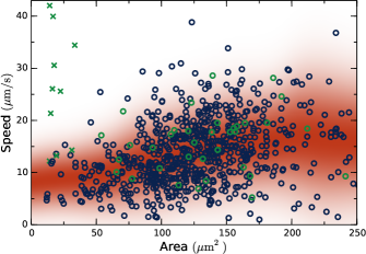
Figure 4: (colour online) Speed versus size for $\sim 750$ colonies. Colony size is estimated by median $xy$-projected area. Colonies are blue and green circles, green speed being $\sqrt{v_{p}^{2}+v_{\omega}^{2}}$ from model fits to the long tracks. Green crosses are single-celled fast swimmers Dayel2011 . Colored background indicates running mean and standard deviation.

Just as flagella beating in S. rosetta varies between cells, morphology varies between colonies as a result of the cell division process Fairclough . This stochasticity enables two colonies of similar size to swim very differently. To quantify this, we used in-house software to track $\sim 750$ colonies of varying size swimming in quasi-2D between two cover slips, and when a colony was in focus the area of an ellipse fitted to its outline served as an estimator of size (see Supplemental Video 2). This method, while introducing uncertainty in area, enables high throughput. To obtain model parameters, long tracks are needed. The parameters for 36 such tracks are given in the SI, and the speed $\sqrt{v_{p}^{2}+v_{\omega}^{2}}$ of those tracks is shown in Fig. 4 as green circles. There is a slow increase in speed with colony size. This trend can be explained by simple ad-hoc models such as random orientation of cells in a sphere-like structure: drag scales linearly with radius $a$ but maximum propulsive force (the case where all propulsive forces point in one direction) scales like $a^{2}$. However, there is an intriguing lack of very slow swimmers which would be predicted by such a model. Indeed giving cells an orientation more parallel with its location would only yield slower swimming speeds. More importantly, Fig. 4 shows just how different colonies of similar size are: the stochastic processes underlying colony formation have high variances. From fits of the long tracks this stochasticity seems to apply to all model parameters (SI). This is contrary to e.g. bacterial clumps where rotation rate clearly decreases with size Poon . Contrary to the phototactic response of Chlamydomonas and Volvox in which the time-scale of rotation is matched to inner chemistry Drescher2010 , or the chemotactic response of sperm cells in which curvature and torsion of swimming paths are directly manipulated by the single beating flagellum Friedrich2009 , due to this stochastic morphology of S. rosetta, knowledge of the overall colony morphology and motion (e.g. $\omega_{0}$) is arguably not available at the single-cell level, rendering ‘deterministic’ chemotactic strategies difficult. Thus one of the most important issues is the possibility of chemotaxis in aggregate random walks through suitable modulation of the independent constituents preprint .

A fundamental operation in the theory of stochastic processes is their summation to yield a single effective process. The corresponding operation for random walkers, ‘stitching’ them together, yields ARWs. As we have shown, there is a crucial complexity for random walkers: the underlying flagellar beating can also yield rotations, so the ‘summation rules’ differ. Our results suggest that for simple random walkers the ARWs can be described approximately through four numbers: $v_{\omega}$, $v_{p}$, $\omega_{0}$, and $D_{r}$. The question of the correct ‘summation rules’ for general random walkers (e.g. anisotropic, hydrodynamically translation-rotation coupled, or non-identical constituents) remains open. Likewise, the transition, via e.g. self-assembly or flagella growth, from high to low stochasticity in ARWs with non-independent constituents is intriguing. The present exemplar, S. rosetta, is a very good approximation to what one might call an ideal biological ARW: independent constituents and a roughly spherical shape. Its mode of swimming raises many interesting questions about the evolution of multicellularity and on the nature and origin of noise, both internal and environmental.

Supplemental Information

Motility of Colonial Choanoflagellates and the Statistics of Aggregate Random Walkers

Julius B. Kirkegaard, Alan O. Marron, Raymond E. Goldstein

Single cells

Slow-swimmer S. rosetta unicells, similar in morphology to the individual cells that comprise a colony, clearly exhibit random walk behaviour. Fig. 5 shows the average square displacement of 32 S. rosetta slow-swimmers each filmed for $\sim$1.5 minutes. The behaviour is well-described by the equation for conventional active random walkers,

$$\langle\Delta r_{xy}^{2}\rangle=(2v^{2}/D_{r}^{2})\left(D_{r}t+e^{-D_{r}t}-1\right).$$ (5)

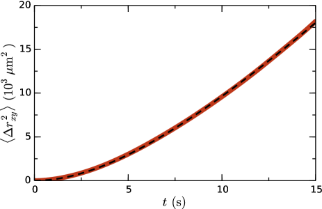
Figure 5: Squared distance moved averaged over 32 S. rosetta single cells. Overlayed fit in dashed is to Eq. (5). Parameters: $v=12.3$ $\mu$m/s, $D_{r}=0.15$ s^-1.

The active rotational diffusion constant for both single cells and colonies (main text) are on the order of $0.1$ $s^{-1}$. With a beat frequency of $\sim 40$ Hz this corresponds to a $\sim 3^{\circ}$ rotational deviation per beat. The thermal rotational diffusion constant $D_{r}^{\text{thermal}}=k_{B}T/8\pi\mu a^{3}$ ranges from $0.012$ to $0.0014$ $s^{-1}$ for radii $2.5$ to $5.0$ $\mu$m, at least an order magnitude below the active one.

Derivation of random walker functions

Since $\alpha$, $\beta$, and $\gamma$ are Markov processes we can write e.g. $P(\alpha(t^{\prime}))=N(\alpha_{0},\penalty 02D_{r}\,t^{\prime})$ and $P(\alpha(t)|\alpha(t^{\prime}))=N(\alpha(t^{\prime}),\penalty 02D_{r}\,(t-t^{\prime}))$ for $t^{\prime}<t$, where $N(\mu,\sigma^{2})$ is the normal distribution. Using $P(\alpha(t),\alpha(t^{\prime}))\penalty 0=P(\alpha(t)|\alpha(t^{\prime}))\penalty 0P(\alpha(t^{\prime}))$ we obtain averages such as

$$\langle\cos\alpha(t)\cos\alpha(t^{\prime})\rangle=\int_{-\infty}^{\infty} \mathrm{d}x\int_{-\infty}^{\infty}\mathrm{d}y\cos(x)\cos(y)$$ (6)

$$\times N_{x}(\alpha_{0},2D_{r}\min(t,t^{\prime})|)N_{y}(x,2D_{r}|t-t^{\prime}|)$$

$$=\frac{1}{2}e^{-D_{r}|t-t^{\prime}|}\big{(}1+\cos(2\alpha_{0})e^{-4D_{r}\text{min}(t,t^{\prime})}\,\big{)},$$

which in the stationary limit can be used to find the velocity autocorrelations, e.g.

$$\langle v_{x}(t)v_{x}(s)\rangle =\Big{\langle}\big{(}v_{\omega}\cos(\beta(t))\cos(\gamma(t))\cos(\omega_{0}t)+v_{p}\sin(\beta(t))$$ (7)

$$\quad-v_{\omega}\cos(\beta(t))\sin(\gamma(t))\sin(\omega_{0}t)\big{)}\times\big{(}v_{p}\sin(\beta(s))$$

$$\quad+v_{\omega}\cos(\beta(s))\cos(\gamma(s))\cos(\omega_{0}s)-v_{\omega}\cos(\beta(s))\sin(\gamma(s))\sin(\omega_{0}s)\big{)}\Big{\rangle}$$

$$=\frac{1}{2}\,v_{p}^{2}\,e^{-D_{r}|t-s|}+\frac{1}{4}\,v_{\omega}^{2}e^{-2D_{r}|t-s|}\,\cos(\omega_{0}(t-s)).$$

The function only depends on the time difference $t-s$, which is the case for stationary autocorrelations (this is the very definition of a weakly stationary process). From

$$v_{y}(t) =-v_{p}\sin(\alpha(t))\cos(\beta(t))+v_{w}\big{(}\big{[}\sin(\alpha(t))\sin(\beta(t))\cos(\gamma(t))$$ (8)

$$\quad+\cos(\alpha(t))\sin(\gamma(t))\big{]}\cos(\omega_{0}t)+\big{[}\cos(\alpha(t))\cos(\gamma(t))$$

$$\quad-\sin(\alpha(t))\sin(\beta(t))\sin(\gamma(t))\big{]}\sin(\omega_{0}t)\big{)}$$

we find in a similar manner

$$\langle v_{y}(t)v_{y}(s)\rangle=\frac{1}{4}\,v_{p}^{2}\,e^{-2D_{r}|t-s|}+\frac{1}{8}\,v_{\omega}^{2}\big{(}e^{-3D_{r}|t-s|}+2e^{-2D_{r}|t-s|}\big{)}\,\cos(\omega_{0}(t-s)).$$ (9)

Thus

$$\langle{\boldsymbol{v}}_{xy}(\Delta t)\cdot{\boldsymbol{v}}_{xy}(0)\rangle =\frac{e^{-2D_{r}|\Delta t|}}{8}\Big{[}2v_{p}^{2}\left(1+2e^{D_{r}|\Delta t|}\right)+v_{\omega}^{2}\left(4+e^{-D_{r}|\Delta t|}\right)\cos(\omega_{0}\Delta t)\Big{]}.$$ (10)

The $xy$-projected mean squared displacement is obtained by integrating the autocorrelation twice

$$\langle\Delta r^{2}_{xy}\rangle =\int_{0}^{t}\int_{0}^{t}\langle{\boldsymbol{v}}_{xy}(t^{\prime})\cdot{\boldsymbol{v}}_{xy}(t^{\prime\prime})\rangle\,\mathrm{d}t^{\prime}\mathrm{d}t^{\prime\prime}$$ (11)

$$=\frac{v_{p}^{2}e^{-D_{r}t}}{D_{r}^{2}}\Big{(}1+\frac{e^{-D_{r}t}}{8}\Big{)}+4D_{\infty}t-a_{0}$$

$$\quad+v_{\omega}^{2}e^{-2D_{r}t}\Big{(}\frac{4D_{r}^{2}-\omega_{0}^{2}}{(4D_{r}^{2}+\omega_{0}^{2})^{2}}+\frac{9D_{r}^{2}-\omega_{0}^{2}}{4(9D_{r}^{2}+\omega_{0}^{2})^{2}}e^{-D_{r}t}\Big{)}\cos\omega_{0}t$$

$$\quad-v_{\omega}^{2}e^{-2D_{r}t}\Big{(}\frac{4\omega_{0}D_{r}}{(4D_{r}^{2}+\omega_{0}^{2})^{2}}+\frac{3\omega_{0}D_{r}}{2(9D_{r}^{2}+\omega_{0}^{2})^{2}}e^{-D_{r}t}\Big{)}\sin\omega_{0}t,$$

where

$$a_{0}=\frac{9v_{p}^{2}}{8D_{r}^{2}}+{\boldsymbol{v}}_{\omega}^{2}\left(\frac{4D_{r}^{2}-\omega_{0}^{2}}{(4D_{r}^{2}+\omega_{0}^{2})^{2}}+\frac{9D_{r}^{2}-\omega_{0}^{2}}{4(9D_{r}^{2}+\omega_{0}^{2})^{2}}\right).$$ (12)

As $t\to\infty$, $\langle\Delta r^{2}_{xy}\rangle\sim 4D_{\infty}t$, where

$$D_{\infty}=\lim_{t\rightarrow\infty}\frac{\langle\Delta r^{2}_{xy}\rangle}{4t}=\frac{5v_{p}^{2}}{16D_{r}}+\frac{v_{\omega}^{2}D_{r}}{8}\left(\frac{1}{6D_{r}^{2}+\frac{2}{3}\omega_{0}^{2}}+\frac{1}{D_{r}^{2}+\frac{1}{4}\omega_{0}^{2}}\right).$$ (13)

The existence of the above (non-zero) limit confirms the diffusive behaviour.

Comparison of fit parameters

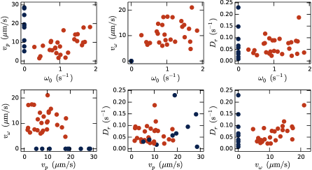
Figure 6: Comparison of fit parameters of 36 tracks. Tracks where $\omega_{0},v_{\omega}$ could be determined in red and tracks where $\omega_{0},v_{\omega}$ are forced to zero in blue.

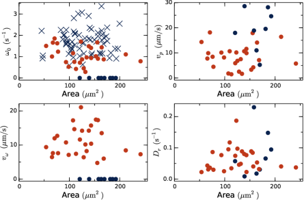
Figure 7: Comparison of fit parameters of 36 tracks to size of colony. Tracks where $\omega_{0},v_{\omega}$ could be determined in red and tracks where $\omega_{0},v_{\omega}$ are forced to zero in blue. $\omega_{0}$ plot additionally includes estimates from the short track data in blue crosses.

Fig. 6 shows scatter plots of fit parameters of the model to 36 different S. rosetta colonies, indicating the high variances of all parameters. We note, however, that the determination of some parameters are difficult in certain regions. For instance, $\omega_{0}$ and $v_{\omega}$ are hard to determine when either one becomes small, and accordingly we have forced them to zero in these cases and plotted them in blue. Naturally, these cases will have a higher $v_{p}$ as is clear in the two plots in the left part of Fig. 6.

Applying the same area estimator as in Fig. 4 of the main text, the parameters can also be plotted as a function of size. Just as with swimming speed, Fig. 7 shows that the model parameters have very high variances and no clear dependency on size. For a subset of the short tracks we were able to fit the model well enough to estimate $\omega_{0}$ and these are shown as blue crosses. However, the short track colonies for which good estimated could be obtained are biased towards high $\omega_{0}$ (and $v_{\omega}$). Nonetheless, there is no clear tendency for larger colonies to rotate slower as is the case for e.g. bacterial clumps PoonSI . For an interesting example of a big fast-spinning colony see end of Supplemental Video 2 in which a colony has formed as a dumb-bell shape.

References

- (1) J. Schwarz-Linek, C. Valeriani, A. Cacciuto, M.E. Cates, D. Marenduzzo, A.N. Morozov, and W.C.K. Poon, Phase separation and rotor self-assembly in active particle suspensions, Proc. Natl. Acad. Sci. USA 109, 4052-4057 (2012).