Time-evolution of holographic entanglement entropy
and metric perturbations

Abstract

We study the holographic entanglement entropy under small deformations of AdS, including time-dependence. It is found through perturbative analysis that the divergent terms are not affected and the change appears only in the finite terms. We also consider the entanglement thermodynamic first law, and calculate the entanglement temperature and confirm that it is inversely proportional to the size of the entangling region.

I Introduction

The holographic principle Hooft:1993gx ; Susskind:1994vu ; Maldacena:1997re relates a certain strongly-coupled field theory to a quantum gravity system in one higher dimensions. It is an intriguing proposal, when we note the possibility of spacetime emerging naturally from a quantum system without gravitational degrees of freedom per se. The holographic entanglement entropy (HEE) prescription Ryu:2006bv provides a versatile tool in this line of study, since unlike other probes like Wilson loops which are dual to fundamental strings, it involves model-independent and universal concepts like quantum entanglement and volume-minimizing submanifold etc.

Another valuable insight into this relation is motivated by the so-called AdS/MERA correspondence Swingle:2009bg . MERA, or multi-scale entanglement renormalization ansatz, is a particular version of tensor network method in the study of critical lattice system Vidal:2007hda . In MERA, one considers the real-space renormalized lattice system together with the original lattice system and extremizes the energy of the entire system, from UV to IR. In this picture a holographic direction in AdS/CFT language is incorporated by construction, and one can argue that the metric in the entire space is the hyperbolic space, which is just the constant time slice of AdS. It is certainly of great interest to promote such observations to full-fledged time-dependent backgrounds. Namely, we hope to be able to see propagating gravitons constructed out of time-dependent process in a strongly-coupled quantum system. The present work is a modest step towards that goal and we will study the time-evolution of HEE in time-dependent backgrounds.

The Ryu-Takayanagi proposal has been generalized to covariant formulae to suit generic backgrounds in Hubeny:2007xt , and in this paper we will study the behavior of extremal codimension-two surfaces in backgrounds which are small deformations of pure AdS spacetime. There exist works which studied the evolution of HEE in time-dependent setups already, but as far as we know they mostly use a rather special class of metric called AdS-Vaidya solutions, or make use of numerically constructed solutions Balasubramanian:2010ce ; Balasubramanian:2011ur ; Balasubramanian:2011at ; Allais:2011ys ; Keranen:2011xs ; Caceres:2012em ; Baron:2012fv ; Hubeny:2013hz ; Liu:2013iza ; Liu:2013qca ; Hubeny:2013dea ; Alishahiha:2014jxa ; Bai:2014tla ; daSilva:2014zva ; Ugajin:2014nca ; Keranen:2015fqa ; Ziogas:2015aja . Conceptually our study is more similar to papers such as Leichenauer:2015nxa ; Mishra:2015cpa which adopted a perturbative approach, but we are interested in time-dependendent backgrounds.

In Sec.2 we start by computing the HEE for cap-like regions in global coordinate of AdS, and sketch how HEE can be computed perturbatively in backgrounds with time-dependence. For simplicity we restrict ourselves to spherically-symmetric backgrounds. In Sec.3 we apply the method to AdS-Schwarzschild black holes and also to the time-periodic solutions of AdS-scalar field system constructed in Maliborski:2013jca ; Kim:2014ida . One generic feature we obtained is that the effect of metric perturbation on HEE starts with the finite part, and there is no change in the leading-order or logarithmically divergent terms. In Sec.4 we use our results to compute the holographic entanglement temperature and verify that it is inversely proportional to the size of the entangling region, with a universal coefficient. We conclude with a couple of comments in Sec.5.

II HEE with metric perturbations

II.1 HEE in pure AdS

As a warm-up and also to set up the notation let us consider the holographic entanglement entropy of pure AdS in generic dimensions. The metric convention we take for $AdS_{d+1}$ spacetime with radius $\ell$ is

$$ds^{2}=\frac{\ell^{2}}{\cos^{2}x}(-dt^{2}+dx^{2}+\sin^{2}x(d\theta^{2}+\sin^{2}\theta d\Omega_{d-2}^{2})),$$ (1)

where for later convenience we split the $S^{d-1}$ metric into polar angle $\theta$ and unit-radius sphere $S^{d-2}$ with metric $d\Omega_{d-2}^{2}$.

In this paper we choose the entangling region on the boundary to be a cap-like one defined by $0\leq\theta<\theta_{0}$ and at boundary time $t=t_{0}$. The holographic entanglement entropy (HEE) is then the extremized area from the following functional of $x(\theta)$,

$$\text{Area}=\ell^{d-1}\text{vol}(S^{d-2})\int^{\theta_{0}}_{0}d\theta\frac{(\sin x\sin\theta)^{d-2}}{\cos^{d-1}x}\sqrt{\left(\frac{dx}{d\theta}\right)^{2}+\sin^{2}x}\,\,.$$ (2)

Without losing generality we assume $\theta_{0}<\pi/2$. The most general form of the solution derived from the action (2) is difficult to find, but one can check the following function satisfies the Euler-Lagrange equation from (2) for any $d$ Bakas:2015opa :

$$x(\theta)=\sin^{-1}\left(\frac{a}{\cos\theta}\right).$$ (3)

This solution is related through a conformal transformation to the hemisphere solutions of a spherical-shape entangling surface in Poincaré coordinates. We may call them constant-latitude solutions because $\sin x\cos\theta=a$. Since the boundary is at $x=\pi/2$, we have $a=\cos\theta_{0}$. These curves are plotted in Fig.1(a), using $x$ as the radial coordinate.

We will consider small deformations of $AdS$ background and see how the minimal area solutions (3) changes accordingly. Instead of the original parametrization, we find that it is more advantageous to use the following variables.

$$z:=\cos\theta,\quad\rho:=\sin x\,.$$ (4)

Then the area functional becomes

$$\text{Area}=\ell^{d-1}\text{vol}(S^{d-2})\int^{1}_{\cos^{-1}\theta_{0}}dz\frac{\rho^{d-2}(1-z^{2})^{(d-2)/2}}{(1-\rho^{2})^{d/2}}\sqrt{(\rho^{\prime})^{2}+\frac{\rho^{2}(1-\rho^{2})}{1-z^{2}}}.$$ (5)

To calculate HEE we need to substitute the solution $\rho=a/z$ back into (5), and perform the integral. As it is usually the case with AdS/CFT, the integral is divergent near the boundary $x=\pi/2$ and a regularization process is required. We introduce a cutoff at $x_{m}=\pi/2-\epsilon$. When applied to the reference solution (3),

$$\theta_{m}=\theta_{0}-\frac{1}{2}\epsilon^{2}\cot\theta_{0},\quad\text{i.e.}\quad z_{m}=a\left(1+\frac{\epsilon^{2}}{2}\right).$$ (6)

We list the result of regularized HEE for spherical entangling surface in various dimensions as a series expansion in $\epsilon$ in Table. 1. The result for pure AdS corresponds to $M=0$ cases in Table 1, and $M\neq 0$ cases will be discussed in Sec.III.1. As it is well known the leading-order divergent terms exhibit the area law. When the boundary theory is even-dimensional, i.e. $d$ is even it also contains logarithmic divergence, whose coefficient is universal and related to the central charge Takayanagi:2012kg ; Nishioka:2009un ; Ryu:2006bv .

	$\text{Area}/(\ell^{d-1}\text{vol}(S^{d-2}))$
$AdS_{3}$	$2\log\left(\frac{1}{\epsilon}\right)+2\log(2\sin\theta_{0})+\cdots.$
$AdS_{4}$	$\sin\theta_{0}\left(\frac{1}{\epsilon}\right)-1+M\frac{\csc\theta_{0}(1-3\cos\theta_{0}+\cos 2\theta_{0}+\sec\theta_{0})}{3}+\cdots.$
$AdS_{5}$	$\frac{\sin^{2}\theta_{0}}{2}\left(\frac{1}{\epsilon}\right)^{2}-\frac{1}{2}\log\left(\frac{1}{\epsilon}\right)-\frac{\cos 2\theta_{0}}{12}-\frac{1+3\log 2}{6}-\frac{\log(\sin\theta_{0})}{2}$
	$+M\frac{\csc^{2}\theta_{0}(3+3\cos\theta_{0}+6\cos^{4}\theta_{0}+3\theta\sec\theta_{0}\sin 3\theta_{0})}{16}+\cdots.$
$AdS_{6}$	$\frac{\sin^{3}\theta_{0}}{3}\left(\frac{1}{\epsilon}\right)^{3}-\frac{\sin\theta_{0}(5+\cos^{2}\theta_{0})}{6}\left(\frac{1}{\epsilon}\right)+\frac{2}{3}$
	$+M\frac{8}{15}(3+6\cos\theta_{0}+\cos 2\theta_{0})\sec\theta_{0}\sin^{4}\frac{\theta_{0}}{2}\tan\frac{\theta_{0}}{2}+\cdots.$
$AdS_{7}$	$\frac{\sin^{4}\theta_{0}}{4}\left(\frac{1}{\epsilon}\right)^{4}-\frac{(8+\cos 2\theta_{0})\sin^{2}\theta_{0}}{12}\left(\frac{1}{\epsilon}\right)^{2}+\frac{3}{8}\log\left(\frac{1}{\epsilon}\right)+\frac{3}{16}\log(2\sin^{2}\theta_{0})+\frac{3}{16}\log 2$
	$+\frac{11}{1440}\cos 4\theta_{0}+\frac{17}{180}\cos 2\theta_{0}+\frac{43}{240}$
	$+M\frac{5+\cos 2\theta_{0}-6\theta_{0}\cot\theta_{0}}{8}+\cdots.$

Table 1: HEE for pure $AdS$ and AdS-Schwarzschild black holes in various dimensions

II.2 Metric perturbations and HEE

We consider small metric perturbations around AdS, and see the change in the calculated results of HEE. For simplicity and concreteness, we restrict our attention to time-dependent but spherically symmetric backgrounds. The form of the metric we employ is as follows,

$$ds^{2}=\frac{\ell^{2}}{\cos^{2}x}\biggl{(}-A(t,x)e^{-2\delta(t,x)}dt^{2}+A^{-1}(t,x)dx^{2}+\sin^{2}x(d\theta^{2}+\sin^{2}\theta d\Omega^{2}_{d-2})\biggr{)}\,.$$ (7)

The pure AdS metirc is recovered for $A=1$ and $\delta=0$. We note that this metric ansatz was used in e.g. Bizon:2011gg for the study of dynamical instability of gravity in AdS. Indeed, after we obtain the formulae for perturbed HEE we will employ them to the perturbatively obtained time-periodic solutions reported in Maliborski:2013jca ; Kim:2014ida ; Fodor:2015eia .

In terms of new variables $\rho=\sin x,z=\cos\theta$ and treating both $\rho,t$ as functions of $z$, the area functional (5) is now generalized to

$$\frac{\text{Area}}{\text{vol}(S^{d-2})}=\int dz\frac{\rho^{d-2}(1-z^{2})^{\frac{d-3}{2}}}{(1-\rho^{2})^{\frac{d-1}{2}}}\sqrt{-g_{tt}(1-z^{2})(t^{\prime})^{2}+\frac{g_{xx}(1-z^{2})}{1-\rho^{2}}(\rho^{\prime})^{2}+\rho^{2}},$$ (8)

Here as shorthand we introduced

$$g_{tt} := Ae^{-2\delta}=1-2\sum_{n=1}^{\infty}\Phi_{n}(t,\rho)\lambda^{n},$$ (9)

$$g_{xx} := A^{-1}=1+2\sum_{n=1}^{\infty}\Psi_{n}(t,\rho)\lambda^{n}.$$ (10)

where $\lambda$ is the perturbation parameter of the metric. The minimal-area surface for Ryu-Takayanagi formulae is also to be determined perturbatively. In general the solutions are expanded in $\lambda$,

$$\rho(z) = a/z+\sum_{n=1}^{\infty}\rho_{n}(z)\lambda^{n},$$ (11)

$$t(z) = t_{0}+\sum_{n=1}^{\infty}t_{n}(z)\lambda^{n}.$$ (12)

At fixed order of $\lambda$, the configuration functions $\rho_{n}(z),t_{n}(z)$ should satisfy certain second-order inhomogeneous differential equation. One can easily convince oneself that the homogeneous part is independent of $n$, so the homogeneous solutions $t_{h1},t_{h2}$ and $\rho_{h1},\rho_{h2}$ are the same for all $n$. Then it is a basic property of ordinary differential equations that particular solutions can be constructed in terms of the homogeneous solutions and their Wronskians, $W_{t}(z)$ and $W_{\rho}(z)$, as follows.

$$t_{\text{part}}^{(n)}(z) = \int_{z_{0}}^{z}dz^{\prime}\frac{(t_{h1}(z^{\prime})t_{h2}(z)-t_{h1}(z)t_{h2}(z^{\prime}))G_{t}^{(n)}(z^{\prime})}{W_{t}(z^{\prime})},$$ (13)

$$\rho_{\text{part}}^{(n)}(z) = \int_{z_{0}}^{z}dz^{\prime}\frac{(\rho_{h1}(z^{\prime})\rho_{h2}(z)-\rho_{h1}(z)\rho_{h2}(z^{\prime}))G_{\rho}^{(n)}(z^{\prime})}{W_{\rho}(z^{\prime})},$$ (14)

Here $G_{t}^{(n)}(z)$ and $G_{\rho}^{(n)}(z)$ are inhomogeneous parts for $t_{n}(z)$ and $\rho_{n}(z)$.

To completely determine the solutions $t_{n}(z),\rho_{n}(z)$, we need to specify the boundary conditions. From obvious physical reasoning, we demand they vanish at $z=a$, and have finite values at $z=0$. Another comment is that since $t(z)$ is trivial at ${\cal O}(\lambda^{0})$, the perturbation of $g_{tt}$, or $\Phi_{n}$, do not incur any change at the leading nontrivial order ${\cal O}(\lambda)$. This will be shown more explicitly in the following subsections.

III Examples

III.1 HEE in AdS-Schwarzschild

Let us now take Schwarzschild black holes in AdS backgrounds. The metric is given by

$$ds^{2}=-f_{d}(r)dt^{2}+\frac{dr^{2}}{f_{d}(r)}+r^{2}(d\theta^{2}+\sin^{2}\theta d\Omega^{2}_{d-2}),$$ (15)

where $f_{d}(r)=1-\frac{M}{r^{d-2}}+\frac{r^{2}}{\ell^{2}}$. $M$ is the mass parameter of the black hole. Following the standard procedure, the black hole mass $M$ is related to the temperature, through the Wick rotation $\tau=it$ and requiring the resulting Euclidean geometry to be free from a conical singularity. Denoting the position of the horizon by the largest root of $f_{d}(r_{+})=0$, the temperature and the entropy of the black hole are given as follows

$$T_{BH} = \frac{\ell^{2}(d-2)+dr_{+}^{2}}{4\pi\ell^{2}r_{+}},$$ (16)

$$S_{BH} = \frac{A}{4G_{d+1}}=\frac{\text{vol}(S^{d-1})}{4G_{d+1}}r_{+}^{d-1}.$$ (17)

Since we plan to use perturbation expansion, we assume $M$ is small and the horizon is $r_{+}\propto M^{1/(d-2)}$.

For $M\neq 0$ the area integral is now

$$\text{Area}=\text{vol}(S^{d-2})\int^{1}_{\cos^{-1}\theta_{0}}dz\,\frac{\rho^{d-2}(1-z^{2})^{\frac{d-3}{2}}}{(1-\rho^{2})^{\frac{d-1}{2}}}\sqrt{\frac{(1-z^{2})(\rho^{\prime})^{2}}{(1-\rho^{2})(1-M(1-\rho^{2})^{d/2}\rho^{2-d})}+\rho^{2}}.$$ (18)

Note that since the metric is static the equation for $t(z)$ is trivial and we can set it to a constant. We are interested in the correction terms to $\text{Area}(\theta_{0})$ given for pure AdS in the Table 1. On general grounds we of course expect that the minimal area surface cannot penetrate to the interior of the black hole and there should be a phase transition Hubeny:2013gta , but here we will compute the small correction terms when the cap-like entanglement subspace is small.

Perturbative calculation of HEE for $AdS_{4}$-Schwarzschild

Let us start with the case of $AdS_{4}$. The integrand of the action functional (18) is now

$$L=\frac{\rho}{1-\rho^{2}}\sqrt{\rho^{2}+\frac{(1-z^{2})}{(1-\rho^{2})(1-\frac{M(1-\rho^{2})^{3/2}}{\rho})}(\rho^{\prime})^{2}}\,.$$ (19)

We treat $M$ as a small parameter and consider a small perturbation away from constant-latitude solution:

$$\rho(z)=\frac{a}{z}+M\rho_{1}(z)+\cdots\,.$$ (20)

Upon expansion of the equation of motion from (19), one notes that $\rho_{1}(z)$ should satisfy the following inhomogeneous linear second-order differential equation,

$$\rho_{1}^{\prime\prime} + \frac{a^{2}(4-6z^{2})+z^{2}(5z^{2}-3)}{z(z^{2}-1)(z^{2}-a^{2})}\rho_{1}^{\prime}+\frac{a^{2}(2-4z^{2})+z^{2}(3z^{2}-1)}{z^{2}(z^{2}-1)(z^{2}-a^{2})}\rho_{1}$$ (21)

$$= \frac{\sqrt{z^{2}-a^{2}}(z^{2}+3z^{4}-2a^{2}(1+z^{2}))}{2z^{5}(z^{2}-1)}.$$

We recall that the general solution of an equation $\rho_{1}^{\prime\prime}+P(z)\rho_{1}^{\prime}+Q(z)\rho_{1}=G(z)$ is, in terms of homogeneous solutions $u_{1},u_{2}$ and their Wronskian $W=u_{1}u_{2}^{\prime}-u_{1}^{\prime}u_{2}$, given as

$$\rho_{1}(z)=c_{1}u_{1}(z)+c_{2}u_{2}(z)+\int^{z}_{z_{0}}dz^{\prime}\frac{(u_{1}(z^{\prime})u_{2}(z)-u_{1}(z)u_{2}(z^{\prime}))G(z^{\prime})}{W(z^{\prime})}.$$ (22)

Using the fact that the homogeneous solutions of (21) are

$$u_{1} = 1/z,$$ (23)

$$u_{2} = \frac{\sqrt{z^{2}-a^{2}}}{z^{2}}+\frac{\sqrt{1-a^{2}}}{2z}$$ (24)

$$+ \frac{1}{2z^{2}}\log\biggl{[}\frac{a^{2}(2a^{2}-z^{2}+z-3)+z^{2}\sqrt{(1-a^{2})(z^{2}-a^{2})}}{a^{2}(1-z^{2})}\biggr{]}.$$

and implementing the boundary condition $\rho_{1}(z=a)=0$ (in order not to change the position of entangling surface at $\theta=\theta_{0}$), we obtain

$$\rho_{1}(z) = \frac{(a^{2}-2z+z^{2})\sqrt{z^{2}-a^{2}}}{2z^{3}}-\frac{\sqrt{1-a^{2}}}{z}\log\biggl{[}\frac{a^{2}+z-\sqrt{(1-a^{2})(z^{2}-a^{2})}}{a(1+z)}\biggr{]}.$$ (25)

Now we evaluate the on-shell value of the action. We introduce a cutoff at $x=\pi/2-\epsilon$ or equivalently $z_{min}=a(1+\frac{\epsilon^{2}}{2})$. The result is that the perturbative terms do not change the divergent part and gives only the following finite contributions.

One can obviously repeat the above computation in higher dimensional black holes. The results are summarized in Table 1. Note that for small entangling region $a\rightarrow 1(\theta_{0}\rightarrow\pi/2)$ and the parts dependent on $M$ vanish. It is natural since in that case the Ryu-Takayanagi surface is also very small and the correction from the change of the metric should be negligible.

III.2 HEE in quasi-periodic backgrounds

Let us now turn to time-dependent backgrounds. We will consider here the spherically-symmetric, time-periodic solutions in the AdS-scalar system, constructed first in Maliborski:2013jca and developed further in Kim:2014ida ; Fodor:2015eia . In the metric (7), a massive scalar field equation reduces to

$$\partial_{t}(e^{\delta}A^{-1}\partial_{t}\phi)-\frac{1}{\tan^{d-1}x}\partial_{x}(Ae^{-\delta}\tan^{d-1}x\partial_{x}\phi)+\frac{\Delta(\Delta-d)}{\cos^{2}x}e^{-\delta}\phi=0\,.$$ (26)

Here the mass of the scalar field is $m^{2}=\Delta(\Delta-d)/\ell^{2}$. The Einstein equation in the presence of matter field excitation reduces to the following equations.

$$\delta^{\prime} = -\sin x\cos x(A^{-2}e^{2\delta}\dot{\phi}^{2}+\phi^{\prime 2})\,,$$ (27)

$$A^{\prime} = A\delta^{\prime}+\frac{d-2+2\sin^{2}x}{\sin x\cos x}(1-A)-\frac{\Delta(\Delta-d)\sin x}{\cos x}\phi^{2}\,.$$ (28)

For a perturbative approach, one can first consider a small fluctuation of the scalar field $\phi\sim{\cal O}(\varepsilon)$ and solve (26) in pure AdS, i.e. $A=1,\delta=0$. The eigenmodes are in general given in terms of Jacobi polynomials of $u=\cos x$. In the next step the scalar configuration is substituted to (27) and (28). Integrating these equations, one immediately obtains $A,\delta$ up to ${\cal O}(\varepsilon^{2})$. Then this updated background is in turn used in (26) to get the scalar field up to ${\cal O}(\varepsilon^{3})$. This procedure can be in principle repeated to arbitrarily higher orders to construct solutions analytically. One notable feature of this system is resonance and cancellation of secular terms. The solutions of (26) in pure AdS background are equipped with integer-valued frequency, and at higher-orders in perturbation the inhomogeneous terms in general can contain secular terms which lead to linear growth of amplitude in time. However, if one starts with a single mode at ${\cal O}(\varepsilon)$, it turns out the secular terms always cancel and the only non-trivial effect is the shift of the frequency as a function of $\varepsilon$. The requirement that the frequency as a series expansion in $\varepsilon$ should converge puts an upper limit on the numerical value of $\varepsilon$. It is also worth noting that, at least at the first non-trivial order of nonlinearity ${\cal O}(\varepsilon^{3})$, one can show generically certain kinds of secular terms always cancel with each other which implies the existence of additional conserved quantities Craps:2014vaa ; Craps:2014jwa .

We can use the area integral in (8), with the identification of perturbation parameter $\lambda=\varepsilon^{2}$. Among the solutions reported in Kim:2014ida , we will for definiteness consider $AdS_{5}$ case. When the scalar field is massless for instance, at ${\cal O}(\lambda)$ the metric is given as ($u=\cos x=\sqrt{1-\rho^{2}}$)

$$\delta(t,u) = \lambda\left[-1+u^{8}+\frac{3\cos(8t)}{5}+u^{8}\cos(8t)-\frac{8u^{10}\cos(8t)}{5}\right],$$ (29)

$$A(t,u) = 1-\lambda\left[\frac{2u^{4}}{3}+\frac{2u^{6}}{3}-\frac{4u^{8}}{3}-2u^{8}\cos(8t)+2u^{10}\cos(8t)\right].$$ (30)

Then the equation for $\rho_{1}(z)$ is

$$\rho^{\prime\prime}_{1}(z) + \frac{4a^{2}-7a^{2}z^{2}-2z^{2}+5z^{4}}{z(1-z^{2})(a^{2}-z^{2})}\rho^{\prime}_{1}(z)+\frac{3z^{4}+2a^{2}-5a^{2}z^{2}}{z^{2}(1-z^{2})(a^{2}-z^{2})}\rho_{1}(z)$$

$$= \frac{2a^{3}(a^{2}-z^{2})^{2}(-8a^{2}z^{2}+9z^{4}+2a^{2}z^{4}-3(3z^{4}+2a^{2}z^{2}(z^{2}-4)-a^{4}(2z^{2}-5))\cos(8t_{0}))}{3z^{13}(-1+z^{2})}.$$

When we solve this equation with appropriate boundary condition, we find

$$\rho_{1}(z) = \frac{a(a^{2}-z^{2})^{2}(36z^{4}-a^{2}z^{2}(33+25z^{2})+2a^{4}(5+3z^{2}+3z^{4}))}{105z^{9}}$$ (32)

$$+ \frac{a(a^{2}-z^{2})^{2}}{315z^{11}}\biggl{(}-82z^{6}+a^{2}z^{4}(151+95z^{2})-2a^{4}z^{2}(60+31z^{2}+32z^{4})$$

$$+ a^{6}(35+15z^{2}+16z^{4}+16z^{6})\biggr{)}\cos(8t_{0}).$$

Note that the minimal area configuration now contains dependence on boundary time $t_{0}$.

We can do the same computation with $t_{1}(z)$.

$$t^{\prime\prime}_{1}(z)+\frac{3z^{4}+2a^{2}-5a^{2}z^{2}}{z(1-z^{2})(a^{2}-z^{2})}t^{\prime}_{1}(z)=-\frac{8a^{4}(z^{2}-a^{2})^{3}}{z^{12}}\sin(8t_{0}).$$ (33)

One notable difference from the equation for $\rho_{1}(z)$ is that there is no linear term in $t_{1}(z)$. This means one of the homogeneous solutions is just constant. The solution with the correct boundary condition turns out to be

$$t_{1}(z) = -\frac{(a^{2}-z^{2})^{2}}{315z^{10}}\biggl{(}-19z^{6}+19a^{2}z^{4}(-2+5z^{2})+a^{4}(69z^{2}-62z^{4}-64z^{6})$$ (34)

$$+ a^{6}(-28+15z^{2}+16z^{4}+16z^{6})\biggr{)}\sin(8t_{0}).$$

Now we can substitute these results into the expression for HEE. The result is

• Massless scalar field ($\Delta=4$)

  $$\frac{\text{Area}}{\ell^{3}\text{vol}(S^{2})} = \frac{1-a^{2}}{2}\biggl{(}\frac{1}{\epsilon}\biggr{)}^{2}-\frac{1}{2}\log\biggl{(}\frac{1}{\epsilon}\biggr{)}-\frac{1+2\log 2+\log(1-a^{2})}{4}$$ (35)

  $$+ \lambda\biggl{[}\frac{2(1-a^{2})^{2}}{105}\biggl{(}12-5a^{2}-4(1-a^{2})^{2}\cos(8t_{0})\biggr{)}\biggr{]}+\cdots,$$

where we again introduced a cutoff $\epsilon$ at the boundary $z=a$ to regularize the area. We have also calculated the entanglement entropy for massive scalar fields. Here we will just record the perturbation results at order ${\cal O}(\lambda)$.

• $\Delta=3$

  $$\delta_{\lambda}\biggl{(}\frac{\text{Area}}{\ell^{3}\text{vol}(S^{2})}\biggr{)} = \frac{3(1-a^{2})^{2}}{140}\biggl{(}7-5(1-a^{2})\cos(6t_{0})\biggr{)}+\cdots.$$ (36)

• $\Delta=2$

  $$\delta_{\lambda}\biggl{(}\frac{\text{Area}}{\ell^{3}\text{vol}(S^{2})}\biggr{)} = \frac{(1-a^{2})^{2}}{5}\cos(4t_{0})+\cdots.$$ (37)

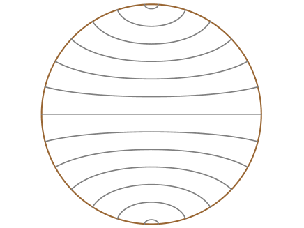
(a) AdS

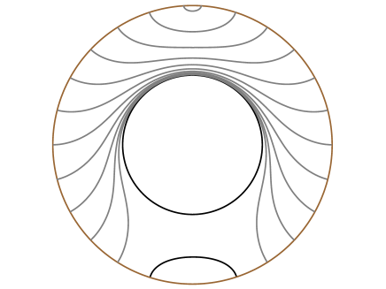
(b) AdS-Schwarzschild

Figure 1: Minimal-area surfaces.

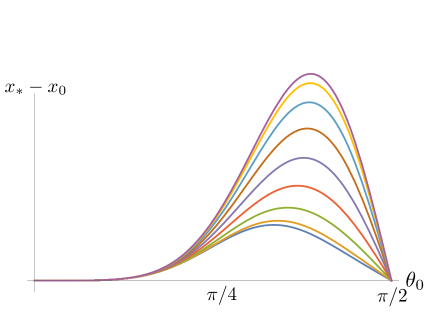
(a) $\Delta=4$

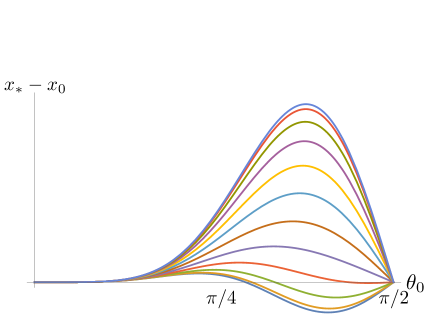
(b) $\Delta=3$

Figure 2: The change of the point at $\theta=0$ at different times.

To help understanding the change of the minimal-area surface in time, we plotted the change of the point at $\theta=0$ as a function of time in Fig.2. It is obvious from Fig.1(a) that for each curve, $\theta=0$ is the closest point to the center of AdS. Holographically speaking, $\theta=0$ points are thus the most IR point we can probe using HEE. Note that the perturbative computations are valid for small $\theta_{0}$ region, i.e. when the cap-like regions are small. The curves in Fig.2 represent how much the HEE curves are pushed away from the AdS origin, compared to the constant-latitude curve (3), due to the stress-energy tensor turned on by the nontrivial scalar field configuration. Another way of interpreting the time-dependence of our metric is that it should be at least qualitatively similar to the formation of black hole, due to a collapse of spherical shell. What we see in Fig.2 is the change of HEE in time, as a spherically symmetric shell starts from AdS infinity and shrinking to a point at the AdS center. We clearly see in Fig.2 that $x_{*}-x_{0}$ is smaller for $\Delta=3$, when compared to $\Delta=4$ case. It agrees with our intuition that when the scalar field is less massive (and more tachyonic), the effect on the gravitational system should be weaker and eventually the push-away effect should be also weaker.

IV Entanglement Temperature

One encounters a relation similar to the thermodynamical first law from the entanglement entropy in a small subsystem with excitations Bhattacharya:2012mi ; Allahbakhshi:2013rda ; Chakraborty:2014lfa ; Dey:2014voa ; Chakraborty:2014lfa ; Momeni:2015vka ; Ghoroku:2015apa ; Mishra:2015cpa ; Pal:2015mda ; Matsueda:2015bba ; Li:2015ola ; Mansoori:2015sit ; Park:2015hcz . Namely, the change of entanglement entropy and the energy are linearly related, and the entanglement temperature is defined as $T_{\text{ent}}\Delta S_{A}=\Delta E_{A}$. Since we consider small fluctuations and small entangling regions in this paper, let us also compute the entanglement temperature. We already computed $\Delta S_{A}$, so we only need to compute the change of energy $\Delta E_{A}$. It turns out that, for a small entangling region $A$, the entanglement temperature $T_{\text{ent}}$ is proportional to the inverse size of the subsystem, and the proportionality coefficient is determined by the shape of the entangling region and independent of the strength of the fluctuation. We take $AdS_{5}$ case for concreteness, but obviously the computation can be easily repeated in other dimensions.

IV.1 AdS-Schwarzschild black hole

In terms of Fefferman-Graham coordinates, asymptotically AdS metric is written as $ds^{2}=\frac{dz^{2}}{z^{2}}+\gamma_{ab}dx^{a}dx^{b}$. Then (15) is rewritten as follows Tetradis:2009bk ,

$$ds^{2}=\frac{1}{z^{2}}\biggl{[}dz^{2}-\frac{(1-\alpha_{1}z^{4})^{2}}{1+\alpha_{2}z^{2}+\alpha_{3}z^{4}}dt^{2}+(1+\alpha_{2}z^{2}+\alpha_{3}z^{4})(d\theta^{2}+\sin^{2}\theta\Omega_{2}^{2})\biggr{]},$$ (38)

where $\alpha_{1}=1,\alpha_{2}=-\frac{1}{2}$, and $\alpha_{3}=\frac{1+4M}{16}$. The new holographic coordinate and $z$ is defined by

$$\frac{dz}{z}=-\frac{dr}{\sqrt{f(r)}}\Longrightarrow z^{2}=\frac{4}{1+2r^{2}+2r\sqrt{f(r)}}.$$ (39)

Expanding the induced metric $\gamma_{ab}$ near the AdS boundary ($z=0$), one gets

$$\gamma_{ab}=\gamma_{(0)ab}+z^{2}\gamma_{(2)ab}+z^{4}\gamma_{(4)ab}+\cdots.$$ (40)

Then the stress tensor of the boundary theory is given by deHaro:2000xn ; Skenderis:2000in

$$T_{ab}^{\text{CFT}}=\frac{4}{16\pi G_{N}}\biggl{[}\gamma_{(4)ab}-\frac{1}{8}\gamma_{(0)ab}[(\text{Tr}\gamma_{(2)})^{2}-\text{Tr}\gamma_{(2)}^{2}]-\frac{1}{2}(\gamma_{(2)}^{2})_{ab}+\frac{1}{4}\gamma_{(2)ab}\text{Tr}\gamma_{(2)}\biggr{]},$$ (41)

which upon substitution of (38) becomes

$$T_{tt}=\frac{3\ell^{3}}{64\pi G_{N}}+M\frac{3\ell^{3}}{16\pi G_{N}}.$$ (42)

Here the first term on the right-hand side is the time-time component of the stress tensor of pure five-dimensional AdS spacetime (Casimir energy), and the second term is fluctuation energy for small black hole mass. At $r=\infty$ $(z=0)$ the metric (15) the boundary metric approaches $R\times S^{3}$. The energy is given by

$$\Delta E_{A} = \text{Vol}(S^{2})\int^{\theta_{0}}_{0}d\theta\sin^{2}\theta\times\Delta T_{tt}$$ (43)

$$= \frac{3(\cos^{-1}a-a\sqrt{1-a^{2}})}{8G_{5}}M,$$

where $a=\cos\theta_{0}$ and we have set $\ell=1$. Combining $\Delta E_{A}$ and $\Delta S_{A}$ and expand for small $\theta_{0}$ angle, we obtain

$$\frac{\Delta S_{A}}{\Delta E_{A}}=\frac{1}{T_{\text{ent}}}=\frac{4\pi}{5}\theta_{0}.$$ (44)

IV.2 AdS-Scalar systems

To compute the boundary stress tensor for AdS-scalar systems we employ the method used in Myers:1999psa . Let $\mathcal{M}$ be the spacetime manifold with time-like boundary $\partial\mathcal{M}$. The induced metric on the boundary is $\gamma_{\mu\nu}=g_{\mu\nu}-n_{\mu}n_{\nu}$, where $n^{\mu}$ is the outward-pointing normal vector normal to $\partial\mathcal{M}$. The extrinsic curvature on $\partial\mathcal{M}$ is then $\Theta_{\mu\nu}=-\gamma_{\mu}^{\;\;\rho}\nabla_{\rho}n_{\nu}$.

In five-dimensions, the Einstein action including the boundary term is given by

$$I=\frac{1}{16\pi G_{5}}\int_{\mathcal{M}}d^{5}x\sqrt{-g}(R-2\Lambda)-\frac{1}{8\pi G_{5}}\oint_{\partial\mathcal{M}}d^{4}x\sqrt{-\gamma}\Theta+I_{\text{matter}},$$ (45)

where $\Theta$ is the trace of the extrinsic curvature of the boundary. The boundary stress tensor is given by

$$\tau^{ab}\equiv\frac{2}{\sqrt{-\gamma}}\frac{\delta I}{\delta\gamma_{ab}}=\frac{1}{8\pi G_{N}}(\Theta^{ab}-\gamma^{ab}\Theta^{c}_{c}).$$ (46)

We need to regularize this action, and introduce a reference background metric $g^{0}_{\mu\nu}$ which asymptotically agrees with $g_{\mu\nu}$ on the boundary. The regularized action in this subtraction scheme is given by $\hat{I}=I(g)-I^{0}(g^{0})$ and a finite stress tensor is given by Hawking:1995fd

$$\hat{\tau}^{ab}\equiv\frac{2}{\sqrt{-\gamma}}\frac{\delta\hat{I}}{\delta\gamma_{ab}}=\tau^{ab}-(\tau^{0})^{ab}.$$ (47)

The stress tensor $\langle T\rangle_{ab}$ in the field theory is given, following the standard AdS/CFT dictionary, as

$$\sqrt{-h}h^{ab}\langle T\rangle_{bc}=\lim_{R\rightarrow\infty}\sqrt{-\gamma}\gamma^{ab}\hat{\tau}_{bc},$$ (48)

where $h_{ab}$ is the background metric for the field theory spacetime.

For our ansatz (7), the normal vector to the surface at $x=x_{0}$ is

$$n^{\mu}=\frac{\cos x_{0}}{\ell\sqrt{1+\lambda\Psi(t,x_{0})}}\delta^{\mu}_{x}.$$ (49)

In the standard ADM decomposion of the metric we read off

$$\gamma_{00}=-\frac{\ell^{2}(1+\lambda\Phi(t,x_{0}))}{\cos^{2}x_{0}},~{}~{}~{}~{}\gamma_{ij}=\ell^{2}\tan^{2}x_{0}\bar{\gamma}_{ij},$$ (50)

where $i,j=1,2,3$ and $\bar{\gamma}_{ij}$ is the metric on a unit 3-sphere. The computation is then straightforward, and we obtain

$$\hat{\tau}_{tt}=\frac{\ell\cos^{2}x_{0}\lambda}{8\pi G_{5}}+\cdots.$$ (51)

Finally using the relation (48) one arrives at

$$\langle T_{00}\rangle=\frac{\ell^{3}\lambda}{8\pi G_{5}},$$ (52)

which obviously gives the same entanglement temperature as (44). For the massive scalar fields $\Delta=3,2$ we have checked that the results are always the same as (44), verifying the statement in Bhattacharya:2012mi that the proportionality coefficient for entanglement entropy as a function of the subsystem size should be universal and does not depend on the details of the excitations.

V Discussions

In this paper, we have calculated the holographic entanglement entropy (HEE) perturbatively in the backgrounds which are small deformations of AdS vacuum. More concretely, we considered Schwarzschild black holes, and also harmonically driven time-dependent backgrounds. We chose the entanglement region to be cap-like ones around north pole of the boundary space. The motivation of this work was to see how small excitations in the gravity side manifest itself in HEE. Our observation is that the metric perturbation around the AdS vacuum does not affect the divergent terms and the change is in the finite part, as one expands with respect to the regularization parameter. We also considered the entanglement thermodynamics and computed the entanglement temperature for small sub-systems. This result is consistent with Ref.Bhattacharya:2012mi , where it was argued that the entanglement temperature should exhibit a universal feature which is proportional to the inverse size of the system. We have used the methods proposed in Myers:1999psa ; deHaro:2000xn to compute the boundary stress tensor and obtained the thermodynamic first-law like relation. We have checked that the proportional factor has always the same value for the system considered in this paper.

As a final comment, it would be also interesting to extend the study of time-dependent background and compute another thermodynamic quantity, the so-called entanglement pressure, which further generalizes the first law of thermodynamics for quantum entanglement Allahbakhshi:2013rda .

- (1) G. ’t Hooft, Dimensional reduction in quantum gravity, in Salamfest 1993:0284-296, pp. 0284–296, 1993. gr-qc/9310026.
- (2) L. Susskind, The World as a hologram, J. Math. Phys. 36 (1995) 6377–6396, [hep-th/9409089].
- (3) J. M. Maldacena, The Large N limit of superconformal field theories and supergravity, Adv.Theor.Math.Phys. 2 (1998) 231–252, [hep-th/9711200].
- (4) S. Ryu and T. Takayanagi, Holographic derivation of entanglement entropy from AdS/CFT, Phys. Rev. Lett. 96 (2006) 181602, [hep-th/0603001].
- (5) B. Swingle, Entanglement Renormalization and Holography, Phys. Rev. D86 (2012) 065007, [arXiv:0905.1317].
- (6) G. Vidal, Entanglement Renormalization, Phys. Rev. Lett. 99 (2007), no. 22 220405, [cond-mat/0512165].
- (7) V. E. Hubeny, M. Rangamani, and T. Takayanagi, A Covariant holographic entanglement entropy proposal, JHEP 0707 (2007) 062, [arXiv:0705.0016].
- (8) V. Balasubramanian, A. Bernamonti, J. de Boer, N. Copland, B. Craps, E. Keski-Vakkuri, B. Muller, A. Schafer, M. Shigemori, and W. Staessens, Thermalization of Strongly Coupled Field Theories, Phys. Rev. Lett. 106 (2011) 191601, [arXiv:1012.4753].
- (9) V. Balasubramanian, A. Bernamonti, J. de Boer, N. Copland, B. Craps, E. Keski-Vakkuri, B. Muller, A. Schafer, M. Shigemori, and W. Staessens, Holographic Thermalization, Phys. Rev. D84 (2011) 026010, [arXiv:1103.2683].
- (10) V. Balasubramanian, A. Bernamonti, N. Copland, B. Craps, and F. Galli, Thermalization of mutual and tripartite information in strongly coupled two dimensional conformal field theories, Phys. Rev. D84 (2011) 105017, [arXiv:1110.0488].
- (11) A. Allais and E. Tonni, Holographic evolution of the mutual information, JHEP 01 (2012) 102, [arXiv:1110.1607].
- (12) V. Keranen, E. Keski-Vakkuri, and L. Thorlacius, Thermalization and entanglement following a non-relativistic holographic quench, Phys. Rev. D85 (2012) 026005, [arXiv:1110.5035].
- (13) E. Caceres and A. Kundu, Holographic Thermalization with Chemical Potential, JHEP 09 (2012) 055, [arXiv:1205.2354].
- (14) W. Baron, D. Galante, and M. Schvellinger, Dynamics of holographic thermalization, JHEP 1303 (2013) 070, [arXiv:1212.5234].
- (15) V. E. Hubeny, M. Rangamani, and E. Tonni, Thermalization of Causal Holographic Information, JHEP 05 (2013) 136, [arXiv:1302.0853].
- (16) H. Liu and S. J. Suh, Entanglement Tsunami: Universal Scaling in Holographic Thermalization, Phys. Rev. Lett. 112 (2014) 011601, [arXiv:1305.7244].
- (17) H. Liu and S. J. Suh, Entanglement growth during thermalization in holographic systems, Phys. Rev. D89 (2014), no. 6 066012, [arXiv:1311.1200].
- (18) V. E. Hubeny and H. Maxfield, Holographic probes of collapsing black holes, JHEP 03 (2014) 097, [arXiv:1312.6887].
- (19) M. Alishahiha, M. R. M. Mozaffar, and M. R. Tanhayi, On the Time Evolution of Holographic n-partite Information, JHEP 09 (2015) 165, [arXiv:1406.7677].
- (20) X. Bai, B.-H. Lee, L. Li, J.-R. Sun, and H.-Q. Zhang, Time Evolution of Entanglement Entropy in Quenched Holographic Superconductors, arXiv:1412.5500.
- (21) E. da Silva, E. Lopez, J. Mas, and A. Serantes, Collapse and Revival in Holographic Quenches, JHEP 04 (2015) 038, [arXiv:1412.6002].
- (22) Y. Nakaguchi, N. Ogawa, and T. Ugajin, Holographic Entanglement and Causal Shadow in Time-Dependent Janus Black Hole, arXiv:1412.8600.
- (23) V. Keranen, H. Nishimura, S. Stricker, O. Taanila, and A. Vuorinen, Gravitational collapse of thin shells: Time evolution of the holographic entanglement entropy, JHEP 06 (2015) 126, [arXiv:1502.01277].
- (24) V. Ziogas, Holographic mutual information in global Vaidya-BTZ spacetime, JHEP 09 (2015) 114, [arXiv:1507.00306].
- (25) S. Leichenauer, Thermal Corrections to Entanglement Entropy from Holography, arXiv:1502.07348.
- (26) R. Mishra and H. Singh, Perturbative entanglement thermodynamics for AdS spacetime: Renormalization, arXiv:1507.03836.
- (27) M. Maliborski and A. Rostworowski, Time-Periodic Solutions in an Einstein AdS–Massless-Scalar-Field System, Phys. Rev. Lett. 111 (2013) 051102, [arXiv:1303.3186].
- (28) N. Kim, Time-periodic solutions of massive scalar fields in dynamical AdS background: Perturbative constructions, Phys.Lett. B742 (2015) 274–278, [arXiv:1411.1633].
- (29) I. Bakas and G. Pastras, Entanglement Entropy and Duality in AdS(4), arXiv:1503.00627.
- (30) T. Takayanagi, Entanglement Entropy from a Holographic Viewpoint, Class. Quant. Grav. 29 (2012) 153001, [arXiv:1204.2450].
- (31) T. Nishioka, S. Ryu, and T. Takayanagi, Holographic Entanglement Entropy: An Overview, J. Phys. A42 (2009) 504008, [arXiv:0905.0932].
- (32) P. Bizon and A. Rostworowski, On weakly turbulent instability of anti-de Sitter space, Phys.Rev.Lett. 107 (2011) 031102, [arXiv:1104.3702].
- (33) G. Fodor, P. Forgács, and P. Grandclément, Self-gravitating scalar breathers with negative cosmological constant, arXiv:1503.07746.
- (34) V. E. Hubeny, H. Maxfield, M. Rangamani, and E. Tonni, Holographic entanglement plateaux, JHEP 1308 (2013) 092, [arXiv:1306.4004].
- (35) B. Craps, O. Evnin, and J. Vanhoof, Renormalization group, secular term resummation and AdS (in)stability, JHEP 1410 (2014) 48, [arXiv:1407.6273].
- (36) B. Craps, O. Evnin, and J. Vanhoof, Renormalization, averaging, conservation laws and AdS (in)stability, JHEP 1501 (2015) 108, [arXiv:1412.3249].
- (37) J. Bhattacharya, M. Nozaki, T. Takayanagi, and T. Ugajin, Thermodynamical Property of Entanglement Entropy for Excited States, Phys. Rev. Lett. 110 (2013), no. 9 091602, [arXiv:1212.1164].
- (38) D. Allahbakhshi, M. Alishahiha, and A. Naseh, Entanglement Thermodynamics, JHEP 1308 (2013) 102, [arXiv:1305.2728].
- (39) S. Chakraborty, P. Dey, S. Karar, and S. Roy, Entanglement thermodynamics for an excited state of Lifshitz system, JHEP 04 (2015) 133, [arXiv:1412.1276].
- (40) A. Dey, S. Mahapatra, and T. Sarkar, Very General Holographic Superconductors and Entanglement Thermodynamics, JHEP 12 (2014) 135, [arXiv:1409.5309].
- (41) D. Momeni, M. Raza, H. Gholizade, and R. Myrzakulov, Realization of Holographic Entaglement Temperature for a Nearly-AdS Boundary, arXiv:1505.00215.
- (42) K. Ghoroku and M. Ishihara, Entanglement temperature for the excitation of SYM theory in the (de)confinement phase, Phys. Rev. D92 (2015), no. 8 085017, [arXiv:1506.06474].
- (43) S. S. Pal and S. Panda, Entanglement temperature with Gauss–Bonnet term, Nucl. Phys. B898 (2015) 401–414, [arXiv:1507.06488].
- (44) H. Matsueda, Hessian potential for Fefferman-Graham metric, arXiv:1508.06515.
- (45) G.-Q. Li, J.-X. Mo, and X.-B. Xu, Entanglement temperature for black branes with hyperscaling violation, arXiv:1509.05985.
- (46) S. A. H. Mansoori, B. Mirza, M. D. Darareh, and S. Janbaz, Entanglement Thermodynamics of the Generalized Charged BTZ Black Hole, arXiv:1512.00096.
- (47) C. Park, Thermodynamic law from the entanglement entropy bound, arXiv:1511.02288.
- (48) N. Tetradis, The Temperature and entropy of CFT on time-dependent backgrounds, JHEP 03 (2010) 040, [arXiv:0905.2763].
- (49) S. de Haro, S. N. Solodukhin, and K. Skenderis, Holographic reconstruction of space-time and renormalization in the AdS / CFT correspondence, Commun. Math. Phys. 217 (2001) 595–622, [hep-th/0002230].
- (50) K. Skenderis, Asymptotically Anti-de Sitter space-times and their stress energy tensor, Int. J. Mod. Phys. A16 (2001) 740–749, [hep-th/0010138].
- (51) R. C. Myers, Stress tensors and Casimir energies in the AdS / CFT correspondence, Phys. Rev. D60 (1999) 046002, [hep-th/9903203].
- (52) S. W. Hawking and G. T. Horowitz, The Gravitational Hamiltonian, action, entropy and surface terms, Class. Quant. Grav. 13 (1996) 1487–1498, [gr-qc/9501014].