Lively quantum walks on cycles

Abstract

We introduce a family of quantum walks on cycles parametrized by their liveliness, defined by the ability to execute a long-range move. We investigate the behaviour of the probability distribution and time-averaged probability distribution. We show that the liveliness parameter, controlling the magnitude of the additional long-range move, has a direct impact on the periodicity of the limiting distribution. We also show that the introduced model provides a method for network exploration which is robust against trapping.

Keywords: quantum walks, Markov processes, limiting distribution

PACS: 03.67.-a, 05.40.Fb, 02.50.Ga

1 Introduction

Quantum walks [1, 2, 3], quantum counterparts of classical Markov processes, provide a powerful method for developing new quantum algorithms [4] and protocols [5, 6, 7, 8, 9]. As quantum protocols have to be executed on pair with classical protocols controlling distant parts of a quantum network, quantum walks have to include elements enabling them to adapt to the current structure of the network. The methods of adapting classical algorithms for the purpose of quantum networks are currently under an active investigation [10] and include the application of game theory in a complex quantum network with interacting parties [11].

Quantum walks on cycles can be used as a simple and very powerful model for the purpose of modeling quantum and hybrid classical-quantum networks. In particular, in [7], the authors have developed a model that can be used to analyze the scenario of exploring quantum networks with a distracted sense of direction. By using this model, it is possible to study the behavior of quantum mobile agents operating with non-adaptive and adaptive strategies that can be employed in this scenario.

The presented work introduces a family of quantum walks on cycles with liveliness, corresponding to the ability to execute a long-range move. The introduced family is parametrized by the liveliness parameter, which is used to control the magnitude of the additional long-range move. In particular, the proposed family contains lazy quantum walks, which can be introduced as quantum walks with liveliness equal to 0. We investigate the behavior of the probability distribution and time-averaged probability distribution [12] for the introduced family and generalize the results obtained by Bednarska et al. [13]. We show that the liveliness parameter has a direct impact on the periodicity of the limiting distribution. We also show that the introduced model provides a method for network exploration which is robust against trapping.

This paper is organized as follows. In Section 2 we introduce the model of lively quantum walks on cycles. In Section 3 we study the behavior of the time-averaged limiting distribution of the introduced model and discuss its periodicity. In Section 4 we prove that the introduced model allows the improvement of the quantum network exploration. This is achieved by demonstrating that our model can be used to avoid trapping and to counteract malfunctions in the network. Finally, in Section 5, we discuss the possible applications and extensions of the introduced model.

2 Lively quantum walks

Let us first consider a cycle with $n$ nodes and define a standard model of quantum walk. The position of a walker during a quantum walk executed on such cycle is described by a vector in $n$-dimensional complex space $\mathds{C}^{n}$. The state space is of the form $\mathds{C}^{2}\otimes\mathds{C}^{n}$. Quantum walk process is defined in the situation by the shift operator

$$\begin{split}S(|0\rangle\otimes|i\rangle)&=|0\rangle\otimes|i+1\pmod{n}\rangle,\\ S(|1\rangle\otimes|i\rangle)&=|1\rangle\otimes|i-1\pmod{n}\rangle,\end{split}$$ (1)

or equivalently

$$S=|0\rangle\langle 0|\otimes\sum\limits_{i=0}^{n-1}|i+1\rangle\langle i|+|1\rangle\langle 1|\otimes\sum\limits_{i=0}^{n-1}|i-1\rangle\langle i|,$$ (2)

where addition is modulo $n$. In this case the walker has for her disposal two directions – $|0\rangle$ (right) and $|1\rangle$ (left) – represented in the two dimensional Hilbert space $\mathds{C}^{2}$, corresponding to the coin used in the classical random walk. The evolution operator is defined as

$$U=S(C\otimes{\rm 1l}_{n}),$$ (3)

where $C$ is the coin operator which acts on coin space $\mathds{C}^{2}$.

Let us now assume that the coin register used to control a quantum walker is represented by a vector in $\mathds{C}^{3}$ (i.e. by a qutrit) and thus, during each step, the walker can change its position according to one of three possible states of the coin register. Using this setup we define lively quantum walk on cycles as follows.

Definition 1 (Lively quantum walk on a cycle)

Lively quantum walk on a $n$-dimensional cycle with liveliness $0\leq a\leq n-1$, is defined by the shift operator $S^{(n,a)}\in L(\mathds{C}^{3}\otimes\mathds{C}^{n})$ of the form

$$S^{(n,a)}=\sum_{x=0}^{n-1}S_{x}^{(n,a)},$$ (4)

where

$$\begin{split}S_{x}^{(n,a)}&=|0\rangle\langle 0|\otimes|x-1\pmod{n}\rangle\langle x|\\ &+|1\rangle\langle 1|\otimes|x+1\pmod{n}\rangle\langle x|\\ &+|2\rangle\langle 2|\otimes|x+a\pmod{n}\rangle\langle x|.\end{split}$$ (5)

For the case $a=0$ the above definition reduces to lazy quantum walk (i.e. a quantum walk with no liveliness). One should also note that if the introduced model would included jumps with $-a$ parameter we could restrict our considerations to the case where $a\leq\lfloor\frac{n}{2}\rfloor$.

For the small number of nodes, the existence of the additional connections can be used to model the transition from a cycle to the full network. For example, for $n=6$, the lively quantum walk with $a=2$ is equivalent to the quantum walk on the total network. However, in order to study the parametrized family of processes on graphs with different degree of connectivity, additional connections, and thus larger coins, are needed.

Operator $S_{x}^{(n,a)}$ acts on position $x$ by shifting it by $+1$, $-1$ or by the value specified by the liveliness parameter $a\in\{0,1,\dots,n-1\}$. The case $a=0$ is identical to the case $a=n$.

The coin operator used in the further considerations is defined by the Grover operator

$$G=2|c_{1}\rangle\langle c_{1}|-{\rm 1l}_{3}=\left(\begin{smallmatrix}-\frac{1}{3}&\frac{2}{3}&\frac{2}{3}\\ \frac{2}{3}&-\frac{1}{3}&\frac{2}{3}\\ \frac{2}{3}&\frac{2}{3}&-\frac{1}{3}\\ \end{smallmatrix}\right),$$ (6)

where

$$|c_{1}\rangle=\frac{1}{\sqrt{3}}\left(|0\rangle+|1\rangle+|2\rangle\right).$$ (7)

Using the above we define the walk operator for the lively walk on cycle as

$$U=\left(\sum_{x=0}^{n-1}S_{x}^{(n,a)}\right)(G\otimes{\rm 1l}_{n}).$$ (8)

3 Limiting distribution periodicity

We start with the proof of the periodicity of the limiting distribution for the introduced model. Let us introduce the time-averaged probability distribution for the quantum walk as follows.

Definition 2

We define the time-averaged probability distribution at position $x$ for a unitary process $U$ as

$$\Pi(x)=\lim_{N\rightarrow\infty}\frac{1}{N}\sum_{t=0}^{N}P(x,t),$$ (9)

where $P(x,t)$ denotes the probability of measuring position $x$ after $t$ steps

$$P(x,t)=\sum_{c=0}^{2}|\langle c,x|U^{t}|\psi_{0}\rangle|^{2}$$ (10)

and $|\psi_{0}\rangle$ is arbitrary initial state.

Let us now consider a lively quantum walk with $n$ nodes and the step size $a$ chosen in such a way that there is a common divisor of both numbers.

Theorem 1

If $\mathrm{GCD}(a,n)>1$ then the limiting time-averaged probability distribution is periodic with period equal to $\mathrm{GCD}(a,n)$.

First, let us note that the spectrum of the walk operator is conveniently expressed using Fourier basis at the position register.

Lemma 1

The walk operator $U=S^{(n,a)}(G\otimes{\rm 1l}_{n})\in L(\mathds{C}^{3}\otimes\mathds{C}^{n})$ has eigenvalues $\lambda_{k,j}$ with corresponding eigenvectors $|\psi_{k,j}\rangle=|v_{k,j}\rangle\otimes|\phi_{k}\rangle\in\mathds{C}^{3}\otimes\mathds{C}^{n}$ satisfying the equation

$$\operatorname{diag}(e^{-\mathrm{i}k},e^{\mathrm{i}k},e^{-\mathrm{i}ka})G|v_{k,j}\rangle=\lambda_{k,j}|v_{k,j}\rangle,$$ (11)

where $|\phi_{k}\rangle=\sum e^{-\mathrm{i}kx}|x\rangle$ for $k=\frac{2\pi l}{n},l=0,\ldots,n-1$, $j\in\{0,1,2\}$.

Proof. We analyse the action of the step on $|d\rangle\otimes|\phi_{k}\rangle$ for basis state $d\in\{0,1,2\}$ and note that the step operator acting on states with Fourier states on position register results in a relative phase $S^{(n,a)}|0\rangle\otimes|\phi_{k}\rangle=e^{\mathrm{i}k}|0\rangle\otimes|\phi_{k}\rangle$, $S^{(n,a)}|1\rangle\otimes|\phi_{k}\rangle=e^{-\mathrm{i}k}|1\rangle\otimes|\phi_{k}\rangle$ and $S^{(n,a)}|2\rangle\otimes|\phi_{k}\rangle=e^{-\mathrm{i}ka}|2\rangle\otimes|\phi_{k}\rangle$. Thus we can reduce the dynamics of the states of the form $|v\rangle\otimes|\phi_{k}\rangle$ so that we consider the $|v\rangle$ subsystem only and we substitute the step operator with $\operatorname{diag}(e^{-\mathrm{i}k},e^{\mathrm{i}k},e^{-\mathrm{i}ka})$. Therefore any eigenvector $|v_{k,j}\rangle$ of the form given in Eq. (11) corresponds to an eigenvector of the form $|v_{k,j}\rangle\otimes|\phi_{k}\rangle$ of the walk operator $U$.  

In the context of the limiting distribution we emphasise the fact that for any eigenvector of the form $|\psi_{k,j}\rangle=|v_{k,j}\rangle\otimes|\phi_{k}\rangle$ the probability distribution at the coin register

$$|(\langle d|\otimes\langle x|)|\psi_{k,j}\rangle|^{2}=|\langle{d}|{v_{k,j}}\rangle|^{2}$$ (12)

is position independent. This property can be applied into limiting distribution formula

$$\Pi(x)=\sum_{\lambda}\sum_{d}\sum_{(k,j),(k^{\prime},j^{\prime})\in V_{\lambda}}a_{k,j}^{\phantom{*}}a_{k^{\prime},j^{\prime}}^{*}\langle{d,x}|{\psi_{k,j}}\rangle\langle{\psi_{k^{\prime},j^{\prime}}}|{d,x}\rangle,$$ (13)

where $x$ is the position, $|\psi_{0}\rangle=\sum a_{k,l}|\psi_{k,l}\rangle$, $V_{\lambda}$ are indices of $\lambda$-eigenvectors such that $V_{\lambda}=\{(k,j):\lambda_{k,j}=\lambda\}$. It is straightforward from Eq. (12) that for 1-dimensional eigenspaces the probability is transition invariant

$$a_{k,j}^{\phantom{\dagger}}a_{k,j}^{*}\langle{d,x}|{\psi_{k,j}}\rangle\langle{\psi_{k,j}}|{d,x}\rangle=a_{k,j}^{\phantom{\dagger}}a_{k,j}^{*}|\langle{d}|{v_{k,j}}\rangle|^{2}=a_{k,j}^{\phantom{\dagger}}a_{k,j}^{*}\langle{d,x^{\prime}}|{\psi_{k,j}}\rangle\langle{\psi_{k,j}}|{d,x^{\prime}}\rangle,$$ (14)

for $x,x^{\prime}=1,\dots,n$. For higher-dimensional eigenspaces we are concerned with relative phase during transition. In other words, one is assured that for two positions $x,x^{\prime}$ the modules of the terms $\langle{d,x}|{\psi_{i}}\rangle\langle{\psi_{j}}|{d,x}\rangle$ and $\langle{d,x^{\prime}}|{\psi_{i}}\rangle\langle{\psi_{j}}|{d,x^{\prime}}\rangle$ are equal, however they may differ in phase. Here we prove that the dimensionality of eigenspaces of eigenvalues $\lambda_{k,j}$ is higher than one if the relation $k=\frac{2\pi}{n}l$ is satisfied for $l$ being the multiplication of $\frac{n}{\mathrm{GCD}(n,a)}$. We do not prove that for $k\neq\frac{2\pi l}{\mathrm{GCD}(n,a)}$ the $\lambda_{k,j}$-eigenspace is one-dimensional, but the influence of the cases when it is not true is negligible.

Lemma 2

For $k=\frac{2\pi l}{n}$ and $\frac{n}{\mathrm{GCD}(n,a)}|l$ we have that $\lambda_{k,0}=1$ is an eigenvalue of $U$ and the other eigenvalues $\lambda_{k,1}$, $\lambda_{k,2}$ are mutually conjugated i.e. $\lambda_{k,1}\lambda_{k,2}=1$. Moreover, eigenvalues for $k^{\prime}=2\pi-k$ are the same.

Proof. Let us derive the characteristic polynomial for eigenvalues of the step operator on the subspace corresponding to the $|\phi_{k}\rangle$ on the position space

$$\overline{U_{k}}=\operatorname{diag}(e^{-\mathrm{i}k},e^{\mathrm{i}k},e^{-\mathrm{i}ka})G.$$ (15)

From assumptions we obtain that $n|la$ and thus $e^{\mathrm{i}ka}=1$. Thus the characteristic polynomial simplifies to

$$(1-\lambda)\left(\frac{\lambda}{3}(1-2\cos k)+1+\lambda+\lambda^{2}\right),$$ (16)

with real coefficients and the same solution for $-k$ thus $\lambda_{0}=1$ and lemma holds. The explicit formulas for the eigenvalues with substitution for $e^{\mathrm{i}k}=\omega$ are

$$\left\{1,-\frac{\omega^{2}+4\omega+(\omega-1)\sqrt{\omega(\omega+10)+1}+1}{6\omega},-\frac{\omega^{2}+4\omega-(\omega-1)\sqrt{\omega(\omega+10)+1}+1}{6\omega}\right\}$$

and eigenvectors without normalization factors read

$$\left(\begin{array}[]{ccc}\frac{2}{\omega+1}&\frac{2\omega}{\omega+1}&1\\ \frac{-\omega+\sqrt{\omega(\omega+10)+1}-1}{4\omega}&\frac{1}{4}\left(-\omega-\sqrt{\omega(\omega+10)+1}-1\right)&1\\ -\frac{\omega+\sqrt{\omega(\omega+10)+1}+1}{4\omega}&\frac{1}{4}\left(-\omega+\sqrt{\omega(\omega+10)+1}-1\right)&1\\ \end{array}\right)$$ (17)

 

Proof of Theorem 1. In order to prove the cyclic property of the walk we consider the limiting distribution from Def, 2 in the alternative form

$$\Pi(x)=\sum_{\lambda}\sum_{(k,j),(k^{\prime},j^{\prime})\in V_{\lambda},d}a_{k,j}^{\phantom{*}}a_{k^{\prime},j^{\prime}}^{*}\langle{d,x}|{\psi_{k,j}}\rangle\langle{\psi_{k^{\prime},j^{\prime}}}|{d,x}\rangle.$$ (18)

We aim at proving that $\Pi(x)=\Pi(x+a)$. We note that for each eigenvalue $\lambda$ such that $|V_{\lambda}|=1$ its unique eigenvector $|\psi_{k,j}\rangle$ satisfies $|\langle{d,x}|{\psi_{k,j}}\rangle|^{2}=|\langle{d,x+a}|{\psi_{k,j}}\rangle|^{2}$ as a result of Lemma 1. We assume that multiple eigenvalues $\lambda_{k,j}=\lambda_{k^{\prime},j^{\prime}}$ follow the case $k=\frac{2\pi l}{\mathrm{GCD}(a,n)},k^{\prime}=\frac{2\pi(n-l)}{\mathrm{GCD}(a,n)}$ resulting from construction in Lemma 2 and give the $e^{\mathrm{i}ka}=e^{\mathrm{i}k^{\prime}a}=1$ and $e^{\mathrm{i}k}e^{\mathrm{i}k^{\prime}}=1$. In particular, we show that the relative phases that occur in the terms of the sum Eq. (18) vanish every $a$ steps. Thus the equality

$$\langle{d,x+a}|{\psi_{k,j}}\rangle\langle{\psi_{k^{\prime},j^{\prime}}}|{d,x+a}\rangle=\langle{d,x}|{\psi_{k,j}}\rangle\langle{\psi_{k^{\prime},j^{\prime}}}|{d,x}\rangle$$ (19)

holds for $(k,j),(k^{\prime},j^{\prime})\in V_{\lambda}$ and overall limiting probability is periodic with the period equal to $\mathrm{GCD}(a,n)$.  

Thus, we observe interesting phenomena that if the paths generated by the lively steps do not interact i.e. create separate classes of nodes, then the asymptotic probabilities become equal within these classes. This behavior is illustrated in Fig. 1. One should note that the values of the limiting distribution depends on the initial state. However, the periodicity is not affected by the initial state.

(a) Aperiodic case

(b) Periodic case

Figure 1: Illustration of the simple networks for the lively walk with $n=6$ and $n=7$ nodes and the liveliness $a=2$. In the case 1(a) all nodes belong to the same class. In the case 1(b) red (dotted) and blue (dot-dashed) links connect the nodes corresponding to different classes exhibiting different asymptotic behavior.

4 Additional properties of lively walks

In this section we focus on some additional properties of the introduced model. We start by demonstrating that the model enables us to avoid the trapping of the particle for any coin. Next we study how the periodicity of the lively walks is disturbed if one of the links in the network is missing.

4.1 Mean difference of position

Let us consider the situation when we have two parties (or players) using the introduced model to execute a quantum walk on a network. The first player aims at exploring the network, whilst the other one aims at stopping the exploration by trapping the quantum walk. The second party can choose the coin used during the walk. Below we demonstrate that in such situation the introduced model is not vulnerable for the actions of the second party and the trapping can be avoided for any coin.

To be more precise we introduce a random variable $(X^{\rho},D^{\rho})$ that models the measurement in canonical basis of the joint position and coin register. Using this concept trapping of a quantum walk would mean that the probability distribution of the variable $X^{\rho_{t}}$, for $\rho_{t}$ being the state of the system in time $t$, does not change in time. In particular the expectation value $\mathbb{E}(X^{\rho_{t}})$ would be time-independent. Thus, in order to avoid trapping we will ensure that the expectation value of the position changes in time.

Theorem 2

Let $\mathcal{H}_{C}=\mathbb{C}^{3}$, $\mathcal{H}_{P}=\mathbb{C}^{n}$ be Hilbert spaces and $\mathcal{D}(\mathcal{H}_{C})$ and $\mathcal{D}(\mathcal{H}_{P})$ spaces of density operators corresponding to them. Let us suppose that we have a lively walk with an initial state $\rho_{0}\in\mathcal{D}(\mathcal{H}_{C}\otimes\mathcal{H}_{P})$ in the form $\rho_{0}=\frac{1}{3}(|0\rangle\langle 0|+|1\rangle\langle 1|+|2\rangle\langle 2|)\otimes{|x_{0}\rangle\langle x_{0}|}$. Then for arbitrary (time-dependent) three-dimensional coin operator $C_{t}$ the lively walk with liveliness $a\neq 0$, can not be trapped i.e. the difference of the expectation value of the position $\mathbb{E}(X^{\rho_{t+1}})-\mathbb{E}(X^{\rho_{t}})$ in time $t$ is non-zero.

One should note that in principle $C_{t}$ can change at each step of the evolution. For this reason this theorem can be applied for the model with the time-dependent coin operator.

Proof. First, we note that the shift operator from Eq. (4) may be represented in a different form

$$S^{(n,a)}=\sum\limits_{c=0}^{2}|c\rangle\langle c|\otimes U_{c}^{(n,a)},$$ (20)

where $U_{c}^{(n,a)}=\sum_{x}|x+\Delta_{c}^{(a)}\rangle\langle x|$, $\Delta_{c}^{(a)}=-\delta_{c,0}+\delta_{c,1}+a\delta_{c,2}$ and we perform addition modulo $n$. We also note that each pair of matrices $U_{c}^{(n,a)}$ commute. Let $\{|e_{m}\rangle\}_{m=1}^{n}$ be eigenvectors of matrices $U_{c}^{(n,a)}$. By mathematical induction we will show that state after arbitrary number of evolutions is of the form

$$\rho=\sum\limits_{ij}\sum\limits_{ml}\rho_{ij,ml}|i\rangle\langle j|\otimes|e_{m}\rangle\langle e_{l}|,$$ (21)

where

$$\rho_{ij,mm}=\frac{1}{3}\delta_{ij}a_{m}\textrm{ with }\ a_{m}=\langle{e_{m}}|{x_{0}}\rangle\langle{x_{0}}|{e_{m}}\rangle\textrm{ and }\ \sum\limits_{m}a_{m}=1.$$ (22)

Let us show that the relation in Eq. (22) are valid for the initial state. Matrix elements of $\rho_{0}$ are of the form

$$\begin{split}\langle i,e_{m}|\rho_{0}|j,e_{m}\rangle&=\langle i,e_{m}|\left(\frac{{\rm 1l}_{3}}{3}\otimes|x_{0}\rangle\langle x_{0}|\right)|j,e_{m}\rangle\\ &=\frac{1}{3}\langle{i}|{j}\rangle\otimes\langle{e_{m}}|{x_{0}}\rangle\langle{x_{0}}|{e_{m}}\rangle=\frac{1}{3}a_{m}\delta_{ij},\end{split}$$ (23)

where $|i\rangle,|j\rangle$, $i,j=0,1,2$, are the states of the canonical coin basis.

Next we will demonstrate inductive step.

$$\begin{split}\langle i,e_{m}|U\rho U^{\dagger}|j,e_{m}\rangle&=\langle i,e_{m}|S^{(n,a)}(C_{t}\otimes{\rm 1l}_{n})\rho(C_{t}^{\dagger}\otimes{\rm 1l}_{n})S^{(n,a)\dagger}|j,e_{m}\rangle\\ &=e^{\mathrm{i}\alpha_{i,m}}\langle i,e_{m}|(C_{t}\otimes{\rm 1l}_{n})\rho(C_{t}^{\dagger}\otimes{\rm 1l}_{n})|j,e_{m}\rangle e^{-\mathrm{i}\alpha_{j,m}}\\ &=e^{\mathrm{i}(\alpha_{i,m}-\alpha_{j,m})}\sum\limits_{c,c^{\prime}}(\langle i|C_{t}|c\rangle\langle c,e_{m}|)\rho(\langle c^{\prime}|C_{t}^{\dagger}|j\rangle|c^{\prime},e_{m}\rangle)\\ &=e^{\mathrm{i}(\alpha_{i,m}-\alpha_{j,m})}\sum\limits_{c,c^{\prime}}\langle i|C_{t}|c\rangle\langle c^{\prime}|C_{t}^{\dagger}|j\rangle\langle c,e_{m}|\rho|c^{\prime},e_{m}\rangle\\ &=e^{\mathrm{i}(\alpha_{i,m}-\alpha_{j,m})}\frac{1}{3}a_{m}\sum\limits_{c}\langle i|C_{t}|c\rangle\langle c|C_{t}^{\dagger}|j\rangle\\ &=e^{\mathrm{i}(\alpha_{i,m}-\alpha_{j,m})}\frac{1}{3}a_{m}\delta_{ij}=\frac{1}{3}a_{m}\delta_{ij},\end{split}$$ (24)

where $e^{\mathrm{i}\alpha_{i,m}}$ is eigenvalue of $S$ which is corresponding to eigenvector $|i,e_{m}\rangle$.

Now we can show that the state from Eq. (21) after partial trace on position register is of the form $\frac{{\rm 1l}_{3}}{3}$.

$$\begin{split}\operatorname{tr}_{P}(\rho)&=\sum\limits_{k}{\rm 1l}_{3}\otimes\langle e_{k}|\Big{(}\sum\limits_{ij}\sum\limits_{ml}\rho_{ij,ml}|i\rangle\langle j|\otimes|e_{m}\rangle\langle e_{l}|\Big{)}{\rm 1l}_{3}\otimes|e_{k}\rangle\\ &=\sum\limits_{k}\sum\limits_{ij}\sum\limits_{ml}\rho_{ij,ml}|i\rangle\langle j|\langle{e_{k}}|{e_{m}}\rangle\langle{e_{l}}|{e_{k}}\rangle\\ &=\sum\limits_{ij}\sum\limits_{m}\frac{1}{3}a_{m}\delta_{ij}|i\rangle\langle j|=\frac{{\rm 1l}_{3}}{3}.\end{split}$$ (25)

The above result implies that after an arbitrary number of steps, a quantum walker moves right, left or jumps with equal probabilities.

Let $X^{\rho_{t}},D^{\rho_{t}}$ be random variables corresponding to the measurement on the position and coin register after $t$ steps, respectively. Furthermore let $\rho_{t}^{C}=(C\otimes{\rm 1l}_{n})\rho_{t}(C\otimes{\rm 1l}_{n})^{\dagger}.$ We have

$$\begin{split}\mathbb{E}(X^{\rho_{t+1}})&=\frac{1}{3}\mathbb{E}(X^{\rho_{t+1}}|D^{\rho_{t+1}}=0)+\frac{1}{3}\mathbb{E}(X^{\rho_{t+1}}|D^{\rho_{t+1}}=1)+\frac{1}{3}\mathbb{E}(X^{\rho_{t+1}}|D^{\rho_{t+1}}=2)\\ &=\frac{1}{3}\Big{(}\mathbb{E}(X^{\rho_{t}^{C}}|D^{\rho_{t}^{C}}=0)-1\Big{)}+\frac{1}{3}\Big{(}\mathbb{E}(X^{\rho_{t}^{C}}|D^{\rho_{t}^{C}}=1)+1\Big{)}+\frac{1}{3}\Big{(}\mathbb{E}(X^{\rho_{t}^{C}}|D^{\rho_{t}^{C}}=2)+a\Big{)}\\ &=\frac{1}{3}\Big{(}\mathbb{E}(X^{\rho_{t}^{C}}|D^{\rho_{t}}=0)+\mathbb{E}(X^{\rho_{t}^{C}}|D^{\rho_{t}}=1)+\mathbb{E}(X^{\rho_{t}^{C}}|D^{\rho_{t}}=2)\Big{)}+\frac{1}{3}\Big{(}-1+1+a\Big{)}\\ &=\mathbb{E}(X^{\rho_{t}^{C}})+\frac{1}{3}(-1+1+a)\\ &=\mathbb{E}(X^{\rho_{t}})+\frac{a}{3},\end{split}$$ (26)

where $P(D^{\rho_{t+1}}=i)=\frac{1}{3}$ for all $i\in\{0,1,2\}$. This proves the claim.  

One should note that this enables the user to obtain an arbitrary change of position. This does not depend on whether the $\mathrm{GCD}(a,n)>1$.

4.2 Networks with broken links

As the second application of the introduced model we describe a simple method of detecting link failures in the network [14].

Let us consider the network delivering the connection for the implementation of the lively quantum walk. In such situation the limiting distribution will have the properties described in Section 3.

Let us now consider a failure of the network, which can be described as a lack of one of the links (see Fig. 2). In this case the broken link can be understood as a connection error or as an action of a malicious party.

(a) Complete lively walk

(b) Network with one broken link

Figure 2: Illustration of the simple network with one broken link for the lively walk with $n=7$ nodes and $a=2$. For the standard quantum walker the broken cycle (case 2(b)) is equivalent to the line segment.

We can define the model used to describe a lively walk on a cycle with one broken link. We assume that the walker is able to execute moves with $a=2$. In such case the shift operator is given as

$$\begin{split}S_{B}^{n,2}=&\sum_{x=1}^{n-2}S_{x}^{n,2}+|1\rangle\langle 0|\otimes|0\rangle\langle 0|+|1\rangle\langle 1|\otimes|1\rangle\langle 0|+|2\rangle\langle 2|\otimes|2\rangle\langle 0|\\ &+|0\rangle\langle 1|\otimes|n-1\rangle\langle n-1|+|0\rangle\langle 0|\otimes|n-2\rangle\langle n-1|+|2\rangle\langle 2|\otimes|0\rangle\langle n-2|\end{split}.$$ (27)

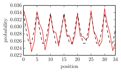
(a) $a=5$

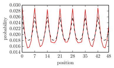
(b) $a=7$

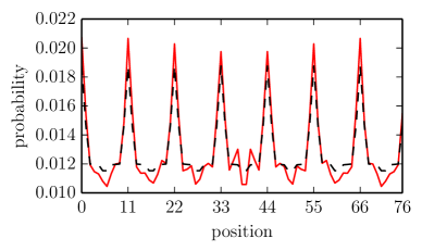
(c) $a=11$

Figure 3: Influence of one broken link on the time-averaged limiting probability distribution. Limiting distributions for the cases without broken link are plotted in black dotted line, whlist limiting distributions for the cases with one broken link are plotted in solid red line. The periodicity of the time-averaged limiting distribution is disturbed around the nodes without the connection. Here the broken link is located between nodes 18 and 19 (case 3(a)), 24 and 25 (case 3(b)), and 38 and 39 (case 3(c)), respectively and the initial state is of the form $\frac{1}{\sqrt{3}}(|0\rangle+|1\rangle+|2\rangle)\otimes|0\rangle$.

The second part of Eq. (27) can be interpreted as the laziness condition – e.g. in position $|0\rangle$ with coin pointing in the direction of a broken link, the walker does not move and the coin is changed from $|0\rangle$ to $|1\rangle$. However, one should note that due to the possibility of executing steps with a larger range, the cycle with broken links is not equivalent to a line segment.

The time-averaged limiting distribution in this situation is presented in Fig. 3. One can easily observe that the situation where one of the links is missing has a significant impact on the periodicity of the limiting distribution. The disturbance is particularly strong around the location of the broken link.

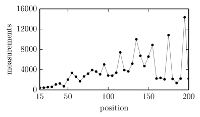
(a) $a=5$

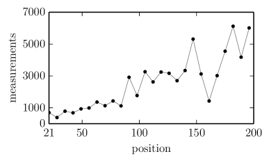
(b) $a=7$

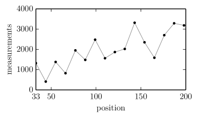
(c) $a=11$

Figure 4: Number of measurement required to assess if the network has one broken link. The plots represent results obtained for networks with number of nodes being a multiplicity of the liveliness parameter. Broken links are always between $\lfloor\frac{n}{2}\rfloor$ and $\lfloor\frac{n}{2}\rfloor+1$ nodes, where $n$ is number of nodes and the initial state is of the form$\frac{1}{\sqrt{3}}(|0\rangle+|1\rangle+|2\rangle)\otimes|0\rangle$.

Suppose we know the limiting distribution for the networks without and with a broken link, and denote them respectively $P_{0}$ and $P_{1}$. We want to asses if the given network has a broken link. In other words we need to make a statistical test which tells us if the considered model has distribution $P_{0}$ or $P_{1}$. Our goal is to estimate how many measurements are needed to discover one broken link and how this number depends on the size of the network.

This problem is equivalent to finding the relationship between the best ability to distinguish between statistical hypothesis ($H_{0}:\ P_{0}$ and $H_{1}:\ P_{1}$) and the size of a statistical sample (the number of measurements) [15]. The ability of distinguishing hypothesis is called the advantage and is expressed as

$$Adv_{q}(P_{0},P_{1})=|1-\alpha-\beta|,$$ (28)

where $q$ denotes a number of statistical samples, and $\alpha$ and $\beta$ are errors of type I and II, respectively. It turns out that there is a connection between the number of samples and the best advantage for distinguishing between distributions $P_{0}$ and $P_{1}$

$$1-BestAdv_{q}(P_{0},P_{1})\doteq 2^{-qC(P_{0},P_{1})},$$ (29)

where $\doteq$ denotes that two functions are asymptotically equivalent and $C(P_{0},P_{1})$ is called Chernoff information

$$C(P_{0},P_{1})=-\inf\limits_{0<\lambda<1}\log\sum\limits_{i}P_{0}(i)^{\lambda}P_{1}(i)^{1-\lambda}.$$ (30)

From Eq. (29) we obtain that if we have $q\approx\frac{1}{C(P_{0},P_{1})}$ samples, then we have the maximal ability to distinguish $P_{0}$ from $P_{1}$.

The number of measurements required in the case of lively quantum walk with one broken link is presented in Fig. 4. It is important to say, that results presented in Fig. 4 are obtained by numerical approximation of Chernoff information (30). One can observe that for large networks this number decreases with the growing liveliness parameter. This reflects the fact that the smaller networks and for the small liveliness parameter, the density of connections is higher. In such case one broken link does not have big impact on the network structure and, as the result, on the time-averaged limiting distribution. On the other hand, for larger networks and large liveliness parameter, the density of connections becomes smaller. This results in more significant impact of the broken connection on the observed behavior of the walk.

5 Concluding remarks

In this work we have introduced and studied a parametrized model of a quantum walk on cycle. The introduced model can be used to study the situation where the near-neighbor communication in the network is supplemented by the existence of the long-range links between the selected nodes.

The introduced model displays the periodicity of the time-averaged limiting distribution. We have proved that the periodicity of the limiting distribution is connected with the liveliness parameter.

The existence of additional connections enables the utilization of the introduced model for the purpose of quantum network exploration. In particular, the additional connection allows avoiding the trapping of the walker for any choice of the coin. This makes the lively walk resistant to the actions of a malicious party disturbing the programme of the quantum walker exploring the network.

Thanks to the introduction of additional connections, the lively walk can preserve its properties in the situation when one of the links is missing. This represents the situation when a structural error in the network occurs. We have shown that such errors disturb the periodicity properties of the introduced model. Moreover, one can argue that the additional connections can be beneficial from the point of view of quantum walk integrity. This is due to the fact that the additional connections make the network more resistant to broken links.

Acknowledgements

Work of PS has been supported by Polish National Science Centre under the research project 2013/11/N/ST6/03030, JAM has been supported by Ministry of Science and Higher Education under Iuventus Plus project IP 2014 031073 and MO has been supported by Polish National Science Centre under the research project 2011/03/D/ST6/00413.

Authors would like to thank Ł. Pawela and Z. Puchała for helpful suggestions and discussions during the preparation of the manuscript.

References

• [1] D. Reitzner, D. Nagaj, and V. Bužek. Quantum walks. Acta Phys. Slovaca, 61(6):603–725, 2012.
• [2] S.E. Venegas-Andraca. Quantum walks: a comprehensive review. Quantum Information Processing, 11(15):1015–1106, 2012.
• [3] R. Portugal. Quantum Walks and Search Algorithms. Springer-Verlag New York, U.S.A., 2013.
• [4] A. Ambainis. Quantum walks and their algorithmic applications. Int. J. Quant. Inf., 1:507–518, 2003.
• [5] C. Di Franco, M. McGettrick, and Th. Busch. Mimicking the probability distribution of a two-dimensional grover walk with a single-qubit coin. Phys. Rev. Lett., 106:080502, 2011.
• [6] M. Mc Gettrick and J.A. Miszczak. Quantum walks with memory on cycles. Physica A, 399:163–170, 2014. arXiv:1301.2905.
• [7] J.A. Miszczak and P. Sadowski. Quantum network exploration with a faulty sense of direction. Quantum Inform. Comput., 14(13&14), 2014. arXiv:1308.5923.
• [8] P. Sadowski. Efficient quantum search on Apollonian networks. arXiv:1406.0339.
• [9] Ł. Pawela, P. Gawron, J.A. Miszczak, and P. Sadowski. Generalized open quantum walks on Apollonian networks. PLoS ONE, 10(7):e0130967, 2015. arXiv:1407.1184.
• [10] R. Van Meter, T. Satoh, T.D. Ladd, W.J. Munro, and K. Nemoto. Path selection for quantum repeater networks. Networking Science, 3(1-4):82–95, 2013.
• [11] Ł. Pawela and J. Sładkowski. Cooperative quantum parrondo’s games. Physica D, 256:51–57, 2013. rXiv:1207.6954.
• [12] D. Aharonov, A. Ambainis, J. Kempe, and U. Vazirani. Quantum walks on graphs. In Proceedings of the 30th Annual ACM Symposium on Theory of Computation, pages 50–59. ACM Press, 2001.
• [13] M. Bednarska, A. Grudka, P. Kurzyński, T. Łuczak, and A. Wójcik. Quantum walks on cycles. Phys. Lett. A, 317(1-2):21–25, 2003.
• [14] E. Feldman, M. Hillery, H.-W. Lee, D. Reitzner, H. Zheng, and V. Bužek. Finding structural anomalies in graphs by means of quantum walks. Phys. Rev. A, 82(4):040301, 2010.
• [15] T. Baigneres and S. Vaudenay. The complexity of distinguishing distributions (invited talk). In Information Theoretic Security, pages 210–222. Springer, 2008.