Ground-state cooling of dispersively coupled optomechanical system in unresolved sideband regime via dissipatively coupled oscillator

Abstract

In the optomechanical cooling of a dispersively coupled oscillator, it is only possible to reach the oscillator ground state in the resolved sideband regime, where the cavity-mode line width is smaller than the resonant frequency of the mechanical oscillator being cooled. In this paper, we show that the dispersively coupled system can be cooled to the ground state in the unresolved sideband regime using an ancillary oscillator, which is coupled to the same optical mode via dissipative interaction. The ancillary oscillator has a resonant frequency close to that of the target oscillator; thus, the ancillary oscillator is also in the unresolved sideband regime. We require only a single blue-detuned laser mode to drive the cavity.

I Introduction

Quantum optomechanics studies the interactions between photons and mechanical oscillators. To facilitate applications yielding precise measurements and control features precise-1 ; precise-2 ; precise-3 ; precise-4 ; precise-5 ; precise-6 , certain quantum information processing techniques infor-1 ; infor-2 ; infor-3 ; infor-4 ; infor-5 , quantum foundations qc-1 ; qc-2 ; qc-3 , etc., it is necessary to prepare an oscillator in an almost pure state close to the zero-point vibration. Therefore, techniques for ground-state cooling that remedy the effects of stochastic driving from the thermal environment groundstate-1 ; groundstate-2 ; groundstate-3 ; GHz2 ; feedback-1 ; feedback-2 ; feedback-3 ; feedback-4 ; feedback-5 are fundamentally important opto-1 ; opto-2 ; review ; review-chen ; review-chinese . However, as regards attempts to realize the ground state of such an oscillator, even the $\textsuperscript{3}{\rm He}/\textsuperscript{4}{\rm He}$ dilution refrigerator is insufficient, unless the oscillator has very high resonant frequency (GHz) GHz1 ; GHz2 . Thus, it is necessary to exploit laser cooling schemes (or microwave techniques, etc., depending on the system).

Lasers are employed in optomechanical cooling in two ways review . One application is to measure the instant position of the oscillator. Then, an appropriate friction force is exerted in order to reduce the oscillation amplitude; this is known as cold damping quantum feedback feedback-1 ; feedback-2 ; feedback-3 ; feedback-4 ; feedback-5 , and the efficacy of this method depends on the measurement precision and the feedback loop quality limit-A . However, the second application is more interesting to us. It is based on that fact that, in some parameter regimes, the optomechanical interaction drives the cooling process automatically. The most extensively investigated interaction to generate this passive (or self-) cooling phenomenon is dispersive coupling, which is named for the feature in which the mechanical oscillator displacement changes the resonant frequency of the optical mode. Ground-state cooling involving such scenarios is valid only in the resolved sideband regime sideband-07-1 ; sideband-07-2 ; limit-A , where the mechanical resonant frequency is larger than the line width (or the damping rate) of the optical mode. Thus, this phenomenon is also referred to as sideband cooling.

From a practical perspective, an unresolved sideband regime allows one to use small drive detuning and, thus, small input power. Almost all the realized optomechanical systems with heavier oscillator functionality operate in the unresolved sideband regime review , and a well-known example is the suspended mirrors of the laser interferometer gravitational wave detector aligo . Therefore, eliminating the considerable limitation imposed by the requirement for a resolved sideband for ground-state cooling would enrich the optomechanical toolbox in a meaningful way.

Note that sideband resolution is not a stringent requirement in optomechanical systems with dissipative interaction, where the oscillator displacement changes the damping rate (or line width) of the optical mode diss-1 ; diss-X ; diss-expe ; diss-limit ; diss-realize ; diss-strong ; MS-ex ; new-1 ; new-2 . Although works on that topic are relatively rare, the predicted cooling has been verified experimentally MS-ex in an optomechanical system based on the Michelson-Sagnac interferometer diss-realize . Thus, the dissipative system is promising and merits further development. Here, we show that this system also sheds light on the dispersive system problem, i.e., ground-state cooling in the unresolved sideband regime.

In this study, we demonstrate that the dissipatively coupled oscillator in a hybrid optomechanical system comprised of both dispersively and dissipatively coupled oscillators cools not only itself, but also the dispersively coupled oscillator, which is coupled to the same cavity mode. Importantly, both of the oscillators are in the unresolved sideband regime. Thus, a solution to the difficult problem of cooling the dispersively coupled oscillator is provided. Note that this approach is not the first reported technique of this kind; however, the existing schemes for ground-state cooling in the unresolved sideband, such as cooling with optomechanically induced transparency (OMIT) eit-2 ; eit-cooling , coupled-cavity configurations mt-cav-2015 ; mt-cav-2014 , atom-optomechanical hybrid systems atom-2015 ; atom-1 ; atom-2 ; atom-3 ; atom-4 ; atom-5 ; atom-6 ; atom-7 , and the recently proposed scheme using quantum non-demolition interactions QND , require multiple driving lasers, multiple optical modes, high-quality cavities, and ground-state atom ensembles. Compared with those methods, our proposal offers a simpler option for cases in which dissipative coupling is accessible.

The remainder of this paper is organized as follows. In Sec. II, we briefly introduce the two kinds of optomechanical coupling and the quantum noise approach to the cooling limit. In Sec. III, we use the quantum noise approach to analyze the possibility of ground-state cooling in our system, which requires only one cavity mode and one laser driving mode. In Sec. IV, we use the exact solutions to the equations of motion to confirm the achievement of ground-state cooling in the unresolved sideband regime. In Sec. V, we discuss and compare the existing schemes and, in Sec. VI, we present the conclusion. Note that the natural unit $\hbar=1$ is used throughout this paper.

II Brief overview of passive cooling induced by quantum optical noise

Passive (or self-) cooling utilizes the optomechanical interaction to diminish the oscillation amplitude. The system investigated in this paper is illustrated in Fig. 1. It consists of two oscillators, with one being dispersively coupled and the other being dissipatively coupled to the same cavity mode. In this section, we introduce these two kinds of optomechanical coupling separately. The quantum noise approach to optomechanical cooling is emphasized and exploited in the next section in order to evidence the validity of our scheme.

II.1 Cooling with dispersive coupling

We first specify the definition of dispersive coupling. In a typical cavity optomechanics setup, the cavity end mirror plays the role of the oscillator. Displacement of this mirror alters the cavity length and, thus, the resonant frequency of the cavity mode; this leads to dispersive coupling, which can be described by the Hamiltonian

$$H_{int,0}=-g_{0}(\hat{b}_{0}+\hat{b}_{0}^{\dagger})(\hat{a}^{\dagger}\hat{a}-\langle\hat{a}^{\dagger}\hat{a}\rangle),$$ (1)

where $g_{0}$ is the coupling strength, $\hat{b}_{0}$ is the phonon annihilation operator, and $\hat{a}$ annihilates the cavity-mode photons. Hereafter, the suffix “0” will be reserved for this dispersively coupled oscillator.

In the expression for $H_{int,0}$, we have subtracted the steady-state photon number $\langle\hat{a}^{\dagger}\hat{a}\rangle=\alpha^{2}_{s}$, following the formulae of Ref. sideband-07-1 . It is assumed that $\alpha_{s}$ is a real number for convenience. This subtraction frees us from redefining parameters such as the cavity length and $\Delta$ (as in Ref. sideband-07-2 ), which are altered sightly because of the radiation pressure.

Suppose the cavity is driven by a single laser mode. The photons in the cavity strive to reach a frequency close to resonance. Therefore, if the input laser (with frequency $\omega_{d}$) is red detuned to the cavity mode ($\omega_{c}$), which corresponds to the detuning $\Delta=\omega_{d}-\omega_{c}<0$, the input photons preferentially extract energy from the oscillator via the interaction described by Eq. (1). This mechanism constitutes a simple explanation of dispersive cooling, from which we can further infer that the optimal detuning is $\Delta=-\omega_{0}$ (the resonant frequency of the oscillator) in the weak coupling regime.

It is convention to refer to the energy quanta of the mechanical oscillator as phonons. Then, the Fermi golden rule indicates that, for the oscillator, the optics-induced emission or absorption of phonons occurs at a rate that depends on the the photon-number fluctuation spectrum at $\omega=\pm\omega_{0}$. This spectrum is given by

$$S^{0}_{nn}[\omega] =\int_{-\infty}^{\infty}d\tau e^{i\omega\tau}\langle\delta\hat{n}(\tau)\delta\hat{n}(0)\rangle,$$ (2)

$$=\frac{\kappa\alpha_{s}^{2}}{\kappa^{2}/4+(\omega+\Delta)^{2}},$$

where $\delta\hat{n}=\hat{a}^{\dagger}\hat{a}-\langle\hat{a}^{\dagger}\hat{a}\rangle$ and $\kappa$ is the line-width of the cavity mode in question. The damping rate induced by the optics is then

$$\gamma_{opt,0}=g_{0}^{2}(S_{nn}^{0}[\omega_{0}]-S^{0}_{nn}[-\omega_{0}]).$$ (3)

The balance between the optics-induced emission and absorption leads to a steady-state phonon occupation (when $\Delta<0$)

$$n_{opt,0}= \frac{S^{0}_{nn}[-\omega_{0}]}{S^{0}_{nn}[\omega_{0}]-S^{0}_{nn}[-\omega_{0}]},$$ (4)

$$= -\frac{(\omega_{0}+\Delta)^{2}+\kappa^{2}/4}{4\omega_{0}\Delta}.$$

Incorporating the influence of the thermal environment, the full expression of the phonon number is

$$\tilde{n}_{0}=\frac{\gamma_{opt,0}n_{opt,0}+\gamma_{0}n_{th,0}}{\gamma_{opt,0}+\gamma_{0}},$$ (5)

where $\gamma_{0}$ and $n_{th,0}$ represent the damping rate and the phonon occupation in the absence of the optical system, respectively.

Equation (5) implies that ground-state cooling occurs if $\gamma_{opt,0}\gg\gamma_{0}$ and $n_{opt,0}\ll 1$. In the resolved sideband regime, where $\omega_{0}>\kappa$, $n_{opt,0}$ reaches its minimum $(\frac{\kappa}{4\omega_{0}})^{2}$ when $\Delta=-\omega_{0}$. Ground-state cooling is, therefore, possible in this regime. In contrast, in the unresolved sideband regime, where $\kappa\gg\omega_{0}$, the minimum of $n_{opt,0}$ is $\frac{\kappa}{4\omega_{0}}$, for which the detuning should be $\Delta=-\kappa/2$. Obviously, it is difficult for $n_{opt}$ to be close to zero, and this leads to problematic cooling of the dispersive optomechanical system in the unresolved sideband regime.

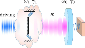
Figure 1: Hybrid optomechanical system of dispersively and dissipatively coupled oscillators. The oscillators are coupled to the same cavity mode, with line width $\kappa$. This mode is driven by one laser mode only, with blue detuning $\Delta>0$.

II.2 Cooling with dissipative coupling

If the displacement of the oscillator modifies $\kappa$, the induced coupling is called dissipative. Dissipative coupling was first proposed in Ref. diss-1 and then experimentally implemented in a nanomechanical system diss-expe ; diss-X . Reference diss-realize gave another experimental construction involving the Michelson-Sagnac interferometer, which was implemented in experiment very recently MS-ex . The strong coupling effects diss-strong , cooling limit diss-limit , anomalous dynamic backactions new-1 , and stabilities new-2 associated with dissipative cooling have also been studied recently. However, research on this topic is rare in comparison with the literature on dispersive optomechanics.

Throughout this paper, terms related to the dissipatively coupled oscillator are marked by the subscript “1”. The dissipative coupling is described by the Hamiltonian

$$H_{int,1}=-ig_{1}\sqrt{\frac{\kappa}{2\pi\rho}}\sum_{q}(\hat{a}^{\dagger}\hat{b}_{q}-\hat{b}^{\dagger}_{q}\hat{a})(\hat{b}^{\dagger}_{1}+\hat{b}_{1}),$$ (6)

where the summation is taken over the environment modes $\hat{b}_{q}$, the density of states of which is assumed to be a constant $\rho$.

The cooling mechanism is less transparent than in the dispersive case. Following the quantum noise approach, the force spectrum responsible for the optomechanical cooling is

$$S_{FF}[\omega]=\kappa g_{1}^{2}\alpha_{s}^{2}\frac{(\omega+2\Delta)^{2}}{\kappa^{2}/4+(\omega+\Delta)^{2}}.$$ (7)

The rate of phonon generation is $S_{FF}[-\omega_{1}]$ and that of phonon loss is $S_{FF}[\omega_{1}]$. The optically induced damping rate is, therefore, given by their difference

$$\gamma_{opt,1}=S_{FF}[\omega_{1}]-S_{FF}[-\omega_{1}].$$ (8)

The further formulas for $n_{opt,1}$ and the final phonon number $\tilde{n}_{1}$ are in the same forms as Eqs. (4) and (5).

Despite the sideband resolution, both $S_{FF}[-\omega_{1}]$ and $n_{opt,1}$ vanish if the driving laser is blue detuned at $\Delta=\omega_{1}/2$. The conclusion can then be drawn that ground-state cooling is robust, provided a high mechanical quality factor and proper pre-cooling is supplied. This point is verified by the numerical calculations given in diss-1 ; diss-strong , which show that $\tilde{n}_{1}$ can be reduced to the level of $10^{-2}$ from the initial occupation $n_{th,1}=100$.

III Ground-state cooling: Evidence from quantum noise approach

In this section, we use the quantum noise approach to show that the dispersively coupled oscillator can be cooled to the ground state with the assistance of a dissipative oscillator. Both of these oscillators are in the unresolved sideband regime. As previously, the quantities of the target dispersive oscillator are marked with subscript “0”, and those of the ancillary dissipative oscillator are indicated by subscript “1”.

III.1 Model and equations

In the frame of the driving laser, the Hamiltonian of the entire system is

$$H= -\Delta(\hat{a}^{\dagger}\hat{a}-\langle\hat{a}^{\dagger}\hat{a}\rangle)+\omega_{0}\hat{b}_{0}^{\dagger}\hat{b}_{0}+\omega_{1}\hat{b}_{1}^{\dagger}\hat{b}_{1}$$ (9)

$$+H_{int,0}+H_{int,1}+H_{\kappa}+H_{\gamma_{0}}+H_{\gamma_{1}},$$

where $H_{\gamma_{0}}$ and $H_{\gamma_{1}}$ are the thermal damping terms of the two oscillators. Further,

$$H_{\kappa}=-i\sqrt{\frac{\kappa}{2\pi\rho}}\sum_{q}(\hat{a}^{\dagger}\hat{b}_{q}-\hat{b}^{\dagger}_{q}\hat{a}),$$ (10)

describes the damping of the cavity mode induced by the environment, including the driving mode. The free Hamiltonian of the environment modes is not presented explicitly.

To derive the equations of motion, the input-output formalism review-noise is considered, which yields

$$\sqrt{\frac{\kappa}{2\pi\rho}}\sum_{q}\hat{b}_{q}=\sqrt{\kappa}\hat{a}_{in}+\frac{\kappa}{2}\hat{a}+g_{1}\frac{\kappa}{2}(\hat{b}_{1}+\hat{b}^{\dagger}_{1})\hat{a}.$$ (11)

This formula can be used to obtain the quantum Langevin equations and, also, to further linearize them by separating the operators associated with optics into steady-state and quantum-fluctuation components. That is, we assume that $\alpha_{s}$ is sufficiently significant that $\hat{a}_{in}=\bar{a}_{in}+\hat{d}_{in}$ and $\hat{a}=\alpha_{s}+\hat{d}$. The two steady-state average amplitudes are correlated by $(i\Delta-\kappa/2)\alpha_{s}=\sqrt{\kappa}\bar{a}_{in}$.

After the linearizion, the quantum Langevin equations of the cavity mode and the mechanical oscillators are expressed as

$$\dot{\hat{d}} = (i\Delta-\frac{\kappa}{2})\hat{d}-\sqrt{\kappa}\hat{d}_{in}+ig_{0}\alpha_{s}(\hat{b}_{0}+\hat{b}_{0}^{\dagger})$$ (12)

$$-g_{1}\alpha_{s}(i\Delta+\frac{\kappa}{2})(\hat{b}_{1}+\hat{b}_{1}^{\dagger}),$$

$$\dot{\hat{b}}_{0} = -(i\omega_{0}+\frac{\gamma_{0}}{2})\hat{b}_{0}-\sqrt{\gamma_{0}}\hat{b}_{in,0}+ig_{0}\alpha_{s}(\hat{d}+\hat{d}^{\dagger}),$$ (13)

$$\dot{\hat{b}}_{1} = -(i\omega_{1}+\frac{\gamma_{1}}{2})\hat{b}_{1}-\sqrt{\gamma_{1}}\hat{b}_{in,1}-g_{1}\alpha_{s}\sqrt{\kappa}(\hat{d}_{in}-\hat{d}_{in}^{\dagger})$$ (14)

$$-ig_{1}\alpha_{s}\Delta(\hat{d}+\hat{d}^{\dagger})-g_{1}\alpha_{s}\frac{\kappa}{2}(\hat{d}-\hat{d}^{\dagger}).$$

In those equations, the noise terms with subscript “in” satisfy the correlations

$$\langle\hat{d}_{in}(t)\hat{d}^{\dagger}_{in}(t^{\prime})\rangle =\delta(t-t^{\prime}),$$ (15)

$$\langle\hat{b}_{in,k}(t)\hat{b}^{\dagger}_{in,k}(t^{\prime})\rangle =(n_{th,k}+1)\delta(t-t^{\prime}),$$

$$\langle\hat{b}^{\dagger}_{in,k}(t)\hat{b}_{in,k}(t^{\prime})\rangle =n_{th,k}\delta(t-t^{\prime}),$$

where $n_{th,k}$ is the thermal equilibrium phonon number of oscillator $k$ (where $k=0,1$). All other two-operator correlation functions vanish.

We can include the conjugate equations and write the complete set of equations in the form $\frac{d}{dt}\vec{V}=M\cdot\vec{V}+\vec{V}_{in}$, where $\vec{V}=(\hat{d},\hat{d}^{\dagger},\hat{b}_{0},\hat{b}_{0}^{\dagger},\hat{b}_{1},\hat{b}_{1}^{\dagger})$ and $\vec{V}_{in}$ has a similar definition. The system is dynamically stable if the eigenvalues of the matrix $M$ have no negative real parts, which can be easily checked after the parameters are fixed. We find that the issue of stability forbids $\Delta=-\omega_{1}$ in the unresolved sideband regime when $\kappa\gg\omega_{1}$, while this detuning allows ground-state cooling when $\kappa$ and $\omega_{1}$ are comparable or in the resolved sideband regime diss-1 ; diss-strong .

III.2 Photon-number fluctuation spectrum

In Sec. II.1, it was shown that the photon-number fluctuation spectrum is responsible for the cooling of oscillator 0. To calculate this spectrum, we follow the strategy used in Ref. eit-cooling , i.e., we ignore the backaction of oscillator 0 to the optical field but consider that of oscillator 1. Note that the validity of this strategy is examined in Sec. IV via a numerical calculation of the cooling limit from the linearized Langevin equations.

Applying Fourier transformations to Eqs. (12) and (14) with $g_{0}=0$, we obtain a series of algebraic equations that are exactly solvable. The Fourier transformation is conducted with the conventions

$$\hat{f}_{\omega}=\int_{-\infty}^{\infty}dte^{i\omega t}\hat{f}(t),$$ (16)

and $\hat{f}^{\dagger}_{\omega}\equiv(\hat{f}^{\dagger})_{\omega}=(\hat{f}_{-\omega})^{\dagger}$. The photon number fluctuation annihilation operator $\hat{d}(t)$ is transformed to

$$\hat{d}_{\omega}=-\sqrt{\kappa}\chi_{c,\omega}\hat{d}_{in,\omega}-g_{1}\alpha_{s}(i\Delta+\frac{\kappa}{2})\chi_{c,\omega}\hat{x}_{1,\omega},$$ (17)

where $\hat{x}_{1,\omega}=\hat{b}_{1,\omega}+\hat{b}_{1,\omega}^{\dagger}$ and

$$\hat{b}_{1,\omega}= -\frac{\sqrt{\gamma_{1}}}{N[\omega]}\{\chi_{1,-\omega}^{*-1}\hat{b}_{in,1,\omega}-i\Sigma[\omega](\hat{b}_{in,1,\omega}+\hat{b}_{in,1,\omega}^{\dagger})\}$$ (18)

$$-g_{1}\alpha_{s}\frac{\sqrt{\kappa}}{N[\omega]}\chi^{*-1}_{1,-\omega}[\alpha(\omega)\hat{d}_{in,\omega}-\alpha^{*}(-\omega)\hat{d}^{\dagger}_{in,\omega}].$$

In the above equations, the susceptibilities of the optical mode $\chi_{c}$ and oscillator 1 $\chi_{1}$ are defined as

$$\chi^{-1}_{c,\omega} = \kappa/2-i(\omega+\Delta),$$ (19)

$$\chi^{-1}_{1,\omega} = \gamma_{1}/2-i(\omega-\omega_{1}),$$ (20)

and the other quantities are

$$\alpha(\omega) = 1-\chi_{c,\omega}(i\Delta+\kappa/2),$$ (21)

$$N[\omega] = \chi^{-1}_{1,\omega}\chi^{*-1}_{1,-\omega}+2\omega_{1}\Sigma[\omega],$$ (22)

with the “self-energy” term

$$\Sigma[\omega]=ig_{1}^{2}\alpha_{s}^{2}\left\{\chi_{c,\omega}\left(i\Delta+\frac{\kappa}{2}\right)^{2}-\chi^{*}_{c,-\omega}\left(i\Delta-\frac{\kappa}{2}\right)^{2}\right\}.$$ (23)

Next, we proceed to examine the photon-number fluctuation spectrum. As $\delta\hat{n}=\alpha_{s}(\hat{d}+\hat{d}^{\dagger})$ and

$$\hat{d}_{\omega}+\hat{d}^{\dagger}_{\omega}= -\sqrt{\kappa}(\chi_{c,\omega}\hat{d}_{in,\omega}+\chi^{*}_{c,-\omega}\hat{d}^{\dagger}_{in,\omega})$$ (24)

$$-g_{1}\alpha_{s}A(\omega)\hat{x}_{1,\omega},$$

where $A(\omega)=\chi_{c,\omega}(i\Delta+\kappa/2)+\chi^{*}_{c,-\omega}(-i\Delta+\kappa/2)$, the fluctuation spectrum can be expressed as

$$S_{nn}[\omega]= S_{nn}^{0}[\omega]+g_{1}^{2}\alpha_{s}^{4}|A(\omega)|^{2}S^{1}_{xx}[\omega]$$ (25)

$$+\sqrt{\kappa}g_{1}\alpha_{s}^{3}\{A(-\omega)S_{cx}[\omega]+A(\omega)S_{xc}[\omega]\}.$$

Therein, $S_{nn}^{0}$ is the bare spectrum given in Eq. (2) and $S_{xx}^{1}[\omega]$ is the spectrum of the position of oscillator 1

$$S_{xx}^{1}[\omega]=\int_{-\infty}^{\infty}\frac{d\omega^{\prime}}{2\pi}\langle\hat{x}_{1,\omega}\hat{x}_{1,\omega^{\prime}}\rangle.$$ (26)

$S_{cx}[\omega]$ is the correlation between oscillator 1 and the $X$-quadrature of the optical mode in the absence of oscillator 1, such that

$$S_{cx}[\omega]=\int_{-\infty}^{\infty}\frac{d\omega^{\prime}}{2\pi}\langle\hat{M}_{c}[\omega]\hat{x}_{1,\omega^{\prime}}\rangle,$$ (27)

where $\hat{M}_{c}[\omega]=\chi_{c,\omega}\hat{d}_{in,\omega}+\chi^{*}_{c,-\omega}\hat{d}^{\dagger}_{in,\omega}$. $S_{xc}$ is defined similarly.

III.3 Ground-state cooling

We know that, in the unresolved sideband regime, the gap between $S^{0}_{nn}[\pm\omega_{0}]$ is too narrow to support ground-state cooling. Now, the photon number fluctuation spectrum [Eq. (25)] contains two more terms than the bare $S^{0}_{nn}$. Thus, we examine the manner in which these additional terms unbalance the spectrum. For this purpose, the exact expressions presented in the previous subsection are not sufficiently transparent for the result to be observed. Therefore, we further simply them by assuming weak coupling.

III.3.1 $S_{nn}[\omega]$ shape

When oscillator 1 is decoupled to the optical field, its position-position correlation spectrum is expressed in terms of the “bare” damping rate $\gamma_{1}$, resonant frequency (incorporated in the susceptibility $\chi_{1,\omega}$), and thermal equilibrium phonon occupation $n_{th,1}$:

$$\gamma_{1}\{|\chi_{1,\omega}|^{2}(n_{th,1}+1)+|\chi_{1,-\omega}|^{2}n_{th,1}\}.$$

When the opto-mechanical coupling is weak, the effective damping rate $\tilde{\gamma}_{1}$, resonant frequency $\tilde{\omega}_{1}$, and phonon occupation $\tilde{n}_{1}$ can be well defined. By replacing the bare terms with the effective terms, $\chi_{1,\omega}$ is modified to

$$\tilde{\chi}_{1,\omega}=\frac{1}{\tilde{\gamma}_{1}/2-i(\omega-\tilde{\omega}_{1})},$$ (28)

where $\tilde{\gamma}_{1}=\gamma_{1}+\gamma_{opt,1}$. Further,

$$\tilde{\omega}_{1} = \omega_{1}+\Re(\Sigma[\omega_{1}])\approx\omega_{1}-6g_{1}^{2}\alpha_{s}^{2}\Delta,$$ (29)

$$\tilde{\gamma}_{1} = \gamma_{1}-2\Im(\Sigma[\omega_{1}])\approx\gamma_{1}+16g_{1}^{2}\alpha_{s}^{2}\Delta^{2}/\kappa,$$ (30)

where $\Re$ and $\Im$ represent the real and imaginary parts, respectively. The approximations on the right hand side are conducted in the unresolved sideband regime, with the additional assumption that $\Delta$ has the same scale as $\omega_{0/1}$. Additionally, for Eq. (29), a superior approximation is

$$\tilde{\omega}_{1}=\sqrt{\omega_{1}^{2}+2\omega_{1}\Re(\Sigma[\omega_{1}])}.$$ (31)

The $\tilde{n}_{1}$ in Eq. (28) corresponds to the phonon number obtained in the dissipative optomechanical system. As discussed in Sec. II.2, this can be very close to zero when $\Delta=\omega_{1}/2$.

Finally, the position spectrum is expressed as

$$S^{1}_{xx}[\omega]=\tilde{\gamma}_{1}\{|\tilde{\chi}_{1,\omega}|^{2}(\tilde{n}_{1}+1)+|\tilde{\chi}_{1,-\omega}|^{2}\tilde{n}_{1}\},$$ (32)

where $\tilde{n}_{1}$ is the phonon occupation after the optomechanical cooling. As explained in Sec. II.2, $\tilde{n}_{1}$ approaches zero if $\Delta$ is properly adjusted. The interference terms between the displacement of oscillator 1 and the optics field are expressed as

$$S_{cx}[\omega]=-i2\omega_{1}g_{1}\alpha_{s}\frac{\sqrt{\kappa}}{N[-\omega]}\chi_{c,\omega}\alpha^{*}(\omega),$$ (33)

$$S_{xc}[\omega]=i2\omega_{1}g_{1}\alpha_{s}\frac{\sqrt{\kappa}}{N[\omega]}\chi^{*}_{c,\omega}\alpha(\omega).$$

Note that the two interference terms are complex conjugate, as $N[\omega]=N^{*}[-\omega]$. In particular, we can approximate $N[\omega]\approx\tilde{\chi}^{-1}_{1,\omega}\tilde{\chi}^{*-1}_{1,-\omega}$.

Next, let us examine the shape of $S_{xx}^{1}[\omega]$. Equation (32) indicates that there are two peaks at $\omega=\pm\tilde{\omega}_{1}$. The ratio of their heights is $1+1/\tilde{n}_{1}$, which implies an extreme asymmetry in the limit $\tilde{n}_{1}\rightarrow 0$. We wish to investigate whether or not this asymmetry can meet our requirements for ground-state cooling.

III.3.2 Cooling: Near the limit $\omega_{0}=\tilde{\omega}_{1}$

If $|\omega_{0}-\tilde{\omega}_{1}|<\tilde{\gamma}_{1}$, $\pm\omega_{0}$ is located in the peak range. We focus on the limit case at resonance in what follows, i.e., where $\omega_{0}=\tilde{\omega}_{1}$ or, more loosely, $|\omega_{0}-\tilde{\omega}_{1}|\ll\tilde{\gamma}_{1}$. Other possibilities are studied in the next subsection.

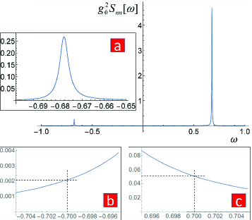
Figure 2: Photon-number fluctuation spectrum $g_{0}^{2}S_{nn}[\omega]$. $\omega_{1}$ is set as the unit, which means $\omega_{1}=1$. The other parameters are: $\kappa=300$, $\gamma_{1}=10^{-6}$, $g_{0}\alpha_{s}=0.1$, $g_{1}\alpha_{s}=0.3$, $n_{1,th}=100$, and $\Delta=0.5$. The peaks are located at $\pm\tilde{\omega}_{1}\approx\pm 0.678$. The left peak is significantly shorter than the right. (a) Magnification of $-\tilde{\omega}_{1}\approx-0.678$ peak. If $\omega_{0}=\tilde{\omega}_{1}$, $n_{0,opt}\approx 0.061$. (b, c) If $\pm\omega_{0}$ is located away from the peaks, say at $\pm 0.7$, then $g_{0}^{2}S_{nn}[\omega_{0}]=0.051$ and $g_{0}^{2}S_{nn}[-\omega_{0}]=0.0021$, such that $n_{0,opt}\approx 0.042$.

In the unresolved sideband regime and the considered case when $\omega$ is close to $\pm\omega_{0}$, we have the approximations

$$\alpha(\omega)\approx\frac{\omega+2\Delta}{i\kappa/2},\qquad A(\omega)\approx 2-i\frac{4\omega}{\kappa},$$ (34)

$$\chi_{1,\omega_{0}}=\frac{2}{\tilde{\gamma_{1}}},\qquad\chi_{c,\omega}\approx\frac{2}{\kappa}(1+\frac{2i(\omega+\Delta)}{\kappa}).$$

We also assume that the mechanical oscillators have high quality factors and that $\tilde{\gamma}_{1}\ll\tilde{\omega}_{1}$. For convenience in what follows, we introduce a factor $\beta$ such that $\omega_{0}+\tilde{\omega}_{1}=\beta^{-1}\omega_{1}$. In fact, $\beta$ should be slightly larger than $1/2$. Then, in $S_{cx}$ and $S_{xc}$, we have

$$\frac{\omega_{1}}{N[\omega]}= i\beta\tilde{\chi}_{1,\omega}, \omega\sim\omega_{0}$$ , (35)

$$\frac{\omega_{1}}{N[\omega]}= -i\beta\tilde{\chi}^{*}_{1,-\omega}, \omega\sim-\omega_{0}$$ . (36)

Following these preparations, the fluctuation spectrum at $\pm\omega_{0}$ can be expressed approximately as

$$S_{nn}[\omega_{0}] = S_{nn}^{0}[\omega_{0}]+4g_{1}^{2}\alpha_{s}^{4}\tilde{\gamma}_{1}\left[\frac{4}{\tilde{\gamma}_{1}^{2}}(\tilde{n}_{1}+1)+\frac{\beta^{2}}{\omega_{1}^{2}}\tilde{n}_{1}\right]$$ (37)

$$+128g_{1}^{2}\alpha_{s}^{4}\beta\frac{(\Delta+2\omega_{0})(\omega_{0}+2\Delta)}{\kappa^{2}\tilde{\gamma}_{1}},$$

$$S_{nn}[-\omega_{0}] = S_{nn}^{0}[-\omega_{0}]+4g_{1}^{2}\alpha_{s}^{4}\tilde{\gamma}_{1}\left[\frac{4}{\tilde{\gamma}_{1}^{2}}\tilde{n}_{1}+\frac{\beta^{2}}{\omega_{1}^{2}}(\tilde{n}_{1}+1)\right]$$ (38)

$$-128g_{1}^{2}\alpha_{s}^{4}\beta\frac{(\Delta-2\omega_{0})(2\Delta-\omega_{0})}{\kappa^{2}\tilde{\gamma}_{1}},$$

Here, the conditions $\kappa\gg\omega_{0}\gg\tilde{\gamma}_{1}\gg\gamma_{1}$ and $\tilde{\gamma}_{1}\kappa\sim\omega_{1}^{2}$, which is supported by Eq. (30), are adopted. Then, the steady-state phonon number $n_{opt,0}$ is

$$n_{opt,0}\approx\tilde{n}_{1}+O(\frac{\omega_{0}^{2}}{\kappa^{2}})+O(\frac{\tilde{\gamma}_{1}^{2}}{4\omega_{1}^{2}}).$$ (39)

In the above equation, we have neglected terms of $O(\tilde{n}_{1}/\kappa^{2})$ or higher. Therefore, roughly speaking, $n_{opt,0}$ equates to $\tilde{n}_{1}$. As the ancillary oscillator can be cooled to near the ground state when $\Delta=\omega_{1}/2$, ground-state cooling of the dispersively coupled oscillator 1 is indicated.

Figure 2 clearly illustrates the asymmetrical feature of $S_{nn}[\omega]$. The parameters are listed in the caption. With those parameters, the standard sideband cooling with the optimal setting $\Delta=-\kappa/2$ yields $n_{opt,0}\approx 110.6>n_{th,0}=100$. Beginning at this limit, the ancillary oscillator helps to unbalance the $S_{nn}[\omega]$ peaks and implies a new limit at ${n}_{opt,0}=0.061$.

III.3.3 Cooling: Off the peaks

In this subsection, we release the restriction that $|\omega_{0}-\tilde{\omega}_{1}|<\tilde{\gamma}_{1}$. However, the preliminary requirement that the $\pm\omega_{0}$ are not far from the peaks is retained. (Otherwise, the incorporation of oscillator 1 becomes meaningless.)

Now, the imbalance is no longer manifest from the shape of $S_{nn}[\omega]$ and a detailed calculation is necessary. To specify the conditions of this discussion, we assume that $\tilde{\gamma}_{1}\ll|\omega_{0}-\tilde{\omega}_{1}|\ll\omega_{0}+\tilde{\omega}_{1}$ and $\Delta$ is on the scale of $\omega_{0/1}$. Hence, the approximations in Eq. (34) remain valid, apart from the effective susceptibility of oscillator 1, which should be altered to

$$\tilde{\chi}_{1,\pm\omega_{0}}\approx\frac{i}{\pm\omega_{0}-\tilde{\omega}_{1}}.$$ (40)

We do not give the expressions of the phonon-number fluctuation spectrum at $\pm\omega_{0}$ explicitly here. In fact, all the terms exactly or approximately have a factor $1/\kappa$. However, among them, the dominant terms of $O[(\frac{\omega_{0}}{\omega_{0}-\tilde{\omega}_{1}})^{2}]$ are

$$S_{nn}[\omega_{0}] \approx 4g_{1}^{2}\alpha_{s}^{4}\tilde{\gamma}_{1}\frac{\tilde{n}_{1}+1}{(\omega_{0}-\tilde{\omega}_{1})^{2}},$$

$$S_{nn}[-\omega_{0}] \approx 4g_{1}^{2}\alpha_{s}^{4}\tilde{\gamma}_{1}\frac{\tilde{n}_{1}}{(\omega_{0}-\tilde{\omega}_{1})^{2}}.$$ (41)

Besides the considerable value of $g_{1}\alpha_{s}$ and the condition that $\frac{\omega_{0/1}}{|\omega_{0}-\tilde{\omega}_{1}|}\gg 1$, the validity of the above approximations also relies on the preliminary that $\frac{\tilde{n}_{1}}{(\omega_{0}-\tilde{\omega}_{1})^{2}}$ covers $\frac{1}{(\omega_{0}+\tilde{\omega}_{1})^{2}}$. Then, we have

$$\gamma_{opt,0}=4g_{0}^{2}g_{1}^{2}\alpha_{s}^{4}\frac{\tilde{\gamma}_{1}}{(\omega_{0}-\tilde{\omega}_{1})^{2}},\qquad n_{opt,0}\approx\tilde{n}_{1}.$$ (42)

Therefore, building on the conditions that support Eq. (42), the dispersively coupled oscillator can be cooled to the ground state.

In Fig. 2, the roots of the left and right peaks are magnified and their height imbalance is shown. A cooling limit at $n_{opt,0}=0.042$ is predicted.

III.4 Fixing the experimental parameters

From the above analysis, it seems that the optimal detuning is $\omega_{1}/2$, because this value yields the minimal $\tilde{n}_{1}$. However, this intuition is not exactly correct. Here, we inspect the cooling mechanism more closely and study the parameters of the experimental variables that most strongly benefit cooling via this quantum noise approach.

III.4.1 Sources contributing to $S_{nn}[\pm\omega_{0}]$

The photon-number fluctuation spectrum is calculated from the $X$-quadrature $d_{\omega}+d^{\dagger}_{\omega}$, which can be rewritten according to the independent contributing sources as

$$-\sqrt{\kappa}\left\{\chi_{c,\omega}+i\frac{2\omega_{1}g_{1}^{2}\alpha_{s}^{2}\alpha(\omega)A(\omega)}{N[\omega]}\right\}\hat{d}_{in,\omega}$$ (43)

$$\qquad+g_{1}\alpha_{s}\sqrt{\gamma_{1}}\frac{A(\omega)}{N[\omega]}\chi^{*-1}_{1,-\omega}\hat{b}_{1,in,\omega}+h.c.,$$

where $h.c.$ represents the hermitian conjugate, followed by the transformation $\omega\rightarrow-\omega$. We remind readers that $A(\omega)=A^{*}(-\omega)$ and $N[\omega]=N^{*}[-\omega]$.

In Eq. (43), the second line is due to the thermal environment of oscillator 1. Using Eq. (15), it is apparent that, when $n_{1,th}\gg 1$, the thermal noise contributes to $S_{nn}[\pm\omega]$ equally (see the blue dashed lines in Fig. 3) with the value

$$\qquad g_{0}^{2}g_{1}^{2}\alpha_{s}^{4}\gamma_{1}|\frac{A(\omega)}{N[\omega]}|^{2}(|\chi^{-1}_{1,\omega}|^{2}+|\chi^{-1}_{1,-\omega}|^{2})n_{1,th}.$$ (44)

This implies that the imbalance in $S_{nn}[\omega]$ should be attributed to the terms in the first line of Eq. (43), i.e., those from the optical field.

The optical contribution component is interference between that filtered by the cavity (represented by $\chi_{c,\omega}$) and that introduced by oscillator 1 (represented by the $g_{1}$ factor). Note that, for the former in the unresolved sideband regime, we have $\chi_{c,\omega}\approx 2/\kappa$, which is a small constant that affects both peaks equally. Thus, the prospect of cooling is dependent on the latter. This contribution must outweigh Eq. (44) by a large extent at $\omega=\omega_{0}$, and take advantage of the destructive interference at $\omega=-\omega_{0}$. Otherwise, the $S_{nn}[\omega]$ imbalance necessary for ground-state cooling cannot be established.

III.4.2 Mechanical quality factor

To achieve ground-state cooling, the contribution to $S_{nn}[\omega_{0}]$ from the first line of Eq. (43) must be significantly larger than that given in Eq. (44). The ratio is

$$\frac{\omega_{1}/\gamma_{1}}{\kappa/\omega_{1}}\frac{16g_{1}^{2}\alpha_{s}^{2}(\omega+2\Delta)^{2}}{n_{th,1}(|\chi_{1,\omega}^{-1}|^{2}+|\chi_{1,-\omega}^{-1}|)},$$ (45)

where we have approximated $\alpha(\omega)$ according to Eq. (34). As $\Delta$ is chosen to be of the same scale as $\omega_{0/1}$, the value of the ratio depends on the first factor, i.e., the quality factor of oscillator 1, $\omega_{1}/\gamma_{1}$, vs. the sideband parameter $\kappa/\omega_{1}$. Because of our unresolved sideband regime preliminary, Eq. (45) demonstrates the requirement for a high mechanical quality factor, which is selected as $10^{6}$ in Fig. 3. Otherwise, we cannot obtain a small value for $n_{0,opt}$, which is necessary for ground-state cooling.

When $\kappa/\omega_{1}$ and $\omega_{1}/\gamma_{1}$ are fixed, Eq. (45) also provides indications of the requirements for pre-cooling (which determines $n_{1,th}$) and the effective coupling strength $g_{1}\alpha_{s}$. Meanwhile, the value of $\omega_{0}+2\Delta$ in the Eq. (45) denominator cannot be too small.

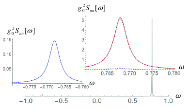
Figure 3: $g_{0}^{2}S_{nn}[\omega]$ when $\Delta=\omega_{0}/2$. We set $\omega_{1}$ as the unit, which means $\omega_{1}=1$. The other experimental parameters are: $\kappa=300$ and $\gamma_{1}=10^{-6}$ (such that the quality factor of oscillator 1 is $10^{6}$), $g_{0}\alpha_{s}=0.1$, $g_{1}\alpha_{s}=0.3$, $n_{1,th}=100$, $\omega_{0}=0.76$, and $\Delta=0.38$. The peaks are located at $\pm\tilde{\omega}_{1}\approx\pm 0.768$. The peaks are presented separately. The red and blue dashed lines indicate the contributions from the optical field noise and the thermal environment of oscillator 1, respectively. $S_{nn}[\omega_{0}]=0.2814$ and $S_{nn}[-\omega_{0}]=0.0076$, such that $n_{0,opt}\approx 0.0277$.

III.4.3 Selection of optimal detuning

The factor $1/N[\omega]$ is absent from Eq. (45), but must be taken into account when comparing the scales of the two terms in the first line of Eq. (43). $N[\omega_{0}]$ of small magnitude could significantly enhance the value of $S_{nn}[\omega_{0}]$, and also result in a large $\gamma_{opt,0}$. The remaining term $\chi_{c,\omega}$ is sufficiently small in magnitude to be neglected. From Eq. (34), it is apparent that

$$|N[\omega]|=|\omega_{0}^{2}-\tilde{\omega}_{1}^{2}|,$$ (46)

near $\omega=\pm\omega_{0}$. Thus, the condition $|\omega_{0}-\tilde{\omega}_{1}|\ll\omega_{0/1}$ proposed in the previous section is satisfied. According to Eq. (29), $\omega_{1}-\tilde{\omega}_{1}\approx 6g_{1}^{2}\alpha_{s}^{2}\Delta$. Therefore, in the optimal cooling region, $g_{1}\alpha_{s}$ and $\Delta$ exhibit an inverse relationship. We will verify this point via numerical calculation in the next section.

The small magnitude of $N[\omega]$ also amplifies its potential contribution to $S_{nn}[-\omega_{0}]$. Fortunately, this contribution vanishes if

$$\alpha(-\omega_{0})=0\qquad\Rightarrow\qquad\Delta\approx\frac{\omega_{0}}{2}.$$

This kind of destructive interference is inherited from the dissipative optomechanical system (see Sec. II.2).

The statements made in this subsection are verified in Fig. 3. This image shows that, when $\Delta=\omega_{0}/2$, the primary contribution to the left peak is from the thermal environment (blue dashed line), whereas the right peak is primarily due to the photon number fluctuation.

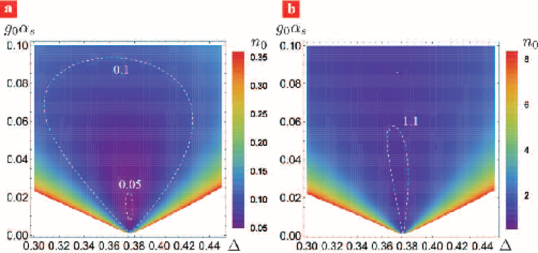
Figure 4: Cooling limit $n_{0}$ for oscillator 0. $\omega_{1}$ is set as the unit, with $\gamma_{0}=\gamma_{1}=10^{-6}$, $g_{1}\alpha_{s}=0.336$, $n_{0,th}=n_{1,th}=100$, and $\omega_{0}=0.7$. a) $\kappa=300$, such that $\kappa/\omega_{0}\approx 430$. In the region enclosed by the two white dashed circles, $\tilde{n}_{0}<0.1$ and 0.05, as indicated in the figure. b) $\kappa=7000$, such that $\kappa/\omega_{0}=10^{4}$, and $n_{0}<1.1$ in the region enclosed by the dashed line. In the uncolored regions, $n_{0}$ is too high to show.

IV Ground-state cooling: exact phonon-number solutions

In the previous section, we determined the possibility of ground-state cooling using quantum noise analysis. In this section, we shall examine this further by solving the linearized quantum Langevin equations exactly, i.e, Eqs. (12)–(14). Note that the expression for $\hat{b}_{0,\omega}$ is presented in the Appendix, as it is very complex. The exact result of the cooling limit $n_{0}$ is obtained from the integration

$$n_{0}=\int_{-\infty}^{\infty}\frac{d\omega}{2\pi}\frac{d\omega^{\prime}}{2\pi}\langle\hat{b}^{\dagger}_{0,\omega}\hat{b}_{0,\omega^{\prime}}\rangle.$$ (47)

IV.1 Cooling in the unresolved sideband regime

Firstly, we examine the prediction of ground-state cooling in the unresolved sideband regime. The dependence of $n_{0}$ on $g_{0}\alpha_{s}$ and $\Delta$ is illustrated in Fig. (4). This figure shows that the phonon number of the target oscillator $\tilde{n}_{0}$ can be reduced to less than $0.05$ when the sideband parameter $\kappa/\omega_{0}$ is approximately $430$. Moreover, when $\kappa/\omega_{0}$ is increased to $10^{4}$, $n_{0}\approx 1$ can still be decreased to approximately 1. (In comparison, the standard sideband cooling at $\Delta=-\kappa/2$ yields the optimal $n_{opt,0}=2500$.)

IV.2 Precision of quantum noise approach

The quantum noise approach is based on the Fermi golden rule, which is valid only for the weak limit. Fig. 4 also shows the region that is invisible to the quantum noise approach. This figure indicates that, when $g_{1}$ is fixed, optimal cooling is realized with proper $g_{0}$. However, the quantum noise approach naively suggests larger $g_{0}$.

To visualize the breakdown of the quantum noise approach, we note that $n_{0}$ is determined independently in terms of the laser-driving fluctuation noise, the local thermal environment noise, and the thermal environment of the ancillary oscillator. In Fig. 5, these contributions are illustrated separately. We find that the laser-driving fluctuation dominates the phonon source after $n_{0}$ has been obtained, as shown by the red line in Fig. 5. As the source of this contribution is independent of the thermal environment of the oscillators, it provides an intrinsic limit for the optically induced cooling.

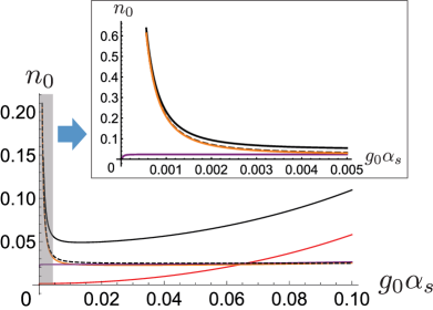
Figure 5: $n_{0}$ as function of $g_{0}$ (and magnified for weak couplings). $\omega_{1}$ is set as the unit, $\Delta=0.377$, and the other parameters are identical to those in Fig. 3. The black dashed line is the phonon occupation given by the quantum noise approach, the black solid line is the exact result for $n_{0}$, which is the sum of the three contributions from the laser driving fluctuation $\hat{d}_{in}$ (red), the local thermal environment $\hat{b}_{0,in}$ (orange), and the thermal environment of the ancillary oscillator $\hat{b}_{1,in}$ (purple).

The red line in Fig. 5, or the term for the photon number fluctuation noise, is ascribed to a term in the exact solution of $\hat{b}_{0,\omega}$ [Eq. (53) in the Appendix]:

$$\frac{-ig_{0}\alpha_{s}\sqrt{\kappa}\chi^{-1*}_{0,-\omega}}{\mathcal{N}[\omega]}\{\chi^{-1}_{c,\omega}\chi^{-1}_{1,\omega}\chi^{-1*}_{1,-\omega}$$ (48)

$$\qquad+i2\omega_{1}g_{1}^{2}\alpha_{s}^{2}(2\Delta^{2}-i\Delta\kappa-i\omega\kappa)\}\hat{d}^{\dagger}_{in,\omega}.$$

Here, $\mathcal{N}[\omega]$ is given as

$$\mathcal{N}[\omega]= \chi^{-1}_{c,\omega}\chi^{-1*}_{c,-\omega}\chi^{-1}_{0,\omega}\chi^{-1*}_{0,-\omega}N[\omega]$$ (49)

$$-4\omega_{0}\omega_{1}\kappa^{2}g_{0}^{2}g_{1}^{2}\alpha_{s}^{4}+4\Delta\omega_{0}g_{0}^{2}\alpha_{s}^{2}\chi^{-1}_{1,\omega}\chi^{-1*}_{1,-\omega}.$$

Further, $N[\omega]$ has already been given in Eq. (22). $1/\mathcal{N}[\omega]$ is actually the common factor of all the other terms involving $\hat{d}_{in}$, $\hat{b}_{0,in}$, and so on, and its poles determine the eigen-frequencies and damping rates of all the eigenmodes of the hybrid system.

The quantum noise approach functions well in the weak regime. In our derivation of $S_{nn}[\omega]$, we treat the optical mode and oscillator 1 as the steady background; this approach is valid if their dynamics are significantly faster than that of oscillator 0. Because we have $\kappa\gg\tilde{\gamma}_{1}\gg\gamma_{0}$, the quantum noise approach is effective, as verified by the magnified chart shown in Fig. 5.

It is emphasized that, in Fig. 5, there is a coincidence between the quantum noise predictions and the $n_{0}$ component contributed by the local environment, i.e., the orange lines obtained from the $\langle\hat{b}_{in,0,\omega}\hat{b}_{in,0,\omega^{\prime}}^{\dagger}\rangle$ and $\langle\hat{b}_{0,in,\omega}^{\dagger}\hat{b}_{0,in,\omega^{\prime}}\rangle$ terms in Eq. (47). This is reasonable, because only the $n_{0}$ contributions from the local noise decrease with increased $g_{0}$ (at least in the plotted region).

IV.3 Inverse relationship between $g_{1}\alpha_{s}$ and optimal detuning

In Sec. III.4.3, we have shown that the quantum noise approach suggests $\Delta\approx\omega_{0}/2$, along with an inverse relationship between $g_{1}\alpha_{s}$ and $\Delta$. Here, we examine the quantum noise approach using the exact solution of $n_{0}$ and illustrate the result in Fig. (6). The numerical result supports this statement very well. Additionally, it can be seen from Fig. (4) that the optimal detuning exhibits independence of the sideband parameter when $g_{0}\alpha_{s}$ is very close to zero. This feature also agrees with the theory presented in Sec. III.4.3.

Figure 6: Mean phonon number $n_{0}$ as a function of $g_{1}\alpha_{s}$ and the detuning $\Delta$. $\omega_{1}$ is set as the unit, with $\gamma_{0}=\gamma_{1}=10^{-6}$, $g_{0}\alpha_{s}=0.1$, $n_{0,th}=n_{1,th}=100$, and $\omega_{0}=0.7$. $\kappa=300$, such that $\kappa/\omega_{0}\approx 430$. In the region enclosed by the white dashed lines, $\tilde{n}_{0}<0.1$ and $0.05$, as indicated in the figure. The position of $\Delta=\omega_{0}/2$ is indicated by a short dashed line.

V Discussion

A remarkable proposal has demonstrated that strong and tunable dissipative coupling can be established by inserting a movable membrane in a Michelson-Sagnac interferometer diss-realize . Hence, a hybrid system of dispersively and dissipatively coupled oscillators can be constructed by replacing one fixed mirror within the interferometer with a movable one. Our scheme requires only a single optical mode with one driving mode. Therefore, in cases where more dissipatively coupled oscillators are accessible, our approach is significantly simpler than schemes involving ground-state cold atom ensembles or correlated multi-cavities. It is also simpler than those based on OMIT effects eit-2 ; eit-cooling , where two driving modes and an additional oscillator in the resolved sideband regime are required. From a practical perspective, the most important concern is successfully embedding a dissipative oscillator into other dispersive optomechanical systems to obtain ground-state cooling. We do not elaborate on this topic here, because only a small number of experimental demonstrations of dissipative optomechanical systems have been reported.

In the following, we discuss commonalities and conduct a comparison between the approach presented in this paper and the existing unresolved sideband cooling schemes. First, there are similarities between the Hamiltonians used in the various cooling schemes and that proposed here, characterized by $H_{int,1}$ [Eq. (6)]. In the OMIT scheme, the Hamiltonian (eit-cooling, , Eq. (49)) is

$$H_{int}=\hbar g_{2}(\hat{b}_{2}^{\dagger}+\hat{b}_{2})(\hat{a}^{\dagger}_{0}\hat{a}_{1}+\hat{a}^{\dagger}_{1}\hat{a}_{0}),$$ (50)

where $\hat{a}_{0/1}$ are the two required cavity modes. In the atom-optomechanical hybrid system, the Hamiltonian (atom-2015, , Eq. (3)) is

$$H_{int}=G_{0}(\hat{a}^{\dagger}\hat{c}+\hat{c}^{\dagger}\hat{a}),$$ (51)

where $\hat{a}$ and $\hat{c}$ correspond to the optical mode and collective operators of the atom ensemble, respectively. Finally, in the coupled-cavity scheme, the Hamiltonian (mt-cav-2015, , Eq. (A2)) is

$$H_{int}=J\hat{a}_{1}^{\dagger}\hat{a}_{2}+J^{*}\hat{a}_{2}^{\dagger}\hat{a}_{1},$$ (52)

where $\hat{a}_{1}$ is the optical mode coupled with the mechanical oscillator and $\hat{a}_{2}$ is the mode of the ancillary cavity, the line width of which must be significantly smaller than the resonant frequency of the target oscillator. It is quite interesting to note the similarities between these damping-like interactions. From this perspective, the ancillary oscillator serves as a medium in our scheme, and it is the input/environment mode that is essential for ground-state cooling. The ancillary oscillator plays a role similar to those of the ancillary cavities or ground-state atoms in the alternative schemes.

Next, we compare our scheme more closely with the OMIT scheme eit-cooling ; eit-2 , which is analogous to electromagnetically induced transparency. The OMIT scheme uses an ancillary oscillator that is dispersively coupled to the cavity mode. Its position spectrum is also embedded in the photon-number fluctuation spectrum. In addition, a significant imbalance between the two peaks of the position spectrum is necessary. Therefore, the ancillary dispersive oscillator must also be cooled to the ground state. However, as this oscillator is coupled dispersively, cooling is only possible if the resonant frequency is larger than the cavity line width. This leads to an extremely large gap between the frequencies of the two oscillators. In our notation, this large frequency gap means that the requirement $\omega_{0}\approx\tilde{\omega}_{1}$ cannot be satisfied. Thus, another largely detuned driving laser would be required in order to introduce the driving laser beat note, and unexpected and harmful excitation of some modes of the real mechanical system could be induced. (see (eit-cooling, , Sec. III.G.)). The method using the dissipative oscillator presented in this study avoids this problem.

VI Conclusion and Outlook

In this paper, we have proposed a new scheme for optomechanical cooling in the unresolved sideband regime, and we have verified this technique using both the quantum noise approach and exact solutions to the quantum Langevin equations. The proposed scheme uses a dispersively coupled oscillator that is also in the unresolved sideband regime. This ancillary oscillator significantly modifies the photon-number fluctuation spectrum and, thus, realizes ground-state cooling in the unresolved sideband regime. Therefore, the dissipatively coupled oscillator can cool not only itself, but also other mechanical oscillators coupled with the same optical mode. This scheme will enrich the optomechanical toolbox. Further, as dissipatively coupled systems have not been investigated widely, this result will stimulate further interest and related research questions.

As optomechanics facilitates the realization of controllable macroscopic quantum systems, it is feasible that this subject will play an increasingly important role in quantum metrology, quantum information processing, and, possibly, in future quantum computers. The very recent confirmation of gravitational waves using optomechanical technology gwave has strongly endorsed this confidence. The scheme developed in this article will enrich the optomechanical cooling toolbox. In addition, the use of dissipative coupling in cooling constitutes an example of beneficial exploitation of the noisy environment modes. Finally, as dissipatively coupled systems have not been investigated widely, we hope that this result will stimulate further interest in this topic, along with related research questions.

Appendix A Exact solution of phonon annihilation operator

The phonon annihilation operator $\hat{b}_{0,\omega}$ is expressed exactly as

$$\hat{b}_{0,\omega}= \frac{-ig_{0}\alpha_{s}\sqrt{\kappa}\chi^{-1*}_{0,-\omega}}{\mathcal{N}[\omega]}\{\chi^{-1*}_{c,-\omega}\chi^{-1}_{1,\omega}\chi^{-1*}_{1,-\omega}$$ (53)

$$\qquad+4i\omega_{1}g_{1}^{2}\alpha_{s}^{2}\Delta(i\kappa-\Delta)\}\hat{d}_{in,\omega}$$

$$+\frac{-ig_{0}\alpha_{s}\sqrt{\kappa}\chi^{-1*}_{0,-\omega}}{\mathcal{N}[\omega]}\{\chi^{-1}_{c,\omega}\chi^{-1}_{1,\omega}\chi^{-1*}_{1,-\omega}$$

$$\qquad+i2\omega_{1}g_{1}^{2}\alpha_{s}^{2}(2\Delta^{2}-i\Delta\kappa-i\omega\kappa)\}\hat{d}^{\dagger}_{in,\omega}$$

$$-\frac{\sqrt{\gamma_{0}}}{\mathcal{N}[\omega]}\{2ig_{0}^{2}\alpha_{s}^{2}(\kappa^{2}\omega_{1}g_{1}^{2}\alpha_{s}^{2}-\Delta\chi^{-1}_{1,\omega}\chi^{-1*}_{1,-\omega})$$

$$\qquad+\chi^{-1}_{c,\omega}\chi^{-1*}_{c,-\omega}\chi^{-1*}_{0,-\omega}N[\omega]\}\hat{b}_{in,0,\omega}$$

$$+\frac{2i\sqrt{\gamma_{0}}g_{0}^{2}\alpha_{s}^{2}}{\mathcal{N}[\omega]}(\Delta\chi^{-1}_{1,\omega}\chi^{-1*}_{1,-\omega}-\omega_{1}\kappa^{2}g_{1}^{2}\alpha_{s}^{2})\hat{b}_{in,0,\omega}^{\dagger}$$

$$+\frac{g_{0}^{2}g_{1}^{2}\alpha_{s}^{4}\chi^{-1*}_{0,-\omega}\sqrt{\gamma_{1}}}{2\mathcal{N}[\omega]}(i\kappa^{2}+2\kappa\omega-4i\Delta^{2})$$

$$\qquad\times(\chi^{-1*}_{1,-\omega}\hat{b}_{in,1,\omega}+\chi_{1,\omega}^{-1}\hat{b}^{\dagger}_{in,1,\omega}).$$

References

- (1) M. D. LaHaye, O. Buu, B. Camarota, and K. C. Schwab, Science 304, 74 (2004).
- (2) J. D. Teufel, T. Donner, M. A. Castellanos-Beltran, J. W. Harlow, and K. W. Lehnert, Nat. Nanotechnol. 4, 820 (2009).
- (3) A. G. Krause, M. Winger, T. D. Blasius, Q. Lin, and O. Painter, Nat. Photon. 6, 768 (2012).
- (4) Y.-W. Hu, Y.-F. Xiao, Y.-C. Liu, and Q. Gong, Front. Phys. 8, 475 (2013).
- (5) L. F. Buchmann, H. Jing, C. Raman, and P. Meystre, Phys. Rev. A 87, 031601(R) (2013).
- (6) T. P. Purdy, R. W. Peterson, and C. A. Regal, Science 339, 801 (2013).
- (7) V. Fiore, Y. Yang, M. C. Kuzyk, R. Barbour, L. Tian, and H. Wang, Phys. Rev. Lett. 107, 133601 (2011).
- (8) Y.-D. Wang and A. A. Clerk, Phys. Rev. Lett. 108, 153603 (2012).
- (9) C. Dong, V. Fiore, M. C. Kuzyk, and H. Wang, Science 338, 1609 (2012).
- (10) M. Schmidt, M. Ludwig, and F. Marquardt, New. J. Phys. 14, 125005 (2012).
- (11) K. Stannigel, P. Komar, S. J. M. Habraken, S. D. Bennett, M. D. Lukin, P. Zoller, and P. Rabl, Phys. Rev. Lett. 109, 013603 (2012).
- (12) O. Romero-Isart, A. C. Pflanzer, F. Blaser, R. Kaltenbaek, N. Kiesel, M. Aspelmeyer, and J. I. Cirac, Phys. Rev. Lett. 107, 020405 (2011).
- (13) B. Pepper, R. Ghobadi, E. Jeffrey, C. Simon, and D. Bouwmeester, Phys. Rev. Lett. 109, 023601 (2012).
- (14) P. Sekatski, M. Aspelmeyer, and N. Sangouard, Phys. Rev. Lett. 112, 080502 (2014).
- (15) T. Rocheleau, T. Ndukum, C. Macklin, J. B. Hertzberg, A. A. Clerk, and K. C. Schwab, Nature (London) 463, 72 (2010).
- (16) J. D. Teufel, T. Donner, D. Li, J. W. Harlow, M. S. Allman, K. Cicak, A. J. Sirois, J. D. Whittaker, and R. W. Simmonds, Nature (London) 475, 359 (2011)
- (17) E. Verhagen, S. Deléglise, S. Weis, A. Schliesser, and T. J. Kippenberg, Nature (London) 482, 63 (2012).
- (18) J. Chan, T. P. M. Alegre, A. H. Safavi-Naeini, J. T. Hill, A. Krause, S. Gröblacher, M. Aspelmeyer, and O. Painter, Nature (London) 478, 89 (2011).
- (19) S. Mancini, D. Vitali, and P. Tombesi, Phys. Rev. Lett. 80, 688 (1998).
- (20) P.-F. Cohadon, A. Heidmann, and M. Pinard, Phys. Rev. Lett. 83, 3174 (1999).
- (21) D. Kleckner and D. Bouwmeester, Nature (London) 444, 75 (2006).
- (22) T. Corbitt, C. Wipf, T. Bodiya, D. Ottaway, D. Sigg, N. Smith, S. Whitcomb, and N. Mavalvala, Phys. Rev. Lett. 99, 160801 (2007).
- (23) M. Poggio, C. L. Degen, H. J. Mamin, and D. Rugar, Phys. Rev. Lett. 99, 017201 (2007).
- (24) T. J. Kippenberg and K. J. Vahala, Science 321, 1172 (2008).
- (25) F. Marquardt and S. M. Girvin, Physics 2, 40 (2009).
- (26) M. Aspelmeyer, T. J. Kippenberg, and F. Marquardt, Rev. Mod. Phys. 86, 1391 (2014).
- (27) Y. Chen, J. Phys. B: At. Mol. Opt. Phys. 46 104001 (2013).
- (28) Y.-C. Liu, Y.-W. Hu, C. W. Wong, and Y.-F. Xiao, Chin. Phys. B 22, 114213 (2013).
- (29) M. Eichenfield, J. Chan, R. M. Camacho, K. J. Vahala, and O. Painter, Nature (London) 462, 78 (2009).
- (30) C. Genes, D. Vitali, P. Tombesi, S. Gigan, and M. Aspelmeyer, Phys. Rev. A 77, 033804 (2008).
- (31) F. Marquardt, J. P. Chen, A. A. Clerk, and S. M. Girvin, Phys. Rev. Lett. 99, 093902 (2007).
- (32) I. Wilson-Rae, N. Nooshi, W. Zwerger, and T. J. Kippenberg, Phys. Rev. Lett. 99, 093901 (2007).
- (33) T. Ojanen and K. Børkje, Phys. Rev. A 90, 013824 (2014).
- (34) Y.-C. Liu, Y.-F. Xiao, X. S. Luan, and C. W. Wong, Sci. China Phys. Mech. Astron. 58, 050305 (2015).
- (35) Y. Guo, K. Li, W. Nie, and Y. Li, Phys. Rev. A 90, 053841 (2014).
- (36) Y.-C. Liu, Y.-F. Xiao, X. Luan, Q. Gong, and C. W. Wong, Phys. Rev. A 91, 033818 (2015).
- (37) C. Genes, H. Ritsch, and D. Vitali, Phys. Rev. A 80, 061803(R) (2009).
- (38) K. Hammerer, K. Stannigel, C. Genes, P. Zoller, P. Treutlein, S. Camerer, D. Hunger, and T. W. Hänsch, Phys. Rev. A 82, 021803(R) (2010).
- (39) C. Genes, H. Ritsch, M. Drewsen, and A. Dantan, Phys. Rev. A 84, 051801(R) (2011).
- (40) S. Camerer, M. Korppi, A. Jöckel, D. Hunger, T. W. Hänsch, and P. Treutlein, Phys. Rev. Lett. 107, 223001 (2011).
- (41) B. Vogell, K. Stannigel, P. Zoller, K. Hammerer, M. T. Rakher, M. Korppi, A. Jöckel, and P. Treutlein, Phys. Rev. A 87, 023816 (2013).
- (42) T. P. Purdy, D. W. C. Brooks, T. Botter, N. Brahms, Z.-Y. Ma, and D. M. Stamper-Kurn, Phys. Rev. Lett. 105 133602 (2010).
- (43) F. Bariani, S. Singh, L. F. Buchmann, M. Vengalattore, and P. Meystre, Phys. Rev. A 90, 033838 (2014).
- (44) X. Chen, Y.-C. Liu, P. Peng, Y. Zhi, and Y.-F. Xiao, Phys. Rev. A 92, 033841 (2015).
- (45) J. S. Bennett, K. Khosla, L. S. Madsen, H. Rubinsztein-Dunlop, and W. P. Bowen, arXiv:1510.05368 (2015).
- (46) J. Aasi et al. (The LIGO Scientific Collaboration), Class. and Quantum Grav. 32, 074001 (2015).
- (47) F. Elste, S. M. Girvin, and A. A. Clerk, Phys. Rev. Lett. 102, 207209 (2009).
- (48) M. Li, W. H. P. Pernice, and H. X. Tang, Phys. Rev. Lett. 103, 223901 (2009).
- (49) M. Wu, A. C. Hryciw, C. Healey, D. P. Lake, H. Jayakumar, M. R. Freeman, J. P. Davis, and P. E. Barclay, Phys. Rev. X 4, 021052 (2014).
- (50) A. Xuereb, R. Schnabel, and K. Hammerer, Phys. Rev. Lett. 107, 213604 (2011).
- (51) A. Sawadsky, H. Kaufer, R. M. Nia, S. P. Tarabrin, F. Ya. Khalili, K. Hammerer, and R. Schnabel, Phys. Rev. Lett. 114, 043601 (2015).
- (52) T. Weiss, C. Bruder, and A. Nunnenkamp, New J. Phys. 15, 045017 (2013).
- (53) T. Weiss and A. Nunnenkamp, Phys. Rev. A 88, 023850 (2013).
- (54) S. P. Tarabrin, H. Kaufer, F. Ya. Khalili, R. Schnabel, and K. Hammerer, Phys. Rev. A 88, 023809, (2013).
- (55) N. Vostrosablin and S. P. Vyatchanin, Phys. Rev. D 89, 062005 (2014).
- (56) A. A. Clerk, M. H. Devoret, S. M. Girvin, F. Marquardt, and R. J. Schoelkopf, Rev. Mod. Phys. 82, 1155 (2010).
- (57) B. P. Abbott et al. (LIGO Scientific Collaboration and Virgo Collaboration), Phys. Rev. Lett. 116, 061102 (2016).