Using Symmetry to Schedule Classical Matrix Multiplication

Abstract

Presented with a new machine with a specific interconnect topology, algorithm designers use intuition about the symmetry of the algorithm to design time and communication-efficient schedules that map the algorithm to the machine. Is there a systematic procedure for designing schedules? We present a new technique to design schedules for algorithms with no non-trivial dependencies, focusing on the classical matrix multiplication algorithm.

We model the symmetry of algorithm with the set of instructions $X$ as the action of the group $\mathfrak{S}_{X}$ formed by the compositions of bijections from the set $X$ to itself. We model the machine as the action of the group $N\times\Delta$, where $N$ and $\Delta$ represent the interconnect topology and time increments respectively, on the set $P\times T$ of processors iterated over “time steps”. We model schedules as “symmetry-preserving” equivariant maps between the set $X$ and a subgroup of its symmetry $\mathfrak{S}_{X}$ and the set $P\times T$ with the symmetry $N\times\mathbb{Z}$. Such equivariant maps are the solutions of a set of algebraic equations involving group homomorphisms. We associate time and communication costs with the solutions to these equations.

We solve these equations for the classical matrix multiplication algorithm and show that equivariant maps correspond to time- and communication-efficient schedules for many topologies. We recover well known variants including the Cannon’s algorithm [7] and the communication-avoiding “2.5D” algorithm [38] for toroidal interconnects, systolic computation for planar hexagonal VLSI arrays [24], recursive algorithms for fat-trees [29], the cache-oblivious algorithm for the ideal cache model [16], and the space-bounded schedule [10, 5] for the parallel memory hierarchy model [2]. This suggests that the design of a schedule for a new class of machines can be motivated by solutions to algebraic equations.

1 Introduction

Parallel computers are varied in their network and memory characteristics so that no single version of an algorithm for a problem works uniformly well across all machines. This poses a recurring challenge to algorithm designers who are forced to engineer “new algorithms” for a target machine. Research literature as well as textbooks on parallel algorithms [28] list dozens of variants for such algorithms that are suited to different network topologies and memory hierarchies. Algorithms for fundamental problems like matrix multiplication are re-engineered for every new architecture.

Many of these “new algorithms” are often simply a new schedule or a different data layout of a well known algorithm. The redesign optimizes the location and the order of execution of the instructions in the algorithm to minimize communication and running time on the target machine. This machine-specific schedule design is, more often that not, done through human intuition about the symmetry of the algorithm and the machine, as opposed to a systematic or automated procedure. We address this gap in the case of algorithms with no non-trivial dependencies – algorithms whose instructions can be executed in any order (e.g. matrix multiplication, direct n-body methods, tensor contractions). We propose models for capturing the symmetry of such algorithms and machine characteristics (network topology and memory hierarchy), and show how to use these models systematically.

Our approach is inspired by three simple observations. First, the transformations which leave a set invariant form a group, called the symmetry group of the set. The transformations can be seen as the “actions” of this group on the set. Therefore, we model the symmetry of an algorithm as the group $\mathfrak{S}_{X}$ of the symmetries of its instruction set $X$.

Second, many machines can be described as the action of a group that models the interconnect ($N$) on the set of nodes some of which have processing elements ($P$). Similarly time can be modeled as the action of a group representing time increments ($\Delta$) on the set representing time steps ($T$). Putting these two together, the movement of data over the network between time steps can be modelled as the action of the group $N\times\Delta$ on the set $P\times T$.

Third, the schedules of common variants of algorithms seem to be “symmetry-preserving” maps from the instruction set $X$ to the set $P\times T$ that preserve some subset of the symmetries of $X$. Such schedules can be modelled as “equivariant” maps from $X$ to $P\times T$ that commute with the group actions on these sets. That is, the equivariant map and an action of the symmetry group can be applied to an element $x\in X$ in any order with the same result (Fig. 3).

Therefore, we pose the problem of finding a machine-specific schedule and data layout for an algorithm as one of finding equivariant maps, thus narrowing our search significantly. We also associate time and communication costs with these solutions (Section 2). The problem is then reduced to finding the optimal solution to an instance of algebraic equations. The solutions to these equations correspond to homomorphisms between subgroups of the symmetry group $\mathfrak{S}_{X}$ and the group $N\times\Delta$ (Section 3). We use knowledge of the structure of these groups to enumerate and optimize over feasible solutions.

We demonstrate the effectiveness of this technique with the example of the classical matrix multiplication algorithm. The instructions of this algorithm are indexed by three arrays. Assuming that the addition is commutative, the indices in each array may be permuted in any order. Therefore, the symmetry group of the matrix multiplication algorithm can be expressed as a product of three permutation groups (group consisting of permutation of an array) corresponding to the three indices. The subgroups of a permutation group (a.k.a. symmetric group) are well-understood [31]. We use this knowledge to derive cost-efficient schedules for various machines, recovering several well-known variants of classical matrix multiplication (Section 4).

Although individual technical results in this paper are not radically new, the principal contribution of the paper is a fresh and unifying perspective to the problem of schedule design. The tools and the line of reasoning developed in this paper can be used to systematically derive schedules for future architectures or reason about different data layouts.

Related Work. One approach to systematically adapt algorithms to machines consists of the oblivious paradigms [4, 10, 5] which propose automatic—even online—schedules for machines with tree-like interconnects. The machines these models represent can be shown to be capable of executing efficient variants of any parallel algorithm competitively compared to any other architecture with the same hardware resource constraints (such as VLSI area). Algorithms that are provably (asymptotically) optimal for such machines when coupled with these schedules can be designed [9, 6, 37, 4] and achieve competitive performance. However, this approach can not generate the best schedule for any topology.

Another tool for developing schedules is the Polyhedral Model (also called the Polytope model) [30, 15]. This model has its roots in the analysis of recurrence equations [21] and automatic parallelization of “DO-loops” [25]. The principal aim of the model was parallelization of nested loops for vector architectures. The problem was modeled as Parallel Integer Programming [13] giving rise to many code-generation tools [3, 35]. Loop transformation techniques based on affine transformations for improving the performance of nested loops were proposed [40, 32], and blocking for locality was considered [39]. A number of features were incrementally added to the Polyhedron model including the notion of multi-dimensional time [14], data replication for reducing communication and synchronization [8], and memory management [34, 12, 27]. Some of these results are summarized in [18]. Similar efforts for adapting algorithms to systolic arrays include [33, 23, 36].

Our work differs from previous work in that it is based on groups and their homomorphisms rather than affine transformations which are the basis for most previous work. Since groups are more expressive, our model elegantly captures many of the features that were incrementally retrofitted to earlier models such as data layout, data movement, schedules, multiple copies of data and multi-dimensional time. The model is succinct enough to be represented in a diagram (Fig. 1) which we will proceed to explain.

Figure 1: A commutative diagram summarizing all the symmetry-preserving maps described in Section 2. The set $X$ represents the instructions in the algorithm, the set $(\cup_{i=1}^{c}I^{(i)})\times T$ represents $c$ copies of the input set $I$ iterated over time, and $(P\cup M)\times T$ represents the set of processors and memory units iterated over time. The group action over each of these sets is depicted with a text-overlaid arrow. The equivariant maps between these sets are shown in red and are to be solved for. These are the functions $f$, which determines the schedule, $l_{I}$, which determines the data placement, and $d_{I}$, which determines the time and the copy of variable in each variable set used for an instruction. Similar equations can be written for other input and output sets.

2 Models for Computation, Machine and Symmetry-Preserving Maps

We present models for the symmetries of an algorithm in which instructions can be executed in any order (Sec. 2.1), and the topology of the target machine (Sec. 2.2). Schedules are defined as maps from the instruction set to the set of processors iterated over time. We will formalize the notion of symmetry-preserving maps and represent it as commutative diagrams. We also incorporate data placements and data movements in to these models (Sec. 2.3). We assign costs to the maps corresponding to schedules and data movement (Sec. 2.4) and add more features to the model (Sec. 2.5).

2.1 Computation model and symmetries

An algorithm consists of a finite set of instructions $X$ and a finite set of input and output variable sets. Each instruction accesses one variable from each input and output variable set so that $X$ is a subset of the direct product of the variable sets. For classical matrix multiplication the input variable sets are the variables denoting the entries of the two input matrices, and the output variable set corresponds to output matrix. Let $[n]$ denote the set $\{0,1,\dots,n-1\}$. For a size $l\times m\times n$ multiplication, the input variable sets are $A=\{A_{rr^{\prime}}\}_{r\in[l],r^{\prime}\in[m]}$ and $B=\{B_{rr^{\prime}}\}_{r\in[m],r^{\prime}\in[n]}$, and the output variable set is $C=\{C_{rr^{\prime}}\}_{r\in[n],r^{\prime}\in[l]}$. The set of instructions $X$ is $\{(A_{ij},B_{jk},C_{ki})\}_{i\in[l],j\in[m],k\in[n]}\subset A\times B\times C$.

Groups are a standard way to model the symmetries of a set (see Appendix A for definitions of groups, homomorphisms and group actions). Consider all bijections (invertible functions) from the set $X$ to itself. These operations form a group under composition. This is referred to as the symmetry group $\mathfrak{S}_{X}$ of $X$. The symmetry group $\mathfrak{S}_{X}$ acts naturally on the set $X$: the action $\sigma\cdot$ of each element $\sigma\in\mathfrak{S}_{X}$ is the bijective map that $\sigma$ represents. We denote this group action diagrammatically by

The group action can also be seen as the graph with vertex set $X$ and edges $x\mapsto\sigma\cdot x$ for each $x\in X$ and $\sigma\in\mathfrak{S}_{X}$.

In the case of matrix multiplication, the bijections correspond to separate permutations on the indices $i\in[l]$, $j\in[m]$ and $k\in[n]$ (we assume += in $C_{ki}$+=$A_{ij}\cdot B_{jk}$ is associative and commutative). The group formed by the permutations of $n$ numbers (or symbols) under the composition operation is called the symmetric group of $n$ numbers, and denoted by $S_{n}$. Therefore, the symmetry group of the set of instructions of classical matrix multiplication algorithm is isomorphic to the direct product of three symmetric groups $S_{l}$, $S_{m}$ and $S_{n}$: $\mathfrak{S}_{X}\cong S_{l}\times S_{m}\times S_{n}$. So we have

where $S_{l}$, $S_{m}$ and $S_{n}$ act on indices $i,j$ and $k$ respectively. In this case, the graph corresponding to the group action has vertices $X_{ijk}$ indexed by $i,j$ and $k$. If a triplet of permutations on $[l],[m]$ and $[n]$ take the indices $i$ to $i^{\prime}$, $j$ to $j^{\prime}$ and $k$ to $k^{\prime}$ respectively, then there is an edge between vertices $X_{ijk}$ and $X_{i^{\prime}j^{\prime}k^{\prime}}$ labelled with this triplet of permutations.

We can similarly model the symmetry of an input set $I$:

For matrix multiplication, we have for the input set $A$,

where $S_{l}$ and $S_{m}$ act on the indices $r$ and $r^{\prime}$ respectively.

2.2 Models for machine topology

A machine consists of a set of nodes connected by a network. Each node consists of a finite amount of memory. Some nodes also have a sequential processing element and we refer to such a node as a processor. For simplicity, we will deal with the case where all nodes are processors until Sec. 2.5. Just as in the computation model, we will model the machine as a group action on a set.

We start with the simple example of a “2D-torus” machine consisting of $q\times q$ processors connected with a 2D-torus network. The network can be modeled as the group $\left(\mathbb{Z}/{q}\mathbb{Z}\right)^{2}$ where $(\mathbb{Z}/q\mathbb{Z})$ is the group of integers $\{0,1,\dots,q-1\}$ with the group operation ’$+_{q}$’, addition modulo $q$. The group element $(i,j)$ indicates traversing $i$ hops to the right and $j$ hops upwards (with wrap-around), and $(-i,-j)$ represents $i$ hops to the left and $j$ hops downwards. The machine can be modeled as the action of the network group $N:=\left(\mathbb{Z}/{q}\mathbb{Z}\right)^{2}$ on the processor set $P=\{P_{xy}\}_{x\in[q],y\in[q]}$. The element $(i,j)\in N$ maps $(i,j)\cdot P_{x,y}\mapsto P_{i+_{q}x,j+_{q}y}$ indicating the relative position of these two processors.

We add the notion of time steps (not necessarily clock cycles) to the model with the set $T$. A machine with synchronous time steps across the processors is modeled as the set $P\times T$ representing the processor set iterated over time steps. Time increments are modeled as the action of the time increment group $\Delta$ on the set $T$. For example, when a machine works for $t$ time steps all of the same duration, $T$ is represented by the set $\{t_{i}\}_{i\in[t]}$, and the increment by the action of $\Delta=\mathbb{Z}/{t}\mathbb{Z}$ over $T$. The set of possible data movements (communication) over the machine is modeled as the action of the group $N\times\Delta$ on the set $P\times T$. We represent it diagrammatically by

For a 2D-torus with synchronous and uniform time steps, $((i,j),t^{\prime})\cdot(P_{x,y},t_{0})\mapsto(P_{x+_{q}i,y+_{q}j},t_{0}+_{t}t^{\prime})$ corresponds to moving all the variables at the processor $P_{x,y}$ at time step $t$ to the processor $P_{x+_{q}i,y+_{q}j}$ at step $t^{\prime}$ (Fig. 2 left).

Figure 2: (left) Communication model of a 2D-torus of size $3\times 3$; group action in blue. (right) Fat-tree interconnect with 16 processors (black circles).

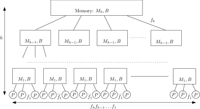
Figure 14: A Parallel Memory Hierarchy [2]. $M_{i}$ represent the sizes of the cache, $B$ represent cache line size. We set $B=1$ (this can be relaxed). $f_{i}$ represents the fan-out at each level. Number of processors, which are at the leaves, is $f_{h}f_{h-1}\dots f_{1}$.

Often, it is natural to consider time steps that are not of the same duration. For instance, for tree-like machines such as in the case of machine with fat-tree network [29] (Fig. 2 right; see Sec. 2.5 for a model for fat-tree) or parallel memory hierarchies [2] (Fig. 14), it is natural to consider schedules that progress in time steps of different granularity, one corresponding to each level in the tree. For this, we can model time steps as the set $T=T_{1}\times T_{2}\times\dots T_{k}$, where each $T_{l+1}:=\{t_{l,i}\}_{i\in[t_{l}]}$ represents $t_{l}$ steps within a $T_{l}$ superstep. The group $\Delta=\prod_{l\in[k]}\mathbb{Z}/{t_{l}}\mathbb{Z}$ acting on $T$ models time increments at each granularity.

2.3 Equations for schedule and data placement

A schedule is a map from the set of instructions $X$ to the set of processors iterated over time $P\times T$. We consider those schedules that are symmetry-preserving equivariant maps.

Definition 1 (Equivariant maps).

Fix the action of the group $G$ on the set $X$, and the action of the group $H$ on the set $Y$. A map $f:X\rightarrow Y$ is $(G,H)_{\rho}$-equivariant for the group homomorphism $\rho:G\rightarrow H$ if $f(g\cdot x)=\rho(g)\cdot f(x)$ for all elements $x\in X$ and the actions of $g\in G$ and $\rho(g)\in H$. A $(G,G)_{Id}$-equivariant map is simply called $G$-equivariant.

Figure 3: Commutative diagram depicting the $(G,H)_{\rho}$-equivariant map $f$ for the homomorphism $\rho:G\rightarrow H$. The diagram on the left indicates that the function $f:X\rightarrow Y$ makes the diagram on the right commute (different paths lead to the same answer) for all choices of elements $x\in X,y\in Y$ s.t. $y=f(x)$ and the actions of elements $g\in G,h\in H$ s.t. $h=\rho(g)$.

The commutative diagram above can also be seen as a graph homomorphism. Let $A$ and $B$ be the graphs corresponding to the action of the group $G$ on $X$ and group $H$ on $Y$. The edge map defined by the group homomorphism (blue arrow) and the vertex map defined by the equivarant map (red arrow) define a graph homomorphism from $A$ to $B$. The rest of the paper uses algebra to parameterize such graph homomorphisms and reason about their costs.

The schedule $f$ is modeled as an $(G,N\times\Delta)_{\rho}$-equivariant map from $X$ to $P\times T$ for some choice of subgroup $G\leq\mathfrak{S}_{X}$ of the symmetries of $X$ and homomorphism $\rho:G\rightarrow N\times\Delta$ (Fig. 4). The choice of subgroup $G$ and the homomorphism to $N\times\Delta$ significantly narrows down the possible equivariant maps to a few parameters (Sec. 3).

To trace the movement of the input variables over time, we consider the set $I\times T$, and define the action of the group $\mathfrak{S}_{I}\times\Delta$ on the set $I\times T$ as the natural extension of the action of $\mathfrak{S}_{I}$ on $I$ and the action of $\Delta$ on $t\in T$ (similar to the case of $P\times T$). We denote this by

The location of the input set $I$ on the machine is modeled as an $(H\times\Delta,N\times\Delta)_{\rho_{d}}$-equivariant map from the set $I\times T$ to the set $P\times T$, for some subgroup $H\leq\mathfrak{S}_{I}$ and homomorphism $\rho_{d}:H\times\Delta\rightarrow N\times\Delta$ of the form

$$\rho_{d}=(\mu:H\times\Delta\rightarrow N)\times Id_{\Delta},$$

where $\mu$ reflects its movement across time steps. Similar equations can be written for other input and output sets.

Figure 4: Commutative diagrams depicting the schedule $f$ and data placement function $l_{I}$ in red.

The schedule and data placement have to be consistent with each other so that the input or output element required by an instruction at a particular processor and time is present there. We model this constraint as an $(G,H\times\Delta)_{\rho_{l}}$-equivariant map $d_{I}:X\rightarrow I\times T$. For consistency, we add the constraint $\rho=\rho_{d}\circ\rho_{l}$.

Figure 5: The equivariant maps for the input set $I$ are shown in red and are to be solved for.

The commutative diagram in Fig. 5 represents a set of constraints that a valid schedule and data placement must satisfy. The principal constraint here that narrows the search for a schedule is equivariance. Further constraints include memory limits at each node. To find a feasible schedule and data placement, we “solve” this diagram for different choices of homomorphisms (see Sec. 3 for details). Each solution can be assigned time and communication costs as in Sec. 2.4.

2.4 Time and Communication Costs

A span of $t$ clock cycles, represented by the set $T_{C}$, is modeled as the action of $\mathbb{Z}/{t}\mathbb{Z}$ on $T_{C}$. The instructions in a schedule can be assigned time by projecting $P\times T$ down to $T$ and further down to clock cycles $T_{C}$ (the function $\pi_{T}$ in Fig. 6). The homomorphism $\rho_{T}:N\times\Delta\rightarrow\mathbb{Z}/{t}\mathbb{Z}$ flattens and scales time steps. We consider only those $\rho_{T}$ that disregard $N$, $\rho_{T}:n\times e_{\Delta}\mapsto e_{\mathbb{Z}/{t}\mathbb{Z}}$ for all $n\in N$, so that we can overload the notation $\rho_{T}$ with $\rho_{T}:\Delta\rightarrow\mathbb{Z}/{t}\mathbb{Z}$. If we have $\Delta=\mathbb{Z}/{t}\mathbb{Z}$ and each time step is five processor cycles long, we have $\rho_{T}:x\mapsto 5x$. We can flatten $k$ nested levels of supersteps with $2$ steps per level, that is $T=\prod_{l\in[k]}\{t_{l,0},t_{l,1}\}$ and $\Delta=(\mathbb{Z}/{2}\mathbb{Z})^{k}$, using $\rho_{T}:(\mathbb{Z}/{2}\mathbb{Z})^{k}\rightarrow\mathbb{Z}/{2^{k}}\mathbb{Z}$ that maps $\rho_{T}:(0,.._{i-1},1,0,..)\mapsto 2^{i-1}$ so that the $l$-th level superstep lasts for $2^{l}$ clock cycles. We can choose any combination of stretching and flattening to model the number of clock cycles needed for communication between supersteps.

Figure 6: Time can be traced with the function $f\circ\pi_{T}$ and communication cost with the homomorphism $\nu$.

The function $l_{I}$ describes the location of the variables in the input set $I$ at different time steps. The communication cost associated with a schedule is the cost of moving $I$ (and other input and output variable sets) to the processor specified by $l_{I}$ between time steps. When multiple paths are available, the cost is calculated for a specified routing policy.

Since $l_{I}$ is equivariant with $\rho_{d}$ which is of the form $\mu\times Id_{\Delta}$, the homomorphism $\mu:H\times\Delta\rightarrow N$ can be used to trace the movement of $I$ between time steps. The homomorphism $\mu$ restricted to $e_{\Delta}$ reflects the layout of the variable set at some time step. Further, $\mu$ can be seen as a function parameterized by time increments $\Delta$ that defines the network group element that moves variables in the set $I$ through the machine. Therefore assigning communication costs to elements of $N$ (according to some routing policy) defines the cost of a schedule. We simply add up the costs of network elements used across time steps (this equivalence is established by the equivariance property). When $\mu$ depends only on $\Delta$, each element is moved between time steps by the same $n\in N$ making it easy to calculate the communication cost.

2.5 Further details of the model

A schedule $f$ requires a certain number of variables to be present on a node at each time step. Those schedules that exceed the memory budget are not considered. On the other hand, when the memory available across the machines is larger than required for one copy of the variable sets, replicating variables across nodes is often necessary to design schedules that minimize communication [20]. Therefore we extend the model to allow a constant number of copies of each variable in an input set. The symmetry of $c$ copies of input set iterated across time steps is

Suppose a machine has nodes without a processor (call these $M$), we model the machine as the action of $N\times\Delta$ on $(P\cup M)\times T$. As before, the schedule $f$ is a $(G,N\times\Delta)_{\rho}$-equivariant map for some $G\leq\mathfrak{S}_{X}$. The important difference is that the image of $\rho$ must be a subset of $P\times T$.

All of the symmetries, group actions and equivariant maps are summarized in the commutative diagram in Fig. 1. We omit the homomorphisms and depict the action of the entire group in the text-overlaid arrow instead of just the subgroups relevant to the chosen homomorphism.

We conclude this section with a model for the fat-tree network (Fig. 2 right). A fat-tree of size $n=2^{k}$ is a $k$-level balanced binary tree with $n$ processors at the leaves. To send a message from processor $P_{i}$ to $P_{j}$, the fat-tree routes it up from $P_{i}$ to the least common ancestor of $P_{i}$ and $P_{j}$ in the tree and back down to $P_{j}$. We model this multi-level data movement as the action of a group that is the wreath product of the groups corresponding to per-level movement.

Definition 2 (wreath product).

The wreath product of two finite groups $A$ and $B$ for a specified action of the group $B$ on the finite set $\Omega$ is denoted by $A\wr_{\Omega}B$ and defined as the group action of $B$ on $|\Omega|$-tuples of the elements of $A$: $A\wr_{\Omega}B:=K\rtimes B$, where $K=\prod_{\omega\in\Omega}A_{\omega}$ and $\rtimes$ represents the action. When the index set $\Omega$ and the action of $B$ on $\Omega$ are clear from the context, such as in the case of $\Omega=[b]$ and $B=S_{b}$, we simply write $A\wr B$.

The elements of the group $S_{a}\wr S_{b}=(S_{a})^{b}\rtimes S_{b}\leq S_{ab}$ correspond to those permutations on the set $[ab]$ that result from some permutation within each of the partitions of the $ab$ elements into $\{0,..,a-1\},\{a,..,2a-1\},..,\{(b-1)a,..,ab-1\}$, followed by some permutation over the partitions.

We model a fat-tree network of size $n=2^{k}$ with the group action of the $k$-fold iterated wreath product

$$S_{2}^{\wr{k}}:=(((S_{2}\wr S_{2})\wr S_{2})\wr\dots S_{2}.$$

The action of the elements of $S_{2}^{\wr{k}}$ can be understood by organizing the $n=2^{k}$ elements into a $k$-level balanced binary tree. At each internal node in the binary tree, we can choose to either swap the left and right subtree or leave them as is. Each set of choices corresponds to a unique element in $S_{2}^{\wr{k}}$. When considered as the network group, the element $\sigma\in S_{2}^{\wr{k}}$ that sends index $i$ to the index $j$ ($i,j\in[n]$) sends the processor $P_{i}$ to $P_{j}$: $\sigma\cdot P_{i}\mapsto P_{j}$. Note that multiple permutations send $P_{i}$ to $P_{j}$ for any choice of $i,j\in[n]$. They number $2^{n-1}/n$ out of the total $2^{n-1}$ elements in this group.

3 Solving Commutative Diagrams for Equivariant Maps

The diagram in Fig. 1 is a set of constraints that the equivariant maps (in red) must satisfy for some choice of homomorphisms between subgroups of the groups whose actions are depicted. To find good schedules, we

• identify subgroups of the symmetry group $\mathfrak{S}_{X}$ of $X$,

• enumerate homomorphisms from this subgroup to other groups ($N,\Delta,\mathfrak{S}_{I}$, etc.),

• “solve the commutative diagram” for equivariant maps with respect to the homomorphism, and

• find the map with the least time and communication cost, eliminating those that violate memory constraints.

By “solving a commutative diagram” such as Fig. 3 for $(G,H)_{\rho}$-invariant maps for a homomorphism $\rho:G\rightarrow H$ and a fixed action of group $G$ on $X$ and $H$ on $Y$, we mean enumerating the maps $f:X\rightarrow Y$ that satisfy $f(g\cdot x)=\rho(g)\cdot f(x)$ for all $x\in X,g\in G$. Solving a multi-level commutative diagram such as in Fig. 1 or 5 entails finding functions that make each individual square in the diagram commute.

We will start with the solutions to the special case $H:=G$ and $\rho:=Id$ as in Fig. 7, which we simply refer to as $G$-equivariant maps. The general case will be similar.

Figure 7: Commutative diagram depicting the $G$-equivariant map $f:X\rightarrow Y$. Given an action $g\cdot$ of elements $g\in G$, the function $f$ makes the diagram commute for all $g\in G$ and $x\in X,y\in Y$ s.t. $y=f(x)$.

For a subgroup $K\leq G$, the quotient $G/K$ is a set of cosets of the form $aK$ for some $a\in G$, where $aK$ is the set $\{ak\ |\ k\in K\}$. All cosets of $K$ are of the same cardinality, and there are $|G|/|K|$ distinct cosets. We will see that $G$-equivariant maps from the set $X$ to $Y$ are directly related to “$G$-equivariant coset maps” between cosets of subgroups of $G$. Therefore, the crux of the problem involves maps between groups; the sets $X$ and $Y$ themselves are somewhat secondary. First, a few facts about group action [26].

Proposition 1.

An action of the group $G$ on the set $X$:

• partitions $X$ into disjoint “orbits” $X_{i}$ that are closed and connected under the group action; $X=\sqcup_{i\in[q]}X_{i}$.

• associates with each partition $X_{i}$ a “stabilizer” subgroup $K_{i}\leq G$ that “stabilizes” a point $x_{i}\in X_{i}$, i.e., $k\cdot x_{i}=x_{i}$ for all $k\in K_{i}$. Any point $x^{\prime}\in X_{i}$ is equal to $g\cdot x_{i}$ for some $g\in G$ and is stabilized by the subgroup $gK_{i}g^{-1}$ which is isomorphic to $K_{i}$. If $G$ is abelian (’+’ is commutative), $K_{i}$ stabilizes all points in $X_{i}$.

• establishes an isomorphism $Gx\cong G/G_{x}$ between the orbit $Gx:=\{g\cdot x\ |\ g\in G\}$ of $x\in X$ and the cosets of stabilizer $G_{x}$ of $x$. This allows us to associate with each $x\in X_{i}$ a unique coset $C_{x}$ from the cosets $G/K_{i}$ of the stabilizer group $K_{i}$ of some $x_{i}\in X_{i}$ such that $C_{x_{i}}=K_{i}$ and $C_{g\cdot x}=gC_{x}$ for all $g\in G$.

Therefore, any $G$-equivariant map $f:X\rightarrow Y$ can be split in to $G$-equivariant components $\{f_{i}:X_{i}\rightarrow Y_{\kappa(i)}\}_{i\in[q]}$ between connected orbits $\{X_{i}\}_{i\in[q]}$ of $X$ and the connected orbits $\{Y_{j}\}_{j\in[r]}$ of $Y$ for some function $\kappa:[q]\rightarrow[r]$. Since a group action establishes a bijection between elements of the orbit and the cosets of a stabilizer of a point in the orbit, each component map $f_{i}$ induces a “$G$-equivariant coset map” $f^{\prime}_{i}$ between the cosets of the stabilizer $L_{i}$ of $x_{i}\in X_{i}$ and the cosets of the stabilizer $K_{\kappa(i)}$ of some $y_{\kappa(i)}\in Y_{\kappa(i)}$; $f^{\prime}_{i}:G/L_{i}\rightarrow G/K_{\kappa(i)}$. The following lemma [1] enumerates all $G$-equivariant maps between cosets (proof in Section C).

Lemma 1.

Let $L,K$ be subgroups of $G$. Let $\alpha:G/L\rightarrow G/K$ be a map between cosets of $L$ and $K$ such that (i) $\alpha(glL)=\alpha(gL)$ for all $g\in G,l\in L$ and (ii) $\alpha(gL)=g\alpha(L)$ for all $g\in G$, i.e. $\alpha$ is $G$-equivariant. The function $\alpha$ exists $\iff$ there exists $a\in G$ such that $\alpha(L)=aK$ and $L^{a}:=a^{-1}La\subseteq K$. Further, if it exists, $\alpha$ is uniquely determined by $a$; for all cosets $gL$ of $L$, $g\in G$, $\alpha:=\hat{a}:gL\mapsto gaK$.

We are now equipped to enumerate $G$-equivariant maps. Since the group action fixes the bijection between elements of an orbit and the cosets of the stabilizer group of a point in the orbit, the choice of the $G$-equivariant coset map between a pair of orbits defines a corresponding $G$-equivariant map between the pair of orbits (see Fig. 8).

Proposition 2.

Fix an action of the group of $G$ on the set $X$ that splits $X$ into connected orbits $\sqcup_{i\in[q]}X_{i}$ such that for all $i\in[q]$, the subgroup $L_{i}\leq G$ stabilizes a point in the orbit $X_{i}$. Fix an action of $G$ on the set $Y$ that splits $Y$ into connected orbits $\sqcup_{j\in[r]}Y_{j}$ such that for all $j\in[r]$, the subgroup $K_{j}\leq G$ stabilizes a point in the orbit $Y_{j}$. Any function $f:X\rightarrow Y$ that is equivariant under this pair of group actions is uniquely determined by the following choices.

• From each orbit $X_{i}$, choose a point $x_{i}$ stabilized by $L_{i}$ and associate it with the coset $L_{i}$. Similarly choose a point $y_{j}$ in each $Y_{j}$ and associate it with coset $K_{j}$.

• Choose a map $\kappa:[q]\rightarrow[r]$ such that $G$-equivariant maps exist between orbit $X_{i}$ and $Y_{\kappa(i)}$ for all $i\in[q]$.

• Choose for each orbit $X_{i}$ the image of the $G$-equivariant coset map $f^{\prime}_{i}:G/L_{i}\rightarrow G/K_{\kappa(i)}$ for the coset $L_{i}$. This fixes the image of $f^{\prime}_{i}$ for all other cosets of $L_{i}$ by lemma 1.

To evaluate $f$ at an arbitrary $x\in X_{i}$, (i) find $g\in G$ s.t. $x_{i}=g\cdot x$ (it exists since the orbit is connected), (ii) compute the coset $gf^{\prime}_{i}(L_{i})$, (iii) find the element $y$ in the orbit $Y_{\kappa(i)}$ associated with the coset $gf^{\prime}_{i}(L_{i})$. The element $y$ is $f(x)$.

Figure 8: Sets and their element in black. Equivariant map in red. Cosets and coset maps in blue.

It is worth considering the special case where $G$ is abelian and acts transitively on $X$ (and $Y$), i.e., the action of $G$ retains $X$ (and $Y$) as one orbit. Since $G$ is abelian, the same subgroup stabilizes all points in the orbit. Let $L$ and $K$ be the stabilizers of $X$ and $Y$. The condition in lemma 1 for the existence of $G$-equivariant maps simplifies to $L\leq K$. The image of a point $x_{0}\in X$ in $Y$ fixes the $G$-equivariant map $f:X\rightarrow Y$. Since the points in $Y$ are in bijection with $G/K$, such maps can be parameterized by the cosets $G/K$.

We now consider the more general case of $(G,H)_{\rho}$-equivariant maps for the homomorphism $\rho:G\rightarrow H$. The equivalent of lemma 1 for $(G,H)_{\rho}$-equivariant coset maps is lemma 2 whose proof is entirely similar to lemma 1.

Lemma 2.

Let $L$ and $K$ be subgroups of $G$ and $H$ respectively. Let $\rho:G\rightarrow H$ be a homomorphism. Let $\alpha:G/L\rightarrow H/K$ be a map between cosets of $L$ and $K$ such that (i) $\alpha(glL)=\alpha(gL)$ for all $g\in G,l\in L$ and (ii) $\alpha(gL)=\rho(g)\alpha(L)$ for all $g\in G$, i.e. $\alpha$ is $(G,H)_{\rho}$-equivariant. The function $\alpha$ exists $\iff$ there exists $a\in H$ such that $\alpha(L)=aK$ and $L^{a}_{\rho}:=a^{-1}\rho(L)a\subseteq K$. Further, if it exists, $\alpha$ is uniquely determined by $a$; for all cosets $gL$ of $L$, $g\in G$, $\alpha:=\hat{a}:gL\mapsto\rho(g)aK$.

As before, this lemma directly results in the characterization of the maps $f:X\rightarrow Y$ that are equivariant with respect to the transitive action of $G$ on $X$ and $H$ on $Y$. Fix the transitive action of $G$ on the set $X$ and suppose $L$ stabilizes some point in $X$. Similarly, fix the action of $H$ on $Y$ and suppose $K$ stabilizes some point in $Y$. Associate with each point in $X$ a coset of $L$. Similar for $Y$. Let $x_{0}\in X$ be a point stabilized by the subgroup $L\leq G$. Choosing the image of $L$ (say $aK$) determines the image of $x_{0}$ ($f(x_{0})$ is the point in $Y$ associated with coset $aK$) and fixes the image of every other point. Therefore, again the $(G,H)_{\rho}$-equivariant maps, if they exist, are in bijection with the cosets of $H/K$.

These observations can be extended to the case of non-transitive actions with a treatment similar to that in the case of $G$-equivariant maps. We simply construct functions by putting together equivariant maps between orbits.

Finally, we make the following observation about the size of the preimage of an equivariant map, which we use to find the memory requirements of data placement function for a variable set $I$, $l_{I}$, which is equivariant with $\rho_{d}$.

Proposition 3.

Let $f:X\rightarrow Y$ be an $(G,H)_{\rho}$-equivariant map for transitive actions of finite groups $G$ and $H$ with stabiliizers $L$ and $K$ respectively. The number of elements of $x\in X$ that map to any given $y\in Y$ is $|G/L|/|H/K|$.

4 Example: Matrix Multiplication

Using classical matrix multiplication as an example, we will illustrate the solution of equations in Fig. 1 for different topologies, recovering well-known variants of matrix multiplication. We pick this as our example because its symmetry group is isomorphic to the direct product of permutation groups: $\mathfrak{S}_{X}\cong S_{l}\times S_{m}\times S_{n}$ for $l\times m\times n$-size multiplication. The maximal subgroups of the permutation group are known due to the O’Nan-Scott theorem [31].

Among these, the subgroups $S_{a}\wr S_{b}$ for $ab=n$ are of interest for the choice of network topologies considered in this paper. Further, they are transitive; for every $i,j\in[n]$, there is an element (permutation) in the subgroup whose action takes $i$ to $j$. Therefore when $n=2^{k}$, the subgroup $S_{2}^{\wr{k}}\leq S_{n}$ is also a transitive subgroup.

Before considering specific machine topologies, we will state a few simple facts about homomorphisms $\rho:G\rightarrow\mathbb{Z}/{q}\mathbb{Z}$ from some subgroup $G\leq S_{q}$ to $\mathbb{Z}/{q}\mathbb{Z}$, when $q$ is a prime. A permutation $\sigma\in S_{q}$ can be seen as a collection of disjoint permutations over partitions of $[q]$ (referred to as the cycle decomposition). We refer to those permutations that can be decomposed into permutations over non-trivial partitions of $[q]$ as imprimitive, and primitive otherwise.

Lemma 3.

Let $q$ be a prime. If $\rho:G\rightarrow\mathbb{Z}/{q}\mathbb{Z}$ is a homomorphism for some subgroup $G\leq S_{q}$, all imprimitive permutations in $G$ are in $\ker\rho:=\{g\in G\ |\ \rho(g)=e_{\mathbb{Z}/{q}\mathbb{Z}}\}$.

See Section C for proof of lemmas stated here.

Not all subgroups of $S_{q}$ allow a non-trivial homomorphism to $\mathbb{Z}/{q}\mathbb{Z}$. Specifically, two different kinds of primitive permutations can not map to non-identity elements. The domains of homomorphisms to $\mathbb{Z}/{q}\mathbb{Z}$ can contain only one kind of primitive permutation – permutations resulting from repeated composition of a primitive permutation.

Lemma 4.

Let $\rho:G\rightarrow\mathbb{Z}/{q}\mathbb{Z}$ be a non-trivial homomorphism for some subgroup $G\leq S_{q}$. Let $\sigma$ be a primitive permutation in $G$. If $\sigma\notin\ker\rho$ and $q$ is a prime, then all the elements in $G$ are of the form $\sigma^{k}$ for some $k\in\mathbb{Z}$.

Therefore, when $q$ is a prime, all the non-trivial homomorphisms $\rho:G\rightarrow\mathbb{Z}/{q}\mathbb{Z}$ from subgroups $G\leq S_{q}$ are parameterized by a primitive permutation $\sigma$ and its image in $\mathbb{Z}/{q}\mathbb{Z}$. The subgroup $G$ is generated by $\sigma$ and $\rho:\sigma^{k}\mapsto\rho(\sigma)^{k}$. Among primitive permutations, cyclic permutations, i.e., permutations that cyclically shift elements are very useful. We will denote the one-step shift by $\sigma_{\to}:i\mapsto i+_{q}1$.

Lemma 5.

Let $\rho:G\rightarrow\mathbb{Z}/{t}\mathbb{Z}$ be a non-trivial homomorphism for some $G\leq S_{q}$. If $q$ is a prime, then $q$ divides $t$.

4.1 2D-Torus: variants of Cannon’s algorithm

Let us start with the case $l=m=n=q$ on a $q\times q$ sized 2D-torus. Suppose that each node has three units of memory, one for each variable from the input and output sets $A,B,C$. This limits each node to holding one copy of each variable across the machine, and each processor to executing one instruction per time step. So we consider steps of one clock cycle duration with $\Delta=\mathbb{Z}/{t}\mathbb{Z}$ where $t$ is some multiple of $q$ (lemma 5). We will derive a family of schedules that are cost-efficient for all values of the parameter $q$, including prime valued $q$. We will assume $q$ is a prime in the rest of this subsection for ease of analysis. However, the schedules we derive will also work for non-prime $q$.

The only subgroups of $S_{q}$ with non-trivial homomorphisms to $\mathbb{Z}/{q}\mathbb{Z}$ when $q$ is prime are those generated by a primitive permutation (lemma 4). Among these, we use the transitive subgroup $\Sigma_{q}$ generated by the one-step cyclic shift $\sigma_{\to}$ so that we choose $\Sigma_{q}^{3}\leq\mathfrak{S}_{X}$. Note that $\Sigma_{q}\cong\mathbb{Z}/{q}\mathbb{Z}$. Since the map $l_{A}$ is equivariant with $\rho_{d}$, the image of $\rho_{d}$ should be at least $q^{2}t$ for $l_{A}$ to be an embedding (Prop. 3). Since the domain of $\rho$ is $\Sigma_{q}^{3}$ and $\rho=\rho_{d}\circ\rho_{l}$, we must choose $\Sigma_{q}^{2}\leq\mathfrak{S}_{A}$ for the subset of the symmetries of $A$, so that $\rho_{d}:\Sigma_{q}^{2}\times\mathbb{Z}/{t}\mathbb{Z}\rightarrow\left(\mathbb{Z}/{2}\mathbb{Z}\right)^{q}\times\mathbb{Z}/{t}\mathbb{Z}$. Thus, Fig. 1 specializes to Fig. 9.

Figure 9: Matrix Multiplication of size $n\times n\times n$ on a 2D torus network of size $q\times q$ with one copy of input set $A$. $l_{A}$ and $f$ are embeddings. Similar equations can be written for input set $B$ and output set $C$.

The homomorphism $\rho:\Sigma_{q}\times\Sigma_{q}\times\Sigma_{q}\rightarrow\left(\mathbb{Z}/{q}\mathbb{Z}\right)^{2}\times\mathbb{Z}/{t}\mathbb{Z}$ is determined by the images of generators $\sigma_{\to}$ in each $\Sigma_{q}$. Let $g_{x}=(1,0),g_{y}=(0,1)$ be the generators of $\left(\mathbb{Z}/{q}\mathbb{Z}\right)^{2}$, and let $\delta_{t}$ which represents one increment in time be the generator of $\mathbb{Z}/{t}\mathbb{Z}$. Since fixing the image of generators of the domain $\Sigma_{q}^{3}$ fixes the rest of the homomorphism, suppose that

$$\rho :\sigma_{1}:=(\sigma_{\to},e_{\Sigma_{q}},e_{\left(\mathbb{Z}/{q}\mathbb{Z}\right)^{2}}) \mapsto((x_{1}g_{x}+y_{1}g_{y}),t_{1}\delta_{t})$$

$$:\sigma_{2}:=(e_{\Sigma_{q}},\sigma_{\to},e_{\left(\mathbb{Z}/{q}\mathbb{Z}\right)^{2}}) \mapsto((x_{2}g_{x}+y_{2}g_{y}),t_{2}\delta_{t})$$

$$:\sigma_{3}:=(e_{\Sigma_{q}},e_{\Sigma_{q}},\sigma_{\to}) \mapsto((x_{3}g_{x}+y_{3}g_{y}),t_{3}\delta_{t}).$$

Figure 10: Commutative diagram modeling data placement and movement constraints on a 2D torus.

The homomorphism $\rho$ with respect to which the schedule $f$ is equivariant fixes $f$ for every $x\in X$ if we pick its value at one point. If we choose $f:X_{000}\mapsto(x_{0},y_{0},t_{0})$, then $f$ maps $X_{ijk}=\sigma_{1}^{i}\sigma_{2}^{j}\sigma_{3}^{k}\cdot X_{000}\mapsto\rho(\sigma_{1})^{i}\rho(\sigma_{2})^{j}\rho(\sigma_{3})^{k}\cdot(x_{0},y_{0},t_{0})=$

$$(x_{0}+_{q}ix_{1}+_{q}jx_{2}+_{q}kx_{3},y_{0}+_{q}iy_{1}+_{q}jy_{2}+_{q}ky_{3},t_{0}+_{t}it_{1}+_{t}jt_{2}+_{t}kt_{3}).$$

Since the input variable $A_{ij}$ is required for the instruction $X_{ijk}$, the choice of $f(X_{000})$ forces for all $k\in[q]$ the map

$$l_{A}:(A_{ij},t_{0}+_{t}it_{1}+_{t}jt_{2}+_{t}kt_{3})\mapsto\rho(\sigma_{1})^{i}\rho(\sigma_{2})^{j}\rho(\sigma_{3})^{k}\cdot(x_{0},y_{0},t_{0}).$$

Let $\rho_{d}$ be the homomorphisms corresponding to the placement of the input set $A$. Recall that $\rho_{d}$ is of the form $(\mu:\Sigma_{q}^{2}\times\mathbb{Z}/{t}\mathbb{Z}\rightarrow\left(\mathbb{Z}/{q}\mathbb{Z}\right)^{2})\times Id_{\mathbb{Z}/{t}\mathbb{Z}}.$ A generator set for the domain of $\rho_{d}$ consists of the two one-step cyclic shifts of $\Sigma_{q}^{2}$ and the one time step increment $\delta^{\prime}_{t}$. Suppose that the image of $\rho_{d}$ on the generators is

$$\mu: \sigma^{\prime}_{1}=(\sigma_{\to},e_{\Sigma_{q}},e_{\mathbb{Z}/{t}\mathbb{Z}}) \mapsto\mu_{1x}g_{x}+\mu_{1y}g_{y}$$

$$\mu: \sigma^{\prime}_{2}=(e_{\Sigma_{q}},\sigma_{\to},e_{\mathbb{Z}/{t}\mathbb{Z}}) \mapsto\mu_{2x}g_{x}+\mu_{2y}g_{y}$$

$$\mu: \delta^{\prime}_{t}=(e_{\Sigma_{q}},e_{\Sigma_{q}},\delta_{t}) \mapsto\mu_{tx}g_{x}+\mu_{ty}g_{y}.$$

This gives us the diagram in Fig. 10 which commutes only when $\tau=rt_{1}+_{t}st_{2}$, and $r(x_{1}-_{q}\mu_{1x}+_{q}\mu_{tx}t_{1})+_{q}s(x_{2}-_{q}\mu_{2x}+_{q}\mu_{tx}t_{2})$ and $r(x_{1}-_{q}\mu_{1x}+_{q}\mu_{tx}t_{1})+_{q}s(x_{2}-_{q}\mu_{2x}+_{q}\mu_{tx}t_{2})$ vanish for all $r,s\in\mathbb{Z}$. This represents a set of equations, which hold when

$$\left(\begin{array}[]{cc}\mu_{1x}-_{q}x_{1}&\mu_{1y}-_{q}y_{1}\\ \mu_{2x}-_{q}x_{2}&\mu_{2y}-_{q}y_{2}\end{array}\right)\equiv_{q}\left(\begin{array}[]{c}t_{1}\\ t_{2}\end{array}\right)\cdot\left(\begin{array}[]{cc}\mu_{tx}&\mu_{ty}\end{array}\right).$$

For the equivariant maps $f$ and $l_{A}$ to be embeddings, the images of the homomorphisms $\rho$ and $\rho_{d}$ must be at least $q^{3}$ and $q^{2}t$ in size respectively. Therefore, the group generated by $((x_{i}g_{x}+y_{i}g_{y}),t_{i}\delta_{t})$ for $i=1,2,3$ must be isomorphic to $\left(\mathbb{Z}/{q}\mathbb{Z}\right)^{2}\times\mathbb{Z}/{q}\mathbb{Z}$, and the group generated by $(\mu_{ix}g_{x}+\mu_{iy}g_{y})$ for $i=1,2$ must be isomorphic to $\left(\mathbb{Z}/{q}\mathbb{Z}\right)^{2}$.

The minimum number of steps for $f$ to be an embedding is $t=q$. The communication cost associated with the homomorphism $\mu$ is the number of hops associated with the network element $(\mu_{tx},\mu_{ty})$ multiplied by the number of variables $p^{2}$ in the set $A$ multiplied by the number of time steps $p$. Ideally, $|\mu_{tx}|+|\mu_{ty}|$ is $1$ or $0$. Note that this can not be the case for all three of $A,B,C$; the movement cost factor determined by $\mu$ can be $0$ for at most one of them. The Cannon’s algorithm (Fig. 13) corresponds to the values

$$\left|\begin{array}[]{ccc}x_{1}&y_{1}&t_{1}\\ x_{2}&y_{2}&t_{2}\\ x_{3}&y_{3}&t_{3}\end{array}=\begin{array}[]{ccc}1&0&-1\\ 0&0&1\\ 0&1&-1\end{array}\right|\left|\begin{array}[]{cc}\mu_{1x}&\mu_{1y}\\ \mu_{2x}&\mu_{2y}\\ \mu_{tx}&\mu_{ty}\end{array}=\begin{array}[]{cc}1&1\\ 0&1\\ 0&1\end{array}\right|,$$

where $\mu$ corresponds to the input set $A$. The values for $B$ and $C$ can be similarly calculated. Other Cannon-like algorithms can be obtained by setting the variables in the above $(x_{i},y_{i},t_{i})_{i=1,2,3}$ and $(\mu_{ix},\mu_{iy})_{i=1,2}$ matrices to make them unimodular (determinant $\pm 1$). The row and column-permutation flexibility in the Cannon’s algorithm arises from the choice of assigning variables indices $i,j,k$ to the rows and columns in the data.

One might observe that the above calculations have the flavor of linear maps between vector spaces [23] and unimodular transformations such as in [40]. This is expected since the group modeling the network here is also a field.

When $l,m,n\geq q$, a blocked version of the Cannon’s algorithm can be derived for the $q\times q$-size 2D-torus machine. Suppose that $l=q\cdot q_{l},m=q\cdot q_{m}$ and $n=q\cdot q_{n}$. The subgroup $(S_{q_{l}}\wr S_{q})$ of $S_{l}$ has the subgroup $(S_{q_{l}}\wr\Sigma_{q})$ where $\Sigma_{q}$ acts on the $q$ permutation blocks of size $S_{q_{l}}$ by shifting them cyclically. We have the transitive subgroups $S_{q_{l}}\wr\Sigma_{q}\leq S_{q_{l}}\wr S_{q}\leq S_{l}$. Similar transitive subgroups can be listed for $S_{m}$ and $S_{n}$. A homomorphism $\rho^{\prime}:\Sigma_{q}^{3}\rightarrow\left(\mathbb{Z}/{q}\mathbb{Z}\right)^{2}\times\mathbb{Z}/{t}\mathbb{Z}$ can be extended to a homomorphism

$$\rho:(S_{q_{l}}\wr\Sigma_{q})\times(S_{q_{m}}\wr\Sigma_{q})\times(S_{q_{n}}\wr\Sigma_{q})\rightarrow\left(\mathbb{Z}/{q}\mathbb{Z}\right)^{2}\times\mathbb{Z}/{t}\mathbb{Z}$$

by augmenting $\rho^{\prime}$ with the projection of the subgroups $S_{q_{l}},S_{q_{m}}$ and $S_{q_{n}}$ to the identity $e_{\left(\mathbb{Z}/{q}\mathbb{Z}\right)^{2}\times\mathbb{Z}/{t}\mathbb{Z}}$. A schedule equivariant with such a $\rho$ forces the homomorphism $\rho_{d}$ to map at least $q_{l}q_{m}$ elements of $A$ to each node at any point in time. Therefore, if we allow at least $q_{l}q_{m}+q_{m}q_{n}+q_{n}q_{l}$ memory on each node for the blocks of the input and the output data, the machinery developed for the case $l=m=n=q$ extends to yield a blocked version of Cannon-like algorithms.

A blocked version of Cannon-like algorithm does not minimize communication for all values of parameters. For $n\times n\times n$-sized matrix multiplication, the communication induced by blocked-Cannon’s algorithms on $\sqrt{p}\times\sqrt{p}$ processors is $3\sqrt{p}\times p\times n^{2}/p=3n^{2}\sqrt{p}$, which amounts to $3n^{2}/\sqrt{p}$ per node. When the memory available per node $M$ is more than what is required to store one copy of $A,B$ and $C$ across $p$ nodes, i.e. $pM\geq 3n^{2}$, the communication cost per node $3n^{2}/p$ is greater than the lower bound $3n^{3}/\sqrt{M}$ [20, 11].

When there is sufficient space for $c$ copies of each variables in $A,B$ and $C$: $pM\geq c\times 3n^{2}$, taking advantage of extra memory to replicate $A,B$ and $C$ variable sets $c$-fold can reduce communication to the minimum required. Let $q=\sqrt{p/c}$. The “2.5D-algorithm” [38] achieves optimality on a 3D-toroidal network of dimensions $q\times q\times c$ with the network group $\mathbb{Z}/{q}\mathbb{Z}\times\mathbb{Z}/{q}\mathbb{Z}\times\mathbb{Z}/{c}\mathbb{Z}$. The schedule (i) partitions the torus into $c$ 2D-tori layers of size $q\times q$, (ii) assigns one copy of $A,B$ and $C$ to each of the $c$ layers, (iii) maps the variables to the nodes in blocks of size $n\sqrt{c}/p\times n\sqrt{c}/p$, (iv) performs $t$-skewed steps of the Cannon’s schedule in each sub-grid. See section D.1 for a detailed derivation of this schedule.

4.2 Fat-trees: recursive schedules

We will now consider machines on which recursive versions of matrix multiplication are useful. We will start with $4\times 4\times 4$-size matrix multiplication on the fat-tree with $4$ processors. As described in Section 2.2, the network is modeled by the group $N:=S_{2}^{\wr{2}}$. Suppose also that each processing node has three units of memory, one for each copy of a variable from the sets $A,B,C$. At least two time steps are needed for completion. Let $T=\{t_{i}\}_{i\in[2]}$ and $\Delta=\mathbb{Z}/{2}\mathbb{Z}$. The schedule is determined by $f(X_{000})$ and the homomorphism from $G=S_{2}\times S_{2}\times S_{2}$ to the group $N\times\Delta=S_{2}^{\wr{2}}\times\mathbb{Z}/{2}\mathbb{Z}\cong((S_{2}\times S_{2})\rtimes S_{2})\times\mathbb{Z}/{2}\mathbb{Z}$. The group $G$ is generated by $\sigma_{i},\sigma_{j}$ and $\sigma_{k}$ which flip the indices $i,j$ and $k$ respectively. The group $N$ is generated by $\sigma_{00}$ and $\sigma_{01}$ which swap the processors in the left and right halves of the machine (lower permutations), and $\sigma_{10}$ which swaps the left and the right pair of processors (the higher permutation). Let $\sigma_{t}$ be the generator of $\Delta$. Since $f$ is an embedding (at most one instruction can be computed at a processor at each time step), the image $\rho(G)$ of $G$ should be isomorphic to $G$. For this, the image of each of $\sigma_{i},\sigma_{j},\sigma_{k}$ with respect to the lower permutations should be the same. Further, at least one of the three images should affect each of the lower and upper permutations in $N$ and the generator of $\Delta$. Such homomorphisms are easily enumerated. One of them is described in Fig. 11.

Figure 11: The homomorphism $\rho$ on the left. One indicates that the generator corresponding to the row flips the permutation in the column and zero indicates that the column element is unaffected. The corresponding schedule $f$ on the right. The index in the circle represents the processor number. The two slices correspond to the two time steps $t_{0}$ and $t_{1}$.

With the choice of $f(X_{000})=(P_{00},t_{0})$, the homomorphism $\rho$ fixes the schedule $f$ for all other $X_{ijk}$ as in Fig. 11 (right). The data placement and movement forced by this schedule is illustrated below in Fig. 12.

Figure 12: Data movement implied by Fig. 11

The data movement homomorphism $\mu_{C}:S_{2}^{\wr{2}}\times\Delta\rightarrow S_{2}^{\wr{2}}$ corresponding to $C$ is the trivial map to the identity of $S_{2}^{\wr{2}}$. No data is moved between the time steps. The elements in $A$ are swapped across the higher level permutation between time steps:

$$\mu_{A}:(((e_{00},e_{01}),\sigma_{10}),\sigma_{t})\mapsto((e_{00},e_{01}),\sigma_{10}).$$

Therefore four elements of $A$ cross the higher-level connection and two elements traverse each of the four lower-level connections. The elements in $B$ are swapped across the lower level permutation between time steps

$$\mu_{B}:(((\sigma_{00},\sigma_{01}),e_{10}),\sigma_{t})\mapsto((\sigma_{00},\sigma_{01}),e_{10}).$$

This corresponds to moving two elements on each of the lower-level connections. In total, $4$ units of data are moved across the higher-level link and $8$ units are moved across the lower-level links. This is the minimum amount of communication required for classical matrix multiplication on this topology with the memory limitations described.

We will inductively construct schedules for $n\times n\times n$-matrix multiplication on a $n^{2}$-size fat- for any $n=2^{d}$. As before, assume that each node has only three units of memory, one for a variable each from the sets $A,B,C$.

The network group is $N_{d}=S_{2}^{\wr{2d}}$. We pick the transitive subgroup $S_{2}^{\wr{d}}$ of $S_{n}$ so that the subgroup of $\mathfrak{S}_{X}$ we choose is $G_{d}=S_{2}^{\wr{d}}\times S_{2}^{\wr{d}}\times S_{2}^{\wr{d}}$. $G_{d}$ is also constructed from $S_{2}\cong\mathbb{Z}/{2}\mathbb{Z}$ Like the network group. Therefore for homomorphism from $G_{d}$, it is superfluous to construct $\Delta$ from any group other than $S_{2}$ (doing so would use only few of the time increments in the group). Since we need at least $n=2^{d}$ different time steps, let $\Delta=\Delta_{d}=S_{2}^{d}$ and $T=\prod_{i=1}^{d}T_{i}$, $T_{l}=\{t_{l,0},t_{l,1}\}$.

Suppose we have a schedule and the corresponding homomorphism $\rho_{d-1}:(S_{2}^{\wr{d-1}})^{3}\rightarrow S_{2}^{\wr{2d-2}}\times S_{2}^{d-1}$ for $n=2^{d-1}$. To construct $\rho_{d}$, we put together $\rho_{d-1}$, and $\rho$ for the base case $d=1$ discussed earlier. For this, first note that $N_{d}$ is isomorphic to $N_{d-1}\wr S_{2}^{\wr{2}}$ which is the two-level permutation $S_{2}^{\wr{2}}$ acting on four instances of $N_{d-1}$. Further, $\Delta_{d}\cong\Delta_{d-1}\times\mathbb{Z}/{2}\mathbb{Z}$.

A generator set of $G_{d-1}$ consists of the union of three generators sets $\chi_{i},\chi_{j},\chi_{k}$ of the three $S_{2}^{\wr{d-1}}$ corresponding to indices $i,j,k$. Since $G_{d}\cong(((S_{2}^{\wr{d-1}})^{2})\rtimes S_{2})^{3}$, a generator set of $G_{d}$ is two copies of the generator set of $G_{d-1}$, $\{\chi_{i1},\chi_{i2},\chi_{j1},\chi_{j2},\chi_{k1},\chi_{k2}\}$ augmented with the generators $\sigma_{i,d},\sigma_{j,d},\sigma_{k,d}$ of the three top-level permutations. Since $N_{d}\times\Delta_{d}\cong(N_{d-1}^{4}\rtimes S_{2}^{\wr{2}})\times(\Delta_{d-1}\times\mathbb{Z}/{2}\mathbb{Z})$, a generator set for it is four copies $\{\chi_{n1},\chi_{n2},\chi_{n3},\chi_{n4}\}$ of the generator set $\chi_{n}$ of $N_{d-1}$, one copy of the generator set $\chi_{t,d-1}$ of $\Delta_{d-1}$ augmented with the generators $\{\sigma_{n,00},\sigma_{n,01},\sigma_{n,11}\}$ of the top two-level permutation $S_{2}^{\wr{2}}$, and the generator $\sigma_{t,d}$ of $\mathbb{Z}/{2}\mathbb{Z}$.

To construct $\rho_{d}$, we map $\chi_{i1}$ to $\chi_{n1}$ and $\chi_{t,d-1}$ in the same way that $\chi_{i}$ is mapped to $\chi_{n}$ and $\chi_{t,d-1}$ in $\rho_{d-1}$. We map other copies of the generator sets similarly. We map the top-level generators $\{\sigma_{i,d},\sigma_{j,d},\sigma_{k,d}\}$ of $G_{d}$ to the top-level generators of $N_{d}\times\Delta_{d}$, $\{\sigma_{n,00},\sigma_{n,01},\sigma_{n,11},\sigma_{t,d}\}$ as in Fig. 11.

The corresponding schedule is the recursive schedule that splits $A,B$ and $C$ into four quadrants, splits the machine in to four quadrants at the two highest levels of the hierarchy, splits the time steps into two parts based on $T_{d}$ and does the eight smaller matrix multiplications on the eight-fold partition of $P\times T$ in the same way as in Fig. 11. The smaller matrix multiplications are scheduled in the subsets of $P\times T$ similarly. The schedule never moves $C$, moves $n^{2}$ amount of data corresponding to $A$ across the highest $2d$-level connection and moves $2n^{2}$ amount of data corresponding to $A$ and $B$ across the $(2d-1)$-level links. This is the minimum amount of communication required for this machine. To compute the time, $\Delta$ can be flattened appropriately, with the stretch of each time step at a particular level reflecting the time required for communication at the level in the hierarchy.

4.3 Caches and Parallel Memory Hierarchies

An $(h+1)$-level inclusive parallel memory hierarchy [2] (see Fig. 14) is a tree of caches with $(h+1)$ levels indexed by $[h+1]$. Each node at level-$i$ represents a cache of size $M_{i}$, and has $f_{i}$ caches beneath it at level-$(i-1)$. The root of the tree represents the main memory (level $h$) and the processors are the $p=f_{h}f_{h-1}\dots f_{1}$ leaves at level $0$. Suppose that (i) for each $i>0$, $M_{i}=3\cdot 2^{d_{i}}$ and $f_{i}=2^{c_{i}}$ for some positive even integers $c_{i}<d_{i}$, (ii) each processors has three registers so that $M_{0}=3$, and (iii) the cache lines are one word long.

We will model this machine with $M_{h}/3$ nodes, each node with $3$ words of memory. All the nodes collectively represent the all-inclusive level-$h$ cache. Of these, the first $f_{h}M_{h-1}/3$ nodes represent the $f_{h}$ level-$(h-1)$ caches. In each of these $f_{h}$ blocks of size $M_{h-1}/3$, the first $f_{h-1}M_{h-2}/3$ are identified with level $f_{h-1}$ of level-$(h-2)$ caches, and so on for each level. The network group is inductively defined: $N_{1}=S_{M_{1}/3}$ and $N_{i}=N_{i-1}\wr S_{M_{i}/M_{i-1}}$, where the action of the wreath product can be seen as allowing the permutation of the contents of the $M_{i}/M_{i-1}$ partitions of level-$i$ cache, with $f_{i}$ of the partitions representing the level-$(i-1)$. Let $T=\prod_{i=1}^{h}T_{i}$, where $|T_{i}|=t_{i}=2^{3((d_{i}-d_{i-1})/2-c_{i}/3)}$, and $\Delta=\Delta_{h}$ where $\Delta_{l}=\prod_{i=1}^{l}\mathbb{Z}/{t_{i}}\mathbb{Z}$.

As before we will construct the schedule and the homomorphism $\rho$ by induction on the levels of the (cache) hierarchy. Consider $2^{d_{i}/2}\times 2^{d_{i}/2}\times 2^{d_{i}/2}$-size multiplication with instruction set $X_{i}$, the largest that fits in a level-$i$ cache. For $i=1$, $G_{1}=(\Sigma_{2^{c_{1}/3}}\wr S_{2}^{\wr{(d_{1}/2-c_{1}/3)}})^{3}$ is a transitive subgroup of $\mathfrak{S}_{X_{1}}$. $N_{1}$ has the subgroup $\Sigma_{2^{c_{1}}}\wr S_{2}^{\wr{d_{1}-c_{1}}}$. We choose the homomorphism $\rho_{1}:G_{1}\rightarrow N_{1}\times\Delta_{1}$ that (i) maps the three $\Sigma_{2^{c_{1}/3}}$ in $G_{1}$ on to $\Sigma_{2^{c_{1}}}$ in $N_{1}$ by flattening them, and (ii) lifts this map along $\Delta_{1}$ with the rest of the $3(d_{1}/2-c_{1}/3)$ of the top-level $S_{2}$ permutations by mapping each one to a unique $2^{t^{\prime}}\in\Delta_{1}$ according to its order in the iterated wreath product, with the lower level permutations assigned to smaller $t^{\prime}$. The schedule for this corresponds to a Z-order traversal in time of $X_{1}$ with $2^{c_{1}/3}\times 2^{c_{1}/3}\times 2^{c_{1}/3}$ size blocks of $X_{1}$ executed on the $2^{c_{i}}$ processors in each time step. Note that $G_{i}=(\Sigma_{2^{c_{1}/3}}\wr S_{2}^{\wr{(d_{1}/2-c_{2}/3)}})\wr(\Sigma_{2^{c_{2}/3}}\wr S_{2}^{\wr{((d_{2}-d_{1})/2-c_{2}/3)}})\wr\dots\wr(\Sigma_{2^{c_{i}/3}}\wr S_{2}^{\wr{((d_{i}-d_{i-1})/2-c_{i}/3)}}))^{3}$ is a transitive subgroup of $\mathfrak{S}_{X_{i}}$. We can extend $\rho_{i-1}:G_{i-1}\rightarrow N_{i-1}\times\Delta_{i-1}$ to $\rho_{i}:G_{i}\rightarrow N_{i}\times\Delta_{i}$ using the construction for $i=1$.

A schedule that is equivariant with such $\rho_{i}$ is a space-bounded schedule [10, 5] for the parallel recursive matrix multiplication algorithm [6]. A space-bounded scheduler is based on the principle of executing tasks in a fork-join program (such as in recursive matrix multiplication) on the processors assigned to the lowest level cache the task fits in. This minimizes communication at all levels in the hierarchy. When all $f_{i}=1$ and we have one processor, this corresponds to the execution of the recursive algorithm on a sequential machine with an $h$-level hierarchy of ideal caches [16].

5 Limitations and Future Work

We have demonstrated a technique to develop schedules for an algorithm on different machines using matrix multiplication as an example. These schedules were time- and communication-optimal on the machines considered. The technique involves solving commutative diagrams using knowledge of the subgroup structure of the symmetries of the algorithm, and optimizing over the time and communication costs associated with possible homomorphisms to the groups representing the network and time increments.

However effective it might be for the example at hand, it is to be noted that we have applied this technique “by hand” without addressing the computational complexity of this technique. It is worth considering whether this procedure can be efficiently performed using computational algebra packages [17].

Classical matrix multiplication is about the easiest example to demonstrate the efficacy of this technique. This does not imply this technique works for every algorithm. In fact, several algorithms do not allow symmetry preserving schedule for certain topologies. Such algorithms might need a partitioning of $X$ and a separate symmetry-preserving map to schedule each partition. However, matrix multiplication is a good start since it is the building block of numerical linear algebra. To model these algorithms, an immediate goal would be to extend the model to handle dependencies.

Relevant directions for further work include integration of the model with (a) models for irregularity [5], (b) non-constant replication factors such as in the SUMMA algorithm, (c) higher level abstractions for communication and space tradeoffs, (d) communication lower bounds [11]; and extending the model for (e) asynchronous time steps, and (f) overlapping computation and communication [19].

Appendix A Some Preliminary definitions

Definition 3 (Group).

A group $G$ is a set with a special “identity” element $e_{G}$ along with an associative binary operator ’+’ on the set with respect to which the set is closed: $g,h\in G\implies g+h\in G$. Further, for each element $g\in G$: (i) $e_{G}+g=g+e_{G}=g$ and (ii) there exists an inverse denoted by $-g$ such that $g+(-g)=(-g)+g=e$. Often the binary operator is denoted by $\cdot$ or not explicitly written when clear from context. For $k\in\mathbb{Z},g\in G$, we denote $g+g+.._{k}+g=:kg$ (or $g^{k}$ if we use $\cdot$). A subset $S\subseteq G$ is said to generate $G$ if all elements of $G$ can be expressed as the combination of finitely many elements of $S$. A subset $K$ of $G$ that is itself a group w.r.t. the ’+’ operator and identity $e_{G}$ is called a subgroup of $G$, and denoted by $K\leq G$. The direct product $G\times H$ of two groups $G$ and $H$ is the group defined by the set $G\times H$ with the operation $(g,h)\cdot(g^{\prime},h^{\prime})=(gg^{\prime},hh^{\prime})$ for all $g,g^{\prime}\in G,\ h,h^{\prime}\in H$ and the identity $(e_{G},e_{H})$.

Definition 4 (Homomorphism).

A homomorphism from the group $G$ to the group $H$ is a function $\rho:G\rightarrow H$ s.t. (i) $\rho(e_{G})=e_{H}$, and (ii) $\rho(g_{1}g_{2})=\rho(g_{1})\rho(g_{2})$ for all $g_{1},g_{2}\in G$. A homomorphism is completely fixed by the image of a generator set of $G$. An isomorphism is a bijective homomorphism. If it exists, we say $G$ is isomorphic to $H$: $G\cong H$.

Definition 5 ((left) group action).

A left group action of a group $G$ on a set $X$ is a set of functions that map $X\rightarrow X$ parameterized by the elements $g$ of the group $G$, and denoted by $g\cdot$, such that (i) $e_{G}\cdot$ is the identity map $Id_{X}$, and (ii) $(gh)\cdot x=g\cdot(h\cdot x)$ for all $g,h\in G$ and $x\in X$. We drop the adjective left in the rest of this paper. When a group action of the group $G$ on the set $X$ is clear from the context, we represent it diagrammatically as follows.

Appendix B Additional Diagrams

Figure 13: Cannon’s Algorithm for a $3\times 3$-torus depicting the data placement at $t_{0}$ and movement between time steps (in blue). Each element of $A$ moves one step left in each time step, and each element of $B$ moves one step up each time step. $C$ remains at the same location.

Appendix C Proofs

of lemma 1.

If $\alpha$ exists, $\alpha(glL)=\alpha(gL)$ for all $l\in L,g\in G$. Suppose $\alpha(L)=aK$. Then, $glaK=gaK$ which implies $a^{-1}laK=K$, and therefore, $a^{-1}la\in K$ or $L^{a}\subseteq K$. The converse follows from the construction of the $G$-equivariant map $\hat{a}:gL\mapsto gaK$. For $l\in L$, $\hat{a}(glL)=glaK=ga(a^{-1}la)K=gaK=\hat{a}(gL)$ since $a^{-1}la\in K$. The uniqueness of this construction follows from the equivariance. ∎

of Lemma 3.

Suppose the image of $\sigma\in G$ is $\rho(\sigma)=x\neq e_{\mathbb{Z}/{q}\mathbb{Z}}$. Suppose its cycle decomposition contains $(k_{1},k_{2},\dots,k_{c})$-size cycles with $k_{1}+k_{2}+\dots+k_{c}=q$ and $k_{i}<q$. Then $\sigma^{\prime}=\sigma^{k_{1}k_{2}\dots k_{c}}=e_{G}$. Therefore, $\rho(\sigma^{\prime})=(k_{1}k_{2}\dots k_{c})x=e_{\mathbb{Z}/{q}\mathbb{Z}}$. Since $x$ is drawn from a cyclic group, this can happen only if $q|k_{1}k_{2}\dots k_{c}$. This is a contradiction since $k_{i}$ are smaller than $q$, and $q$ is a prime. ∎

of Lemma 4.

First note that since $q$ is prime, $\rho$ is non-trivial, and the primitive $\sigma\notin\ker\rho$, $\sigma^{k}\in\ker\rho$ if and only if $k$ is a multiple of $q$. Also, $\rho(\sigma^{k})=e_{\mathbb{Z}/{q}\mathbb{Z}}$ if and only if $k$ is a multiple of $q$. Further $\sigma^{-1}=\sigma^{q-1}$ and $\rho(\sigma^{q-1})=\rho(\sigma^{-1})\neq\rho(\sigma)$.

Suppose $\sigma^{\prime}\in G$ is imprimitive; then so is $\sigma\cdot\sigma^{\prime}$. By lemma 3, both $\sigma^{\prime}$ and $\sigma\cdot\sigma^{\prime}$ are in $\ker\rho$ so that $\rho(\sigma)=\rho(\sigma)\cdot\rho(\sigma^{\prime})=\rho(\sigma\cdot\sigma^{\prime})=e_{\mathbb{Z}/{q}\mathbb{Z}}$, a contradiction. So imprimitive permutations are not in $G$.

Suppose $\sigma^{\prime\prime}\in G$ is primitive, but there does not exist an integer $k$ such that $\sigma^{k}=\sigma^{\prime\prime}$. Then $\sigma\cdot\sigma^{\prime}$ is imprimitive and has a non-trivial cycle decomposition, say $(y_{1},y_{2},\dots,y_{c})$. Let $y=y_{1}y_{2}\dots y_{c}$. Then, $\rho(\sigma)^{y}\rho(\sigma^{\prime\prime})^{y}=\rho(\sigma\cdot\sigma^{\prime\prime})^{y}=e_{\mathbb{Z}/{q}\mathbb{Z}}$. Therefore, $\rho(\sigma^{-1})^{y}=\rho(\sigma^{\prime\prime})^{y}$. Since $q$ does not divide $y$, we conclude that $\rho(\sigma^{\prime\prime})=\rho(\sigma^{-1})$. Since $\sigma^{-1}=\sigma^{q-1}$ is primitive and $\sigma^{\prime\prime}\neq(\sigma^{q-1})^{k}$ for any integer $k$ , we could have similarly concluded that $\rho(\sigma^{\prime\prime})=\rho((\sigma^{-1})^{-1})=\rho(\sigma)$. Therefore, we have $\rho(\sigma)=\rho(\sigma^{\prime})$, a contradiction.

So the only elements in $G$ are of the form $\sigma^{k}$ for some integer $k$. ∎

of Lemma 5.

The group $G$ is cyclic by lemma 4. The proof follows directly from this fact. ∎

Appendix D Other schedules

D.1 “2.5D”-algorithm

Let $q=\sqrt{p/c}$. The “2.5D”-algorithm [38] achieves communication optimality on a 3D-toroidal network of dimensions $q\times q\times c$ with the network group $\mathbb{Z}/{q}\mathbb{Z}\times\mathbb{Z}/{q}\mathbb{Z}\times\mathbb{Z}/{c}\mathbb{Z}$ with generators $g_{x},g_{y},g_{z}$ and identity element $e_{3D}$. Suppose that $p$ is a multiple of $c^{3/2}$ and let $t=q/c=p^{1/2}/c^{3/2}$. Then, the group $S_{n}$ has the transitive subgroup $S_{n/ct}\wr(S_{t}\wr S_{c})$. Further,

$$\mathbb{Z}/{t}\mathbb{Z}\times\mathbb{Z}/{c}\mathbb{Z}\cong\Sigma_{t}\times\Sigma_{c}\leq\Sigma_{t}\wr\Sigma_{c}\leq S_{t}\wr S_{c}.$$

are all transitive subgroups of $S_{tc}$. We will consider homomorphisms from the subgroup $(\Sigma_{t}\times\Sigma_{c})$ which are determined by the images of the generator $\sigma_{\to}^{t}$ of $\Sigma_{t}$ and the generator $\sigma_{\to}^{c}$ of $\Sigma_{c}$. Let $\rho^{\prime}:(\Sigma_{t}\times\Sigma_{c})^{3}\rightarrow(\left(\mathbb{Z}/{q}\mathbb{Z}\right)^{2}\times\mathbb{Z}/{c}\mathbb{Z})\times\mathbb{Z}/{t}\mathbb{Z}$ be the homomorphism

$$\rho^{\prime} :((\sigma_{\to}^{t},e_{\Sigma_{c}}),(e_{\Sigma_{t}},e_{\Sigma_{c}}),(e_{\Sigma_{t}},e_{\Sigma_{c}})) \mapsto(g_{x},-\delta_{t})$$

$$:((e_{\Sigma_{t}},e_{\Sigma_{c}}),(\sigma_{\to}^{t},e_{\Sigma_{c}}),(e_{\Sigma_{t}},e_{\Sigma_{c}})) \mapsto(e_{3D},\delta_{t})$$

$$:((e_{\Sigma_{t}},e_{\Sigma_{c}}),(e_{\Sigma_{t}},e_{\Sigma_{c}}),(\sigma_{\to}^{t},e_{\Sigma_{c}})) \mapsto(g_{y},-\delta_{t})$$

$$:((e_{\Sigma_{t}},\sigma_{\to}^{c}),(e_{\Sigma_{t}},e_{\Sigma_{c}}),(e_{\Sigma_{t}},e_{\Sigma_{c}})) \mapsto(e_{3D},e_{\mathbb{Z}/{t}\mathbb{Z}})$$

$$:((e_{\Sigma_{t}},e_{\Sigma_{c}}),(e_{\Sigma_{t}},\sigma_{\to}^{c}),(e_{\Sigma_{t}},e_{\Sigma_{c}})) \mapsto(g_{z},e_{\mathbb{Z}/{t}\mathbb{Z}})$$

$$:((e_{\Sigma_{t}},e_{\Sigma_{c}}),(e_{\Sigma_{t}},e_{\Sigma_{c}}),(e_{\Sigma_{t}},\sigma_{\to}^{c})) \mapsto(e_{3D},e_{\mathbb{Z}/{t}\mathbb{Z}}).$$

The homomorphism $\rho$ obtained by augmenting $\rho^{\prime}$ with the projection of $S_{n/ct}$ to the identity $e_{(\left(\mathbb{Z}/{q}\mathbb{Z}\right)^{2}\times\mathbb{Z}/{c}\mathbb{Z})\times\mathbb{Z}/{t}\mathbb{Z}}$ corresponds to the “2.5D”-schedule [38]. The “2.5D”-schedule (i) partitions the torus into $c$ 2D-tori layers of size $q\times q$, (ii) assigns one copy of $A,B$ and $C$ to each of the $c$ layers, (iii) maps the variables to the nodes in blocks of size $n\sqrt{c}/p\times n\sqrt{c}/p$, (iv) performs $t$-skewed steps of the Cannon’s schedule in each sub-grid. The schedule must be supported by a suitable replication at the beginning and a reduction of $C$ at the end.

D.2 Hexagonal VLSI Array

Figure 15: A Hexagonal VLSI array. Each node can multiply and accumulate. Nine nodes are shown. The group action of generators of the network group is labeled on the node $P_{0}$. Their action on other nodes is similar.

The hexagonal VLSI array of multiply and accumulate nodes from [24] can be modeled as the action of the group $N=\langle{g_{1},g_{2},g_{3}\ |\ g_{i}g_{j}=g_{j}g_{i},\ g_{1}=g_{2}g_{3}}\rangle$ (the infinite abelian group generated by $g_{1},g_{2}$ and $g_{3}$ such that $g_{1}=g_{2}g_{3}$) on the infinite array of nodes pictured in Fig. 15.

To schedule a $q\times q\times q$-size multiplication, we consider the subgroup $G=\Sigma_{q}\times\Sigma_{q}\times\Sigma_{q}$ subgroup of $\mathfrak{S}_{X}$. Time steps are modeled as the action of $\Delta=\mathbb{Z}/{3q}\mathbb{Z}$ on $T=\{t_{i}\}_{i\in[3q]}$ (there are no embeddings of $X$ in $P\times T$ for fewer time steps). Suppose that $\delta_{t}\in\Delta$ increments time steps by one; it generates $\Delta$.

The homomorphism $\rho:G\rightarrow N\times\Delta$ imposed by the following images of the generator set $\{g_{1},g_{2},g_{3}\}$ of $G$ corresponds to the schedule in Figure 3 of  [24], reproduced here in Fig. 16.

$$\rho:(\sigma_{\to},e_{\Sigma_{q}},e_{\Sigma_{q}}) \mapsto (g_{2},\delta_{t})$$

$$:(e_{\Sigma_{q}},\sigma_{\to},e_{\Sigma_{q}}) \mapsto (-g_{1},\delta_{t})$$

$$:(e_{\Sigma_{q}},e_{\Sigma_{q}},\sigma_{\to}) \mapsto (g_{3},\delta_{t})$$

We simply have to anchor the schedule somewhere in the infinite array by choosing some value for $f(X_{000})$ which fixes the rest of the schedule. The corresponding homomorphism $\rho_{d}$ can be easily calculated. The homomorphism $\mu$ in $\rho_{d}$ does not change with time (as in Cannon’s algorithm) and models the time-invariant “direction, speed and timing” of data movement referred to in [24].

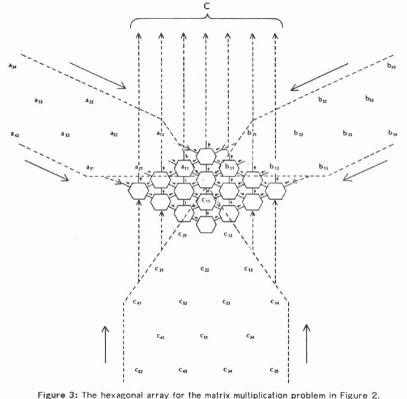
Figure 16: Systolic computation for matrix multiplication on VLSI array. Reproduced from  [24, Fig. 3].

Appendix E Acknowledgments

I thank Katherine Yelick for motivating the central question of this paper, and James Demmel and members of the BeBOP group at UC Berkeley, including Evangelos Georganas, Penporn Koanantakool and Nicholas Knight, for patiently listening to several iterations of these ideas. I thank Joseph Landsberg whose course inspired this line of thought. I thank Niranjini Rajagopal for comments on the draft. This work is funded by the U.S. Department of Energy, Office of Science, Office of Advanced Scientific Computing Research, Applied Mathematics and Computer Science programs under contract No. DE-AC02-05CH11231, through the Dynamic Exascale Global Address Space (DEGAS) programming environments project.

References

• [1] S.Β Agmon. Lecture about Mackey functors, 2012.
• [2] B.Β Alpern, L.Β Carter, and J.Β Ferrante. Modeling parallel computers as memory hierarchies. In Programming Models for Massively Parallel Computers, 1993.
• [3] C.Β Ancourt and F.Β Irigoin. Scanning polyhedra with do loops. In PPoPP, PPoPP ’91, pages 39–50, New York, NY, USA, 1991. ACM.
• [4] G.Β Bilardi, A.Β Pietracaprina, G.Β Pucci, M.Β Scquizzato, and F.Β Silvestri. Network-oblivious algorithms. CoRR, abs/1404.3318, 2014.
• [5] G.Β E. Blelloch, J.Β T. Fineman, P.Β B. Gibbons, and H.Β V. Simhadri. Scheduling irregular parallel computations on hierarchical caches. In SPAA, 2011.
• [6] G.Β E. Blelloch, P.Β B. Gibbons, and H.Β V. Simhadri. Low-depth cache oblivious algorithms. In SPAA, 2010.
• [7] L.Β E. Cannon. A Cellular Computer to Implement the Kalman Filter Algorithm. PhD thesis, Montana State University, Bozeman, MT, USA, 1969. AAI7010025.
• [8] B.Β L. Chamberlain, E.Β C. Lewis, and L.Β Snyder. Problem space promotion and its evaluation as a technique for efficient parallel computation. In ICS, 1999.
• [9] R.Β A. Chowdhury and V.Β Ramachandran. The cache-oblivious gaussian elimination paradigm: theoretical framework, parallelization and experimental evaluation. In SPAA, 2007.
• [10] R.Β A. Chowdhury, V.Β Ramachandran, F.Β Silvestri, and B.Β Blakeley. Oblivious algorithms for multicores and networks of processors. JPDC, 73(7), 2013.
• [11] M.Β Christ, J.Β Demmel, N.Β Knight, T.Β Scanlon, and K.Β A. Yelick. Communication lower bounds and optimal algorithms for programs that reference arrays - part 1. Technical Report UCB/EECS-2013-61, UC Berkeley, 2013.
• [12] A.Β Darte, R.Β Schreiber, and G.Β Villard. Lattice-based memory allocation. IEEE Trans. Comput., 54(10):1242–1257, Oct. 2005.
• [13] P.Β Feautrier. Parametric integer programming. RAIRO - Operations Research - Recherche OpΓ©rationnelle, 22(3):243–268, 1988.
• [14] P.Β Feautrier. Some efficient solutions to the affine scheduling problem. part ii. multidimensional time. International Journal of Parallel Programming, 21(6):389–420, 1992.
• [15] P.Β Feautrier. Automatic parallelization in the polytope model. In G.-R. Perrin and A.Β Darte, editors, The Data Parallel Programming Model, volume 1132 of LNCS, pages 79–103. Springer Berlin Heidelberg, 1996.
• [16] M.Β Frigo, C.Β E. Leiserson, H.Β Prokop, and S.Β Ramachandran. Cache-oblivious algorithms. In FOCS, 1999.
• [17] The GAPΒ Group. GAP – Groups, Algorithms, and Programming, Version 4.7.6, 2014.
• [18] M.Β Griebl. Automatic Parallelization of Loop Programs for Distributed Memory Architectures. University of Passau, 2004. habilitation thesis.
• [19] P.Β Husbands and K.Β Yelick. Multi-threading and one-sided communication in parallel lu factorization. SC ’07, pages 31:1–31:10, New York, NY, USA, 2007. ACM.
• [20] D.Β Irony, S.Β Toledo, and A.Β Tiskin. Communication lower bounds for distributed-memory matrix multiplication. JPDC, 64(9):1017–1026, Sept. 2004.
• [21] R.Β M. Karp, R.Β E. Miller, and S.Β Winograd. The organization of computations for uniform recurrence equations. J. ACM, 14(3):563–590, July 1967.
• [22] P.Β Koanantakool and K.Β Yelick. A computation- and communication-optimal parallel direct 3-body algorithm. SC ’14, pages 363–374. IEEE Press, 2014.
• [23] H.Β Kung and W.-S.Β T. Lin. An algebra for VLSI algorithm design. Technical report, Computer Science Department, Carnegie Mellon University, 1983.
• [24] H.Β T. Kung. Let’s design algorithms for VLSI systems. In Proceedings of the Caltech Conference On VLSI, pages 65–90. California Institute of Technology, 1979.
• [25] L.Β Lamport. The parallel execution of do loops. Commun. ACM, 17(2):83–93, Feb. 1974.
• [26] S.Β Lang. Algebra, volume 211 of Graduate Texts in Mathematics. Springer, 2002.
• [27] V.Β Lefebvre and P.Β Feautrier. Automatic storage management for parallel programs. Parallel Comput., 24(3-4):649–671, May 1998.
• [28] F.Β T. Leighton. Introduction to parallel algorithms and architectures: array, trees, hypercubes. Morgan Kaufmann Publishers Inc., San Francisco, CA, USA, 1992.
• [29] C.Β E. Leiserson. Fat-Trees: Universal networks for hardware-efficient supercomputing. IEEE Transactions on Computers, C–34(10), 1985.
• [30] C.Β Lengauer. Loop parallelization in the polytope model. In E.Β Best, editor, CONCUR’93, volume 715 of LNCS, pages 398–416. Springer Berlin Heidelberg, 1993.
• [31] M.Β W. Liebeck, C.Β E. Praeger, and J.Β Saxl. On the O’Nan-Scott theorem for finite primitive permutation groups. Journal of the Australian Mathematical Society (Series A), 44:389–396, 6 1988.
• [32] A.Β W. Lim and M.Β S. Lam. Maximizing parallelism and minimizing synchronization with affine transforms. POPL ’97, pages 201–214, New York, NY, USA, 1997. ACM.
• [33] D.Β Moldovan. On the analysis and synthesis of vlsi algorithms. IEEE Transactions on Computers, 31(11):1121–1126, 1982.
• [34] F.Β QuillerΓ© and S.Β Rajopadhye. Optimizing memory usage in the polyhedral model. ACM Trans. Program. Lang. Syst., 22(5):773–815, Sept. 2000.
• [35] F.Β QuillerΓ©, S.Β Rajopadhye, and D.Β Wilde. Generation of efficient nested loops from polyhedra. Int. J. Parallel Program., 28(5):469–498, Oct. 2000.
• [36] P.Β Quinton. The systematic design of systolic arrays. In Centre National De Recherche Scientifique on Automata Networks in Computer Science: Theory and Applications, pages 229–260. Princeton University Press, 1987.
• [37] H.Β V. Simhadri. Program-Centric Cost Models for Locality and Parallelism. PhD thesis, CMU, 2013.
• [38] E.Β Solomonik and J.Β Demmel. Communication-optimal parallel 2.5D matrix multiplication and LU factorization algorithms. In EuroPar, 2011.
• [39] M.Β E. Wolf and M.Β S. Lam. A data locality optimizing algorithm. In PLDI, PLDI ’91, pages 30–44, New York, NY, USA, 1991. ACM.
• [40] M.Β E. Wolf and M.Β S. Lam. A loop transformation theory and an algorithm to maximize parallelism. IEEE Trans. Parallel Distrib. Syst., 2(4):452–471, Oct. 1991.