Reinforcement Control with Hierarchical Backpropagated Adaptive Critics

Abstract

Present incremental learning methods are limited in the ability to achieve reliable credit assignment over a large number time steps (or events). However, this situation is typical for cases where the dynamical system to be controlled requires relatively frequent control updates in order to maintain stability or robustness yet has some action/consequences which must be established over relatively long periods of time. To address this problem, the learning capabilities of a control architecture comprised of two Backpropagated Adaptive Critics (BAC’s) in a two-level hierarchy with continuous actions are explored. The high-level BAC updates less frequently than the low-level BAC and controls the latter to some degree. The response of the low-level to high-level signals can either be determined a priori or it can emerge during learning. A general approach called Response Induction Learning is introduced to address the latter case.

1 Introduction

There has recently been considerable interest in the application of reinforcement learning methods to problems of adaptive (or intelligent) control. Perhaps the most recognized early work on this subject is a 1983 paper by Barto, Sutton, and Anderson  [1] which demonstrated stabilization of the oft-studied cart-pole problem (see Figure 2). In this paper the authors introduced the “adaptive heuristic critic,” the function of which is to evaluate the current state in terms of expected future (cumulative) reinforcements. Sutton’s work on temporal differences  [5] refined these notions, and extended their application to nonlinear feedforward neural networks. His work is the basis for the present “critic network,” the goal of which is to estimate the sum of future reinforcements ($p_{t}$):

$$p_{t}\ =\ \sum_{k=0}^{\infty}\gamma^{k}r_{t+k+1},$$ (1)

where $r_{t+k+1}$ is the reinforcement received at time $t+k+1$ and $\gamma$ is the discount factor ($0<\gamma<1$). Note that the closer the discount factor is to one the greater the “foresight” of the critic, i.e., the more future reinforcements should incorporated in the current prediction.

For many applications, in order to achieve dynamic stability and control efficacy the interval between controller updates are likely to be small compared to the time between some actions and their consequences, especially for more difficult “intelligent” control problems. However, the greater the number of time steps between initial states and goal states, the more difficult it is to achieve reliable credit assignment for actions which incurred early on, i.e., the more “foresight” required by the critic. A reasonable solution is to have motion primitives which require control actions to “steer” them in some way. These steering commands would occur less frequently than the motor commands issued by the primitives. Watkins  [13] presented an interesting paradigm for hierarchical control based on ship navigation which has several parallels to, the present work. This idea is also similar to the principle of “cascade control” developed for process control.

In this paper a simple two-level hierarchy of reinforcement learning modules is implemented in such a way that the “low level” module controls the actuators directly and is rewarded for maintaining stability while the “high level” module steers the low level module in order to maximize longer term positive reinforcement. Two cases are considered: one in which the role of the steering command is predefined in terms of the reinforcement to the low level controller, and the much more difficult cases where the role is not defined a priori but is developed as learning progresses.

2 The Backpropagated Adaptive Critic (BAC)

2.1 Background

In the Barto etal. work discussed in the last section, the state space of the plant was broken up into “boxes” and the control actions were binary. While their results were impressive, the discrete nature of the method is impractical for problems which either require high fidelity control or which have a high dimensional state space. Nevertheless, they achieved stabilization of the cart-pole system within seventy trials on average—considerably better than any of the continuous approaches appearing in the literature (or here).

Anderson  [4] later used critic and action modules based on backpropagated multilayer perceptrons for stabilization of the cart-pole problem. Although inputs to the modules were continuous, the associative learning method for training the action network still required (stochastic) binary actions. Around 8,000 trials were required on average to stabilize the system. Note that a “trial” starts with the cart and pole randomly within the state space ends when the position of either exceed its bounds.

Werbos  [2, 3] introduced an architecture called the Backpropagated Adaptive Critic (BAC) for which a utility function similar to a critic is used as a guide for training the action module. In this approach continuous inputs and actions are allowed. Jordan and Jacobs  [12] and Jameson  [11] provided some of the first results with this approach, and both studied the cart-pole problem. Results for these cases are presented in Table 1 (and shall be discussed further).

2.2 Architecture: Indirect BAC

A schematic of the BAC is shown in Fig. 1, and consists of three networks: the action, model, and critic networks, indicated by the letters “A,” “M,” and “C,” respectively. This architecture, for reasons to be explained shortly, is called the Indirect BAC. For a more detailed description of this architecture, see  [11, 3]. Note that arrows crossing the left border of the BAC in Fig. 1 correspond to signals to and from the same BAC but for the previous time step, and similarly arrows that cross the right border refer to the next time step. Dashed lines represent feedback errors which may pass through a network with or without affecting its weights; if a dashed line is visible inside the network block the weights are not affected, otherwise they are.

For the experiments discussed below all the networks contained a single hidden layer with (seven) Gaussian activation functions and an output layer with linear activation functions.

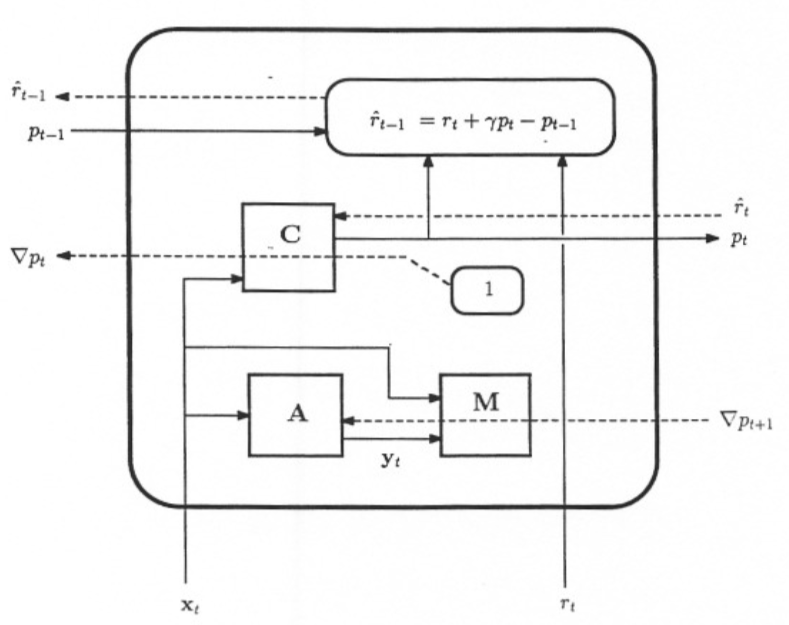
Figure 1: BAC for one time step

The model network performs system identification. In the preferred form, it predicts the change in state $\Delta x$ as a function of the current state and action, i.e., its weights are adapted to minimize, for all times,

$$k_{m}\ (\Delta x\ -\ \Delta x_{pred}),$$ (2)

where $\Delta x_{pred}$ is the output of the model network, and $k_{m}$ is a scaling factor; the feedback path for training the model network is not shown in Fig. 1. Training of this network is best achieved before training the controller by starting the system in a random place in the state space and letting the system evolve with random actions. After this network has adapted satisfactory, its weights are frozen.

From eq. 1 it is easy to show that if the critic predictions are correct then $p_{t}=r_{t+1}+\gamma p_{t}$. Hence, for training the critic, if $r_{t+1}+\gamma p_{t}$ is the target and $p_{t}$ the actual output, then the critic error is:

$$\hat{r}_{t}\equiv r_{t+1}+\gamma p_{t+1}-p_{t},$$ (3)

which corresponds to the following equation for changing the weights of the critic network (see  [5] for further clarification):

$$\Delta{\bf w}_{c,t}=\eta\ {\hat{r}}_{t+1}{\bf\nabla}p_{t}\quad+\quad\hbox{momentum},$$ (4)

where ${\bf w}_{c,t}$ is the weight vector for the critic network, $\eta$ is the learning rate, and ${\bf\nabla}p_{t}$ is the gradient of $p_{t}$ with respect to the weights.

The action (controller) network determines which action ${\bf y}_{t}$ to take as a function of the current state ${\bf x}_{t}$ (note that in general ${\bf y}_{t}$ is a vector, but for the cart-pole problem it is just a scalar quantity).

To adapt the action network in order to increase $p_{t}$, a path is needed from the critic network to the action network in order to feed back the gradient of $p_{t}$. However, since the critic output is a function only of the state (${\bf x}_{t}$), the model network is needed to provide a feedback pathway to the action network. Note that the gradient of $p_{t}$ corresponds to a “error signal” of one (1) at the output of the critic. In order to establish more accurate gradients (and enhance robustness) a small Gaussian noise component is added to the outputs of the action network. However, feedback is performed with activities corresponding to zero noise (see  [3]).

2.3 Direct BAC Architecture

Another form of the BAC, called the “Direct BAC,” is virtually the same as the BAC just described except that the critic input consists of the current state and action—no model network is needed. For this case the action is included as input to the critic network.

3 Single Level BAC Control with the Cart-Pole Problem

3.1 The Cart-pole System

The cart-pole system, studied extensively in the literature in connection with reinforcement learning, is shown in the Fig. 2. The state of this system is completely described by four quantities which comprise the state vector ${\bf x}_{t}$: the position and velocity of the cart, and angular position and rate of the pole. The goal is to keep the inverted pole balanced and the cart from hitting either end of the track by controlling the force (proportional to $y_{t}$) exerted on the cart. The equations of motion of the system are:

$$\ddot{x}\ = \ {{f_{c}\ +\ m_{p}L\left[\dot{\theta}^{2}\sin\theta\ -\ \ddot{\theta}\cos\theta\right]}\over m_{c}\ +\ m_{p}}$$ (5)

$$\ddot{\theta}\ = \ {g\sin\theta\ +\ \cos\theta\left[{-f_{c}\ -\ m_{p}L\dot{\theta}^{2}\sin\theta\over m_{c}+m_{p}}\right]\over L\left[{4\over 3}\ -\ {m_{p}\cos^{2}\theta\over m_{c}+m_{p}}\right]}$$ (6)

where,

$$m_{c}\ \ = \ \ 1.0\,kg\ \ =\ \ \hbox{mass of the cart}$$

$$m_{p}\ \ = \ \ 0.1\,kg\ \ =\ \ \hbox{mass of the pole}$$

$$L\ \ = \ \ 1.0\,m\ \ =\ \ \hbox{(nominal) length of the pole}$$

$$g\ \ = \ \ 9.8\,m/s^{2}\ \ =\ \ \hbox{acceleration of gravity}$$

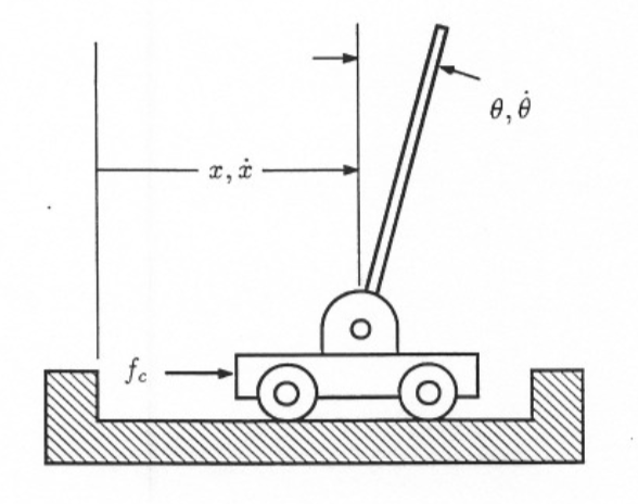
Figure 2: The cart-pole system

The external reinforcement signal ($r$) used for the experiments was:

$$r\ =\ \sqrt{\left({\theta\over\theta_{r}}\right)^{2}\ +\ \left({x\over x_{r}}\right)^{2}},$$ (7)

where $\theta_{r}=12^{\small o}$ and $x_{r}=2.4$m are the ranges of the motion allowed for the pole angle and cart position, respectively; if either range is exceeded, a new trial begins. Note that I generally found the learning to be roughly half as fast if the system was failure driven, i.e., $r=-1$ when a failure occurs, or $r=0$ otherwise (see  [11] for more detailed performance comparisons).

To balance the pole it is necessary to have this force adjusted fairly frequently. However, the gross motion of the cart depends on the short-term averaged angle of the pole; if it is generally tilted to the right the cart will slowly accelerate to the right (actually, a small oscillatory motion which keeps the pole balanced will be superimposed on this acceleration—note that if the pole is “balanced” at a constant angle $\theta_{b}$, the acceleration of the cart is $\ddot{x}=g\tan\theta_{b}$). The point is that the time constant of this gross motion of the cart is much longer than that of the pole. In other words, this problem requires strong critic foresight in order to keep the cart centered. This fact motivated me to perform similar experiments as my earlier paper  [11] but with a slower servo rate, i.e., all other parameters were kept constant except for the servo rate.

3.2 Results for the Single-Level BAC with Different Servo Rates

The results of these experiments are presented in Table 1. An experiment consisted of letting the BAC learn until it either stabilized the system (called a “success” in Table 1) or until the number of trials reached 1,200 (or 3,000 for the Direct BAC), constituting a “failure.” The parameters for all the experiments the (except case 4) were identical; the learning rates for the action and critic networks were .01 and .02, respectively. The model network was trained in each case for 1,000 time steps.

TABLE 1
Experimental Results for the Cart-Pole with
Single-Level Adaptive Critic Architectures
Case	Architecture	servo rate	$(SR)^{a}$	$(N_{\hbox{\it ave}})^{b}$	$(M_{\hbox{\it ave}})^{c}$
		(hz)
1	Indirect BAC	50	6/30	860	110,000
2	Indirect BAC	25	15/30	686	47,500
3	Indirect BAC	17	14/30	760	35,500
4	Direct BACd	50	18/20	$\approx 20,000$	NA
5	Direct BAC	25	3/10	2,300	380,000
6	Direct BAC	17	11/30	1,100	120,000
${}^{a}(SR)$ = (no. of successes)/(no. of experiments)
${}^{b}(N_{\hbox{\it ave}})$ = Average no. of trials prior to success
${}^{c}(M_{\hbox{\it ave}})$ = Average no. of time steps prior to successful trial
dfrom Jordan and Jacobs  [12]

The results in Table 1 show that both BAC’s (Indirect and Direct) had superior performance for the faster servo rates. This was mostly likely for the following reason: although the shortened pole is harder to balance for a slower servo rate (the gains must be more finely tuned), less foresight is required from the critic to center the cart.

The data for case 4 in Table 1 was obtained from Jordan and Jacobs  [12], who used an architecture very similar to the Direct BAC but with a different reinforcement signal (related to the time to failure). However, whereas the criteria for a “success” was 20,000 time steps for other cases in Table 1, only 1,000 time steps qualified as a success in Jordan and Jacobs paper.

Note that the control logic involved in stabilizing the cart-pole system is not very complicated. The main problem seems to be the long time constant of the cart’s motion. The results of Table 1 strongly corroborate this hypothesis.

4 The Two-Level BAC with Explicit Low-level Role

Put most simply, the principle of the two-level BAC is this: use a low-level ($\cal LL\$) BAC with a fast servo rate to directly control the actuators for short term stability, and a high-level ($\cal HL\$) BAC with a slower servo rate to control the $\cal LL\$BAC to maximize the (long term) reinforcement.

The preferred form of the two-level BAC is shown in Fig. 3. Only one $\cal HL\$BAC and one $\cal LL\$BAC are used in this architecture. The $\cal HL\$BAC updates once for every N $\cal LL\$BAC updates, where N was 40 for the simulations below.

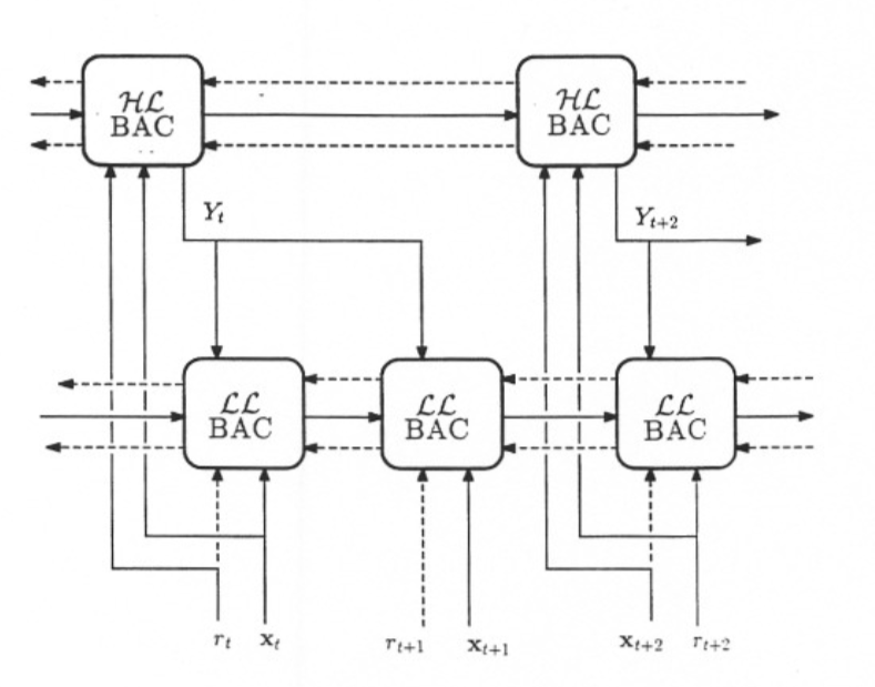
Figure 3: Schematic of the Two-Level BAC

The $\cal HL\$BAC is virtually identical to the “standard” BAC shown in Fig. 2, except the $\cal HL\$action, ${\bf Y}_{t}$, is used as part of the input to the $\cal LL\$instead of determining the force on the cart. ${\bf Y}_{t}$ is referred to as the “plan”; in general it can be a vector, but for examples in this paper it is just a scalar quantity. Note that the $\cal HL\$receives the usual reinforcement from the environment.

Fig. 4 shows the architecture of the $\cal LL\$BAC, which has the reinforcement signal

$$r^{\prime}_{t}=(Y_{t-L}-\theta_{t})^{2}$$ (8)

where $\theta_{t}$ is the angle of the pole from top center, and $L$ is the number of elapsed time steps since the last $\cal HL\$update. In other words, the $\cal LL\$controller learns to perform actions (forces on the cart) that keep the pole at an angle equal to the plan input. Note that the $\cal HL\$action, $Y$, is input to the $\cal LL\$action and critic networks.

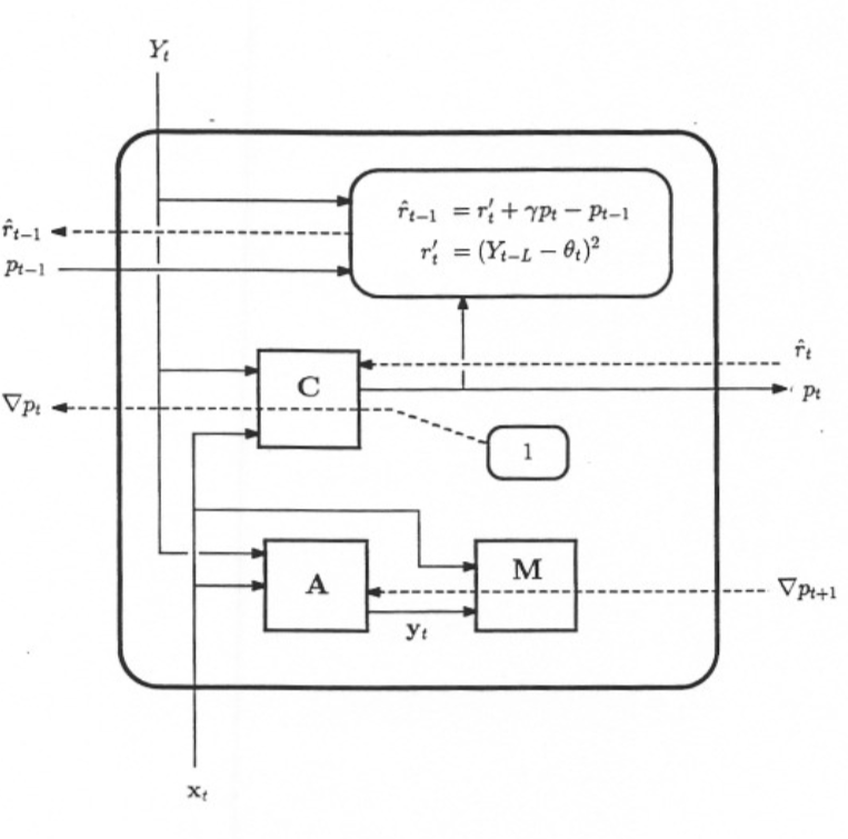
Figure 4: Schematic of the Low-Level BAC (with explicit function)

It is most desirable that the environment of each BAC have the Markov property, i.e., that future states and reinforcement signals depend only on the current state and action(s). As Watkins pointed out  [13], if the $\cal LL\$controller is subject to state transitions that are not entirely caused by its own actions then the Markov property does not hold for the $\cal LL\$controller. However, the case here is a little more subtle. Suppose that, instead of predicting the value of the cumulative reinforcement ($p$), the $\cal LL\$critic predicted just $r$ for the next time step (this is equivalent to predicting p for $\gamma=0$). Since the $\cal LL\$critic has no way of knowing whether $Y$ is going to change on the next time step, it would do a poor job of predicting $r$ since the latter depends on $Y$. However, because $Y$ does stay constant for many ($N$) $\cal LL\$time steps between each change in its value, the $\cal LL\$critic s prediction would be somewhere in the “ball park;” it would tend to yield a short term average of the oncoming values of $r$. The fact that an accumulation of $r$ is predicted rather than just $r$ significantly mitigates the prediction difficulty because of the averaging effect of the accumulation.

It was found for the simulations described below that the $\cal LL\$controller failed to work if the $\cal HL\$action was not included in the $\cal LL\$critic input space. Otherwise the $\cal LL\$learned to control the pole angle reliably.

Note that the $\cal LL\$model network does not require the $\cal HL\$action as part of its input. This would not be the case, however, if the high level actions affected the cart-pole system through some other channel than the low level controller, such as through additional forces on the cart.

The single-level Indirect BAC (of the previous section) works best with two phases of learning—the model network is trained in the first phase for random actions, then the action network is trained via the feedback from the critic. A similar situation occurs for the two-level BAC except that two phases are utilized for each level. The phases are reiterated below for clarity.

  Phase I:

The $\cal LL\$model network learns to predict the change in state for random $\cal LL\$actions over time step. The $\cal LL\$action weights are then frozen.

  Phase II:

The $\cal LL\$action network learns to balance the pole angle at an angle proportional to the $\cal HL\$action (plan) for random values of the latter. The $\cal LL\$action weights are then frozen.

  Phase III:

The $\cal HL\$model network is trained to predict the change in state for random $\cal HL\$actions N time steps ahead. The $\cal HL\$model weights are then frozen.

  Phase IV:

The $\cal HL\$action network learns to keep the cart centered.

For the two-level Direct BAC only two phases of learning are required, where phases I and II for the Direct BAC correspond to phases II and IV for the Indirect BAC, respectively.

4.1 Experimental Results

Table 2 presents results obtained for the cart-pole system with a servo rate of 50 hz—corresponding to the most difficult of the cases presented in Table 1. Note that the performance of the $\cal HL\$controller in phase IV learning was virtually identical to the performance of the system described in  [11], where a proportional derivative control loop essentially fulfilled the role of the $\cal LL\$controller in the present example. The learning performance in phases I through III was very reliable, i.e., no local minima were encountered over the ten experiments.

TABLE 2 Results for Two-Level BAC Architectures with Explicit Low-Level Function over Ten Experiments (50 hz Servo Rate)
Architecture	Phase	Typical No. of Trials	Average No. of Time Steps
Indirect BAC	I	800	10,000
” ” ”	II	900	130,000
” ” ”	III	400	150,000
” ” ”	IV	160	10,000
Direct BAC	I	1,600	650,000
” ” ”	II	450	50,000

One way to make a direct comparison between the results shown in Table 2 for the two-level BAC with the corresponding single-level BAC (for the 50 hz servo rate) is to compare the total number of time steps prior to success. This yields 300,000 steps for the two-level BAC and 360,000 steps for the single-level BAC (10,000 steps are included in the latter to account for phase I learning—which is not included in Table 1). However, of the thirty experiments in Table 1, only six succeeded, whereas the success ratio for the two-level BAC was much greater (nine successes out of ten experiments for phase IV and no failures in the prior phases).

Given the additional complexity associated with the model network, a reasonable conclusion might be that having a model is not worth the effort for a two-level BAC. For the cart-pole problem this might be the case. However, it seems likely that there are many problems where a Direct BAC would be inadequate for a given single level of control. In fact, the single-level BAC experiments of Table 1 indicate that the Indirect BAC was far inferior to the Direct BAC for the 50 hz servo rate.

5 Response Induction (RI) Learning

What happens if, instead of forcing the pole to “follow” the $\cal HL\$plan through an internal $\cal LL\$reinforcement, the $\cal LL\$controller is provided the same (external) reinforcement as the $\cal HL\$? What role does the $\cal HL\$plan, with its influence on the $\cal LL\$controller, take on for this case, i.e., what “subtask” does the $\cal LL\$controller learn? I generally found that, given enough time, the effects of the $\cal HL\$plans on the $\cal LL\$actions became negligible. Since there was no inclusion of the plans in the reinforcement provided to the $\cal LL\$controller, the plans became disturbances to be rejected.

One way to induce the $\cal LL\$to learn to react to the $\cal HL\$plan signals without expressing explicitly how to react to them is to affect the weights of the action network such that each

$$\delta_{i}\ \equiv\ {\partial p\over\partial Y_{i}},\quad\forall\ i\in{\cal P}$$ (9)

is some significant positive value, where $p$ is the $\cal LL\$critic output (see eq. 1), $Y_{i}$ is the $ith$ $\cal HL\$plan input, and ${\cal P}$ is the set of units in the $\cal LL\$action network corresponding to the plan inputs; note that The term “$\delta$” is used in the same sense as Rumelhart etal.  [9], Vol. 1, Chapter 8, with respect to backpropagation. Again, for this case the $\cal LL\$BAC receives the same reinforcement signal from the environment as the $\cal HL\$BAC.

Perhaps the more obvious approach for inducing a response would be to replace $\partial p/\partial Y_{j}$ with $\partial y_{i}/\partial Y_{j}$ in eq. 9, where $y_{i}$ and $Y_{j}$ correspond to the $ith$ and $jth$ $\cal LL\$and $\cal HL\$action signals, respectively. Yet this was found experimentally to be much less effective. The disturbing effect of the response induction usually kept the $\cal LL\$BAC from keeping the system stable for any appreciable amount of time. This was probably because response induction based on the action network output requires an immediate effect, whereas the induction based on the critic output elicits a response which can be mitigated over several time steps (since the critic output reflects present and future events). It is fortuitous that most of the factors for critic-based RI learning are already computed during $\cal LL\$action network learning.

To see how the $\cal LL\$action network weights are adapted to increase $\delta_{i}$ (for $i\in{\cal P}$), consider the following error functon for the output of the $\cal LL\$action network:

$$E\ =\ -E_{\hbox{\scriptsize\it critic}}\ +\ E_{\hbox{\scriptsize\it influence}},$$ (10)

where

$$E_{\hbox{\scriptsize\it influence}}\ =\ -{k_{1}\over n_{p}}\ \sum_{i\in{\cal P}}e^{-\delta^{2}_{i}/k^{2}_{2}},$$ (11)

where ${\cal P}$ is the set of input units corresponding to the plan inputs, $E_{\hbox{\scriptsize\it influence}}$ is the “influence error,” and $E_{\hbox{\scriptsize\it critic}}$ is the effective error of the $\cal LL\$action output due to feedback from the critic network (during phase II learning for the two-level Indirect BAC or phase I learning for the two-level Direct BAC). The weights of the $\cal LL\$action network are adapted such as to maximize $E$ in eq. 10. The constant $k_{1}$ determines the maximal degree of the plan s influence and the constant $k_{2}$ determines the rate at which the influence is induced (I generally obtained adequate results with $k_{2}=k_{1}/2$; note that if $k_{2}$ is set too large the maximal induction, $\delta_{i}\approx k_{1}$, will not be achieved).

For the experiments, the weight of each connection between units in the hidden layer to the (single) plan input unit was adjusted an amount proportional to $\partial E/\partial w_{ji}$ (the rest were adjusted normally):

$$\Delta w_{ji}\ =\ \eta\left[\delta_{j}Y_{i}\ +\ k_{1}\,k_{2}\,\delta_{i}\delta_{j}\,e^{-\delta^{2}_{i}/k^{2}_{2}}\right]\ +\ \hbox{momentum},$$ (12)

where $\eta$ is the learning rate, $w_{ji}$ is the weight connecting the $jth$ hidden unit to the $ith$ input unit (the plan unit), and $\delta_{j}$ corresponds to the $jth$ hidden unit and is defined in the manner of Rumelhart etal.

With the approach just described the $\cal LL\$action network essentially learns to maximize its reinforcement while responding in some fashion to the $\cal HL\$plans (which changes every $N$ $\cal LL\$time steps). Experiments with the cart-pole system revealed that the $\cal LL\$action network reliably produced smooth and significant responses to the $\cal HL\$plans while keeping the pole balanced. At the very beginning of the $\cal LL\$BAC learning $\delta_{i}$ was typically small, and hence the rate of the response induction was small because operation was in the central (flatter) region of the Gaussian “bowl.” This allowed the system to achieve reasonable stability before stronger responses to the $\cal HL\$actions were induced.

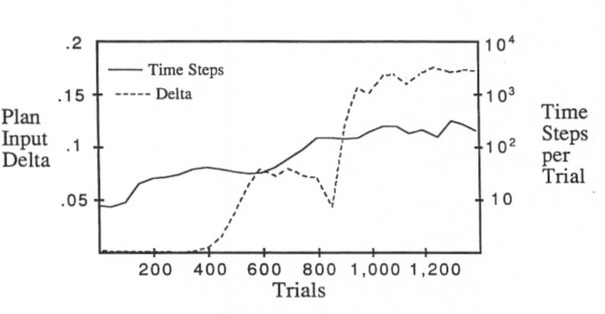
Figure 5: Plot of ($\delta_{i}$) and the number of steps/trial versus the number of trials

Figure 5 shows the evolution of $\delta_{i}$ for three typical experiments during phase II two-level Indirect BAC learning; note that $i=5$, i.e., the first four inputs to the action network were the state variables, and the fifth was the single plan input. Both curves were smoothed by averaging the steps per trial (and the $\delta_{i}$) into bins of 50 trials. This plot shows how the response induction occurs after moderate stability of the system has been achieved.

I have ignored so far the implications of RI learning for case when the plan input has more than one component. For this case, it is desirable that the response trajectory due to each plan component be different than the response trajectories due to the remaining plan components, i.e., that the same response trajectory for one plan component value cannot be achieved for some value of another plan component. The fact that the plan components vary independently with respect to each other during RI learning does not guarantee that the trajectories of the responses will be be different, although it seems highly likely that they will be somewhat different. Finding methods which enhance the diversity of the response trajectories is certainly one area for future research.

5.1 Experimental Results with RI Learning

During the experiments it was usually the case that a change in the plan input caused a fairly rapid shift in the pole angle, after which the pole moved smoothly from the new (shifted) position, usually in the direction from which it started. In several experiments, however, the $\cal LL\$was observed to balance the pole at an angle proportional to the plan signal, just as in the more supervised case in Sec. 1.

After performing some degree of (RI) parameter optimization, I performed fifteen experiments using RI learning during phase II for the two-level Indirect BAC; all other parameters were identical to those used for obtaining the results given in Table 2. During phase II RI learning learning and phase III $\cal HL\$model learning, uniformly random $\cal HL\$actions in the ranges [-.3, .3] and [-.7, .7], respectively, were provided to the $\cal LL\$BAC. The values of $k_{1}$ and $k_{2}$ were .35 and .14, respectively.

Over these fifteen experiments, the average number of trials/(time steps) deemed adequate for phase II RI learning learning was 1,300/190,000. The average number of trials/(time steps) deemed adequate for phase III ($\cal HL\$model) learning was 1,000/140,000. For phase IV learning, five of the experiments resulted in finding a solution within 700 trials (otherwise the experiment was halted). The average number of trials/(time steps) for the solutions was 470/25,000.

A common problem observed during the (ten) failures was that the state space was covered insufficiently during RI learning. This problem was tacitly eliminated for the explicit role case of the previous section in that the corresponding response did cover the solution space, i.e., the random plan signals corresponded to random pole angles, distributed around its top center position.

5.2 Outlook on RI Learning

Inducing the $\cal LL\$action network simply to react to the plan signals while maximizing its local reinforcement seems crude in the sense that the type of reaction learned may not necessarily be useful for $\cal HL\$performance. However, because it is so general it lends considerable leeway to the $\cal LL\$action network for reinforcement maximization. This leeway could be utilized most effectively, perhaps, by augmenting the “environmental” reinforcement signal with terms related to such factors as state space exploration and/or to trajectory smoothing. It may be useful to construct separate critics solely for the purpose of response induction, letting a new critic respond to some of the factors just mentioned. In any case, for most applications it seems most desirable that the $\cal LL\$behavior with respect to $\cal HL\$actions be deterministic, and that the state space is adequately covered.

6 Role Learning Based on Time Constant Identification

Another potential way to induce useful $\cal LL\$role emergence is more directly related to the “explicit function” learning in Sec. 3. This would be to have the intelligent controller figure out itself which components of the plant’s state variables are “slow” and which are “fast” and apportion control appropriately (e.g., as the control was apportioned in Sec. 3). This would not be as general as RI learning in that specific state variables must be identified and routed to different levels of control, whereas in RI learning different functions of the state variables may implicitly be routed. However, it seems like this might be more practical than RI learning for the near term.

7 Conclusion

In this paper I have addressed the problem of extending the time span over which causes and effects can be accounted for reliably by a Backpropagated Adaptive Critic. The general ideas, of course, are applicable to other incremental learning methods (e.g., the feedback in time method  [8]).

The functional allocation within the hierarchical architecture has been approached from two extremes: in single case, Explicit Role Learning (ERL), the role of the low level controller is predefined based on knowledge of the system, and in the other case, Response Induction Learning (RIL), no knowledge and very little structure is imbedded in the architecture.

Results for the two-level BAC with ERL show that it is considerably more reliable than a corresponding single-level BAC for the cart-pole problem, although at a cost of more user interaction. It is likely that the model and action/critic learning phases within each BAC level can be meshed together in a form of learning that has attributes of both of the original (different) phases. This is certainly one area for future work (for single-level Indirect BAC learning as well as the hierarchical case). Elimination of the phases related to separate learning for the low and high level BAC’s seems to be fundamentally much more difficult because of the desirability of surrounding each BAC (level) with a stationary environment. Perhaps the most promise lies in providing mechanisms for automatically detecting when to switch these phases, rather than finding ways to eliminate the phases themselves.

RIL was introduced as an example of how the emergence of functional roles might be achieved within a hierarchical (reinforcement) control system. The method is very reliable at inducing responses while allowing the controller to “mind” the reinforcement signals. However, such responses, while usually quite deterministic, were not always conducive to solving the problem. However, the generality of the method leaves room for many varieties of enhancement.

The extension of the present approach to more than two levels of control seems straightforward in principle. For this case, the servo rates of each level would be progressively slower as the hierarchy is ascended, and each level would control the level beneath it. Also, the present discussion has also been limited to cases where control signals are issued at equal time intervals. The extension to intermittent control is another important area for future research.

Is this hierarchical BAC approach valid for more challenging problems than the cart-pole system? The difficulty with the latter seems not to be with the control logic required (which is fairly simple), but rather with the widely differing time constants of the motion of the cart and pole, a hypothesis which is strongly corroborated by results in Table 1. It is likely that a single-level BAC can learn much more (logically) difficult problems than the cart-pole as long as causes and effects occur within reasonable time spans. The multi-level BAC is just a way of extending the performance when large differences in time constants are present, whether the “logical” problem addressed within each level is difficult or not.

I

References

- [1] Barto, A. G., Sutton, R. S., and Anderson, C. W. (1983), Neuronlike Elements That Can Solve Difficult Control Problems, IEEE Trans. on Systems, Man, and Cybernetics, 13, 835-846.
- [2] Werbos, P. J. (1989), Beyond Regression, New Tools for Prediction and Analysis in the Behavioral Sciences, Ph.D. Thesis, Harvard University, Nov. 1974, Cambridge, MA.
- [3] Werbos, P. J. (1990), A Menu of Designs for Reinforcement Learning Over Time, Neural Networks for Control, MIT Press.
- [4] Anderson, C. W. (1988), Strategy Learning with Multilayer Connectionist Representations, Tech. Report TR87-509.3, G. T. E. Laboratories.
- [5] Sutton, R. S. (1988), Learning to Predict by the Methods of Temporal Differences, Machine Learning, 3, 9-44.
- [6] Sutton, R. S. (1984), Temporal Credit Assignment in Reinforcement Learning, Ph.D. Thesis, Dept. of Computer and Information Sciences, Univ. of Mass., Amherst.
- [7] Sutton, R. S.(1990), Integrated Architectures for Learning, Planning, and Reacting Based on Approximating Dynamic Programming,” Proc. 7th Int. Conf. on Machine Learning.
- [8] Nguyen, D., and Widrow, B. (1989), The Truck Backer-Upper: An Example of Self-Learning, Proc. IEEE Int. Conf. on Neural Networks, Washington, D. C., Vol. II, 357-363. I
- [9] Rumelhart, D. E., and McClelland, J. L. (1986), Parallel Distributed Processing: Explorations in the Microstructure of Cognition, Vol. I, MIT Press.
- [10] Sofge, D. A. White, D. A. (1990), Neural Network Based Process Optimization and Control, Proc. 29th Conf. on Decision and Control, Honolulu.
- [11] Jameson, J. W. (1990), A Neurocontroller Based on Model Feedback and the Adaptive Heuristic Critic, Proc. IEEE Int. Conf. on Neural Networks, San Diego, Vol. II, 37-44.
- [12] Jordan, M. I., Jacobs, R. A. (1989), Learning to Control an Unstable System with Forward Modeling. In D. S. Touretzky (Ed.), Advances in Neural Information Processing Systems 2, Morgan Kaufmann.
- [13] Watkins, C. J. (1989), Learning from Delayed Rewards, Ph.D. Thesis, King’s College, Cambridge.
- [14] Miller, W. T. (1989), Real Time Application of Neural Networks for Sensor-Based Control of Robots with Vision, IEEE Trans. on Sys., Man, and Cybernetics, 19, 825-831.
- [15] Schmidhuber, J. H. (1990), Making the World Differentiable: On Using Supervised Learning Fully Recurrent Networks for Dynamic Reinforcement Learning and Planning in Non-Stationary Environments, Report FKI-126-90, Technische Universitat Munchen, Institut fur Informatik, West Germany.