Why Non-equilibrium is Different

Abstract

The 1970 paper, “Decay of the Velocity Correlation Function” [Phys. Rev. ${\bf A1}$, 18 (1970), see also Phys. Rev. Lett. 18, 988, (1967)] by Berni Alder and Tom Wainwright, demonstrated, by means of computer simulations, that the velocity autocorrelation function for a particle in a gas of hard disks decays algebraically in time as $t^{-1},$ and as $t^{-3/2}$ for a gas of hard spheres. These decays appear in non-equilibrium fluids and have no counterpart in fluids in thermodynamic equilibrium. The work of Alder and Wainwright stimulated theorists to find explanations for these “long time tails” using kinetic theory or a mesoscopic mode-coupling theory. This paper has had a profound influence on our understanding of the non-equilibrium properties of fluid systems. Here we discuss the kinetic origins of the long time tails, the microscopic foundations of mode-coupling theory, and the implications of these results for the physics of fluids. We also mention applications of the long time tails and mode-coupling theory to other, seemingly unrelated, fields of physics. We are honored to dedicate this short review to Berni Alder on the occasion of his 90th birthday!

Institute for Physical Science and Technology, University of Maryland, College Park, MD 20742, USA

1 Divergences in Non-equilibrium Virial Expansions

N. N. Bogoliubov[1], by means of functional assumption methods, and later M. S. Green[2] and E. G. D. Cohen[3], using cluster expansion methods, independently solved the outstanding problem in the non-equilibrium statistical mechanics of gases at the time, namely, to extend the Boltzmann transport equation to dense gases as a power series expansion in the density of the gas. These authors were able to formulate a generalized Boltzmann equation for monatomic gases with short ranged central potentials, in the form of a virial expansion of the collision operator whose successive terms involved the dynamics of isolated groups of two, three, four,…, particles interacting amongst themselves. That is the generalized Boltzmann equation was written by these authors as[4, 5]

$$\frac{\partial f({\bf r,{\bf v},t)}}{\partial t}+{\bf v\cdot\nabla_{{\bf r}}}f(({\bf r,{\bf v},t)} = J_{2}(f,f)+J_{3}(f,f,f)+\cdots.$$ (1)

Here $f(({\bf r,{\bf v},t)}$ is the single particle distribution function, for finding particles at position ${\bf r}$ with velocity ${\bf v}$ at time $t.$ The collision operator $J_{2}$ is the usual Boltzmann, binary collision operator, while the $J_{j}$ are collision operators determined by the dynamical events taking place among an isolated group of $j$ particles.

At roughly the same time as the problem of generalizing the Boltzmann equation to higher densities was being addressed, M. S. Green[6, 7] and R. Kubo[8] independently developed a general method for expressing the transport coefficients appearing in the linearized equations of fluid dynamics in terms of time integrals of equilibrium time correlation functions of microscopic currents. These expressions have the general form

$$\xi(n,T) = \int_{0}^{\infty}dt\left\langle j_{\xi}(0)j_{\xi}(t)\right\rangle_{eq}.$$ (2)

Here $\xi(n,T)$ is a transport coefficient such as the coefficient of shear viscosity, thermal conductivity, etc. at fluid density $n$ and temperature, $T,$ the brackets denote an equilibrium ensemble average, and $j_{\xi}(t)$ is the value of an associated microscopic current at some time $t.$ An example that will be important for our discussion is the case of tagged-particle diffusion whereby one particle in a gas of mechanically identical particles has some non-mechanical tag that enables one to follow its diffusion in the gas. For this case, the diffusion coefficient $D$ is given by the Green-Kubo formula:

$$D(n,T) = \int_{0}^{\infty}dt\left\langle v_{x}(0)v_{x}(t)\right\rangle_{eq},$$ (3)

where $v_{x}(t)$ is the $x-$component of the velocity of the tagged particle.

From the density expansion of the collision operator or by an equivalent cluster expansion of the time correlation function expressions, one can, at least in principle, obtain expressions for transport coefficients of the gas as power series in the density, similar to the virial expansions for the equilibrium properties of the same gas. This parallel development indicated the existence of a “super statistical mechanics”. whereby both equilibrium and non-equilibrium properties of a gas can be expressed in the form of virial, or power series, expansions in the density of the gas, obtained by means of almost identical cluster expansion methods. However it quickly became clear that this parallelism was purely illusory, the non-equilibrium properties of a gas have almost nothing in common with its equilibrium properties. The first indication of this situation appeared in 1965 when Dorfman and Cohen[9], among others[10], discovered that almost every term in the non-equilibrium virial expansions diverges!

The differences between the equilibrium and non-equilibrium virial expansions have their origins in the type of correlations upon which the virial coefficients depend. The equilibrium virial coefficients depend only upon static correlations between a fixed number of particles in contrast to the non-equilibrium virial coefficients which depend mainly, if not exclusively, upon dynamical correlations produced by sequences of collisions taking place between a fixed number of particles. To be explicit, the equilibrium virial expansion for the pressure, $p(n,T),$ of a gas at number density $n$ and at temperature $T,$ and the non-equilibrium virial expansion for the transport coefficient, $\xi,$ of a gas at local number density $n$ and at local temperature $T$ are given by

$$\frac{p(n,T)}{nk_{B}T} = 1+nb_{1}(T)+n^{2}b_{2}(T)+\cdots,$$ (4)

$$\frac{\xi(n,T)}{\xi_{0}(T)} = 1+n\sigma^{d}a_{1}^{(\xi)}(T)+(n\sigma^{d})^{2}a_{2}^{(\xi)}(T)+\cdots.$$ (5)

with $k_{B}$ Boltzmann’s constant. Here $\xi_{0}(T)$ is the low density value of the transport coefficient as determined by the Boltzmann equation for the gas and $\sigma$ is the range of the range of the intermolecular force. The coefficients $b_{j-1}(T)$ are determined by static correlations among $j$ interacting particles. The range of these static correlations is at most $j\sigma.$ In contrast, the non-equilibrium virial coefficient $a_{j-2}^{(\xi)}$ depends upon correlated sequences of collisions taking place among a group of $j$ particles in infinite space and over an arbitrarily long time interval between the first and final collision of the sequence. For the systems under discussion here, all the equilibrium virial coefficients, $b_{j},$ are finite and of order $(\sigma^{d})^{j}$, where $d$ is the spatial dimension of the system. However all but the first few non-equilibrium virial coefficients diverge! For two-dimensional systems, the coefficients $a_{1}^{(\xi)},a_{2}^{(\xi)},\ldots,$ all diverge[11]. For three-dimensional systems, the coefficients $a_{2}$ and higher all diverge.

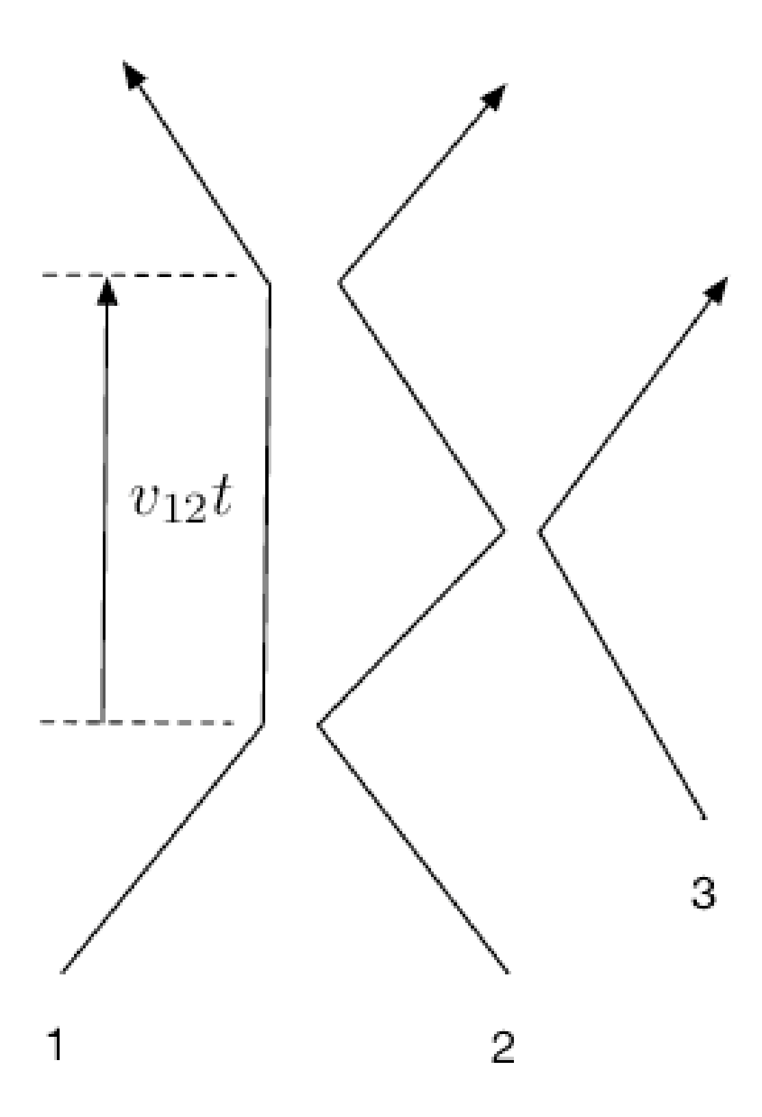
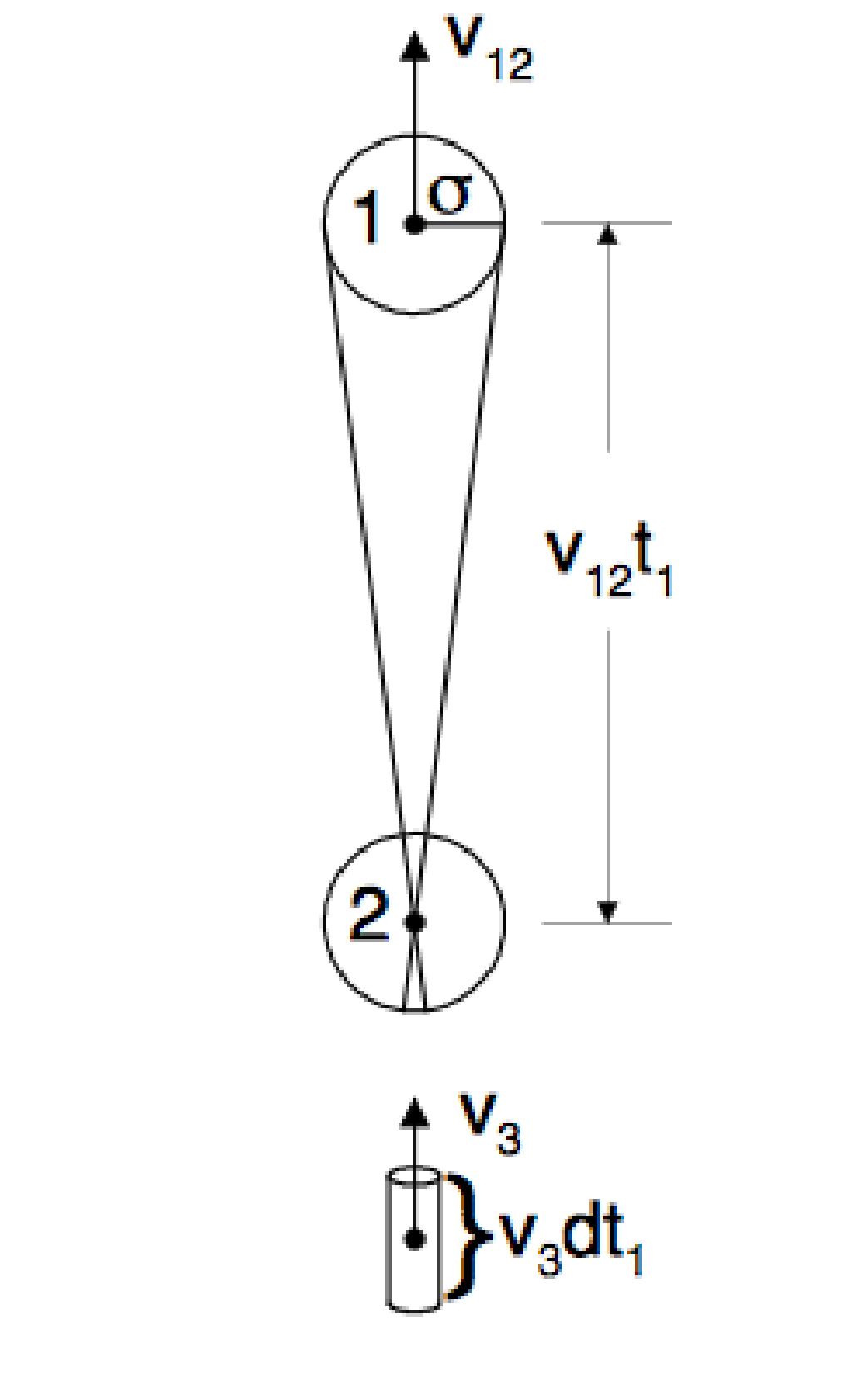
Figure 1: Three particle recollision event: Particles $1$and $2$ collide at some initial time, and due to an intermediate $(2,3)$ collision, particles $1$ and $2$ collide at a time $t$ later. The second figure is set in the rest frame of particle $2$, and shows the solid angle into which particle $2$ must be scattered by particle $3$ to collide with particle $1$ at time $t.$ Here $v_{12}$ is the relative velocity of particles $1$ and $2$ after the first collision.

The origin of these divergent coefficients can be easily understood by considering the coefficient $a{}_{1}^{(\xi)},$ for example. In Figure 1, we illustrate one of the three particle, correlated collision sequences that contribute to this coefficient[5, 11]. In this recollision event, particles $1$ and $2$ collide at some initial instant, then later, particle $3$ collides with particle $2$, in such a way that particles $1$ and $2$ collide again after a time interval $t$ between the first and last collisions between these two particles. The sequences take place in infinite space and over arbitrarily large times, $t$. As illustrated in the Figure, the dynamics is controlled by the solid angle into which particle $2$ must be scattered when particle $3$ hits it. The phase space region available for particle $3$ to cause the $(1,2)$ re-collision between time $t$ and $t+dt$ is proportional to the solid angle and is of the order $(\sigma/vt)^{d-1}dt$. The coefficient $a_{1}$ is determined by the integration of this region over all possible time intervals $t,$ and is clearly logarithmically divergent for $d=2.$ The coefficient $a_{1}^{(\xi)}$ is finite for $d=3,$ but the next coefficient, $a_{2}^{(\xi)},$ is logarithmically divergent for three-dimensional systems for similar reasons, and all higher coefficients diverge also, as powers of the upper limit on the time integral which can be arbitrarily large. Thus we can identify the essential difference between equilibrium and non-equilibrium properties of gases: non-equilibrium processes are due, among other things, to dynamical processes that can take place over large spatial distances and over large times. These processes cause long range and long time correlations among the particles in the gas that are absent in equilibrium, except perhaps at critical points, and even then, are of a qualitatively different origin. We are now faced with another problem. The results of Bogoliubov, Green, and Cohen are incomplete - their virial series are useless for descriptions of processes that take place over times long compared to some microscopic time due to the long time divergences in the terms in the virial series.

2 The Ring Resummation

It is clear what is causing the divergences in the non-equilibrium expansions. A collective effect, mean free path damping of trajectories has been ignored when deriving the virial expansions. We argued above that the virial coefficients depend on the dynamics of isolated groups of a fixed number of particles, and the time between any two collisions in the troublesome correlated collision sequences can be arbitrarily large. This is clearly unphysical. In a real gas, particles cannot travel arbitrarily long distances between collisions without another particle interrupting the motion of the particles by colliding with one of them. That is to say, the typical distance between collisions is a mean free path which in turn depends upon the gas density and temperature. The probability of a particle moving a certain distance is exponentially damped as the distance of travel becomes larger than a few mean free path lengths. In essence, by insisting that the collision operator or that the time correlation expressions be expanded in a power series in the gas density, one has taken what should be an exponential damping and expressed the exponential as a power series. Thus non-equilibrium virial expansions are very misleading since they are the equivalent of writing

$$e^{-nt} = 1-nt+\frac{1}{2}(nt)^{2}+\cdots,$$ (6)

and trying to determine the behavior of the exponential by examining individual terms on the right-hand side of its power series expansion. It is clear that a more physical representation of the generalized collision operator or of the time correlation function expressions should be obtained by summing the most divergent terms in the virial expansions and using the resummed expression, not the virial expansions. This resummation was first carried out by K. Kawasaki and I. Oppenheim in 1965[12]. They expressed the most divergent terms in the virial expansions as ring events and were able to resum these most divergent terms and to obtain expressions for transport coefficients that should be well behaved, in contrast to the virial expansion representations. For three-dimensional systems one can use the resummed expressions for transport coefficients to show that the logarithmic divergence in the virial expansion is replaced by a logarithmic term in the density, that results from including the mean free path damping in the relevant collision integrals. Thus the first few terms in the density expansion of the transport coefficients are

$$\frac{\xi(n,T)}{\xi_{0}(T)}=1+a_{1}^{(\xi)}n\sigma^{3}+a_{2,ln}^{(\xi)}(n\sigma^{3})^{2}\ln n\sigma^{3}+a_{2,n}^{(\xi)}(n\sigma^{3})^{2}+\cdots.$$ (7)

The coefficient of the linear term, $a_{1}^{(\xi)}$, had already been calculated by Sengers[13] for hard spheres, based on the analysis of this three-body collision integral by S. T. Choh and G. E. Uhlenbeck[14] and by Green[15]. Also for hard spheres the coefficient, $a_{2,ln}^{(\xi)},$ of the logarithmic term has been calculated[16], and estimates have been made of the coefficient $a_{2,n}^{(\xi)}$ using the Enskog theory. In Figure 2 we show the comparison of the theoretical and computer results for the coefficients of self-diffusion, shear viscosity, and thermal conductivity for a moderately dense gas of hard spheres[17]. The agreement is quite good despite the fact that the coefficient $a_{2,n}^{(\xi)}$ can only be estimated for reasons that will become clear below.

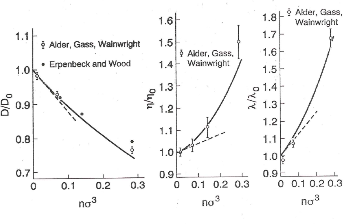
Figure 2: Comparison of the theoretical expressions, Eq. (7) for the transport coefficients of self-diffusion, $D,$ the coefficient of shear viscosity, $\eta$, and thermal conductivity, $\lambda,$ for a gas of hard spheres with the results of molecular dynamics[17, 18, 19]. The dashed lines correspond to keeping only the first two terms in this expansion. The coefficient $a_{2,n}^{(\xi)}$ is estimated using the Enskog theory.

The non-analytic terms in a density expansion of a transport coefficient have also been considered in quantum systems. Indeed, very early on J. S. Langer and T. Neal[20], motivated by the above classical work, pointed out that logarithmic terms appear in the electrical conductivity in disordered electronic systems. It can be argued that this sort of calculation, basically a quantum Lorentz gas, is also relevant for the electron mobility, $\mu$, of excess electrons in liquid helium. In this case the dimensionless density expansion parameter, $\chi=4na_{s}^{2}\lambda$, involves the thermal de Broglie wavelength, $\lambda=(2\pi^{2}\hbar^{2}/mk_{B}T)^{1/2}$, the density of helium atoms, $n$, and the $s-$wave scattering length $a_{s}$. Here $\hbar$ is Planck’s constant and $m$ is the electron mass. Wysokinski, Park, Belitz and Kirkpatrick[21, 22] have exactly computed $\mu$ up to and including terms of $O(\chi^{2})$ and obtained,

$$\mu/\mu_{B}=1+\mu_{1}\chi+\mu_{2ln}\chi^{2}ln\chi+\mu_{2}\chi^{2}+o(\chi^{2}).$$ (8)

Here $\mu_{B}$ is the Boltzmann equation value for $\mu$, and $\mu_{1}=-\pi^{3/2}/6,$ $\mu_{2ln}=(\pi^{2}-4)/32,$ and $\mu_{2}=0.236\ldots.$ Adams et al [23] have concluded that existing experiments give very good agreement with the value of the conductivity given by Eq. (8).

To test experimentally the presence or absence of the logarithmic term, Wysokinski et al defined the function,

$$f(\chi)=[\mu/\mu_{B}-1-\mu_{1}\chi]/\chi^{2}.$$ (9)

Theoretically,

$$f(\chi)=\mu_{2ln}ln\chi+\mu_{2}\pm 2\pi^{1/2}\chi,$$ (10)

where the last term is an estimate of the $O(\chi^{3})$ contribution to $\mu$. In Figure 3[21, 22] the theoretical prediction is shown for $0<\chi<0.7$ together with experimental data[24]. The error bars shown assume a total error of $3\%$ in $\mu/\mu_{B}$ and $4\%$ in $\chi$. To illustrate the effect of the logarithmic term, the figure also shows what the theoretical prediction would be if $\mu_{2ln}$ in Eq.(8) were zero.

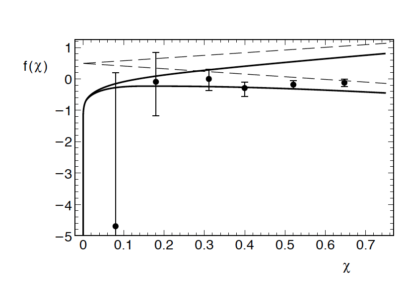
Figure 3: The reduced mobility f, as defined in Eq. (9), vs. the density parameter $\chi$. The theoretical prediction of Wysokinski, Park, Belitz, and Kirkpatrick is for f to lie between the two solid curves [21]. The experimental data are from Fig. 9 of Ref. [24] with error bars estimated as in the two possible forms of Eq. (10). The broken lines show what the theoretical prediction would be in the absence of the logarithmic term in the density expansion.

Following the discovery that logarithmic terms must appear in non-equilibrium density expansions, there were strong indications that something was still amiss in the kinetic theory for transport coefficients. In 1966 R. Goldman[25] argued that the resummed expressions for transport coefficients contain time integrals of functions with power-law decays. He identified the leading power as $t^{-3/2}$ for long times, for three-dimensional systems. In 1968 Y. Pomeau[26] argued that for two-dimensional systems the Kawasaki- Oppenheim expressions still diverge as time integrals of functions that decay as $t^{-1}$ for large times.

This was the situation just before the work of Alder and Wainwright on the velocity auto-correlation function became known, and before the appearance in 1970 of their paper in Physical Review which stimulated so much work in non-equilibrium statistical mechanics, and continues to reverberate even now with new and unexpected applications.

3 The Alder-Wainwright Paper of 1970: Long Time Tails

The papers by Alder and Wainwright in Physical Review Letters in 1967[27], and most especially, that in Physical Review in 1970[28] provided the spark that ignited the imaginations of those of us working in kinetic theory. They considered gases of hard spheres or of hard disks at moderate densities and by means of computer simulated molecular dynamics, obtained the velocity correlation function $\left\langle v_{x}(0)v_{x}(t)\right\rangle/\left\langle v_{x}^{2}\right\rangle$ for a range of times, scaled with the appropriate mean free time, $t_{m},$ between collisions. Their results provided convincing evidence that over a range of times, roughly $10\leq s=t/t_{m}\leq 30,$ the velocity autocorrelation functions decay as

$$\frac{\left\langle v_{x}(0)v_{x}(s)\right\rangle_{eq}}{\left\langle v_{x}^{2}\right\rangle_{eq}}\simeq\alpha_{D}^{(d)}(n)s^{-d/2}.$$ (11)

Here $\alpha_{D}^{(d)}(n)$ is a numerical coefficient that depends on the density and the spatial dimension of the gas. The subscript $D$ indicates that the time correlation function is the one needed for the coefficient of self- or tagged particle diffusion through Eq. (3). Figure 4 shows their results for the three-dimensional case.

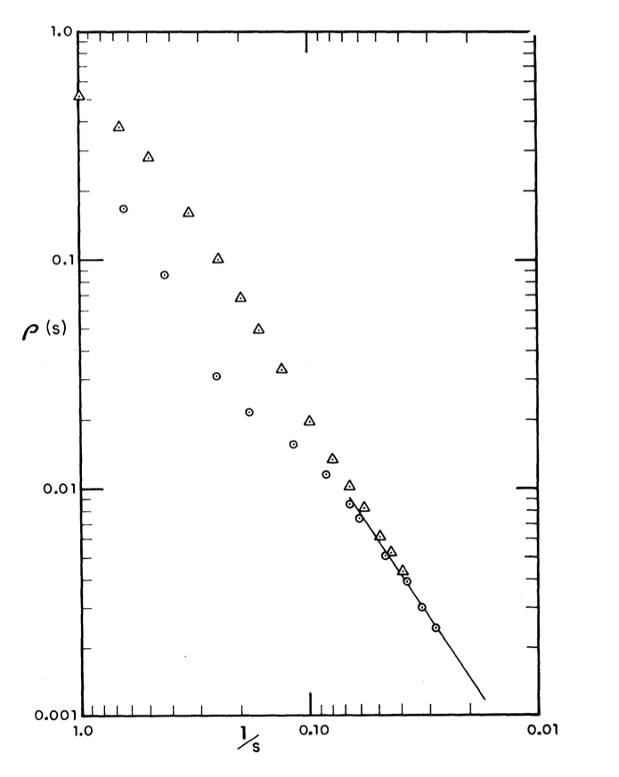
Figure 4: The normalized velocity autocorrelation function as obtained by molecular dynamics (triangles) for a gas of $500$ hard spheres[28]. The circles are results obtained using a hydrodynamical model developed by Alder and Wainwright to explain their results.

Stimulated by these computer results and following theoretical arguments of Goldman and Pomeau, Dorfman and Cohen[29, 30] were able to show that these algebraic decays can be explained both qualitatively and quantitatively by kinetic theory. They evaluated the Kawasaki-Oppenheim ring summation, but in order to obtain results appropriate for the densities studied by Alder and Wainwright, they extended the summation result to higher densities by means of the Enskog theory for dense hard ball gases[31]. At the same time Ernst, Hauge, and van Leeuwen[32] provided a mesoscopic argument for these algebraic decays , or as they are called now, long time tails. The expression for the coefficient $\alpha_{D}^{(d)}(n)$ will serve to illustrate a general feature of the theoretical explanation of the long time tails,

$$\alpha_{D}^{(d)}(n)=c_{d}\left[(D+\nu)t_{m}\right]^{-d/2}.$$ (12)

Here $c_{d}$ is a numerical coefficient and proportional to $n^{2-d}$, $D$ is the coefficient of self-diffusion, and $\nu=\eta/\rho$ is the kinematic viscosity, $\eta$ is the coefficient of shear viscosity and $\rho$ is the mass density of the fluid. The comparison of the kinetic theory results, using the Enskog theory for the transport coefficients with the results of Alder and Wainwright is illustrated in Figure 5 [29]. This provides conclusive proof that the Alder-Wainwright results can be explained by kinetic theory when the contributions of the most divergent terms are taken into account.

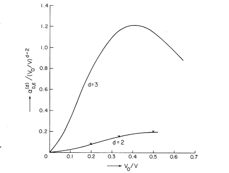
Figure 5: The solid curves are the theoretical results obtained by Dorfman and Cohen for the coefficients, $\alpha_{D,E}^{(d)}$ appearing in Eq. (12) for the velocity autocorrelation function, using Enskog theory values for the transport coefficients[29]. The crosses represent values obtained from molecular dynamics by Alder and Wainwright, for two-dimensional systems[28]. Here $V/V_{0}$ is the ratio of the volume of the system to that at close packing of the disks or spheres.

In Figure 6 we show later results of Wood and Erpenbeck[33] confirming those of Alder and Wainwright and they compared their results with theoretical results including finite size effects.

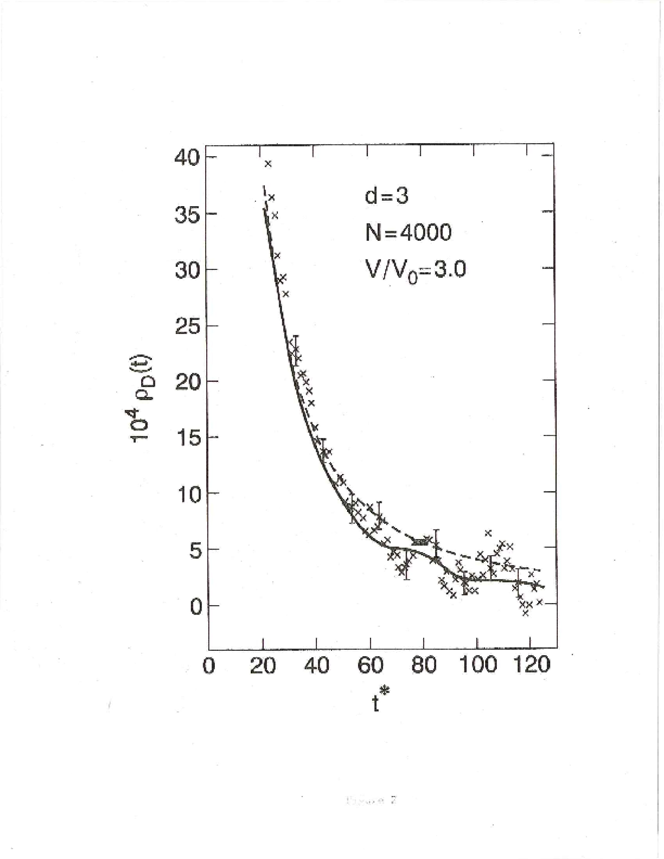
Figure 6: Results of Wood and Erpenbeck for the velocity autocorrelation function for a gas of $4000$ hard spheres at a volume of three times the close packing volume[34]. Here $t^{*}$ is the time, measures in mean free times. The crosses are computer results, the dashed line is that given by Eq. (11), and the solid line represents a complete evaluation of the mode coupling formula with all modes taken into account and finite size corrections included.

It is important to note that $\alpha_{D}^{(d)}$ depends upon the sum of two transport coefficients, in this case the coefficient of self-diffusion and the kinematic viscosity. This is an indication of the fact that the underlying microscopic processes generating the tails are the coupling of microscopic hydrodynamic modes that exist as fluctuations in fluids and are detected in dynamic light scattering experiments. The dynamical events taking place in the gas generate both the modes and their coupling. A simple example will illustrate the point. A somewhat oversimplified picture of a renormalized recollision illustrated in Fig. 1 is shown in Figure 7 [35]. Two particles collide at some instant of time, then undergo an arbitrary number of intermediate collisions before recolliding at time $t.$ One can think of the motions of the two particles after their first collision as random walks that cross at time $t.$ If we sit on one of the particles we can imagine that the recollision is a random walk that returns to the origin. A standard calculation in random walk theory shows that the probability of a return to the origin after a time interval $t$ is proportional to $(1/t)^{d/2}$. This time dependence is exactly that of the long time tails, and the random walks represent hydrodynamic processes such as diffusion that are coupled by the initial and final collisions.

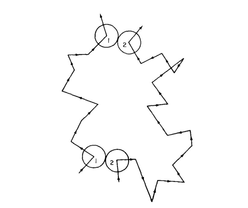
Figure 7: A schematic version of a renormalized recollision sequence. Two particles collide and then each of them undergoes a random walk produced by collisions with other particles before they collide again after a time $t.$

We thus have, when this is all worked out properly, a microscopic derivation of mode-coupling theory, already known from the work of L. P. Kadanoff and J. Swift[36] and of Kawasaki[37] on the behavior of transport coefficients near the critical point of a phase transition. In fact the Kadanoff-Swift results are exactly the combined result of the long time tail processes with the behavior of thermodynamic properties near a critical point. We also mention that the transport coefficients appearing in the expression for $\alpha_{D}^{(d)}$ have to be treated with some care. They cannot be the full transport coefficients since those are determined by the long time behavior of correlation functions. Instead, over the time of the Alder-Wainwright studies these are to be seen as short time contributions, thus accounting for the success of using the Enskog expressions for the transport coefficients when comparing the computer results with those from kinetic theory.

4 Consequences of the Long Time Tails for Hydrodynamics

The algebraic time decays of the time correlations and the existence of generic long range correlations in non-equilibrium systems have immediate consequences for microscopic derivations of the Navier Stokes and higher-order hydrodynamic equations. The most immediate of these is that the time correlation functions expressions for transport coefficients diverge logarithmically with the upper limit of the time integrals in the Green-Kubo formulas. For three-dimensional systems, the Navier Stokes transport coefficients are finite but transport coefficients in higher-order equations, such as the Burnett equations diverge[29, 32, 38, 39]. We are therefore faced with the fact that our microscopic derivations of the fluid dynamics equations have divergence problems. A number of studies have been carried out in order to determine a more correct form of these equations, free of divergence problems. The results are complicated and depend to a certain extent on the transport process. For example, for two-dimensional viscous flows, one finds that Newton’s law of viscous friction must be modified by the addition of non-linear logarithmic terms in the velocity gradients. For three-dimensional systems, there is a non-analytic correction to Newton’s law. That is the off-diagonal terms of the pressure tensor, $P_{xy},$ for example have the form[40, 41]

$$P_{xy}^{(2)} \simeq -\tilde{\eta}X+aX\ln X+\cdots,$$

$$P_{xy}^{(3)} \simeq -\eta X+bX|X|^{1/2}+\cdots,$$

$$X = \frac{\partial u_{x}(y)}{\partial y}.$$ (13)

Here $u_{x}(y)$ is the component of the fluid velocity, ${\bf u}$ that is a function of the coordinate in a perpendicular direction, as is appropriate for shear flow. We see that for two-dimensional systems, viscous flow is inherently nonlinear, since a coefficient of shear viscosity defined by the limit $\lim_{X\to 0}P_{xy}/X$ does not exist. For three-dimensional systems the corrections to Newton’s law are non-analytic; in this case, a fractional power of the velocity gradient appears. Physically, a finite shear rate weakens or makes shorter range the correlations that cause the divergence problems.

The same considerations have also been applied to the case of a stationary temperature gradient. Surprisingly, this case is very different. A finite $\nabla T$ does not fix the divergence problem in the two-dimensional heat conductivity, nor does it lead to non-analytic terms in the three-dimensional heat flux[42, 43]. This in turn implies that correlations in a non-equilibrium system with a temperature gradient are of longer range, and more robust, than a fluid with a velocity gradient. This observation is intimately tied to the striking results discussed in the next section.

For three-dimensional systems the dispersion relation for sound propagation in a gas also has a non-analytic form[44, 38],

$$\omega(k)=\pm ick+\frac{1}{2}\Gamma k^{2}+Ak^{5/2}+\cdots,$$ (14)

where $\omega(k)$ is the frequency of sound as a function of the wave number, $k,$ $c$ is the velocity of sound and $\Gamma$ is the sound damping constant. There are also an infinite number of terms between $k^{2}$ and $k^{3}$, only the first of which is given here. There is, indeed, some experimental evidence for the appearance of the $k^{5/2}$ term in this dispersion relation as seen from neutron scattering studies on liquid sodium[45]. It is possible to analyze the neutron scattering data in order to obtain values of the frequency dependence of the Fourier transform, $Z(\omega)$ of the velocity correlation function as a function of the frequency, $\omega$. The long time tail in this function would then be seen as a dependence of the Fourier transform on $\omega^{1/2}$. The results of Morkel et al are illustrated in Figure 8. The square root dependence is clear and the data are in good agreement with the theory.

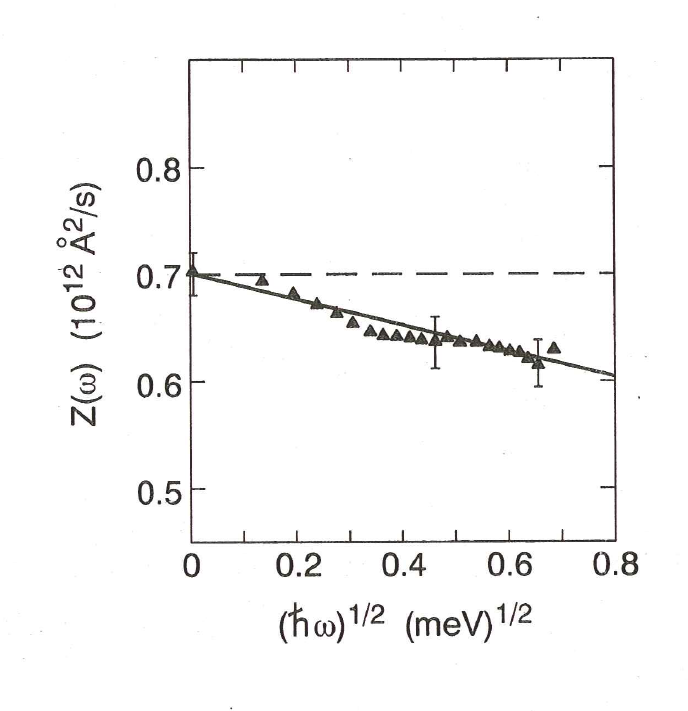
Figure 8: The Fourier transform of the velocity autocorrelation function, $Z(\omega)$ as a function of the square root of the frequency, $\omega,$ for atoms in liquid sodium as obtained from neutron scattering experiments (triangles). The solid line is the theoretical result including mode-coupling effects, while the dashed line omits them.[45]

In general, very little is known about the complete structure of the hydrodynamic equations, especially for two-dimensional systems. Non-analytic terms, finite size effects, branch point structures, and so on seem to be present. The only redeeming feature of all of this is that these complications do not appreciably distort the results obtained by using ordinary Navier Stokes hydrodynamics, even if, for two dimensions we can only give approximate results for the transport coefficients that appear in them.

5 Non-equilibrium Steady States

Very dramatic deviations from equilibrium behavior due to mode-coupling effects causing long range spatial correlations can be found in the properties of fluids maintained in non-equilibrium stationary states. The first striking example of this difference was discovered by Kirkpatrick[42], described in his doctoral dissertation and in a subsequent series of papers by Kirkpatrick, Cohen and Dorfman[46, 47, 48]. Confirmation of this work was obtained by Sengers and co-workers in a series of light scattering experiments on a fluid maintained in a steady state with a fixed temperature gradient. As we noted above the structure factor for an equilibrium fluid is, for small wave numbers, characterized by a central Rayleigh peak and two Brillouin peaks on either side of the central peak. All of this changes when a constant temperature gradient is imposed on the system. Most dramatic of these effects is the enhancement of the central peak by orders of magnitude, an enhancement due to the long range spatial correlations in a non-equilibrium fluid. When a temperature gradient is imposed on a fluid, the central peak of structure factor, $S_{neq}(t,{\bf k})$ for a simple fluid, is given for small wave numbers $k$ as a function of time, $t,$ by

$$S_{neq}(t,{\bf k}) = S_{0}\left[\left(1+A_{T}\right)e^{-D_{T}k^{2}t}-A_{\nu}e^{-\nu k^{2}t}\right],$$

$$A_{T} = \frac{c_{P}}{T\left(\nu^{2}-D_{T}^{2}\right)}\left(\frac{\nu}{D_{T}}\right)\frac{\left(\hat{{\bf k}}_{\perp}\cdot\nabla T\right)^{2}}{k^{4}},$$

$$A_{\nu} = \frac{c_{P}}{T\left(\nu^{2}-D_{T}^{2}\right)}\frac{\left(\hat{{\bf k}}_{\perp}\cdot\nabla T\right)^{2}}{k^{4}}.$$ (15)

Here $S_{0}$ measures the intensity of the thermal fluctuations when the fluid is in equilibrium, $c_{P}$ is the specific heat capacity at constant pressure, $\nu,D_{T}$ are the coefficients of kinematic viscosity and of thermal diffusivity, respectively, and $\hat{{\bf k}}_{\perp}$ is a unit vector in a direction perpendicular to that of the wave vector, ${\bf k}$. It is important to note the inverse fourth power of the wave number appearing in the coefficients $A_{T},A_{\nu}$, and the proportionality to the square of the component of the temperature gradient in a direction perpendicular to that of the wave vector. The strong dependence on the wave number indicates quite clearly that these effects are due to the long range nature of the spatial correlations in the fluid, and these terms vanish for zero temperature gradient. All the thermodynamic and transport coefficients are known for toluene, for example, so that a direct comparison of theory and experiment can be carried out, as was done by Sengers and co-workers[49]. The results are given in Figure 9. The agreement of theory and experiment is excellent.

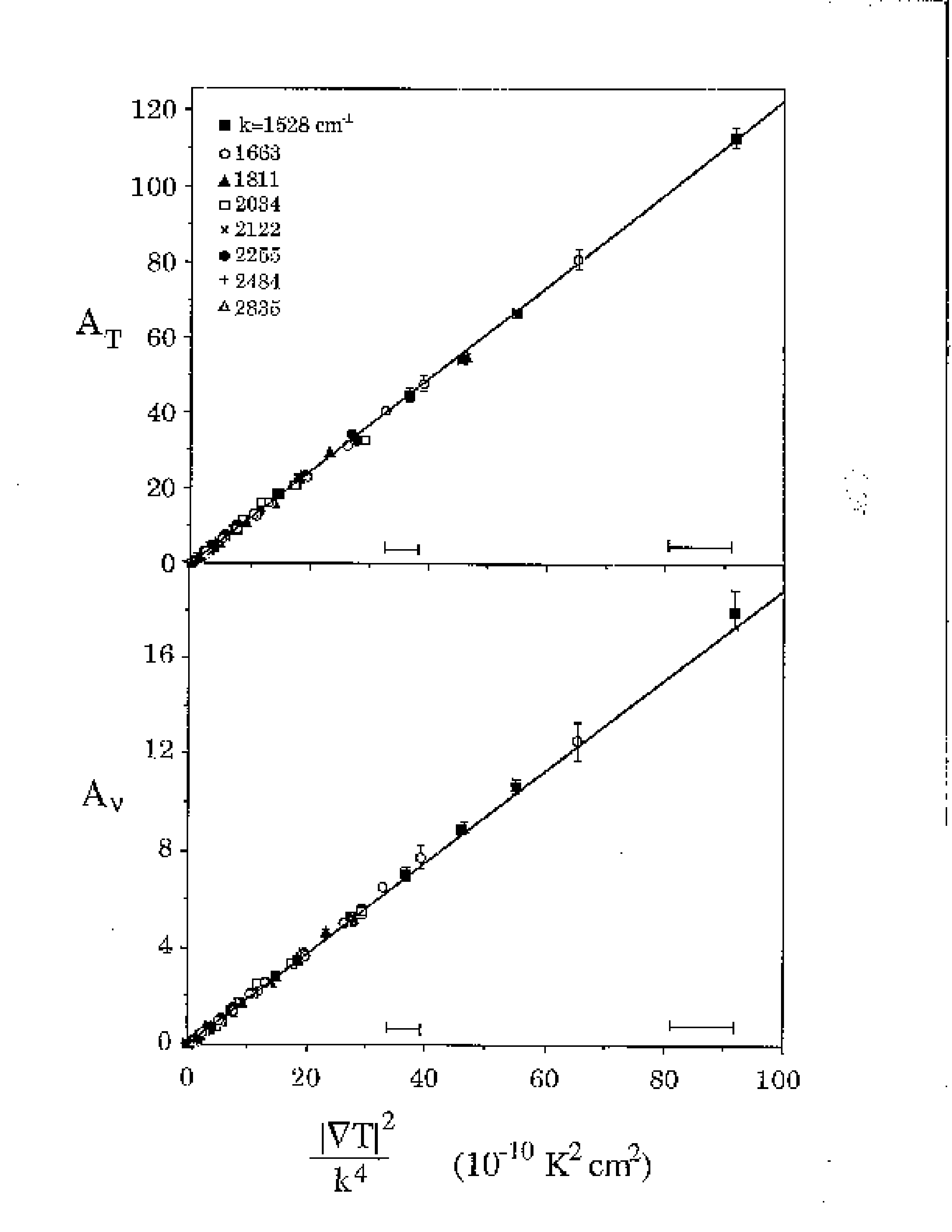
Figure 9: The coefficients $A_{T}$ and $A_{\nu}$ as a function of wave number as measured in light scattering experiments by Sengers et al [49]. The solid lines are theoretical values with no adjustable parameters.

Generally, long-ranged fluctuations will also induce a so-called Casimir force in a confined fluid[50]. A well known example is the Casimir effect due to critical fluctuations in equilibrium fluids[51, 52]. Critical fluctuations roughly vary as $k^{-2}$, while the above non-equilibrium fluctuations vary as $k^{-4}$. Hence, as shown by Kirkpatrick, Ortiz de Zárate, and Sengers[53, 54], Casimir effects in confined non-equilibrium fluids that are substantially larger than critical Casimir effects in equilibrium fluids. As an example, we consider a liquid between two horizontal thermally conducting plates separated by a distance $L$ and subject to a stationary temperature gradient $\nabla T$. The non-equilibrium Casimir effects are two fold. First, there will be a fluctuation-induced non-equilibrium contribution to the density profile as a function of height. Second, the fluctuations cause an additional non-equilibrium pressure contribution, $\bar{p}_{NE},$ to the equilibrium pressure such that[53, 54]

$$\overline{p}_{{\rm NE}}=\frac{c_{p}k_{{\rm B}}\overline{T_{0}}^{2}\left(\gamma-1\right)}{96\pi D_{T}\left(\nu+D_{T}\right)}\widetilde{B}F_{0}L\left(\frac{\nabla T_{0}}{\overline{T_{0}}}\right)^{2},$$ (16)

with,

$$\widetilde{B}=\left[1-\frac{1}{\alpha c_{p}}\left(\frac{\partial c_{p}}{\partial T}\right)_{p}+\frac{1}{\alpha^{2}}\left(\frac{\partial\alpha}{\partial T}\right)_{p}\right],$$ (17)

Here $\alpha$ is the thermal expansion coefficient, and $\gamma$ is the ratio of the isobaric and isochoric heat capacities. The coefficient $F_{0}$ is a numerical constant whose value depends on the boundary conditions for the velocity fluctuations that are coupled with the temperature fluctuations through the temperature gradient. For stress-free boundary conditions $F_{0}=1$. Just as in Eq. (15), all thermophysical properties, including the temperature $T$, can to a good approximation be identified with their average values in the liquid layer. Note that, for a given value of the temperature gradient $\nabla T$, the fluctuation-induced pressure increases with $L$. The physical reason is that the dependence of the fluctuations implies that in real space the correlations scale with the system size. This non-equilibrium pressure contribution corresponds to a nonlinear Onsager-like cross effect[53, 54]:

$$\bar{p}_{NE}=\kappa_{NL}(\nabla T)^{2},$$ (18)

where $\kappa_{NL}$ is a coefficient in the Burnett equations mentioned earlier in Section 4. Comparing Eqs. (16) and (18), we see that the non-equilibrium fluctuation-induced pressure is directly related to the divergence of the nonlinear Burnett coefficient $\kappa_{NL}$ with increasing $L$. Experimentally, it may be more convenient to investigate the fluctuation-induced pressure as a function of the temperature difference $\delta T=L\nabla T$. Then

$$\bar{p}_{NE}\propto\frac{1}{L}\left(\frac{\delta T}{T}\right)^{2}.$$ (19)

This result may be compared with the critical Casimir pressure in equilibrium fluids:

$$p_{c}=\frac{k_{B}T}{L^{3}}\Theta\left(\frac{L}{\xi}\right),$$ (20)

where $\xi$ is the correlation length. From Eq. (20), we have estimated that for water at $298$ K in a layer with $1$ micron and with $\delta T=25$ K , will be of the order of a Pa, while $p_{c}$ is of the order of a milli-Pa for the same distance. Actually, at $L=1$ mm, $\bar{p}_{NE}$ becomes already of the same order of magnitude as $p_{c}$ at $L=1$ micron. One should also note that the critical Casimir effect can only be observed in fluids near a critical point, while the non-equilibrium Casimir effect will be generically present in liquids at any temperature and density. We conclude that thermal fluctuations in non-equilibrium fluids are fundamentally different from thermal fluctuations in equilibrium fluids.

6 Long Time Tail Phenomena in Other Contexts

It is quite remarkable how often one encounters situations in other physical contexts where the long time tails or, equivalently, mode-coupling theory play an important role. Here we list just a few examples.

Critical Phenomena

As we mentioned earlier, mode-coupling theory was developed more or less intuitively by Kadanoff and Swift in order to explain the behavior of transport coefficients near the critical points of phase transitions, such as the liquid-gas transition. It was known from experiments of Sengers, carried out in the 1960’s, that the coefficient of thermal conductivity diverges near this critical point as recently reviewed by Anisimov[55]. In this situation both static and dynamic correlations have a long range. Later experiments of Sengers and co-workers confirmed both effects[56, 57]. The results were a combination of long time tail effects underlying mode-coupling theory with the effects of the singular behavior of thermodynamic properties of the fluid near its critical point. Other and related applications of mode-coupling theory to the liquid-glass transition have been important for the theory of glasses but we will not comment on that work here.

Weak Localization

In Section 2 we mentioned that in the mid $1960^{\prime}s$ Langer and Neal[20] showed that a logarithmic term appears in the conductivity in disordered electron systems. It wasn’t until the late $1970^{\prime}s$ that the dynamical consequences of the correlations that lead to the logarithmic term, basically quantum long-time tail effects, were studied and understood[58, 59]. This opened up the field of what became known as weak localization in condensed matter physics which in turn is closely connected to the phenomenon of Anderson localization[61]. Among other things, the ultimate conclusion was that the effects were so strong that at zero temperature a two-dimensional system is always an insulator[62, 59, 63, 64]. At finite temperature there are logarithmic temperature non-analyticities that decrease the conductivity as $T$ is lowered. In three dimensions there are weaker, but still important non-analyticities in both temperature and frequency. All of these effects have been measured in great detail. For reviews see Refs. [65, 66].

Cosmology

There appears to be a deep and interesting connection between long time tail phenomena that we have been discussing here and the results of investigations of the dynamics of black hole horizons. The cosmology community has become aware of the results of non-equilibrium statistical mechanics, in particular, the existence of long time tails and their anomalous effects on the equations of fluid dynamics. We will not go into the details but it is worth mention the titles of a few recent papers: “Hydrodynamic Long Time Tails from Anti de Sitter Space” by S. Caron-Huot and O. Saremi[67], and “Hydrodynamic Fluctuations, Long Time Tails, and Supersymmetry” by P. Kovtun and L. G. Yaffe[68], among others. Such connections reinforce the notion gained from experience that across a wide swath of physics, people, perhaps without being aware of it, are working on the same or closely related problems, and the only difference is in the mathematical language used to describe them.

7 Conclusion

The paper has given a brief review of the history of kinetic theory and related non-equilibrium statistical mechanics with an emphasis of the work of Alder and Wainwright as described in their 1970 paper. Alder and Wainwright helped consolidate prior work in kinetic theory and stimulated much more work in theoretical, experimental, and computational physics. We hope that we have made clear the profound influence the 1970 paper has had on non-equilibrium statistical mechanics and on fields that on first sight might seem to be distantly related but on closer inspection turn out to be closely related after all. We are pleased to dedicate this paper to our friend, colleague and mentor, Berni Alder, on the occasion of his 90th birthday!

8 Acknowledgement

The authors would like to thank D. Belitz and D. Thirumalai for helpful discussions and Y. Bar Lev and A. Nava-Tudela for their considerable help with the preparation of this paper. They would also like to thank E. G. D. Cohen for useful and productive conversations over a period of many years. TRK would like to thank the NSF for support under Grant No. DMR-1401449

References

- [1] N. N. Bogoliubov. In J. de Boer and G. E. Uhlenbeck, editors, Studies in Statistical Mechanics, volume 1, pages 1–118. North-Holland, Amsterdam, 1961.
- [2] M. S. Green. J. Chem. Phys., 25:836, 1956.
- [3] E. G. D. Cohen. Physica, 28:1025, 1962.
- [4] E. G. D. Cohen. J. Math. Phys., 4:183, 1963.
- [5] M. S. Green and R. A. Piccirelli. Phys. Rev., 132:1388, 1963.
- [6] M. S. Green. J. Chem. Phys., 20:1281, 1952.
- [7] M. S. Green. J. Chem. Phys., 22:398, 1954.
- [8] R. Kubo. J. Phys. Soc. Japan, 12:370, 1957.
- [9] J. R. Dorfman and E. G. D. Cohen. Phys. Lett., 16:124, 1965.
- [10] S. G. Brush. Kinetic Theory, volume 3. Pergamon, New York, 1972.
- [11] J. R. Dorfman and E. G. D. Cohen. J. Math. Phys., 8:282, 1967.
- [12] K. Kawasaki and I. Oppenheim. Phys. Rev., 139:1763, 1965.
- [13] J. V. Sengers. In W. E. Brittin, editor, Boulder Lectures in Theoretical Physics, volume IX C, pages 335–374. Gordon and Breach, 1967.
- [14] S. T. Choh and G. E. Uhlenbeck. The kinetic theory of dense gases. Technical report, University of Michigan, 1958.
- [15] M. S. Green. Phys. Rev., 136:905, 1964.
- [16] B. Kamgar-Parsi and J. V. Sengers. Phys. Rev. Lett., 51:2163, 1983.
- [17] J. R. Dorfman, T. R. Kirkpatrick, and J. V. Sengers. In Ann. Rev. Phys. Chem., volume 45, page 213. Annual Reviews, 1994.
- [18] B. J. Alder, D.M. Gass, and T. E. Wainwright. J. Chem. Phys., 53:3813, 1970.
- [19] J. J. Erpenbeck and W. W. Wood. Phys. Rev. A, 43:4254, 1991.
- [20] J. S. Langer and T. Neal. Phys. Rev. Lett., 16:984, 1966.
- [21] K. I. Wysokinski, W. Park, D. Belitz, and T. R. Kirkpatrick. Phys. Rev. Lett., 73:2571, 1994.
- [22] K. I. Wysokinski, W. Park, D. Belitz, and T. R. Kirkpatrick. Phys. Rev. E, 52:612, 1995.
- [23] P. W. Adams, D. Browne, and M. A. Paalanen. Phys. Rev. B, 45:8837, 1992.
- [24] K. Schwartz. Phys. Rev. B, 21:5125, 1980.
- [25] R. Goldman. Phys. Rev. Lett., 17:130, 1966.
- [26] Y. Pomeau. Phys. Rev. A, 3:1174, 1971.
- [27] B. J. Alder and T. E. Wainwright. Phys. Rev. Lett., 18:988, 1967.
- [28] B. J. Alder and T. E. Wainwright. Phys. Rev. A, 1:18, 1970.
- [29] J. R. Dorfman and E. G. D. Cohen. Phys. Rev. Lett., 25:1257, 1970.
- [30] J. R. Dorfman and E. G. D. Cohen. Phys. Rev. A, 6:776, 1972.
- [31] J. R. Dorfman and E. G. D. Cohen. Phys. Rev. A, 12:292, 1975.
- [32] M. H. Ernst, E. H. Hauge, and J. M. J. van Leeuwen. Phys. Rev. Lett., 25:1254, 1970.
- [33] W. W. Wood and J. J. Erpenbeck. In Ann. Rev. Phys. Chem., volume 27, page 319. Annual Reviews, 1976.
- [34] W. W. Wood and J. J. Erpenbeck. Ann. Rev. Phys. Chem., 27:319, 1976.
- [35] J. R. Dorfman. Physica A, 106:77, 1981.
- [36] L. P. Kadanoff and J. Swift. Phys. Rev., 166:89, 1966.
- [37] K. Kawasaki. Ann. Phys., 61:1, 1970.
- [38] M. H. Ernst and J. R. Dorfman. J. Stat. Phys., 12:311, 1975.
- [39] Y. Pomeau and P. Resibois. Phys. Rept., 19:63, 1975.
- [40] M. H. Ernst, B. Cichocki, J. R. Dorfman, J. Sharma, and H. van Beijeren. J. Stat. Phys., 18:237, 1978.
- [41] A. Onuki. Phys. Lett. A, 70:31, 1979.
- [42] T. R. Kirkpatrick. PhD thesis, Rockefeller University, New York, 1981.
- [43] T. R. Kirkpatrick and J. R. Dorfman. Phys. Rev. E, 92:022109, 2015.
- [44] Y. Pomeau. Phys. Rev. A, 7:1134, 1973.
- [45] C. Morkel and C. Gronemeyer. Z. Phys. B, 72:433, 1988.
- [46] T. R. Kirkpatrick, E. G. D. Cohen, and J. R. Dorfman. Phys. Rev. A, 26:950, 1982.
- [47] T. R. Kirkpatrick, E. G. D. Cohen, and J. R. Dorfman. Phys. Rev. A, 26:972, 1982.
- [48] T. R. Kirkpatrick, E. G. D. Cohen, and J. R. Dorfman. Phys. Rev. A, 26:995, 1982.
- [49] P. N. Segré, R. W. Gammon, J. V. Sengers, and B. Law. Phys. Rev. A, 45:714, 1992.
- [50] M. Kardar and R. Golestanian. Rev. Mod. Phys., 71:1233, 1999.
- [51] M. E. Fisher and P. de Gennes. C. R. Acad. Sci. Paris B, 287:207, 1978.
- [52] M. Krech. The Casimir Effect in Critical Systems. World Scientific, Singapore, 1994.
- [53] T. R. Kirkpatrick, J. M. Ortiz de Zárate, and J. V. Sengers. Phys. Rev. Lett., 110:235902, 2013.
- [54] T. R. Kirkpatrick, J. M. Ortiz de Zárate, and J. V. Sengers. Phys. Rev. E, 89:022145, 2014.
- [55] M. A. Anisimov. Int. J. Thermophys., 32:2001, 2011.
- [56] R. F. Chang, H. Burstyn, J. V. Sengers, and A. J. Bray. Phys. Rev. Lett., 37:1481, 1976.
- [57] H. C. Burstyn and R. F. Chang. Phys. Rev. Lett., 44:410, 1980.
- [58] L. P. Gorkov, A. Larkin, and D. E. Khmelnitskii. JETP Lett., 30(228), 1979.
- [59] E. Abrahams, P. W. Anderson, D. C. Licciardello, and T. V. Ramakrishnan. Phys. Rev. Lett, 42:673, 1979.
- [60] D. Belitz, T. R. Kirkpatrick, and T. Vojta. Rev. Mod. Phys., 77:579, 2005.
- [61] P. W. Anderson. Phys. Rev., (1492), 1958.
- [62] F. Wegner. Z. Phys. B, 35:207, 1979.
- [63] L. Schafer and F. Wegner. Z. Phys. B, 231:113, 1980.
- [64] F. Wegner. Z. Phys. B, 36:209, 1980.
- [65] P. A. Lee and T. V. Ramakrishnan. Rev. Mod. Phys., 57:287, 1985.
- [66] D. Belitz and T. R. Kirkpatrick. Rev. Mod. Phys., 66:261, 1994.
- [67] S. Caron-Huot and O. Saremi. J. High Ener. Phys., 13:1, 2010.
- [68] P. Kovtun and L. G. Yaffe. Phys. Rev. D, 68:025007, 2003.