On bimodal size distribution of spin clusters in the one dimensional Ising model

Abstract

The size distribution of geometrical spin clusters is exactly found for the one dimensional Ising model of finite extent. For the values of lattice constant $\beta$ above some “critical value” $\beta_{c}$ the found size distribution demonstrates the non-monotonic behavior with the peak corresponding to the size of largest available cluster. In other words, at high values of lattice constant there are two ways to fill the lattice: either to form a single largest cluster or to create many clusters of small sizes. This feature closely resembles the well-know bimodal size distribution of clusters which is usually interpreted as a robust signal of the first order liquid-gas phase transition in finite systems. It is remarkable that the bimodal size distribution of spin clusters appears in the one dimensional Ising model of finite size, i.e. in the model which in thermodynamic limit has no phase transition at all.

Keywords: Phase transitions, small systems, bimodal distribution

I Introduction

During last two decades the experimental studies of phase transitions in finite and even in small systems are inspiring the high interest to their rigorous theoretical treatment Gross ; ComplMoretto ; Bmodal:Chomaz01 ; CSMM . One of the main reasons for such an interest is that the nuclear systems which are experimentally studied at intermediate JoeNat ; Pichon ; Bonnet and at high Pratt ; Karsch13 collision energies have no thermodynamic limit due to the presence of the long range Coulomb interaction and, hence, in a strict thermodynamical sense the phase transition in such systems is not defined. Therefore, the practical need to formulate the reliable experimental signals of phase transformations in the systems consisting of a few hundreds or thousands particles lead researchers to development of the non-traditional statistical methods which may be suited to small systems Bmodal:Chomaz01 ; CSMM ; Chomaz03 ; Bugaev05 ; Bmodal:Bugaev13 . One of such directions of research, the concept of bimodality, is based on the old T. L. Hill idea THill:1 that in finite system the interface between two pure phases “costs” additional free energy and, hence, their coexistence is suppressed. The practical conclusion coming out of this idea is that the resulting distribution of the order parameter should demonstrate a bimodal behavior and, hence, each maximum or peak of the bimodal distribution has to be associated with the pure phase THill:1 ; Bmodal:Chomaz01 ; Chomaz03 ; Bmodal:Chomaz03 ; Bmodal:Gulm04 ; Bmodal:Gulm07 .

Although in Bmodal:Chomaz03 the authors claimed to establish the one-to-one correspondence between the bimodal structure of specially constructed partition of some measurable quantity, known on average, and the properties of the Lee-Yang zeros YangLee of this partition in the complex plane of fugacity of this measurable quantity, there appeared certain doubts CSMM ; Lopez ; Bmodal:Bugaev13 about so strict relation between the bimodal-like mass/charge distributions of nuclear fragments and the liquid-gas nuclear phase transition in finite systems. In particular, the doubts follow from the experimental analysis of high momentum decay channels in nucleus-nucleus collisions Lopez and from the exact analytical solutions of the simplified statistical multifragmentation model Mekjian found for finite Bugaev05 ; Bmodal:Bugaev13 ; CSMM and infinite Sagun14 volumes. Two explicit counterexamples suggest that the bimodal mass distribution of nuclear fragments appears in a finite volume analog of gaseous phase Bmodal:Bugaev13 with positive surface tension and that it can also occur in the thermodynamic limit at supercritical temperatures Sagun14 , if at such temperatures there exists negative surface tension.

Despite the existing counterexamples Bmodal:Bugaev13 ; Sagun14 , up to now it is unclear, whether the statistical systems without phase transition can, in principle, generate the bimodal size distributions of their constituents for finite volumes. In order to demonstrate that this is, indeed, the case and the statistical systems in finite volume can generate the bimodal size distributions, here we analytically calculate the size distribution of geometrical spin clusters of the simplest statistical model which has no phase transition, the one dimensional Ising model Ising . Another principal purpose of this work is to further develop connections between the spin models and cluster models.

The cluster models are successfully applied to study phase transitions in simple liquids Fisher ; Dillmann ; Ford , in nuclear matter Bondorf ; CSMM ; Sagun14 ; Mekjian ; Bmodal:Bugaev13 ; Bugaev05 and in the quark-gluon plasma phenomenology Kapusta ; Gorenstein ; QGBSTM ; QGBSTM2 ; QGBSTM3 ; CGreiner:06 ; CGreiner:07 ; Koch:09 . Their basic assumption is that the properties of studied system consisting from the elementary degrees of freedom (molecules, nucleons, partons, etc.) can be successfully described in terms of physical clusters (vapor droplets, nucleus, hadrons, etc.) formed by any natural number of the elementary degrees of freedom. Since the cluster models proved to be a successful tool to investigate the phase transition mechanisms both in finite and in infinite systems, it seems that the development of equivalent cluster formulation for the well-known spin models and the determination of the properties of their physical clusters is a theoretical task of high priority. It is necessary to mention that some results on such a connection were already reported in ComplMoretto , in which a parameterization of the Fisher liquid droplet model Fisher was successfully applied to the numerical description of cluster multiplicities of two- and three-dimensional Ising model. However, below we implement this program to the one dimensional Ising model and directly calculate the size distribution of the geometrical spin clusters from the corresponding partition function.

The work is organized as follows. In the next section we explain the necessary mathematical aspects of calculating the spin cluster size distribution. Then, in Sect. 3 the derived expression is analyzed in details and the physical origin of bimodality in the present model is discussed. The results of our numerical simulations are also presented in this section. Finally, our conclusions and perspectives of further research are summarized in Sect. 4.

II Cluster size distribution

Here we use the geometrical definition of clusters which seems to be the most natural for lattice models. Within this framework the monomers, the dimers, the trimers and so on are built from the neighboring spins of the same direction. This approach is useful for different lattice systems ComplMoretto ; Moretto ; Fortunato2000 ; Fortunato2001 . A high level of its generality allows one to study the SU(2) and SU(3) gauge lattice models in terms of the clusters composed from the Polyakov loops Gattringer2010 ; Gattringer2011 ; Regensburg15 ; Kiev15 . Let’s consider the one dimensional Ising model in which spins are arranged in a linear lattice of size $N$ and they can be in two states only (up or down). Interaction energy of two neighboring spins is proportional to their product. Hence, the neighboring pair of parallel spins contribute $-\epsilon$ to the total energy of the system, whereas the corresponding contribution of the neighboring pair of antiparallel spins is $\epsilon$. For a convenience we choose the following boundary conditions: two edge spins have only a single neighbor which is able to interact with them.

Evidently, in the present model there are only two types of clusters, i.e. the clusters composed of spins up and of spins down. Hence, for a convenience hereafter they are called the up clusters and the down clusters and are marked with the superscripts $\uparrow$ and $\downarrow$, respectively.

The cluster multiplicities are defined as their occupancy numbers $n^{\uparrow}_{k}$ and $n^{\downarrow}_{k}$, where $k$ is the cluster size. It is clear that size of the maximal cluster can not exceed $N$ and, hence, only the spin configurations obeying the condition $n^{\uparrow}_{k>N}=n^{\downarrow}_{k>N}=0$ can be realized in the considered system. The total numbers of up and down spin clusters are, respectively, denoted as $n^{\uparrow}\equiv\sum_{k}n^{\uparrow}_{k}$ and $n^{\downarrow}\equiv\sum_{k}n^{\downarrow}_{k}$. Hereafter, it is assumed that the blind index of cluster size runs over all positive integers. In what follows the set of all occupancy numbers $\sigma\equiv\{n^{\uparrow}_{k},n^{\downarrow}_{k}\}$ is called as a microscopic configuration. Each microscopic configuration $\sigma$ of the system defines its total energy, which receives a contribution $\epsilon(1-k)$ from every up cluster or from every down cluster of size $k$. In addition, there exist the contacts of neighboring clusters with opposite spins and their number is $n^{\uparrow}+n^{\downarrow}-1$. Evidently, any such a contact gives a contribution $\epsilon$ to the system energy. Therefore, using the definitions of $n^{\uparrow}$ and $n^{\downarrow}$ we can cast the total energy of the system for a given microscopic configuration $\sigma$ as

$$H_{\sigma}=\epsilon\left[\sum_{k=1}^{\infty}(2-k)n^{\uparrow}_{k}+\sum_{k=1}^{\infty}(2-k)n^{\downarrow}_{k}-1\right].$$ (1)

Obviously, the total number of spins $N_{\sigma}\equiv\sum_{k}(n^{\uparrow}_{k}+n^{\downarrow}_{k})k$ should coincide with the lattice size $N$. Since up and down clusters alternate each other, then the only configurations with $n^{\uparrow}-n^{\downarrow}=0,~{}\pm 1$ can be realized in the considered system. Hence, taking into account the fact that the total number of cluster permutations is $n^{\uparrow}!n^{\downarrow}!/\prod_{k}n^{\uparrow}_{k}!n^{\downarrow}_{k}!$ we write the degeneracy factor of the microscopic configuration $\sigma$ as

$$G_{\sigma}=\frac{\delta_{N,N_{\sigma}}(2\delta_{n^{\downarrow},n^{\uparrow}}+\delta_{n^{\downarrow}+1,n^{\uparrow}}+\delta_{n^{\downarrow},1+n^{\uparrow}})n^{\uparrow}!n^{\downarrow}!}{\prod\limits_{k=1}^{\infty}n^{\uparrow}_{k}!n^{\downarrow}_{k}!},$$ (2)

where $\delta$ is the Kronecker delta-symbol. Note that every configurations with $n^{\downarrow}=n^{\uparrow}$ should have a degeneracy 2, since it can be “constructed” only from the configurations $n^{\downarrow}+1=n^{\uparrow}$ and $n^{\downarrow}=1+n^{\uparrow}$ by combining one of their outer clusters with any other cluster of the spin sign which coincides with the one of outer cluster.

The $q^{th}$ statistical moment of the down cluster occupancy number we define as

$$\langle{n^{\downarrow}_{l}}^{q}\rangle=\frac{1}{Z}\sum_{\sigma}\left[n^{\downarrow}_{l}\right]^{q}G_{\sigma}\,e^{-\frac{H_{\sigma}}{T}+a\beta(N_{\sigma}-N)},$$ (3)

where $T$ is the temperature and $\beta=\epsilon/T$ is the lattice constant. A summation over the configurations $\sigma$ in (3) should be understood as a summation over all nonnegative integers $n_{k}^{\uparrow}$ and $n_{k}^{\downarrow}$. The dimensionless parameter $a$ is introduced into (3) for the convenience of analytical calculations and its value is chosen to satisfy the conditions $\beta(a+1)<0$ and $\beta a<-\ln\left(2\cosh\beta\right)$. However, this parameter does not affect any observable due to the condition $N_{\sigma}=N$ provided by the Kronecker delta-symbols in Eq. (2).

Note, that $q=0$ yields the partition function $Z$, whereas a symmetry between up and down spins leads to the equality $\langle{n^{\uparrow}_{l}}^{q}\rangle=\langle{n^{\downarrow}_{l}}^{q}\rangle$. Using Eqs. (1) and (2), the definition of $N_{\sigma}$ along with the integral representation of the Kronecker delta-symbol $\delta_{r,s}=\int_{0}^{2\pi}\frac{d\alpha}{2\pi}e^{i\alpha(r-s)}$ and of the factorials $n^{\uparrow\downarrow}!=\int_{0}^{\infty}dz~{}e^{-z}z^{n^{\uparrow\downarrow}}$ we can write

$$\langle{n^{\downarrow}_{l}}^{q}\rangle = \frac{e^{\beta(1-aN)}}{Z}\int\limits_{0}^{2\pi}\frac{d\psi}{2\pi}e^{i\psi N}\int\limits_{0}^{2\pi}\frac{d\phi}{2\pi}(2+e^{i\phi}+e^{-i\phi})\int\limits_{0}^{\infty}dx~{}e^{-x}\int\limits_{0}^{\infty}dy~{}e^{-y}$$ (4)

$$\prod_{k=1}^{\infty}\sum_{n_{k}^{\uparrow}=0}^{\infty}\frac{\left(xe^{\beta(k(a+1)-2)-i\phi-i\psi k}\right)^{n^{\uparrow}_{k}}}{n^{\uparrow}_{k}!}\prod_{k=1}^{\infty}\sum_{n_{k}^{\downarrow}=0}^{\infty}\frac{\left(ye^{\beta(k(a+1)-2)+i\phi-i\psi k}\right)^{n^{\downarrow}_{k}}}{n^{\downarrow}_{k}!}~{}{n^{\downarrow}_{l}}^{q}.~{}$$

Now the summations over $n^{\uparrow}_{k}$ and $n^{\downarrow}_{k\neq l}$ in (4) can be performed trivially giving the corresponding exponential functions. In what follows we are mainly interested in finding the statistical moments of $n^{\downarrow}_{l}$ of the zeroth and first order. For $q=\{0;1\}$ the summation over $n^{\downarrow}_{l}$ generates an exponential function multiplied by the factor $(ye^{\beta(l(a+1)-2)+i\phi-i\psi l})^{q}$. Then, each product over $k$ in (4) can be carried out, since it is equivalent to a summation of decreasing geometric progressions in the exponential. In addition, the chosen range of $a$ provides a convergence of the integrals over $x$ and $y$ variables due to negative real part of these exponential functions. Hence, for $q=0$ and $1$ one can easily find

$$\langle{n^{\downarrow}_{l}}^{q}\rangle=\frac{e^{\beta(q(l-2)+1)}}{Z}\oint\limits_{|\zeta|=e^{-a\beta}}\frac{d\zeta~{}\zeta^{N-ql-1}}{2\pi i}\oint\limits_{|\xi|=1}\frac{d\xi~{}(2+\xi+\xi^{-1})\xi^{q}}{2\pi i\left(\xi-\frac{e^{-\beta}}{\zeta-e^{\beta}}\right)\left(1-\frac{\xi e^{-\beta}}{\zeta-e^{\beta}}\right)^{q+1}},$$ (5)

where the real variables of integration $\phi$ and $\psi$ are now changed to the complex ones $\xi=e^{i\phi}$ and $\zeta=e^{i\psi-a\beta}$. The integrand with respect to the variable $\xi$ in Eq. (5) contains three poles. The first one $\xi=0$ exists for $q=0$ only. However, the contribution of this pole does not produce any singularity with respect to the $\zeta$ variable and, hence, it can be safely neglected. The second pole existing at any value of $q$ corresponds to $\xi=\frac{\zeta-e^{\beta}}{e^{-\beta}}$. It does not contribute to $\langle{n^{\downarrow}_{l}}^{q}\rangle$ since it is located out of the contour $|\xi|=1$ due to the chosen value of the regularization parameter $a$. Thus, accounting only for the simple pole $\xi=\frac{e^{-\beta}}{\zeta-e^{\beta}}$ we obtain

$$\langle{n^{\downarrow}_{l}}^{q}\rangle=\frac{e^{\beta(q(l-3)+2)}}{Z}\oint\limits_{|\zeta|=e^{-a\beta}}\frac{d\zeta}{2\pi i}\frac{\zeta^{N-ql-1}(\zeta-2\sinh\beta)^{1-q}(\zeta-e^{\beta})^{q+1}}{(\zeta-2\cosh\beta)^{q+1}}.$$ (6)

This expression clearly demonstrates that for $q=1$ and $l=N$ the integral function has a specific simple pole $\zeta=0$ which, as we discuss below, is responsible for the non-monotonic behavior of $\langle n^{\downarrow}_{l}\rangle$.

Taking $q=0$ we immediately reproduce the well-known partition function of the one dimensional Ising model with free edges Ising , i.e.

$$Z=e^{2\beta}\oint\limits_{|\zeta|=e^{-a\beta}}\frac{d\zeta~{}\zeta^{N-1}(\zeta-2\sinh\beta)(\zeta-e^{\beta})}{2\pi i(\zeta-2\cosh\beta)}=2(2\cosh\beta)^{N-1}.$$ (7)

For $l\leq N$ the average occupancy number of the down clusters is obtained from Eq. (6) for $q=1$

$$\langle n^{\downarrow}_{l\leq N}\rangle = \frac{e^{\beta(1-l)}}{Z}\oint\limits_{|\zeta|=e^{-a\beta}}\frac{d\zeta~{}\zeta^{N-l-1}(\zeta-e^{\beta})^{2}}{2\pi i(\zeta-2\cosh\beta)^{2}}=\frac{\delta_{N,l}+2e^{-2\beta}+(N-l+1)e^{-4\beta}}{2(1+e^{-2\beta})^{l+1}},$$ (8)

whereas $\langle n^{\downarrow}_{l>N}\rangle=0$. Note, that $\langle n^{\uparrow}_{l}\rangle=\langle n^{\downarrow}_{l}\rangle$ for all $l$. The direct calculation based on this expression demonstrates that $\sum_{l}l\langle n^{\uparrow}_{l}\rangle=\sum_{l}l\langle n^{\downarrow}_{l}\rangle=N/2$ which is an obvious consequence of the symmetry between the spins up and down, if the external magnetic field is absent.

An explicit expression (8) for $\langle n^{\downarrow}_{l}\rangle$ allows us to find the size distribution function of clusters $\omega_{l}$ which is proportional to their average occupancy number. Since the size distribution functions are the same for both kinds of clusters, we do distinguish them. The normalized distribution $\omega_{l}$ is obtained from the condition that the total probability to find up (or down) cluster of any size is $1/2$, i. e. $\sum_{l}\omega_{l}=1/2$. This condition follows from the symmetry between up and down spins. Hence, we obtain

$$\omega_{l\leq N}=\frac{\delta_{N,l}+2e^{-2\beta}+(N-l+1)e^{-4\beta}}{2(1+Ne^{-2\beta})(1+e^{-2\beta})^{l}}\,,$$ (9)

and $\omega_{l>N}=0$. From Eq. (9) one can see that $\omega_{l}$ has not only the exponential part $(1+e^{-2\beta})^{-l}$, but also it includes the factor which is linear in $l$. The power part of the size distribution functions is known in several statistical models of cluster type. Traditionally it is taken into account by the Fisher topological exponent $\tau$ as $l^{-\tau}$ Fisher ; Bondorf ; CSMM ; QGBSTM . However, the linear $l$-part of the size distribution function (9) disappears in the thermodynamic limit $N\rightarrow\infty$, since in this limit one finds $\omega_{l}\rightarrow e^{-2\beta}(1+e^{-2\beta})^{-l}/2$. Hence, it is interesting to analyze the distribution $\omega_{l}$ of other lattice models in order to find possible restrictions on values of the Fisher index $\tau$.

III Bimodality manifestation

The growing interest to a bimodality is caused by the widespread belief that it can serve as a robust signal of the first order phase transition in finite systems. As it was mention above this concept is based on T. L. Hill idea THill:1 that, each peak of the bimodal distribution is associated with a pure phase. However, this idea cannot be sufficiently justified, since in finite systems the analog of mixed phase is not just a mixture of two pure phases Bugaev05 ; CSMM ; Bmodal:Bugaev13 . According to exact analytical solutions found for several cluster models in finite systems Bugaev05 ; CSMM ; Bmodal:Bugaev13 the finite volume analog of mixed phase is represented by a combination of an analog of gaseous phase, which is stable, and some even number of different metastable states. The number of metastable states is determined by thermodynamic parameters, of course, but the whole point is that their identification with the help of a single peak (or maximum) of the size distribution function does not seem to be a well defined procedure Bugaev05 ; CSMM ; Bmodal:Bugaev13 .

Having at hand an explicit expression for cluster size distribution we are able to answer the question what is the reason for a bimodal behavior. From Eq. (9) it follows that $\omega_{l}=\delta_{N,l}/2$ for finite $N$ and for $\beta\rightarrow\infty$ (a ferromagnetic system at zero temperature), whereas the limit $\beta\rightarrow-\infty$ (an antiferromagnetic system at zero temperature) generates $\omega_{l}=\delta_{1,l}/2$ for finite $N$. Therefore, we conclude that at some intermediate value of the lattice constant $\beta$ the monomer dominant regime should switch to the regime of dominance of the cluster of maximal size. This switching is characterized by the comparable probabilities to find the monomers (dimers, trimers, etc.) and the cluster of maximal size and, hence, at some value of $\beta$ the distribution function $\omega_{l}$ becomes a non-monotonic one.

A direct inspection of Eq. (9) shows that for $l<N$ and finite $N$ the derivative $\frac{\partial\omega_{l}}{\partial l}$ is always negative, i.e. $\frac{\partial\omega_{l}}{\partial l}<0$ and, hence, at this interval of cluster sizes the function $\omega_{l}$ is a monotonic one. The non-monotonic behavior of the distribution $\omega_{l}$ is caused by presence of the Kronecker delta-symbol $\delta_{N,l}$. It is clear that the cluster size distribution is non-monotonic, if the inequality $\omega_{N-1}<\omega_{N}$ is obeyed or, equivalently, if

$$\beta>\beta_{c}\equiv\ln 2/2\,.$$ (10)

This inequality can be fulfilled for $\epsilon>0$, only. This means that the non-monotonicity of $\omega_{l}$ in the one dimensional Ising model can appear in the ferromagnetic case only. It is necessary to stress that the value of $\beta_{c}$ does not depend on $N$ and $\epsilon$ and, hence, it is a universal constant. Thus, in the ferromagnetic case the found cluster distribution function $\omega_{l}$ is non-monotonic (bimodal) for any size of the lattice and any value of the spin coupling. However, we should note that the bimodal behavior of the cluster size distribution is washed out in the thermodynamic limit $N\rightarrow\infty$, since in this case $\omega_{N}-\omega_{N-1}\rightarrow 0$ for all finite values of the lattice constant $\beta$.

The mathematical reason of the non-monotonic behavior of cluster size distribution in the present model is clear now. Although in this model the bimodality phenomenon appears as the finite size effect, we would like to add a few words on its substantial origin. For this purpose let us consider an auxiliary infinite lattice with the cluster distribution function $\tilde{\omega}_{l}$ which for all $l$ obeying inequality $N<l<l_{0}$ is defined as

$$\tilde{\omega}_{l}=\frac{2e^{-2\beta}+(N-l+1)e^{-4\beta}}{2(1+Ne^{-2\beta})(1+e^{-2\beta})^{l}}\,,$$ (11)

where the parameter $l_{0}=N+1+2\,e^{2\beta}$ provides the nonnegative value of $\tilde{\omega}_{l_{0}}$. For $\beta\gg 1$ the distribution (11) describes clusters of almost all sizes (up to $l_{0}\gg N$) on an equal footing. Note, that in Eq. (11) the quantity $N$ is treated as a finite parameter. Suppose now that we randomly choose on this infinite lattice the infinite amount of intervals of the length $N$ each. It is clear that the size distribution of small clusters will be given by Eq. (11), whereas the clusters with $l>N$ will increase the occupancy number of the cluster of maximal size (they will also contribute to the smaller clusters, but this fact is already taken into account in (9)). This can be easily seen, if one sums up all values of $\tilde{\omega}_{l}$ for $l>N$

$$\sum_{l=N+1}^{\infty}\tilde{\omega}_{l}=\frac{1}{2(1+Ne^{-2\beta})(1+e^{-2\beta})^{N}}=\omega_{N}-\tilde{\omega}_{N}\,.$$ (12)

Although in the sum above the terms with $l>l_{0}$ are negative, their contribution is practically negligible due to the adopted assumption that $\beta\gg 1$. The result of summation is nothing else, but the term in $\omega_{N}$ of Eq. (9) which is proportional to the Kronecker delta-symbol. Eq. (12) demonstrates that in a finite system the clusters of size larger than the lattice size are “condensing” into the largest cluster of size $N$, whereas their probabilities $\tilde{\omega}_{N<l<l_{0}}$ are “absorbed” into $\omega_{N}$.

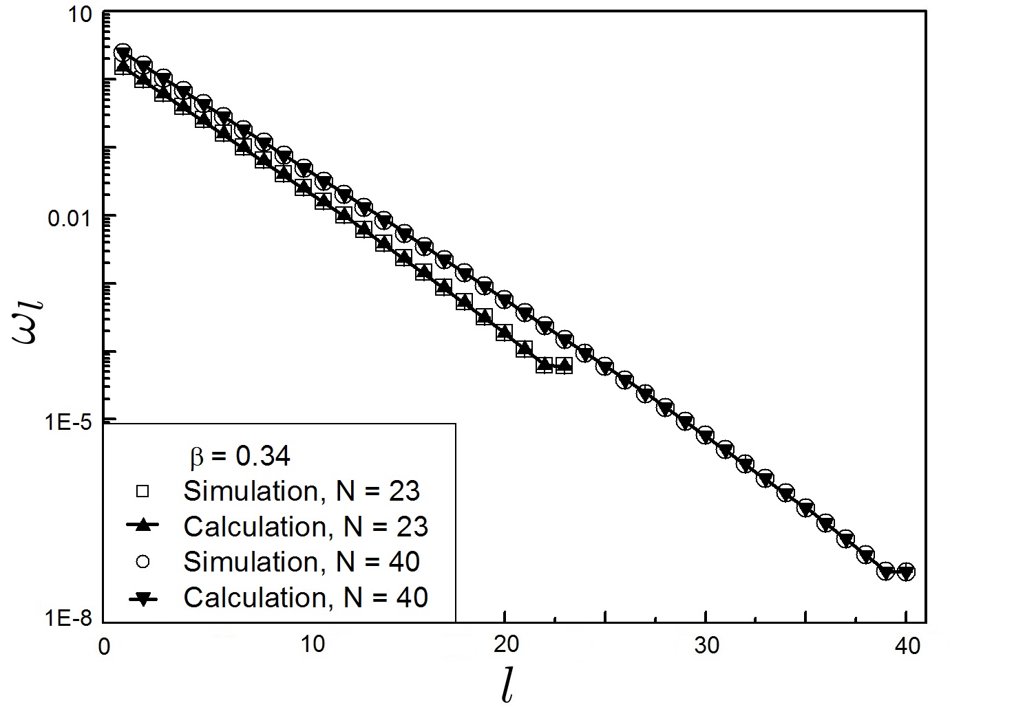
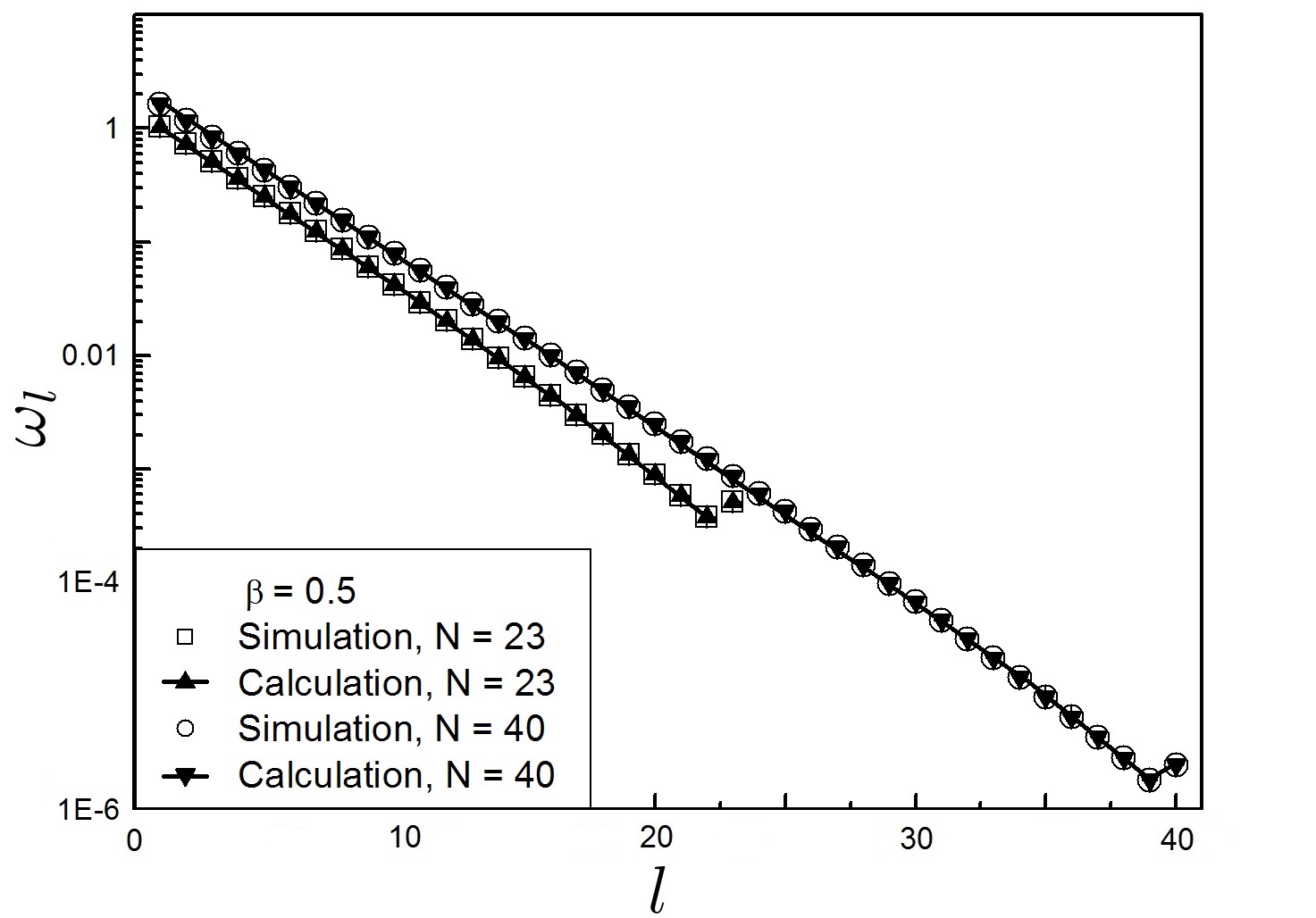
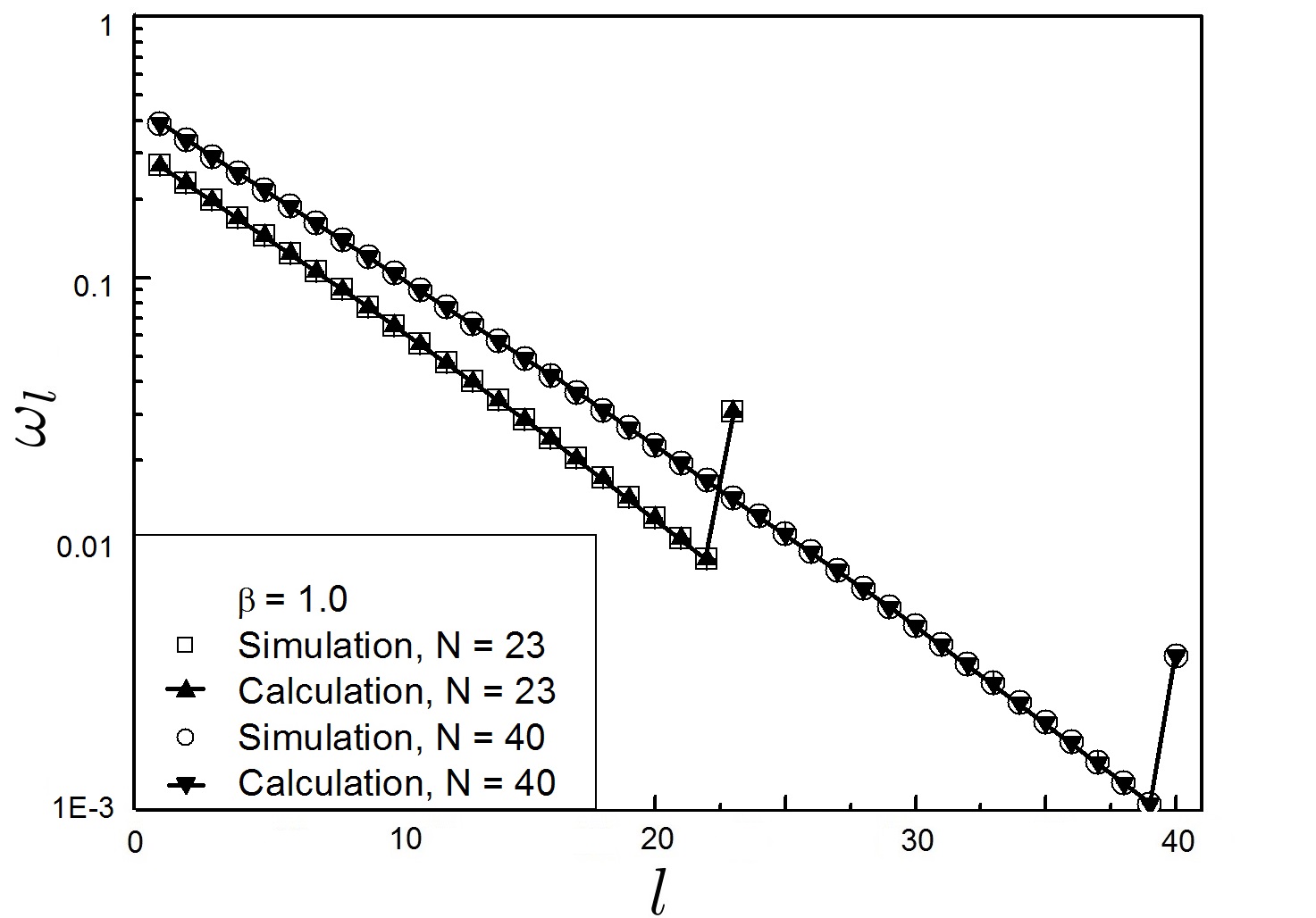
Figure 1: Cluster size distribution calculated using Eq. (9) (triangles) and found numerically for $N=23$ and $N=40$ (squares and circles) for three values of the lattice constant $\beta$. For $\beta=0.34<\beta_{c}$ (upper panel) $\omega_{l}$ monotonically decreases with the cluster size growth, while for $\beta=0.5>\beta_{c}$ (middle panel) and $\beta=1.0>\beta_{c}$ (lower panel) it has a maximum at $l=N$.

In order to demonstrate the occurrence of bimodality in the one dimensional Ising model we present here the results of our numerical simulations for the lattice sizes $N=23$ and $N=40$. These simulations were made using the Swendsen-Wang algorithm. For each run the first $5\cdot 10^{5}$ lattice configurations were discarded to ensure a complete thermalization, and the next $5\cdot 10^{7}$ lattice measurements were made while discarding every 5 lattice configurations between the measurements. For each measurement the total expectation of the number of clusters of all sizes was calculated, then the jackknife error analysis was used to obtain the error estimate of the mean values obtained.

Our numerical study includes 14 values of the lattice constant in the range from 0 to 2.5. We would like to stress that the coincidence of distribution functions simulated numerically and calculated according to formula (9) is perfect. In Fig. 1 the cluster size distribution is shown for three values of the lattice constant $\beta$. For $\beta=0.34<\beta_{c}$ the cluster size distribution is monotonic for both values of $N$. At the same time for the values of lattice constant above the “critical” one, i.e. for $\beta=0.5>\beta_{c}$ and for $\beta=1.0>\beta_{c}$, one can clearly see the bimodal distribution in Fig. 1. It is also seen that bimodality is enhanced with the lattice constant increasing. We have to remind once again that the present model does not have any phase transition in the thermodynamic limit. Hence, the one dimensional Ising model gives an explicit counterexample to treating bimodality as a signal of phase transition in finite systems.

IV Conclusions and perspectives

In this work we found an analytical solution of the one dimensional Ising model in terms of the geometrical clusters composed of the neighboring spins of the same direction. It is clear that the present formulation is an important step towards establishing a firm connection between the lattice spin systems and the statistical models of cluster type. The developed approach allows us to exactly calculate the size distribution of spin clusters for finite and infinite lattice sizes. Using the exact formulae we showed that for finite size of the lattice the one dimensional Ising model has a bimodal size distribution of clusters for $\beta>\ln 2/2$. We demonstrate that the bimodal size distribution of spin clusters in the present model is a finite size effect which appears due to a “condensation” of clusters whose size exceeds the lattice extent to the largest cluster. Such a “condensation” to the maximal cluster leads to the non-monotonic size distribution at sufficiently large values of the lattice constant in ferromagnetic case only. The obtained result is valid for all sizes of the lattice, however, in the thermodynamic limit it is washed out. It provides us with an explicit counterexample to the widely spread belief about an exclusive role of bimodality as a signal of phase transition in finite systems THill:1 ; Bmodal:Chomaz01 ; Bmodal:Chomaz03 ; Bmodal:Gulm04 ; Bmodal:Gulm07 . Our criticism is in full coherence with the results of Refs. CSMM ; Lopez ; Bmodal:Bugaev13 . The developed formalism considers the simplest exactly solvable lattice model, but it would be interesting to apply it to more realistic physical systems.

Acknowledgments. The authors appreciate the fruitful discussions with K. A. Bugaev and V. K. Petrov and their valuable comments. The work of A. I. I. is supported in part by the National Academy of Sciences of Ukraine Grant of GRID simulations for high energy physics.

References

- (1) D. H. E. Gross, Phys. Rep. 279, 119 (1997).
- (2) Ph. Chomaz, F. Gulminelli and V. Duflot, Phys. Rev. E, 64, 046114 (2001).
- (3) L. G. Moretto et al., Phys. Rev. Lett., 94, 202701 (2005).
- (4) K. A. Bugaev, Phys. Part. Nucl., 38, 447 (2007).
- (5) J. Natowitz et al., Phys. Rev. C, 65, 034618 (2002).
- (6) Pichon M. et al. (INDRA and ALADIN Collaborations), Nucl. Phys. A, 779, 267 (2006).
- (7) E. Bonnet et al. (INDRA and ALADIN Collaborations), Phys. Rev. Lett., 103, 072701 (2009).
- (8) S. Pratt, Physics 1, 29 (2008)
- (9) F. Karsch, PoSCPOD, 2013, 046 (046).
- (10) F. Gulminelli, Ph. Chomaz, Al. H. Raduta, and Ad. R. Raduta, Phys. Rev. E, 64, 046114 (2001).
- (11) Bugaev K. A., Acta. Phys. Polon., B 36, 3083 (2005).
- (12) K. A. Bugaev, A. I. Ivanytskyi, V. V. Sagun, D. R. Oliinychenko, Phys. Part. Nucl. Lett., 10, 832 (2013).
- (13) T. L. Hill, Thermodynamics of small systems, Dover, New York (1994).
- (14) Ph. Chomaz and F. Gulminelli, Physica A, 330, 451 (2003).
- (15) F. Gulminelli, Ann. Phys. Fr., 29, 6 (2004).
- (16) F. Gulminelli, Nucl. Phys. A, 791, 165 (2007).
- (17) C. N. Yang and T. D. Lee, Phys. Rev., 87, 404 (1952).
- (18) O. Lopez, D. Lacroix, and E. Vient, Phys. Rev. Lett., 95, 242701 (2005).
- (19) S. Das Gupta and A. Z. Mekjian, Phys. Rev. C, 57, 1361 (1998).
- (20) V. V. Sagun, A. I. Ivanytskyi, K. A. Bugaev and I. N. Mishustin, Nucl. Phys. A, 924, 4, 24 (2014).
- (21) E. Ising, Z. Phys., 31, 253 (1925).
- (22) M. E. Fisher, Physics, 3, 255 (1967).
- (23) A. Dillmann and G. E. Meier, J. Chem. Phys. 94, 3872 (1991).
- (24) A. Laaksonen, I. J. Ford, and M. Kulmala, Phys. Rev. E 49, 5517 (1994).
- (25) J. P. Bondorf et al., Phys. Rep., 257, 131 (1995).
- (26) J. I. Kapusta J. I., Phys. Rev. D, 23, 2444 (1981).
- (27) M. I. Gorenstein, G. M. Zinovjev and V. K. Petrov, Phys. Lett. B, 106, 327 (1981).
- (28) K. A. Bugaev, Phys. Rev. C, 76, 014903 (2007).
- (29) K. A. Bugaev, V. K. Petrov and G. M. Zinovjev, Phys. Part. Nucl. Lett., 9, 3, 238 (2012).
- (30) K. A. Bugaev, A. I. Ivanytskyi, E. G. Nikonov, V. K. Petrov, A. S. Sorin and G. M. Zinovjev, Phys. Atom. Nucl., 75, 6, 707 (2012).
- (31) I. Zakout, C. Greiner, J. Schaffner-Bielich, Nucl. Phys., A 781, 150 (2007).
- (32) I. Zakout, C. Greiner, Phys. Rev. C, 78, 034916 (2008).
- (33) L. Ferroni and V. Koch, Phys. Rev. C, 79, 034905 (2009).
- (34) L. G. Moretto et al., Phys. Rev. C, 68,1602 (2003) and references therein.
- (35) S. Fortunato and H. Satz, Phys. Lett. B, 475, 311 (2000).
- (36) S. Fortunato et. al, Phys. Lett. B, 502, 321 (2001).
- (37) C. Gattringer, Phys. Lett. B, 690, 179 (2010).
- (38) C. Gattringer and A. Schmidt, JHEP, 1101, 051 (2011.
- (39) G. Endrodi, A. Schäfer and J. Wellnhofer, arXiv:1506.07698 [hep-lat].
- (40) A. I. Ivanytskyi et. al., Physical properties of Polyakov loop geometrical clusters in gluodynamics (2015) (in preparation).