Householder QR Factorization With Randomization for Column Pivoting (HQRRP)

Abstract

A fundamental problem when adding column pivoting to the Householder QR factorization is that only about half of the computation can be cast in terms of high performing matrix-matrix multiplications, which greatly limits the benefits that can be derived from so-called blocking of algorithms. This paper describes a technique for selecting groups of pivot vectors by means of randomized projections. It is demonstrated that the asymptotic flop count for the proposed method is $2mn^{2}-(2/3)n^{3}$ for an $m\times n$ matrix, identical to that of the best classical unblocked Householder QR factorization algorithm (with or without pivoting). Experiments demonstrate acceleration in speed of close to an order of magnitude relative to the geqp3 function in LAPACK, when executed on a modern CPU with multiple cores. Further, experiments demonstrate that the quality of the randomized pivot selection strategy is roughly the same as that of classical column pivoting. The described algorithm is made available under Open Source license and can be used with LAPACK or libflame.

1 Introduction

The QR factorization is a staple of linear algebra, with applications ranging from Linear Least-Squares solution of overdetermined systems to the identification of low rank approximation via the determination of an approximate orthonormal basis for the column space. Standard algorithms for computing the QR factorization include Gram-Schmidt orthogonalization and those based on Householder transformations (reflectors). When it is desirable for the QR factorization to also reveal the approximate rank of the original matrix, it is important that the elements of the diagonal of $R$ be ordered with larger elements in magnitude appearing earlier. In this case, column pivoting (swapping) is employed during the QR factorization, yielding QR factorization with column pivoting (QRP). It is well-known that the Householder QR factorization (HQR) yields columns of $Q$ that are orthogonal to a high degree of precision, making these algorithms the weapon of choice in many situations. Pivoting can be added to HQR to yield HQR with column pivoting (HQRP). This topic is covered by standard texts on numerical linear algebra [13].

To achieve high performance for dense linear algebra algorithms, so-called blocked algorithms are employed that cast most computation in terms of matrix-matrix operations supported by the widely used level-3 Basic Linear Algebra Subprograms (BLAS) [7, 8] because such operations can be implemented to achieve very high performance on modern processors via a combination of careful reuse of data in the caches and low level implementation in terms of assembly code or intrinsic vector operations. Widely used current implementations of the level-3 BLAS are based on techniques exposed by Goto [15, 14] and available in open source libraries including the OpenBLAS [39] (a fork of the GotoBLAS) and BLIS [36], as well as vendor implementions including AMD’s ACML [2], Intel’s MKL [20], and IBM’s ESSL [19] libraries.

The fundamental problem with the classical approach to HQRP is that only half of the computation can be cast in terms of gemm, as described in the paper [31] that underlies LAPACK’s geqp3 routine [3]. This means that blocking can only improve performance by, at best, a factor two, which is inherent from the fact that it must be known how remaining columns will be updated in order to compute the 2-norms of remaining columns. Bischof and Quintana-Ortí describe in a pair of papers [5, 4] an attempt to overcome this problem by using so called “window pivoting” in combination with HQR. While much faster than geqp3, this approach is more complicated than the method proposed in this paper and never made it into LAPACK.

Fig. 1: Speedup of new blocked Householder QR factorization with randomized column pivoting (HQRRP) relative to LAPACK’s faster routine (dgeqp3) on a 14-core Intel Xeon E5-2695 v3, see Section 4.1 for details.

The present paper proposes to solve the problem by means of randomized projections. To describe the idea, suppose that we seek to determine a set of $b$ good pivot columns in an $m\times n$ matrix $A$. We then draw a Gaussian random matrix $G$ of size $b\times m$ and form a $b\times n$ sampling matrix $Y=GA$. Once $Y$ is available, we execute QRP on this matrix to find the $b$ pivot columns. This computation is efficient since $Y$ is small compared to $A$ (it has only $b$ rows), and results in good pivot choices since the random projection produces a matrix $Y$ that has approximately the same linear dependencies between its columns as does $A$. With this observation, it becomes easy to block the Householder QR factorization with column pivoting. At each iteration of the blocked algorithm, we use the randomized sampling approach to identify a set of $b$ columns that are then moved to the front of the actual matrix, at which point a regular step of HQR can be used to move the computation forward, optionally with additional column pivoting only within a narrow panel of the matrix. Importantly, the sampling matrix can be cheaply downdated rather than recomputed at each step, allowing the performance of the proposed algorithm to asymptotically approach that of a standard blocked HQR implementation that does not pivot columns. Fig. 1 illustrates the dramatic performance improvements that are realized.

The idea to use randomized sampling to pick blocks of pivot vectors was first published by Martinsson on ArXiv in May 2015 [28]. A very similar technique was published by Duersch and Gu in September 2015 [10], also on ArXiv. The observation that downdating of the sampling matrix enables the randomized scheme to attain the same asymptotic flop count as classical HQRP was discovered independently by the two groups and was first published in [10]. More broadly, the idea that one can select a subset of columns of a matrix that forms a good approximate basis for the column space of the matrix by performing QRP on a small matrix whose rows are random linear combinations of the rows of the original matrix was first described in [26, Sec. 4.1] and later elaborated in [23, 18, 27]. This problem is closely related to the problem of finding a set of columns of maximal spanning volume [16], and to the problem of finding so called CUR and interpolative decompositions [37]. These ideas tie in to a larger literature on randomized techniques for computing low-rank approximations of matrices that includes [12, 9, 24, 25].

This paper describes a practical implementation of the proposed method that can be incorporated in libraries like LAPACK and libflame [34, 35]. Implementation details that are important for attaining high practical performance are described to enable readers to reproduce and extend the ideas. The paper provides a cost analysis that shows that asymptotically the number of floating point operations approaches that of HQR without pivoting while most computation is cast in terms of matrix-matrix multiplication like the corresponding blocked HQR  without pivoting. It reports unprecedented performance for pivoted QR factorization on current architectures and provides empirical quality results. Importantly, the implementation is made available for use by the computational science community under an Open Source license. The conclusion discusses how these results pave the way for future opportunities.

The paper is organized as follows: Section 2 lists some standard facts about Householder reflectors and pivoted QR factorizations that we need in the presentation. Section 3 describes how the classical Householder QR factorization algorithm can be blocked by using randomization in the pivot selection step. Section 4 reports the results from numerical experiments investigating the speed of the algorithm and the quality of the pivoting selection strategy. Sections 5 summarizes the key results and discusses future work. Section 6 describes publicly available software that implements the techniques presented.

2 Householder QR Factorization

In this section, we briefly review the state-of-the art regarding Householder factorization based on Householder transformations (HQR). Throughout, we use the FLAME notation for representing dense linear algebra algorithms [30, 17]. In particular, for any matrix $X$, we let $m(X)$ and $n(X)$ denote the number of rows and columns of $X$, respectively.

2.1 Householder transformations (reflectors)

A standard topic in numerical linear algebra is the concept of a reflector, also known as a Householder transformation [13]. The review in this subsection follows [21] in which a similar notation is also employed.

Given a nonzero vector $u\in\mathbb{C}^{n}$, the matrix $H(u)=I-\frac{1}{\tau}uu^{H}$ with $\tau=\frac{u^{H}u}{2}$ has the property that it reflects a vector to which it is applied with respect to the subspace orthogonal to $u$. Given a vector $x$, the vector $u$ and scalar $\tau$ can be chosen so that $H(u)x$ equals a multiple of $e_{0}$, the first column of the identiy matrix. Furthermore, $u$ can be normalized so that its first element equals one.

In our discussions, given a vector $x=\left(\begin{array}[]{c}\chi_{1}\\ \hline\cr x_{2}\end{array}\right)$, the function $\left[\left(\begin{array}[]{c}\rho\\ \hline\cr u_{2}\end{array}\right),\tau\right]:={\rm Housev}\left(\left(\begin{array}[]{c}\chi_{1}\\ \hline\cr x_{2}\end{array}\right)\right)$ computes the vector $u=\left(\begin{array}[]{c}1\\ \hline\cr u_{2}\end{array}\right)$ and $\tau=\frac{u^{H}u}{2}$ so that $H(u)x=\rho e_{0}$,

2.2 Unblocked Householder QR factorization

A standard unblocked algorithm for HQR of a given matrix $A\in\mathbb{C}^{m\times n}$, typeset using the FLAME notation, is given in Fig. 2 (left). The body of the loop computes

$$\left[\left(\begin{array}[]{c}\rho_{11}\\ \hline\cr u_{21}\end{array}\right),\tau_{11}\right]:={\rm Housev}\left(\left(\begin{array}[]{c}\alpha_{11}\\ \hline\cr a_{21}\end{array}\right)\right),$$

which overwrites $a_{11}$ with $\rho_{11}$ and $a_{21}$ with $u_{21}$, after which the remainder of $A$ is updated by

$$\left(\begin{array}[]{c}a_{12}^{T}\\ \hline\cr A_{22}\end{array}\right):=\left(I-\frac{1}{\tau_{11}}\left(\begin{array}[]{c}1\\ \hline\cr u_{21}\end{array}\right)\left(\begin{array}[]{c}1\\ \hline\cr u_{21}\end{array}\right)^{H}\right)\left(\begin{array}[]{c}a_{12}^{T}\\ \hline\cr A_{22}\end{array}\right).$$

Upon completion, the (Householder) vectors that define the Householder transformations have overwritten the elements in which they introduced zeroes, and the upper triangular part of $A$ contains $R$. How the matrix $T$ fits into the picture will become clear next.

2.3 The UT transform: Accumulating Householder transformations

Given $A\in\mathbb{C}^{n\times b}$, let $U$ contain the Householder vectors computed during the HQR of $A$. Let us assume that $H(u_{b-1})\cdots H(u_{1})H(u_{0})A=R$. Then there exists an upper triangular matrix so that $I-UT^{-H}U^{H}=H(u_{b-1})\cdots H(u_{1})H(u_{0})$. The desired matrix $T$ equals the strictly upper triangular part of $U^{H}U$ with the diagonal elements equal to $\tau_{0},\ldots,\tau_{b-1}$. The matrix $T$ can be computed during the unblocked HQR, as indicated in Fig. 2 (left). In [21], the transformation $I-UT^{-1}U^{H}$ that equals the accumulated Householder transformations is called the UT transform. The UT transform is conceptually related to the more familiar WY transform [6] and compact WY transform [32], see [21] for details on how the different representations relate to one another.

2.4 A blocked QR Householder factorization algorithm

Algorithm:          $\left[A,T\right]:=\mbox{\sc HQR\_unb}(A,T)$ Partition $A\rightarrow\left(\begin{array}[]{c I c}A_{TL}\hfil\lx@intercol\vrule width=&A_{TR}\\ \cr\hline\cr\cr A_{BL}\hfil\lx@intercol\vrule width=&A_{BR}\end{array}\right)$ ,       $T\rightarrow\left(\begin{array}[]{c I c}T_{TL}\hfil\lx@intercol\vrule width=&T_{TR}\\ \cr\hline\cr\cr 0\hfil\lx@intercol\vrule width=&T_{BR}\end{array}\right)$ where $A_{TL}$ is $0\times 0$, $T_{TL}$ is $0\times 0$ while $m(A_{TL})<m(A)$ do   Determine  Repartition $\left(\begin{array}[]{c I c}A_{TL}\hfil\lx@intercol\vrule width=&A_{TR}\\ \cr\hline\cr\cr A_{BL}\hfil\lx@intercol\vrule width=&A_{BR}\end{array}\right)\rightarrow\left(\begin{array}[]{c I c | c}A_{00}\hfil\lx@intercol\vrule width=&a_{01}&A_{02}\\ \cr\hline\cr\cr a_{10}^{T}\hfil\lx@intercol\vrule width=&\alpha_{11}&a_{12}^{T}\\ \hline\cr A_{20}\hfil\lx@intercol\vrule width=&a_{21}&A_{22}\end{array}\right)$, $\left(\begin{array}[]{c I c}T_{TL}\hfil\lx@intercol\vrule width=&T_{TR}\\ \cr\hline\cr\cr 0\hfil\lx@intercol\vrule width=&T_{BR}\end{array}\right)\rightarrow\left(\begin{array}[]{c I c | c}T_{00}\hfil\lx@intercol\vrule width=&t_{01}&T_{02}\\ \cr\hline\cr\cr 0\hfil\lx@intercol\vrule width=&\tau_{11}&t_{12}^{T}\\ \hline\cr 0\hfil\lx@intercol\vrule width=&0&T_{22}\end{array}\right)$ where $\alpha_{11}$ is $1\times 1$, $\tau_{11}$ is $1\times 1$ $\begin{array}[]{l}\left[\left(\begin{array}[]{c}\alpha_{11}\\ \hline\cr a_{21}\end{array}\right),\tau_{11}\right]:={\rm Housev}\left(\begin{array}[]{c}\alpha_{11}\\ \hline\cr a_{21}\end{array}\right)\\ w_{12}^{T}:=(a_{12}^{T}+a_{21}^{H}A_{22})/\tau_{11}\\ \left(\begin{array}[]{c}a_{12}^{T}\\ \hline\cr A_{22}\end{array}\right):=\left(\begin{array}[]{c}a_{12}^{T}-{w_{12}^{T}}\\ \hline\cr A_{22}-{a_{21}}{w_{12}^{T}}\end{array}\right)\\ t_{01}:=(a_{10}^{T})^{H}+A_{20}^{H}a_{21}\\[23.84923pt] \end{array}$   Continue with $\left(\begin{array}[]{c I c}A_{TL}\hfil\lx@intercol\vrule width=&A_{TR}\\ \cr\hline\cr\cr A_{BL}\hfil\lx@intercol\vrule width=&A_{BR}\end{array}\right)\leftarrow\left(\begin{array}[]{c | c I c}A_{00}&a_{01}\hfil\lx@intercol\vrule width=&A_{02}\\ \hline\cr a_{10}^{T}&\alpha_{11}\hfil\lx@intercol\vrule width=&a_{12}^{T}\\ \cr\hline\cr\cr A_{20}&a_{21}\hfil\lx@intercol\vrule width=&A_{22}\end{array}\right)$, $\left(\begin{array}[]{c I c}T_{TL}\hfil\lx@intercol\vrule width=&T_{TR}\\ \cr\hline\cr\cr 0\hfil\lx@intercol\vrule width=&T_{BR}\end{array}\right)\leftarrow\left(\begin{array}[]{c | c I c}T_{00}&t_{01}\hfil\lx@intercol\vrule width=&T_{02}\\ \hline\cr 0&\tau_{11}\hfil\lx@intercol\vrule width=&t_{12}^{T}\\ \cr\hline\cr\cr 0&0\hfil\lx@intercol\vrule width=&T_{22}\end{array}\right)$ endwhile

Algorithm:          $\left[A,T\right]:=\mbox{\sc HQR\_blk}(A,T)$ Partition $A\rightarrow\left(\begin{array}[]{c I c}A_{TL}\hfil\lx@intercol\vrule width=&A_{TR}\\ \cr\hline\cr\cr A_{BL}\hfil\lx@intercol\vrule width=&A_{BR}\end{array}\right)$ , $T\rightarrow\left(\begin{array}[]{c}T_{T}\\ \cr\hline\cr\cr T_{B}\end{array}\right)$ where $A_{TL}$ is $0\times 0$, $T_{T}$ has $0$ rows while $m(A_{TL})<m(A)$ do   Determine block size $b$ Repartition $\left(\begin{array}[]{c I c}A_{TL}\hfil\lx@intercol\vrule width=&A_{TR}\\ \cr\hline\cr\cr A_{BL}\hfil\lx@intercol\vrule width=&A_{BR}\end{array}\right)\rightarrow\left(\begin{array}[]{c I c | c}A_{00}\hfil\lx@intercol\vrule width=&A_{01}&A_{02}\\ \cr\hline\cr\cr A_{10}\hfil\lx@intercol\vrule width=&A_{11}&A_{12}\\ \hline\cr A_{20}\hfil\lx@intercol\vrule width=&A_{21}&A_{22}\end{array}\right)$, $\left(\begin{array}[]{c}T_{T}\\ \cr\hline\cr\cr T_{B}\end{array}\right)\rightarrow\left(\begin{array}[]{c}T_{0}\\ \cr\hline\cr\cr T_{1}\\ \hline\cr T_{2}\end{array}\right)$ where $A_{11}$ is $b\times b$, $T_{1}$ has $b$ rows $\begin{array}[]{l}[\left(\begin{array}[]{c}A_{11}\\ \hline\cr A_{21}\end{array}\right),T_{1}]:=\\ ~{}~{}~{}~{}~{}\mbox{\sc HQR\_unb}(\left(\begin{array}[]{c}A_{11}\\ \hline\cr A_{21}\end{array}\right),T_{1})\\ W_{12}:=T_{1}^{-H}(U_{11}^{H}A_{12}+U_{21}^{H}A_{22})\\ \left(\begin{array}[]{c}A_{12}\\ \hline\cr A_{22}\end{array}\right):=\left(\begin{array}[]{c}A_{12}-U_{11}W_{12}\\ \hline\cr A_{22}-U_{21}W_{12}\end{array}\right)\\[-8.67204pt] {}\end{array}$   Continue with $\left(\begin{array}[]{c I c}A_{TL}\hfil\lx@intercol\vrule width=&A_{TR}\\ \cr\hline\cr\cr A_{BL}\hfil\lx@intercol\vrule width=&A_{BR}\end{array}\right)\leftarrow\left(\begin{array}[]{c | c I c}A_{00}&A_{01}\hfil\lx@intercol\vrule width=&A_{02}\\ \hline\cr A_{10}&A_{11}\hfil\lx@intercol\vrule width=&A_{12}\\ \cr\hline\cr\cr A_{20}&A_{21}\hfil\lx@intercol\vrule width=&A_{22}\end{array}\right)$, $\left(\begin{array}[]{c}T_{T}\\ \cr\hline\cr\cr T_{B}\end{array}\right)\leftarrow\left(\begin{array}[]{c}T_{0}\\ \hline\cr T_{1}\\ \cr\hline\cr\cr T_{2}\end{array}\right)$ endwhile

Fig. 2: Left: Unblocked Householder transformation based QR factorization merged with the computation of $T$ for the UT transform. Right: Blocked Householder transformation based QR factorization. In this algorithm, $U_{11}$ is the unit lower triangular matrix stored below the diagonal of $A_{11}$ and $U_{21}$ is stored in $A_{21}$.

A blocked algorithm for HQR that exploits the insights that resulted in the UT transform can now be described as follows. Partition

$$A\rightarrow\left(\begin{array}[]{c | c}A_{11}&A_{12}\\ \hline\cr A_{21}&A_{22}\end{array}\right)$$

where $A_{11}$ is $b\times b$. We can use the unblocked algorithm in Fig. 2 (left) to factor the panel $\left(\begin{array}[]{c}A_{11}\\ \hline\cr A_{21}\end{array}\right)$, creating matrix $T_{11}$ as a side effect. Now we need to also apply the UT transform to the rest of the columns:

$$\left(\begin{array}[]{c}A_{12}\\ \hline\cr A_{22}\end{array}\right) := \left(I-\left(\begin{array}[]{c}U_{11}\\ \hline\cr U_{21}\end{array}\right)T_{11}^{-1}\left(\begin{array}[]{c}U_{11}\\ \hline\cr U_{21}\end{array}\right)^{H}\right)^{H}\left(\begin{array}[]{c}A_{12}\\ \hline\cr A_{22}\end{array}\right)=\left(\begin{array}[]{c}A_{12}-U_{11}W_{12}\\ \hline\cr A_{22}-U_{21}W_{12}\end{array}\right),$$

where $W_{12}=T_{11}^{-H}(U_{11}^{H}A_{12}+U_{21}^{H}A_{22})$. This motivates the blocked HQR algorithm in Fig. 2 (right) which we will refer to as HQR_blk.

The benefit of the blocked algorithm is that it casts most computation in terms of the computations $U_{21}^{H}A_{22}$ (row panel times matrix multiply) and $A_{22}-U_{21}W_{12}$ (rank-$b$ update). Such matrix-matrix multiplications can attain high performance by amortizing data movement between memory layers.

These insights form the basis for the LAPACK routine geqrf (except that it uses a compact WY transform instead of the UT transform).

2.5 Householder QR factorization with column pivoting

An unblocked (rank-revealing) Householder QR factorization with column pivoting (HQRP) swaps the column of $A_{BR}$ with largest 2-norm with the first column of that matrix at the top of the loop body. As a result, the diagonal elements of matrix $R$ are ordered from largest to smallest in magnitude, which, for example, allows the resulting QR factorization to be used to identify a high quality approximate low-rank orthonormal basis for the column space of $A$. (To be precise, column pivoted QR returns a high quality basis in most cases but may produce strongly sub-optimal results in rare situations. For details, see [22, 16], and the description of “Matrix 4” in Section 4.2.)

The fundamental problem with the best known algorithm for HQRP, which underlies LAPACK’s routine geqp3, is that it only casts half of the computation in terms of matrix-matrix multiplication [31]. The unblocked algorithm called from the blocked algorithm operates on the entire “remaining matrix” ($A_{BR}$ in the blocked algorithm), computes $b$ more Householder transforms and $b$ more rows of $R$, computes the matrix $W_{2}$, and returns the information about how columns were swapped. In the blocked algorithm itself, only the update $A_{22}-A_{21}W_{2}$ remains to be performed. When only half the computation can be cast in terms of matrix-matrix multiplication, the resulting blocked algorithm is only about twice as fast as the unblocked algorithm.

3 Randomization to the Rescue

Algorithm: $\left[A,T,s\right]:=\mbox{\sc HQRP\_randomized\_blk}(A,T,s,b,p)$
$\begin{array}[]{@{}l}G:=\mbox{\sc rand\_iid}(b+p,n(A))\\ Y:=GA\\[-3.61371pt] \end{array}$
Partition $A\rightarrow\left(\begin{array}[]{c I c}A_{TL}\hfil\lx@intercol\vrule width=&A_{TR}\\ \cr\hline\cr\cr A_{BL}\hfil\lx@intercol\vrule width=&A_{BR}\end{array}\right)$ , $T\rightarrow\left(\begin{array}[]{c}T_{T}\\ \cr\hline\cr\cr T_{B}\end{array}\right)$ , $s\rightarrow\left(\begin{array}[]{c}s_{T}\\ \cr\hline\cr\cr s_{B}\end{array}\right)$ , $Y\rightarrow\left(\begin{array}[]{c I c}Y_{L}\hfil\lx@intercol\vrule width=&Y_{R}\end{array}\right)$ where $A_{TL}$ is $0\times 0$, $T_{T}$ has $0$ rows, $s_{T}$ has $0$ rows, $Y_{L}$ has $0$ columns
while $m(A_{TL})<m(A)$ do
Determine block size $b\rightarrow\min(b,n(A_{BR}))$ Repartition $\left(\begin{array}[]{c I c}A_{TL}\hfil\lx@intercol\vrule width=&A_{TR}\\ \cr\hline\cr\cr A_{BL}\hfil\lx@intercol\vrule width=&A_{BR}\end{array}\right)\rightarrow\left(\begin{array}[]{c I c | c}A_{00}\hfil\lx@intercol\vrule width=&A_{01}&A_{02}\\ \cr\hline\cr\cr A_{10}\hfil\lx@intercol\vrule width=&A_{11}&A_{12}\\ \hline\cr A_{20}\hfil\lx@intercol\vrule width=&A_{21}&A_{22}\end{array}\right)$, $\left(\begin{array}[]{c}T_{T}\\ \cr\hline\cr\cr T_{B}\end{array}\right)\rightarrow\left(\begin{array}[]{c}T_{0}\\ \cr\hline\cr\cr T_{1}\\ \hline\cr T_{2}\end{array}\right)$ , $\left(\begin{array}[]{c}s_{T}\\ \cr\hline\cr\cr s_{B}\end{array}\right)\rightarrow\left(\begin{array}[]{c}s_{0}\\ \cr\hline\cr\cr s_{1}\\ \hline\cr s_{2}\end{array}\right)$ , $\left(\begin{array}[]{c I c}Y_{L}\hfil\lx@intercol\vrule width=&Y_{R}\end{array}\right)\rightarrow\left(\begin{array}[]{c I c | c}Y_{0}\hfil\lx@intercol\vrule width=&Y_{1}&Y_{2}\end{array}\right)$ where $A_{11}$ is $b\times b$, $T_{1}$ has $b$ rows, $s_{1}$ has $b$ rows, $Y_{1}$ has $b$ columns
$\begin{array}[]{l}s_{1}:=\mbox{\sc DeterminePivots}(\left(\begin{array}[]{c | c}Y_{1}&Y_{2}\end{array}\right),b)\\ \left(\begin{array}[]{c | c}A_{01}&A_{02}\\ \cr\hline\cr\cr A_{11}&A_{12}\\ \hline\cr A_{21}&A_{22}\end{array}\right):=\mbox{\sc SwapCols}(s_{1},\left(\begin{array}[]{c | c}A_{01}&A_{02}\\ \cr\hline\cr\cr A_{11}&A_{12}\\ \hline\cr A_{21}&A_{22}\end{array}\right))\\ \left[\left(\begin{array}[]{c}A_{11}\\ \hline\cr A_{21}\end{array}\right),T_{1}{\color[rgb]{0,0,0}\hbox{\pagecolor{white}$,s_{1}^{\prime}$}}\right]:=\mbox{\sc HQR{\color[rgb]{0,0,0} \hbox{\pagecolor{white}\sc P}}\_unb}(\left(\begin{array}[]{c}A_{11}\\ \hline\cr A_{21}\end{array}\right),T_{1})\\ {\color[rgb]{0,0,0}A_{01}:=\mbox{\sc SwapCols}(s_{1}^{\prime},A_{01})}\\ {\color[rgb]{0,0,0}s_{1}:=\mbox{\sc UpdatePivotInfo}(s_{1}^{\prime},s_{1})}\\ W_{12}:=T_{1}^{-H}(U_{11}^{H}A_{12}+U_{21}^{H}A_{22})\\ \left(\begin{array}[]{c}A_{12}\\ \hline\cr A_{22}\end{array}\right):=\left(\begin{array}[]{c}A_{12}-U_{11}W_{12}\\ \hline\cr A_{22}-U_{21}W_{12}\end{array}\right)\\ \left(\begin{array}[]{c | c}Y_{1}&Y_{2}\end{array}\right):=\mbox{\sc SwapCols}(s_{1},\left(\begin{array}[]{c | c}Y_{1}&Y_{2}\end{array}\right))\\ Y_{2}:=Y_{2}-\left(G_{1}-(G_{1}U_{11}+G_{2}{U_{21}})T_{11}^{-1}{U_{11}}^{H}\right){R_{12}}.\end{array}$
Continue with $\left(\begin{array}[]{c I c}A_{TL}\hfil\lx@intercol\vrule width=&A_{TR}\\ \cr\hline\cr\cr A_{BL}\hfil\lx@intercol\vrule width=&A_{BR}\end{array}\right)\leftarrow\left(\begin{array}[]{c | c I c}A_{00}&A_{01}\hfil\lx@intercol\vrule width=&A_{02}\\ \hline\cr A_{10}&A_{11}\hfil\lx@intercol\vrule width=&A_{12}\\ \cr\hline\cr\cr A_{20}&A_{21}\hfil\lx@intercol\vrule width=&A_{22}\end{array}\right)$, $\left(\begin{array}[]{c}T_{T}\\ \cr\hline\cr\cr T_{B}\end{array}\right)\leftarrow\left(\begin{array}[]{c}T_{0}\\ \hline\cr T_{1}\\ \cr\hline\cr\cr T_{2}\end{array}\right)$ , $\left(\begin{array}[]{c}s_{T}\\ \cr\hline\cr\cr s_{B}\end{array}\right)\leftarrow\left(\begin{array}[]{c}s_{0}\\ \hline\cr s_{1}\\ \cr\hline\cr\cr s_{2}\end{array}\right)$ , $\left(\begin{array}[]{c I c}Y_{L}\hfil\lx@intercol\vrule width=&Y_{R}\end{array}\right)\leftarrow\left(\begin{array}[]{c | c I c}Y_{0}&Y_{1}\hfil\lx@intercol\vrule width=&Y_{2}\end{array}\right)$
endwhile

Fig. 3: Blocked Householder transformation based QR factorization with column pivoting based on randomization. In this algorithm, $U_{11}$ equals the unit lower triangiular matrix stored below the diagonal of $A_{11}$, $U_{21}=A_{21}$, and $R_{12}=A_{12}$. The steps highlighted in gray constitute the blocked QR factorization without column pivoting from Fig. 2.

This section describes a computationally efficient technique for picking a selection of $b$ columns from a given $n\times n$ matrix $A$ that form good choices for the first $b$ pivots in a blocked HQRP algorithm. Observe that this task is closely related to the problem of finding an index set $s$ of length $b$ such that the columns in $A(:,s)$ form a good approximate basis for the column space of $A$. Another way of expressing this problem is that we are looking for a collection of $b$ columns whose spanning volume in $\mathbb{C}^{n}$ is close to maximal. To find the absolutely optimal choice here is a hard problem [16], but luckily, for pivoting purposes it is sufficient to find a choice that is “good enough.”

3.1 Randomized pivot selection

The strategy that we propose is simple. The idea is to perform classical QR factorization with column pivoting (QRP) on a matrix $Y$ that is much smaller than $A$, so that performing QRP with that matrix constitutes a lower order cost. As a bonus, it may fit in fast cache memory. This smaller matrix can be constructed by forming random linear combinations of the rows of $A$ as follows:

1. Fix an over-sampling parameter $p$. Setting $p=5$ or $p=10$ are good choices.

2. Form a random matrix $G$ of size $(b+p)\times n$ whose entries are drawn independently from a normalized Gaussian distribution.

3. Form the $(b+p)\times n$ sampling matrix $Y=GA$.

The sampling matrix $Y$ has as many columns as $A$, but many fewer rows. Now execute $b$ steps of a column pivoted QR factorization to determine an integer vector with $b$ elements that capture how columns need to be pivoted:

$$s=\mbox{\sc DeterminePivots}(Y,b).$$

In other words, the columns $Y(:,s)$ are good pivot columns for $Y$. Our claim is that due to the way $Y$ is constructed, the columns $A(:,s)$ are then also good choices for pivot columns of $A$. This claim is supported by extensive numerical experiments, some of which are given in Section 4.2. There is theory supporting the claim that these $b$ columns form a good approximate basis for the column space of $A$, see, e.g. [18, Sec. 5.2] and [23, 37], but it has not been directly proven that they form good choices as pivots in a QR factorization. This should not be surprising given that it is known that even classical column pivoting can result in poor choices [22]. Known algorithms that are provably good are all far more complex to implement [16].

Notice that there are many choices of algorithms that can be employed to determine the pivots. For example, since high numerical accuracy is not necessary, the classical Modified Gram-Schmidt (MGS) algorithm with column pivoting is a simple yet effective choice.

The randomized strategy described here for determining a block of pivot vectors is inspired by a technique published in [26, Sec. 4.1] for computing a low-rank approximation to a matrix, and later elaborated in [23, 18, 27].

Remark 1 (Choice of over-sampling parameter $p$).

The reliability of the procedures described in this section depends on the choice of the over-sampling parameter $p$. It is well understood how large $p$ needs to be in order to determine a high-quality approximate basis for the column space of $A$ with extremely high reliability: the choice $p=5$ is very good, $p=10$ is excellent, and $p=b$ is almost always over-kill [18]. The pivot selection problem is less well studied, but is more forgiving. (The choice of pivots does not necessarily have to be particularly optimal.) Numerical experiments indicate that even setting $p=0$ typically results in good choices. However, the choices $p=5$ or $p=10$ appear to be good generic values that have resulted in excellent choices in every experiment we have run.

Remark 2 (Intuition of random projections).

To understand why the pivot columns selected by processing the small matrix $Y$ also form good choices for the original matrix $A$, it might be helpful to observe that for a Gaussian random matrix $G$ of size $\ell\times n$, it is the case that for any $x\in\mathbb{R}^{n}$, we have $\mathbb{E}\bigl{[}\|Gx\|^{2}\bigr{]}=\|x\|^{2}$, where $\mathbb{E}$ denotes expectation. Moreover, as the number of rows $\ell$ grows, the probability distribution of $\|Gx\|$ concentrates tightly around its expected value, see, e.g., [38, Sec. 2.4] and the references therin. This means that for any pair of indices $i,j\in\{1,2,\dots,n\}$ we have $\mathbb{E}\bigl{[}\|Y(:,i)-Y(:,j)\|^{2}\bigr{]}=\|A(:,i)-A(:,j)\|^{2}$. This simple observation does not in any way provide a proof that the randomized strategy we propose works, but might help understand the underlying intuition.

3.2 Efficient downdating of the sampling matrix $Y$

For the QRP factorization algorithm, it is well known that one does not need to recompute the column norms of the remainder matrix after each step. Instead, these can be cheaply downdated, as described, e.g., in [33, Ch.5, Sec. 2.1]. In terms of asymptotic flop counts, this observation makes the cost of pivoting become a lower order term, and consequently both unpivoted and pivoted Householder QR algorithms have the same leading order term $(4/3)n^{3}$ in their asymptotic flop counts for $n\times n$ matrices. In this section, we describe an analogous technique for the randomized sampling strategy described in Section 3.1. This downdating strategy was discovered by one of the authors; a closely related technique was discovered independently and published to arXiv by Duersch and Gu [10] in September 2015.

First observe that if the randomized sampling technique described in Section 3.1 is used in the obvious fashion, then each step of the iteration requires the generation of a Gaussian random matrix $G$ and a matrix-matrix multiply involving the remaining portion of $A$ in the lower right corner to form the sampling matrix $Y$. The number of flops required by the matrix-matrix multiplications add up to an $O(n^{3})$ term for $n\times n$ matrices. However, it turns out to be possible to avoid computing a sampling matrix $Y$ from scratch at every step. The idea is that if we select the randomizing matrix $G$ in a particular way in every step beyond the first, then the corresponding sampling matrix $Y$ can inexpensively be computed by downdating the sampling matrix from the previous step.

To illustrate, suppose that we start with an $n\times n$ original matrix $A=A^{(0)}$. In the first blocked step, we draw a $(b+p)\times n$ randomizing matrix $G^{(1)}$ and form the $(b+p)\times n$ sampling matrix

$$Y^{(1)}=G^{(1)}A^{(0)}.$$ (2)

Using the information in $Y^{(1)}$, we identify the $b$ pivot vectors and form the corresponding permutation matrix $P^{(1)}$. Then the matrix $Q^{(1)}$ representing the $b$ Householder reflectors dictated by the $b$ pivot columns is formed. Applying these transforms to the right and the left of $A^{(0)}$, we obtain the matrix

$$A^{(1)}=\bigl{(}Q^{(1)}\bigr{)}^{*}A^{(0)}P^{(1)}.$$ (3)

To select the pivots in the next step, we need to form a randomizing matrix $G^{(2)}$ and a sampling matrix $Y^{(2)}$ that are related through

$$Y^{(2)}=G^{(2)}\bigl{(}A^{(1)}-R^{(1)}\bigr{)},$$ (4)

where $R^{(1)}$ holds the top $b$ rows of $A^{(1)}$ so that

$$A^{(1)}-R^{(1)}=\left(\begin{array}[]{cc}A_{11}^{(1)}&A_{12}^{(1)}\\ 0&A_{22}^{(1)}\end{array}\right)-\left(\begin{array}[]{cc}A_{11}^{(1)}&A_{12}^{(1)}\\ 0&0\end{array}\right)=\left(\begin{array}[]{cc}0&0\\ 0&A_{22}^{(1)}\end{array}\right).$$

The key idea is now to choose the randomizing matrix $G^{(2)}$ according to the formula

$$G^{(2)}=G^{(1)}Q^{(1)}.$$ (5)

Inserting (5) into (4), we now find that the sampling matrix is

$$Y^{(2)}=G^{(1)}Q^{(1)}\bigl{(}A^{(1)}-R^{(1)}\bigr{)}=\{\mbox{Use (\ref{eq:idea2})}\}=\\ G^{(1)}A^{(0)}P^{(1)}-G^{(1)}Q^{(1)}R^{(1)}=\{\mbox{Use (\ref{eq:idea1})}\}=Y^{(1)}P^{(1)}-G^{(1)}Q^{(1)}R^{(1)}.$$ (6)

Evaluating formula (6) is inexpensive since the first term is a permutation of the columns of the sampling matrix $Y^{(1)}$ and the second term is a product of thin matrices (recall that $Q^{(1)}$ is a product of $b$ Householder reflectors).

Remark 3.

Since the probability distribution for Gaussian random matrices is invariant under unitary maps, the formula (5) appears quite safe. After all, $G^{(1)}$ is Gaussian, and $Q^{(1)}$ is just a sequence of reflections, so it might be tempting to conclude that the new randomizing matrix must be Gaussian too. However, the matrix $Q^{(1)}$ unfortunately depends on the draw of $G^{(1)}$, so this argument does not work. Nevertheless, the dependence of $Q^{(1)}$ on $G^{(1)}$ is very subtle since this $Q^{(1)}$ is dictated primarily by the directions of the good pivot columns. Extensive practical experiments (see, e.g., Section 4.2) indicate that the pivoting strategy described in this section based on downdating is just as good as the one that uses “pure” Gaussian matrices that was described in Section 3.1.

3.3 Detailed description of the downdating procedure

Having described the downdating procedure informally in Section 3.2, we in this section provide a detailed description using the notation for HQR that we used in Section 3. First, let us assume that one iteration of the blocked algorithm has completed, so that, at the bottom of the loop body, the matrix $A$ contains

$$\left(\begin{array}[]{c | c}A_{11}&A_{12}\\ \hline\cr A_{21}&A_{22}\end{array}\right)=\left(\begin{array}[]{c | c}{U\backslash R}_{11}&R_{12}\\ \hline\cr U_{21}&\widehat{A}_{22}-U_{21}W_{12}\end{array}\right).$$

Here $\widehat{A}$ denotes the original contents of $AP_{1}$, where $P_{1}$ captures how columns have been swapped so far. Hence, cf. (3),

$$\begin{array}[t]{c}\underbrace{\left(I-\left(\begin{array}[]{c}U_{11}\\ \hline\cr U_{21}\end{array}\right)T_{11}^{-H}\left(\begin{array}[]{c}U_{11}\\ \hline\cr U_{21}\end{array}\right)^{H}\right)}\\ {\color[rgb]{0,0,0}\left(\begin{array}[]{c | c}Q_{1}&Q_{2}\end{array}\right)}\end{array}\left(\begin{array}[]{c | c}\widehat{A}_{11}&\widehat{A}_{12}\\ \hline\cr\widehat{A}_{21}&\widehat{A}_{22}\end{array}\right)P_{1}=\left(\begin{array}[]{c | c}R_{11}&R_{12}\\ \hline\cr 0&A_{22}\end{array}\right)$$

Now, let $\widetilde{G}_{2}$ be the next sampling matrix and $\widetilde{Y}_{2}=\widetilde{G}_{2}A_{22}$. In order to show how this new sampling matrix can be computed by downdating the last sampling matrix, consider that

$$\left(\begin{array}[]{c | c}\widetilde{Y}_{1}&\widetilde{Y}_{2}\end{array}\right)=\left(\begin{array}[]{c | c}\widetilde{G}_{1}&\widetilde{G}_{2}\end{array}\right)\left(\begin{array}[]{c | c}0&0\\ \hline\cr 0&A_{22}\end{array}\right)$$

for some matrix $\widetilde{G}_{1}$ and that

$$\@ADDCLASS{ltx_eqn_lefteqn}$\displaystyle\left(\begin{array}[]{c | c}\widetilde{G}_{1}&\widetilde{G}_{2}\end{array}\right)\left(\begin{array}[]{c | c}0&0\\ \hline\cr 0&A_{22}\end{array}\right)=\left(\begin{array}[]{c | c}\widetilde{G}_{1}&\widetilde{G}_{2}\end{array}\right)\left(\left(\begin{array}[]{c | c}R_{11}&R_{12}\\ \hline\cr 0&A_{22}\end{array}\right)-\left(\begin{array}[]{c | c}R_{11}&R_{12}\\ \hline\cr 0&0\end{array}\right)\right)$\mbox{}\hfil\\ =\left(\begin{array}[]{c | c}\widetilde{G}_{1}&\widetilde{G}_{2}\end{array}\right)\left(\begin{array}[]{c | c}R_{11}&R_{12}\\ \hline\cr 0&A_{22}\end{array}\right)-\left(\begin{array}[]{c | c}\widetilde{G}_{1}&\widetilde{G}_{2}\end{array}\right)\left(\begin{array}[]{c | c}{R}_{11}&R_{12}\\ \hline\cr 0&0\end{array}\right)\\ =\left(\begin{array}[]{c | c}\widetilde{G}_{1}&\widetilde{G}_{2}\end{array}\right)\left(\begin{array}[]{c | c}Q_{1}&Q_{2}\end{array}\right)\widehat{A}P_{1}-\left(\begin{array}[]{c | c}\widetilde{G}_{1}&\widetilde{G}_{2}\end{array}\right)\left(\begin{array}[]{c | c}Q_{1}&Q_{2}\end{array}\right)\left(\begin{array}[]{c | c}Q_{1}&Q_{2}\end{array}\right)^{H}\left(\begin{array}[]{c | c}{R}_{11}&R_{12}\\ \hline\cr 0&0\end{array}\right)$$ (7)

The choice of randomizing matrix analogous to (5) is now

$$\left(\begin{array}[]{c | c}\widetilde{G}_{1}&\widetilde{G}_{2}\end{array}\right)=\left(\begin{array}[]{c | c}G_{1}&G_{2}\end{array}\right)\left(\begin{array}[]{c | c}Q_{1}&Q_{2}\end{array}\right).$$ (8)

Inserting the choice (8) into (7), we obtain

$$\left(\begin{array}[]{c | c}\widetilde{Y}_{1}&\widetilde{Y}_{2}\end{array}\right)=\begin{array}[t]{c}\underbrace{\left(\begin{array}[]{c | c}G_{1}&G_{2}\end{array}\right)\widehat{A}}\\ \left(\begin{array}[]{c | c}Y_{1}&Y_{2}\end{array}\right)\end{array}P_{1}-\left(\begin{array}[]{c | c}G_{1}&G_{2}\end{array}\right)\left(I-\left(\begin{array}[]{c}U_{11}\\ \hline\cr U_{21}\end{array}\right)T_{11}^{-H}\left(\begin{array}[]{c}U_{11}\\ \hline\cr U_{21}\end{array}\right)^{H}\right)^{H}\left(\begin{array}[]{c | c}{R}_{11}&R_{12}\\ \hline\cr 0&0\end{array}\right).$$

Letting $\left(\begin{array}[]{c | c}\overline{Y}_{1}&\overline{Y}_{2}\end{array}\right)=\left(\begin{array}[]{c | c}Y_{1}&Y_{2}\end{array}\right)P_{1}$ we conclude that

$$\widetilde{Y}_{2} = \overline{Y}_{2}-\left(\begin{array}[]{c | c}G_{1}&G_{2}\end{array}\right)\left(I-\left(\begin{array}[]{c}U_{11}\\ \hline\cr U_{21}\end{array}\right)T_{11}^{-1}\left(\begin{array}[]{c}U_{11}\\ \hline\cr U_{21}\end{array}\right)^{H}\right)\left(\begin{array}[]{c}R_{12}\\ \hline\cr 0\end{array}\right)$$

$$= \overline{Y}_{2}-\left(\begin{array}[]{c | c}G_{1}&G_{2}\end{array}\right)\left(\left(\begin{array}[]{c}R_{12}\\ \hline\cr 0\end{array}\right)-\left(\begin{array}[]{c}U_{11}\\ \hline\cr U_{21}\end{array}\right)T_{11}^{-1}{U_{11}}^{H}R_{12}\right)$$

$$= \overline{Y}_{2}-\left(G_{1}-(G_{1}U_{11}+G_{2}{U_{21}})T_{11}^{-1}{U_{11}}^{H}\right){R_{12}}.$$

which can then be used to downdate the sampling matrix $Y$.

3.4 The blocked algorithm

In Fig. 3, we give the blocked algorithm that results when the randomized pivot selection strategy described in Section 3.1 is combined with the downdating techniques described in Section 3.3. In that figure, there is a call to a function “HRQP_UNB” which is an unblocked HQR algorithm with column pivoting. The purpose of this call is to factor the current column panel so that the diagonal elements within blocks on the diagonal of $R$ are ordered from largest to smallest in magnitude. Moreover, the call to “UpdatePivotInfo” takes the pivoting that occurred within the current panel (to ensure strictly decreasing diagonal elements within the current diagonal block of $R_{11}$) and merges this with the pivot information that occurred when determining the columns to be moved into that current panel.

3.5 Asymptotic cost analysis

In analyzing the asymptotic complexity of the method, we consider a matrix of size $m\times n$, with $m\geq n$. We assume that the block size $b$ and the over-sampling parameter $p$ are kept fixed as $m$ and $n$ grow. We first note that all steps in Fig. 3 highlighted in grey are part of the blocked HQR algorithm, which is known to have an asymptotic cost of $2mn^{2}-2/3n^{3}$ flops. This leaves us to discuss the overhead related to the other operations.

• $G:=\mbox{\sc rand\_iid}(b+p,m)$: Cost: ignored.

• $Y:=GA$: Cost: $O((b+p)mn)$ flops.

• $s_{1}:=\mbox{\sc DeterminePivots}(\left(\begin{array}[]{c | c}Y_{1}&Y_{2}\end{array}\right),b)$: Cost: $O(b(b+p)(n-kb))$ flops during the $k$th iteration of the blocked algorithm, for a total of $O((b+p)n^{2})$ flops. (Recall that the factorization of this matrix can stop after the first $b$ columns have been identified.)

• $\cdots:=\mbox{\sc SwapCols}(s_{1},\cdots)$: Cost: ignored.

• $Y_{2}:=Y_{2}-\left(G_{1}-(G_{1}U_{11}+G_{2}{U_{21}})T_{11}^{-1}{U_{11}}^{H}\right){R_{12}}$: Aggregate cost: $O((b+p)n^{2})$.

Thus, the overhead is $O((b+p)(n^{2}+mn))$ flops and the total cost is

$$2mn^{2}-2/3n^{3}+O((b+p)(n^{2}+mn))\mbox{ flops},$$

which, asymptotically, approaches the same $2mn^{2}-2/3n^{3}$ cost as unpivoted HQR.

4 Experiments

This section describes the results from two sets of experiments. Section 4.1 compares the computational speed of the proposed scheme to existing state-of-the-art methods for computing column pivoted QR factorizations. Section 4.2 investigates how well the proposed randomized technique works at selecting pivot columns. Specifically, we investigate how well the rank-$k$ truncated QR factorization approximates the original matrix and compare the results to those obtained by classical column pivoting.

4.1 Performance experiments

We have implemented the proposed HQRRP algorithm using the libflame [35, 34] library that allows our implementations to closely resemble the algorithms as presented in the paper.

Platform details. All experiments reported in this article were performed on an Intel Xeon E5-2695 v3 (Haswell) processor (2.3 GHz), with 14 cores. In order to be able to show scalability results, the clock speed was throttled at 2.3 GHz, turning off so-called turbo boost. Each core can execute 16 double precision floating point operations per cycle, meaning that the peak performance of one core is 36.8 GFLOPS (billions of floating point operations per second). For comparison, on a single core, dgemm achieves around 33.6 GFLOPS. Other details of interest include that the OS used was Linux (Version 2.6.32-504.el6.x86_64), the code was compiled with gcc (Version 4.4.7), dgeqrf and dgeqp3 were taken from LAPACK (Release 3.4.0), and the implementations were linked to BLAS from Intel’s MKL library (Version 11.2.3). Our implementations were coded with libflame (Release 11104).

Implementations. We report performance for four implementations:

dgeqrf. The implementation of blocked HQR that is part of the netlib implemenation of LAPACK, modified so that the block size can be controlled.

dgeqp3. The implementation of blocked HQRP that is part of the netlib implemenation of LAPACK, based on [31], modified so that the block size can be controlled.

HQRRPbasic. Our implementation of HQRRP that computes new matrices $G$ and $Y$ in every iteration. This implementation deviates from the algorithm in Fig. 3 in that it also incorporates additional column pivoting within the call to HQRRP_unb.

HQRRP. The implementation of HQRRP that downdates $Y$. (It also includes pivoting within HQRRP_unb).

dgeqpx. An implementation of HQRP with window pivoting [5, 4], briefly mentioned in the introduction. This algorithm consists of two stages: The first stage is a QR with window pivoting. An incremental condition estimator is employed to accept/reject the columns within a window. The size of the window is about about twice the block size used by the algorithm to maintain locality. If all the columns in the window are unacceptable, all of them are rejected and fresh ones are brought into the window. The second stage is a postprocessing stage to validate the rank, that is, to check that all good columns are in the front, and all the bad columns are in the rear. This step is required because the window pivoting could fail to reveal the rank due to its shortsightedness (having only checked the window and having employed a cheap to compute condition estimator.) Sometimes, some columns must be moved between $R_{11}$ that has been computed and matrices $R_{12}$ and $R_{22}$, and then retriangularization must be performed with Givens rotations.

In all cases, we used algorithmic block sizes of $b=64$ and $128$. While likely not optimal for all problem sizes, these blocks sizes yield near best performance and, regardless, it allows us to easily compare and contrast the performance of the different implementations.

Fig. 4: Computational speed (in standardized Gigaflops) of the proposed randomized algorithm HQRRP for computing a column pivoted QR-factorization of a matrix of size $n\times n$. The four graphs show results from test runs on 1, 4, 8, and 14 cores on an Intel Xeon E5-2695 v3. Observe that the scales on the vertical axes are different in the four graphs. For comparison, the graphs also show the times for competing algorithms (dgeqp3 and dgeqpx), and for unpivoted QR (dgeqrf), see Section 4.1 for details. The proposed algorithm HQRRP is faster than competing algorithms, with the gap growing as more cores are added. The block size for all algorithms was set to $b=64$. Figure 1 shows the relative speeds in detail.

Fig. 5: Computational speeds (in standardized Gigaflops) for the same problem as that shown in Figure 4. In this figure, results are shown for a blocksize of $b=128$, in contrast with the blocksize $b=64$ that was used in Figure 4.

Results. As is customary in these kinds of performance comparisons, we compute the achieved performance as

$$\frac{4/3n^{3}}{\mbox{time (in sec.)}}\times 10^{-9}\mbox{ GFLOPS}.$$

Thus, even for the implementations that perform more computations, we only count the floating point operations performed by an unblocked HQR without pivoting.

Figure 4 reports performance on 1, 4, 8, and 14 cores. We see that HQRRP handily outperforms dgeqp3 and to a lesser degree also outperforms dgeqpx. Moreover, the asymptotic performance of HQRRP appears to approach that of dgeqrf, in particular for the single core case. We also see that while the relative performances of all 5 methods remain qualitatively the same across the four graphs, it is clear that as the number of cores grows, the speed advantage of HQRRP over dgeqp3 becomes even further pronounced, cf. Figure 1.

Figure 4 also shows that while the absolute speed of all five algorithms studied improves as the number of cores grows, all five fall substantially short of ideal scaling (in that the number of Gigaflops per core falls as the number of cores grows). This observation underscores the need for further research in this area.

In order to investigate the effect of the block size on the computational speed, we reran the experiments shown in Figure 4 with a block size of $b=128$ instead of $b=64$, with the results shown in Figure 5. We see that the choice $b=64$ tends to lead to slightly faster execution, but the key take-away from this comparison is that the speed is relatively insensitive to the precise choice of block size (within reason, of course).

4.2 Quality experiments

In this section, we describe the results of numerical experiments that were conducted to compare the quality of the pivot choices made by our randomized algorithm HQRRP to those resulting from classical column pivoting. Specifically, we compared how well partial factorizations reveal the numerical ranks of four different test matrices:

• Matrix 1 (fast decay): This is an $n\times n$ matrix of the form $A=UDV^{*}$ where $U$ and $V$ are randomly drawn matrices with orthonormal columns (obtained by performing QR on a random Gaussian matrix), and where $D$ is diagonal with entries given by $d_{j}=\beta^{(j-1)/(n-1)}$ with $\beta=10^{-5}$.

• Matrix 2 (S shaped decay): This matrix is built in the same manner as “Matrix 1”, but now the diagonal entries of $D$ are chosen to first hover around 1, then decay rapidly, and then level out at $10^{-6}$, as shown in Figure 7 (black line).

• Matrix 3 (Single Layer BIE): This matrix is the result of discretizing a Boundary Integral Equation (BIE) defined on a smooth closed curve in the plane. To be precise, we discretized the so called “single layer” operator associated with the Laplace equation using a $6^{\rm th}$ order quadrature rule designed by Alpert [1]. This is a well-known ill-conditioned operator for which column pivoting is essential in order to stably solve the corresponding linear system.

• Matrix 4 (Kahan): This is a variation of the “Kahan counter-example” [22] which is designed to trip up classical column pivoting. The matrix is formed as $A=SK$ where:

  $$S=\left[\begin{matrix}1&0&0&0&\cdots\\ 0&\zeta&0&0&\cdots\\ 0&0&\zeta^{2}&0&\cdots\\ 0&0&0&\zeta^{3}&\cdots\\ \vdots&\vdots&\vdots&\vdots&\ddots\\ \end{matrix}\right]\quad\mbox{and}\quad K=\begin{bmatrix}1&-\phi&-\phi&-\phi&\cdots\\ 0&1&-\phi&-\phi&\cdots\\ 0&0&1&-\phi&\cdots\\ 0&0&0&1&\cdots\\ \vdots&\vdots&\vdots&\vdots&\ddots\\ \end{bmatrix}$$

  for some positive parameters $\zeta$ and $\phi$ such that $\zeta^{2}+\phi^{2}=1$. In our experiments, we chose $\zeta=0.99999$.

For each test matrix, we computed QR factorizations

$$AP=QR$$ (14)

using three different techniques:

• HQRP: The standard QR factorization qr built in to Matlab R2015a.

• HQRRPbasic: The randomized algorithm described in Figure 3, but without the updating strategy for computing the sample matrix $Y$.

• HQRRP: The randomized algorithm described in Figure 3.

Our implementations of both HQRRPbasic and HQRRP deviate from what is shown in Figure 3 in that they also incorporate column pivoting within the call to HQRRP_unb. In all experiments, we used test matrices of size $4\,000\times 4\,000$, a block size of $b=100$, and an over-sampling parameter of $p=5$.

As a quality measure of the pivoting strategy, we computed the errors $e_{k}$ incurred when the factorization is truncated to its first $k$ components. To be precise, these residual errors are defined via

$$e_{k}=\|AP-Q(:,1:k)R(1:k,:)\|=\|R((k+1):n,(k+1):n)\|.$$ (15)

The results are shown in Figures 6 – 9, for the four different test matrices. The black lines in the graphs show the theoretically minimal errors incurred by a rank-$k$ approximation. These are provided by the Eckart-Young theorem [11] which states that, with $\{\sigma_{j}\}_{j=1}^{n}$ denoting the singular values of $A$:

$e_{k}\geq\sigma_{k+1}$	when errors are measured in the spectral norm, and
$e_{k}\geq\left(\sum_{j=k+1}^{n}\sigma_{j}\right)^{1/2}$	when errors are measured in the Frobenius norm.

We observe in all cases that the quality of the pivots chosen by the randomized method very closely matches those resulting from classical column pivoting. The one exception is the Kahan counter-example (“Matrix 4”), where the randomized algorithm performs much better. (The importance of the last point should not be over-emphasized since this example is designed specifically to be adversarial for classical column pivoting.)

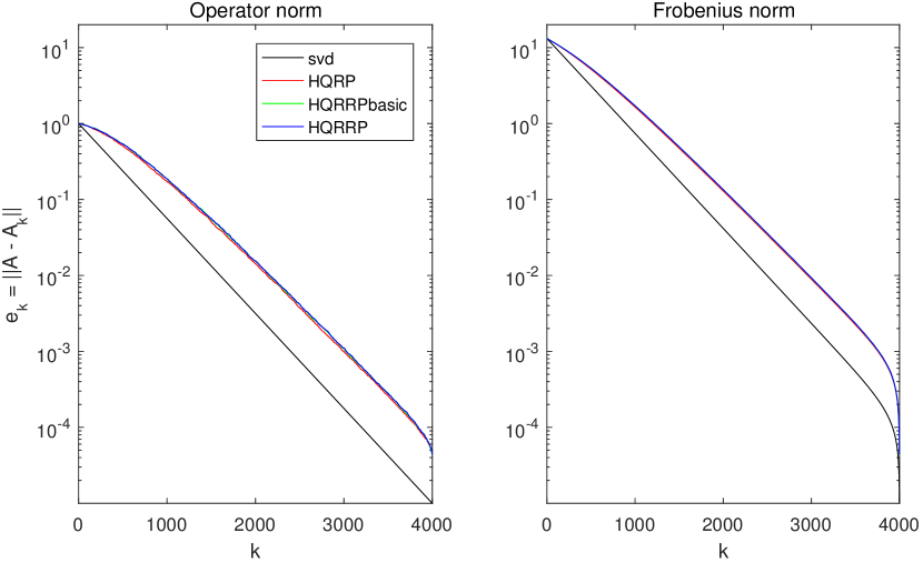
Fig. 6: Residual errors $e_{k}$ for “Matrix 1” as a function of the truncation rank $k$, cf. (15). The red line shows the results from traditional column pivoting, while the green and blue lines refer to the randomized methods we propose. The black line indicates the theoretically minimal errors resulting from a rank-$k$ partial singular value decomposition.

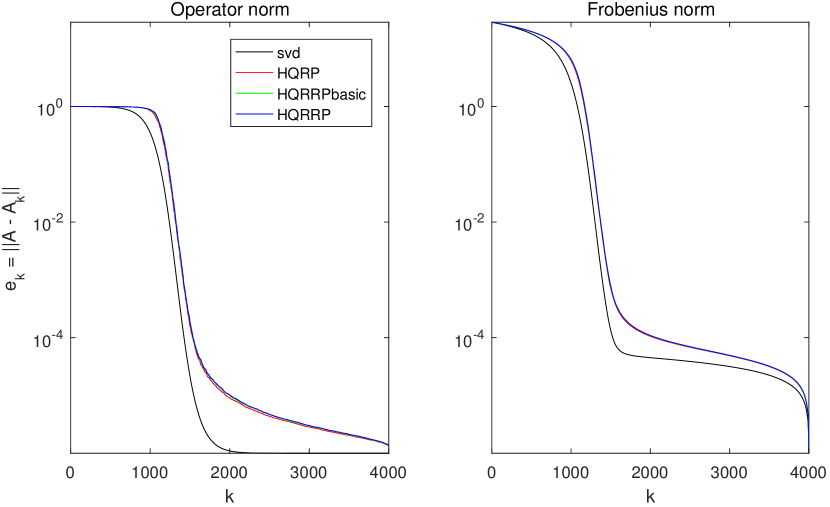
Fig. 7: Residual errors $e_{k}$ for “Matrix 2” as a function of the truncation rank $k$. Notation is the same as in Figure 6.

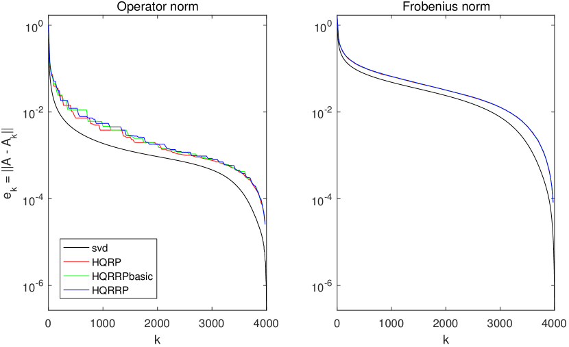
Fig. 8: Residual errors $e_{k}$ for “Matrix 3” (discretized boundary integral operator) as a function of the truncation rank $k$. Notation is the same as in Figure 6.

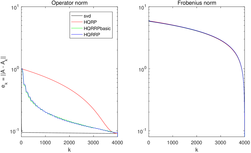
Fig. 9: Residual errors $e_{k}$ for “Matrix 4” (Kahan) as a function of the truncation rank $k$. Notation is the same as in Figure 6.

When classical column pivoting is used, the factorization (14) produced has the property that the diagonal entries of $R$ are strictly decaying in magnitude

$$|R(1,1)|\geq|R(2,2)|\geq|R(3,3)|\geq\cdots$$

When the randomized pivoting strategies are used, this property is not enforced. To illustrate this point, we show in Figure 10 the values of the diagonal entries obtained by the randomized strategies versus what is obtained with classical column pivoting.

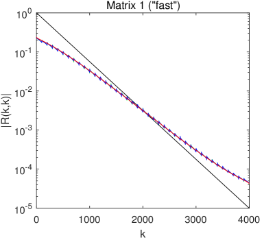
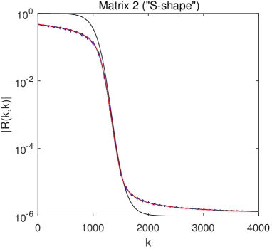
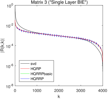
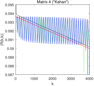
Fig. 10: For each of the four test matrices described in Section 4.2, we show the magnitudes of the diagonal entries in the “R”-factor in a column pivoted QR factorization. We compare classical column pivoting (red) with the two randomized techniques proposed here (blue and green). We also show the singular values of each matrix (black) for reference.

5 Conclusions and future work

We have described the algorithm HQRRP which is a blocked version of Householder QR with column pivoting. The main innovation compared to earlier work is that pivots are determined in groups using a technique based on randomized projections. We demonstrated that the quality of the chosen pivots is for practical purposes indistinguishable from traditional column pivoting (cf. Figures 6 – 8), and that the dominant term in the asymptotic flop count equals that of non-pivoted QR. Importantly, we also demonstrated through numerical experiments that HQRRP is very fast, in fact almost as fast as unpivoted HQR.

The technique described opens up several potential avenues for future research. The speed gains we demonstrate on single core and shared memory multicore machines is due to the reduction in data movement. Equivalently, data moved between memory layers is carefully amortized. We expect the technique described to have an even more pronounced advantage over traditional column pivoted QR when implemented in more severely communication constrained environments such as a matrix processed on a GPU or a distributed memory parallel machine, or stored out-of-core.

The randomized sampling techniques we describe can also be used to construct very close to optimal rank-revealing factorizations. To describe the idea, we note that a column pivoted QR factorization of a given matrix $A$ can be written as

$$A=Q\,R\,P^{*},$$ (16)

where $Q$ is orthonormal, $R$ is upper triangular, and $P$ is a permutation matrix. In this manuscript, we used randomized sampling to determine the permutation matrix $P$. It turns out that for a modest additional cost, one can build a factorization that takes the form (16), but with both $Q$ and $P$ built as products of Householder reflectors. This generalization allows us to bring $R$ not only to upper triangular form, but very close to being diagonal, with accurate approximations to the singular values of $A$ on its diagonal. This discovery was reported in [28], and is a subject of ongoing research.

How to scale the presented algorithm to very large numbers of cores is an open research question. Techniques such as “compute ahead” will have to be employed to ensure that the factorization of the current panel ($A_{11}$ and $A_{21}$) and downdate of $Y$ do not start dominating the parts of the computation that can be cast in terms of gemm.

6 Software

A number of implementations of the discussed algorithm are available under 3-clause (modified) BSD license from:

https://github.com/flame/hqrrp

Included are implementations that directly link to LAPACK [3] as well as implementations that use the libflame [30, 17] library. For those who use the LAPACK routine dgeqp3 routine, a plug compatible routine dgeqp4 is provided.

A distributed memory implementation of the algorithm has been incorporated into the Elemental software package by Jack Poulson et al [29], available at:

https://github.com/elemental/Elemental

Acknowledgments

The research reported was supported by DARPA, under the contract N66001-13-1-4050, and by the NSF, under the contracts DMS-1407340, DMS-1620472, and ACI-1148125/1340293. Any opinions, findings and conclusions or recommendations expressed in this material are those of the author(s) and do not necessarily reflect the views of the National Science Foundation (NSF).

References

- [1] Bradley K Alpert. Hybrid Gauss-trapezoidal quadrature rules. SIAM Journal on Scientific Computing, 20(5):1551–1584, 1999.
- [2] AMD. AMD Core Math Library. http://developer.amd.com/tools-and-sdks/cpu-development/amd-core-math-library-acml/.
- [3] E. Anderson, Z. Bai, C. Bischof, L. S. Blackford, J. Demmel, Jack J. Dongarra, J. Du Croz, S. Hammarling, A. Greenbaum, A. McKenney, and D. Sorensen. LAPACK Users’ guide (third ed.). SIAM, Philadelphia, PA, USA, 1999.
- [4] C. H. Bischof and Gregorio Quintana-Ortí. Algorithm 782: Codes for rank-revealing QR factorizations of dense matrices. ACM Trans. Math. Soft., 24(2):254–257, 1998.
- [5] C. H. Bischof and Gregorio Quintana-Ortí. Computing rank-revealing QR factorizations of dense matrices. ACM Trans. Math. Soft., 24(2):226–253, 1998.
- [6] Christian Bischof and Charles Van Loan. The WY representation for products of Householder matrices. SIAM J. Sci. Stat. Comput., 8(1):s2–s13, Jan. 1987.
- [7] Jack J. Dongarra, Jeremy Du Croz, Sven Hammarling, and Iain Duff. A set of level 3 basic linear algebra subprograms. ACM Trans. Math. Soft., 16(1):1–17, March 1990.
- [8] Jack J. Dongarra, Iain S. Duff, Danny C. Sorensen, and Henk A. van der Vorst. Solving Linear Systems on Vector and Shared Memory Computers. SIAM, Philadelphia, PA, 1991.
- [9] Petros Drineas, Ravi Kannan, and Michael W. Mahoney. Fast Monte Carlo algorithms for matrices. II. Computing a low-rank approximation to a matrix. SIAM J. Comput., 36(1):158–183 (electronic), 2006.
- [10] J. Duersch and M. Gu. True BLAS-3 performance QRCP using random sampling, 2015. arXiv preprint #1509.06820.
- [11] Carl Eckart and Gale Young. The approximation of one matrix by another of lower rank. Psychometrika, 1(3):211–218, 1936.
- [12] Alan Frieze, Ravi Kannan, and Santosh Vempala. Fast Monte-Carlo algorithms for finding low-rank approximations. J. ACM, 51(6):1025–1041 (electronic), 2004.
- [13] Gene H. Golub and Charles F. Van Loan. Matrix Computations. The Johns Hopkins University Press, Baltimore, 3nd edition, 1996.
- [14] Kazushige Goto and Robert A Geijn. Anatomy of high-performance matrix multiplication. ACM Transactions on Mathematical Software (TOMS), 34(3):12, 2008.
- [15] Kazushige Goto and Robert A. van de Geijn. On reducing TLB misses in matrix multiplication. Technical Report CS-TR-02-55, Department of Computer Sciences, The University of Texas at Austin, 2002.
- [16] Ming Gu and Stanley C. Eisenstat. Efficient algorithms for computing a strong rank-revealing QR factorization. SIAM J. Sci. Comput., 17(4):848–869, 1996.
-
[17]
John A. Gunnels, Fred G. Gustavson, Greg M. Henry, and Robert A. van de Geijn.
FLAME: Formal Linear Algebra Methods Environment.
ACM Trans. Math. Soft., 27(4):422–455, December 2001.
Download from http://www.cs.utexas.edu/users/flame/web/FLAMEPublications.htmlhttp://www.cs.utexas.edu/users/flame/web/FLAMEPublications.html. - [18] Nathan Halko, Per-Gunnar Martinsson, and Joel A. Tropp. Finding structure with randomness: Probabilistic algorithms for constructing approximate matrix decompositions. SIAM Review, 53(2):217–288, 2011.
- [19] IBM. Engineering and Scientific Subroutine Library. http://www-03.ibm.com/systems/power/software/essl/.
- [20] Intel. Math Kernel Library. http://developer.intel.com/software/products/mkl/.
- [21] Thierry Joffrain, Tze Meng Low, Enrique S. Quintana-Ortí, Robert van de Geijn, and Field G. Van Zee. Accumulating Householder transformations, revisited. ACM Trans. Math. Softw., 32(2):169–179, June 2006.
- [22] William Kahan. Numerical linear algebra. Canadian Math. Bull, 9(6):757–801, 1966.
- [23] Edo Liberty, Franco Woolfe, Per-Gunnar Martinsson, Vladimir Rokhlin, and Mark Tygert. Randomized algorithms for the low-rank approximation of matrices. Proc. Natl. Acad. Sci. USA, 104(51):20167–20172, 2007.
- [24] Michael W Mahoney. Randomized algorithms for matrices and data. Foundations and Trends® in Machine Learning, 3(2):123–224, 2011.
- [25] P.-G. Martinsson and S. Voronin. A randomized blocked algorithm for efficiently computing rank-revealing factorizations of matrices, mar 2015. ArXiv.org e-print #1503.07157. To appear in the SIAM Journal on Scientific Computing.
- [26] Per-Gunnar Martinsson, Vladimir Rokhlin, and Mark Tygert. A randomized algorithm for the approximation of matrices. Technical Report Yale CS research report YALEU/DCS/RR-1361, Yale University, Computer Science Department, 2006.
- [27] Per-Gunnar Martinsson, Vladimir Rokhlin, and Mark Tygert. A randomized algorithm for the decomposition of matrices. Appl. Comput. Harmon. Anal., 30(1):47–68, 2011.
- [28] P.G. Martinsson. Blocked rank-revealing qr factorizations: How randomized sampling can be used to avoid single-vector pivoting, 2015. arXiv preprint #1505.08115.
- [29] Jack Poulson, Bryan Marker, Robert A Van de Geijn, Jeff R Hammond, and Nichols A Romero. Elemental: A new framework for distributed memory dense matrix computations. ACM Transactions on Mathematical Software (TOMS), 39(2):13, 2013.
- [30] Enrique S. Quintana, Gregorio Quintana, Xiaobai Sun, and Robert van de Geijn. A note on parallel matrix inversion. SIAM J. Sci. Comput., 22(5):1762–1771, 2001.
- [31] Gregorio Quintana-Ortí, Xiaobai Sun, and Christian H. Bischof. A BLAS-3 version of the QR factorization with column pivoting. SIAM Journal on Scientific Computing, 19(5):1486–1494, 1998.
- [32] Robert Schreiber and Charles Van Loan. A storage-efficient WY representation for products of Householder transformations. SIAM J. Sci. Stat. Comput., 10(1):53–57, Jan. 1989.
- [33] G.W. Stewart. Matrix Algorithms Volume 1: Basic Decompositions. SIAM, 1998.
-
[34]
Field G. Van Zee.
libflame: The Complete Reference.
www.lulu.com, 2012.
Download from http://www.cs.utexas.edu/users/flame/web/FLAMEPublications.htmlhttp://www.cs.utexas.edu/users/flame/web/FLAMEPublications.html. - [35] Field G. Van Zee, Ernie Chan, Robert van de Geijn, Enrique S. Quintana-Ortí, and Gregorio Quintana-Ortí. The libflame library for dense matrix computations. IEEE Computation in Science & Engineering, 11(6):56–62, 2009.
- [36] Field G. Van Zee and Robert A. van de Geijn. BLIS: A framework for rapidly instantiating BLAS functionality. ACM Transactions on Mathematical Software, 41(3), 2015.
- [37] S. Voronin and P.G. Martinsson. A CUR factorization algorithm based on the interpolative decomposition. arXiv.org, 1412.8447, 2014.
- [38] David P Woodruff. Sketching as a tool for numerical linear algebra. arXiv preprint arXiv:1411.4357, 2014.
- [39] Xianyi Zhang, Qian Wang, and Yunquan Zhang. Model-driven level 3 BLAS performance optimization on loongson 3a processor. In Proceedings of the 2012 IEEE 18th International Conference on Parallel and Distributed Systems, pages 684–691. IEEE Computer Society, 2012.