Extending the MINLO method

Abstract

We consider improving Powheg+Minlo simulations, so as to also render them NLO accurate in the description of observables receiving contributions from events with lower parton multiplicity than present in their underlying NLO calculation. On a conceptual level we follow the strategy of the so-called Minlo^′ programs. Whereas the existing Minlo^′ framework requires explicit analytic input from higher order resummation, here we derive an effective numerical approximation to these ingredients, by imposing unitarity. This offers a way of extending the Minlo^′ method to more complex processes, complementary to the known route which uses explicit computations of high-accuracy resummation inputs. Specifically, we have focused on Higgs-plus-two-jet production (Hjj) and related processes. We also consider how one can cover three units of multiplicity at NLO accuracy, i.e. we consider how the Hjj-Minlo simulation may yield NLO accuracy for inclusive H, Hj and Hjj quantities. We perform a feasibility study assessing the potential of these ideas.

1 Introduction

In recent years, next-to-leading order parton shower (Nlops) matching techniques have been developed and realized as practical simulation tools, routinely used in LHC data analysis Frixione:2002ik ; Nason:2004rx ; Frixione:2007vw ; Alioli:2010xd ; Platzer:2011bc ; Hoeche:2011fd ; Alwall:2014hca . By now Nlops methods have been applied to many processes involving the production of a primary colourless system, e.g. a massive boson, $\mathcal{B}$, in association with jets ($\mathcal{B}n$j) Alioli:2010qp ; Frederix:2011ig ; Hoeche:2012ft ; Campbell:2012am ; Re:2012zi . A $\mathcal{B}n$j Nlops simulation yields NLO accuracy for $\mathcal{B}+n$-jet inclusive observables, and LO accuracy for $\mathcal{B}+m$-jet ones ($m=n+1$), while its predictions for more inclusive observables are divergent. Motivated by the success of leading order matrix element-parton shower multi-jet merging approaches in the earlier part of the last decade Mangano:2001xp ; Catani:2001cc ; Lonnblad:2001iq ; Mrenna:2003if , it has been considered highly desirable to combine Nlops generators for $\mathcal{B}n$j processes corresponding to different jet multiplicity, $n$, to obtain a unified simulation output, consistently describing inclusive $\mathcal{B}$, $\mathcal{B}+1$-jet ($\mathcal{B}$j) and $\mathcal{B}+2$-jet ($\mathcal{B}$jj) observables, simultaneously, with NLO accuracy.

This merging problem has been addressed by a number of groups in the last few years Lavesson:2008ah ; Alioli:2011nr ; Hoeche:2012yf ; Gehrmann:2012yg ; Frederix:2012ps ; Alioli:2012fc ; Platzer:2012bs . All of these approaches separate the output of each component simulation ($\mathcal{B}$, $\mathcal{B}$j or $\mathcal{B}$jj) according to the jet multiplicity of the events it produces, discarding those having a multiplicity for which the generator does not possess the relevant NLO corrections. Having processed the output of each simulation in this way, the event samples are joined to give an inclusive sample. Loosely speaking, each generator can be regarded as contributing a single exclusive jet bin to the final inclusive sample, the magnitude of each bin being predominantly determined by the jet resolution scale used in performing the merging, the so-called merging scale. Different approaches use different means to mitigate the dependence on this unphysical scale.

If the merging scale is too high one loses the benefits of the higher multiplicity generators, describing relatively hard jets with tree-level accuracy, or the parton-shower approximation. If the merging scale is too low, the inclusive sample is dominated by the higher-multiplicity generators, which in general leads to unitarity violation, whereby more inclusive quantities like the total inclusive cross section, exhibit spurious differences with respect to their corresponding conventional NLO predictions. The Geneva approach Alioli:2012fc can completely avoid unitarity violation, and even the introduction of a merging scale, by employing very high accuracy resummations. The method has been demonstrated for effectively merging two units of multiplicity (without a merging scale) in the context of an NNLL^′+NNLO parton shower matched simulation of the Drell-Yan process Alioli:2015toa . In the sense that it proposes to resolve the merging problem through implementing sufficiently high order resummation, Geneva represents the best solution of merging problem. However, details pertaining to exactly how this is done are subject to debate in the community. In the Unlops approach Lonnblad:2012ix unitarity is exactly maintained for sufficiently inclusive quantities, through what the authors refer to as ‘subtract-what-you-add’ approach. Nevertheless, the Unlops method is affected by other complications connected to the presence of a merging scale.

In the Minlo framework Hamilton:2012np , fully differential NLO cross sections for processes of type $\mathcal{B}+n-\mathrm{jets}$ are matched onto a leading log resummation of the exclusive $n-$jet cross section, as defined by the $k_{t}$-jet algorithm, with $\mathcal{B}$ here referring typically to a given collection of colourless final-state particles. This is the generalization, to the NLO level, of the resummation applied in the Ckkw formalism Catani:2001cc ; Krauss:2002up to the highest multiplicity tree level matrix element Mrenna:2003if . Essentially the $n$-hardest pseudopartons found by the $k_{t}$-jet algorithm have a distribution which is equivalent to that of a parton shower simulation of $\mathcal{B}$-production with, in addition, matching to the exact NLO $\mathcal{B}n$j matrix elements.

Whereas previously the leading order parts of these cross sections themselves would exhibit unphysical divergences when the Born partons became soft and/or collinear to one another, with the Minlo prescription applied their behavior is instead regular, physical and sensible, i.e. $\mathcal{B}n$j computations with the Minlo prescription also yield physical results for $\mathcal{B}m$j ($m<n$) and even fully inclusive $\mathcal{B}$-production observables. In the case of $\mathcal{B}$j, with $\mathcal{B}$ a W/Z/Higgs boson, it was found that the standard Minlo procedure yielded results for inclusive $\mathcal{B}$ production observables equivalent to conventional NLO ones up to terms $\mathcal{O}(\alpha_{{\scriptscriptstyle\mathrm{S}}}^{3/2})$ relative to the LO component Hamilton:2012rf . In the same article it was proven how, by delicate adjustment of the Minlo Sudakov form factor and clustering procedure, the spurious $\mathcal{O}(\alpha_{{\scriptscriptstyle\mathrm{S}}}^{3/2})$ terms could be eliminated, with the subsequent $\mathcal{B}$j-Minlo^′ calculations achieving NLO accuracy for both $\mathcal{B}$ and $\mathcal{B}$j inclusive observables; in the following we call the improved Minlo procedure of ref. Hamilton:2012rf Minlo^′ to distinguish it from the original Minlo prescription Hamilton:2012np . Thus one obtains, from the single NLO calculation of $\mathcal{B}$j production, also the fully differential NLO calculation of $\mathcal{B}$ production. The Minlo^′ calculation can then be matched to a parton shower using the standard techniques Frixione:2002ik ; Nason:2004rx ; Frixione:2007vw . When viewed in the context of the recent work in merging multiple NLO calculations together this amounts to merging without any unphysical merging scale. It was also demonstrated in refs. Hamilton:2013fea ; Karlberg:2014qua ; Astill:2016hpa how to promote the Minlo^′ simulations to Nnlops simulations.

While the modifications made in going from Minlo to Minlo^′ involve including higher order terms in the Sudakov form factor, and lead to the recovery of NLO accuracy also for inclusive $\mathcal{B}$ observables, the related resummation is not improved in accuracy. The resummation of the $\mathcal{B}$ system’s transverse momentum is $\mathrm{NNLL}_{\sigma}$ accurate Ellis:1997ii ; Frixione:1998dw before and after the inclusion of the latter terms in the Sudakov form factor Hamilton:2012rf (and before Nlops matching adds ambiguities). Thus, Minlo^′ amounts to the Minlo method with additional, subtle, unitarization. This is in difference to the Geneva approach, wherein higher order resummation is taken as the main defining specification, with unitarization coming ‘for free’ along with the latter Alioli:2012fc ; Alioli:2013hqa ; Alioli:2015toa . In this sense Minlo^′ is, minimally, the same as the Powheg method. Indeed, in the Powheg method a very specific Sudakov form factor is required to achieve an exact unitarization, needing terms in the exponent that are sub-leading with respect to the resummation accuracy to do so, including even power suppressed terms that are nothing to do with resummation.

To realize the Minlo^′ method one needs to know the $v\rightarrow 0$ singular part of the $\mathcal{B}$j cross section differential in the underlying Born variables, $\Phi_{{\scriptscriptstyle\mathcal{B}}}$, describing the kinematics of the produced $\mathcal{B}$-final state, where $v$ is a variable measuring radiation hardness, at NLO; this information may be obtained from suitably integrated NLO predictions for the spectrum, or from fixed order expansion of $\mathrm{N}^{3}\mathrm{LL}_{\sigma}$ resummation. In the case of ref. Hamilton:2012rf $v$ was given by the transverse momentum of the produced $W/Z/$Higgs boson, for which the latter NLO distributions have long been known in the literature Arnold:1990yk ; deFlorian:2001zd ; Glosser:2002gm . Recently these distributions have also become available to the same level of accuracy for the transverse momentum of the hardest produced jet Banfi:2012yh ; Becher:2012qa ; Tackmann:2012bt ; Banfi:2012jm ; Becher:2013xia ; Banfi:2013eda ; Banfi:2015pju , with which an equally accurate Minlo^′ calculation could have been developed. For more complicated observables, such as those which might be used for implementing the Minlo^′ method in the context of higher-multiplicity processes, with the exception of the $N$-jettiness variable Stewart:2009yx ; Stewart:2010qs ; Stewart:2010tn ; Berger:2010xi ; Jouttenus:2011wh ; Boughezal:2015dva ; Boughezal:2015aha ; Gaunt:2015pea , these distributions are (so far) not available in the literature. We note, however, that important progress is being made in the direction of automated approaches to final-state resummation at NNLL Banfi:2014sua , valid for broad classes of observables, including those we consider in the present work. Whenever these theoretical ingredients become available, the Minlo^′ method is in principle straightforward to apply, to make a NLO $\mathcal{B}n$j calculation simultaneously NLO accurate for $\mathcal{B}m$j ($m=n-1$) observables etc; many of the details for that are clarified by the present work.

Nevertheless, even when all the necessary theoretical ingredients are at hand, experience with the $\mathcal{B}$j-Minlo^′ calculations tells that the results of implementations are sometimes not as ideal as one might have liked. The Minlo^′ codes are proven to return conventional NLO results for inclusive $\mathcal{B}$ and $\mathcal{B}$j observables up to NNLO sized ambiguities and power corrections. In practice the Hj-Minlo^′ calculation was found to give very satisfactory agreement with the regular NLO predictions for inclusive Higgs boson production. On the other hand, comparing Wj-Minlo^′ and Zj-Minlo^′ predictions for inclusive W and Z production to those of regular NLO calculations, one can see numerical differences between the two sets of formally equivalent results, which don’t really sit easily with the fact that the two formally agree up to NNLO-sized ambiguities. In the Wj-Minlo^′ case, the inclusion of the relevant NNLL terms in the Sudakov form factor do not lead to noticeably better agreement with the conventional NLO cross sections than those obtained with the original Minlo prescription. We also point out that the true NNLO corrections to Higgs boson production are large, $\sim 20-30\%$, thus the almost perfect agreement of Hj-Minlo^′ with conventional NLO calculations for inclusive Higgs boson production — which looks to be a striking vindication of the theoretical framework — should be considered fortuitous.

Some people (like us) may be dismissive of numerical disagreement between $\mathcal{B}$j-Minlo^′ and standard NLO predictions for fully inclusive observables, since the Minlo^′ method has been rigorously proven. Others may be less comfortable accepting the fact that these differences arise from contributions beyond the formal accuracy of either type of calculation, given their size in some cases. If $5-6\%$ differences can be found in total inclusive cross sections for inclusive W and Z production, it does not seem unreasonable to expect that larger differences may be found in more complex processes, with more powers of the strong coupling associated to the LO contribution and a richer kinematic content. Assuming one is content to dismiss differences due to higher order ambiguities, for complex processes, with even more complex calculations underlying them, it will be difficult to satisfy oneself that the level of numerical disagreement is of this kind.

A final motivation for considering to extend the reach of the Minlo^′ method is that of merging NLO calculations differing by more than one unit of jet multiplicity. Specifically, one would ultimately like a Minlo^′ procedure applied to $\mathcal{B}$jj-Minlo such that it retrieves NLO accuracy for inclusive $\mathcal{B}$, $\mathcal{B}$j and $\mathcal{B}$jj observables. Naive extension of the Minlo^′ method then implies having a $\mathrm{N}^{3}\mathrm{LL}_{\sigma}$-accurate nested resummation with which to base it on. While the resummation community is making impressive progress in recent years Pietrulewicz:2016nwo , the prospects for obtaining the high-accuracy ingredients needed to tackle this issue in the near future are unclear to us.

Noting these desirable and undesirable features of the existing Minlo^′ method, we investigated extending it in a number of ways:

1. The Minlo^′ specification can be reached with only limited knowledge of the required Sudakov form factors (at least $\mathrm{NLL}_{\sigma}$).

   Thus, one can begin to make Minlo^′ simulations for more complex processes.

2. $\mathcal{B}$jj/$\mathcal{B}$j-Minlo^′ predictions for $\mathcal{B}$j/inclusive $\mathcal{B}$ observables agree precisely with those of the corresponding conventional NLO calculations.

   Numerical ambiguities between conventional inclusive NLO predictions and the associated Minlo^′ ones can be largely eliminated.

3. NLO $\mathcal{B}$jj calculations can yield simultaneously NLO predictions for $\mathcal{B}$j and inclusive $\mathcal{B}$ production observables.

   The method to produce Nnlops simulations of $\mathcal{B}$ production can follow exactly as in ref. Hamilton:2013fea .

In the present work we suggest an alternative approach to Minlo^′, meeting the objectives listed overhead, and we present a feasibility study confirming its potential. The basic concept is very close to that of the original Minlo^′ method and, more broadly speaking, the Powheg approach itself. As with the original Minlo^′ formulation, we attribute discrepancies of $\mathcal{B}m$j-Minlo predictions for $\mathcal{B}n$j ($m=n+1$) inclusive quantities, with respect to conventional fixed order results, as owing to deficiencies in the Sudakov form factor employed in the former. In the existing Minlo^′ framework, the correction to the Sudakov form factor which leads to the elimination of these discrepancies, is derived from highly intricate, third-party, analytic computations, of the NLO $\mathcal{B}m$j radiation spectrum. Here, instead, we determine the relation between $\mathcal{B}m$j-Minlo predictions for $\mathcal{B}n$j Born kinematics and those of conventional (N)NLO, in terms of the a priori unknown correction factor to the $\mathcal{B}m$j-Minlo Sudakov form factor. Since both the $\mathcal{B}m$j-Minlo and conventional fixed order predictions for the Born kinematics are to-hand, we can then solve this relation for the unknown Sudakov correction, numerically, to sufficent accuracy, bringing the $\mathcal{B}n$j Born kinematics of $\mathcal{B}m$j-Minlo into complete agreement with regular (N)NLO predictions. This then renders $\mathcal{B}m$j-Minlo (N)NLO accurate for $\mathcal{B}n$j inclusive observables, while maintaining NLO accuracy for $\mathcal{B}m$j ones. We arrive at the aforesaid defining equation for our method by manipulating the original Minlo^′ computation, neglecting terms which lead to irrelevant higher order ambiguities (sects. 2.4-2.6). With such an approach the Minlo^′ and Nnlops methods become much more easily/widely applicable than before, being no longer contingent on the existence of high accuracy, observable- and process-dependent analytic ingredients. To implement this approach it is sufficient to have only $\mathrm{NLL}_{\sigma}$ accuracy in the initial, uncorrected, Minlo simulation and an NLO (or NNLO) prediction for the Born kinematics of the associated lower multiplicity process. At the same time, residual ambiguities between Minlo^′ predictions and conventional NLO/Nlops are brought under much tighter control, and can be completely removed, if so desired.

We do not propose to replace the existing Minlo^′ method, but rather to supplement it and, as such, we don’t question the importance of efforts to provide further resummation input which that fundamentally needs — on the contrary, it’s clear that work is, at the very least, complementary to the improvements discussed here. The study of the problem of combining multiple NLO simulations together is not long started though, so we consider more options, understanding and investigations in this direction, to be still welcome.

In section 2 we discuss the Minlo procedure and its extension(s), in the context of recovering NLO accuracy for $\mathcal{B}m\textsc{j}$ processes from NLO $\mathcal{B}n\textsc{j}$ calculations, $m=n-1$, without any merging scale, focusing on $\mathcal{B}\textsc{j}$ and $\mathcal{B}\textsc{jj}$. We derive $\mathrm{NNLL}_{\sigma}$ resummation formulas from the Caesar formalism Banfi:2004yd and compare these to the equivalent Minlo/Ckkw results. This reveals conventional ways in which to improve the $\mathcal{B}$jj-Minlo procedure, in particular it gives details for improving the accuracy of the Sudakov form factor to $\mathrm{NNLL}_{\sigma}$; we leave the implementation of such improvements for future work. With the true resummation clarified at $\mathrm{NNLL}_{\sigma}$, by the latter comparison to Caesar, we proceed with clarity to propose how one could infer an effective approximation to higher order Sudakov terms, needed by Minlo^′, by imposing unitarity. In section 3 we propose that the latter method can also be used for the purposes of rendering $\mathcal{B}\textsc{jj}$ Minlo simulations simultaneously NLO accurate in the description of inclusive $\mathcal{B}$ and $\mathcal{B}\textsc{j}$ production. Section 4 presents a feasibility study assessing the potential of these ideas. We summarize our findings and conclude in sect. 5.

2 Merging two units of multiplicity

In the following we ultimately present a method for merging Nlops simulations of $\mathcal{B}$- and $\mathcal{B}$j-production and, separately, $\mathcal{B}$j- and $\mathcal{B}$jj-production without any actual merging. More precisely, the improved Minlo procedure will render the $\mathcal{B}$j simulation also NLO accurate for $\mathcal{B}$-production and, in the case of $\mathcal{B}$jj it will build in NLO precision for $\mathcal{B}$j.

We remind that in this work we refer to the leading tower of logarithms in the spectrum, terms $\mathcal{O}(\bar{\alpha}_{{\scriptscriptstyle\mathrm{S}}}^{n}L^{2n-1})$, as $\mathrm{LL}_{\sigma}$, with $\mathrm{NLL}_{\sigma}$ denoting the next-to-leading log tower, $\mathcal{O}(\bar{\alpha}_{{\scriptscriptstyle\mathrm{S}}}^{n}L^{2n-2})$, $\mathrm{NNLL}_{\sigma}$ for the next-to-next-to-leading log tower $\mathcal{O}(\bar{\alpha}_{{\scriptscriptstyle\mathrm{S}}}^{n}L^{2n-3})$, and so forth.

In section 2.1 we introduce preliminary notation and definitions, in particular regarding the clustering variables which the Minlo procedure is to resum, and the so-called underlying Born kinematics that the resummation is performed about. In section 2.2 we present a formula for $\mathrm{NNLL}_{\sigma}$ resummation of these clustering variables ($k_{t}$-jet resolutions) based on the Caesar resummation framework Banfi:2004yd . The Sudakov form factors of the latter are compared to the corresponding Minlo formulae in section 2.3. In section 2.4 we derive the fixed order expansion of the $\mathrm{NNLL}_{\sigma}$ Caesar formula and from this we show how our Minlo procedure applied to the $\mathcal{B}$j(j) NLO computations returns a matched, resummed, NLO accurate jet resolution spectrum. In doing so, we also assume that spurious, unknown, $\mathrm{NNLL}_{\sigma}$ or $\mathrm{N^{3}LL}_{\sigma}$ terms may arise in the Minlo resummation, owing to a lack of understanding of the true $\mathrm{N}^{3}\mathrm{LL}_{\sigma}$ spectrum truncated at NLO, and we closely monitor how these propagate through the Minlo procedure, to better understand and eradicate them, as needed. In section 2.5 we integrate over the Minlo jet resolution spectrum, determining that the distribution of the Born kinematics differs from that of conventional NLO owing to the latter spurious terms, which we have tracked and quarantined. In section 2.6 we first demonstrate how the original Minlo^′ approach removes such terms, by explicitly correcting the Minlo Sudakov form factor, leading to NLO accurate Born kinematics. In the second part of section 2.6, we present our new proposal. Over-simplifying somewhat, this amounts to using the constraint that the corrected Minlo predictions must recover NLO (or NNLO) results for the inclusive Born kinematics, as a defining equation for the elusive Sudakov correction factors, needed to promote Minlo to Minlo^′. This equation can no doubt be solved for the latter in several ways, and we present one basic, simple, way to do so. In order to maintain NLO accuracy in the higher multiplicity phase space, it is necessary that the initial Minlo resummation be at least $\mathrm{NLL}_{\sigma}$ accurate, however, this is an easily obtainable threshold by today’s standards.

We underline now that it is a working assumption of the Caesar framework, that the underlying Born kinematics, about which the resummation of soft radiation is carried out, are not themselves associated with large logarithmic corrections, i.e. it is assumed that the radiating particles in the hard underlying Born kinematics are well separated. For the case of $\mathcal{B}$ production, with only two radiating particles in the initial-state, the latter criterion is fulfilled automatically. On the other hand, for $\mathcal{B}$j production it implies that we have to restrict ourselves to a regime in which the final-state (pseudo-)parton in the underlying Born has transverse momentum of order the mass of $\mathcal{B}$, or greater. In other words, in this section 2 it should be understood that the $y_{12}$ resummation in $\mathcal{B}$j-production assumes $y_{01}\gtrsim\mathcal{O}(m_{{\scriptscriptstyle\mathcal{B}}}^{2})$. Only in section 3 will we consider extending down into the region where the transverse momentum of the final-state Born (pseudo-)parton is small.

2.1 Definitions: jet resolutions and underlying Born kinematics

Since it is underlies the whole discussion we first quickly present a reminder of the exclusive $k_{t}$-jet clustering procedure (for brevity we henceforth refer to pseudopartons obtained in the clustering sequence as just partons):

1. In an $n$-parton final-state we determine the smallest distance

   $$d^{\left(n\right)}=\mathrm{min}\left(\left\{d_{ij}\right\},\left\{d_{iB}\right\}\right)\,,$$

   where $\left\{d_{ij}\right\}$ is the set of measures

   $$d_{ij}=\mathrm{min}(k_{t,i}^{2},k_{t,j}^{2})\,(\left(\mathrm{y}_{i}-\mathrm{y}_{j}\right)^{2}+\left(\phi_{i}-\phi_{j}\right)^{2})/R^{2}\,,$$

   obtained by considering all pairwise combinations of final-state partons $i$ and $j$, with $k_{t,i}$, $\mathrm{y}_{i}$ and $\phi_{i}$ being, respectively, the transverse momentum, rapidity and azimuth of parton $i$, and $\{d_{iB}\}$ the set of all final-state transverse momenta:

   $$d_{iB}=k_{t,i}\,.$$

   $R$ is the so-called jet radius parameter which we take equal to be $1$.

2. If $d^{\left(n\right)}=d_{ij}$ partons $i$ and $j$ are replaced in the event by a single mother parton with four momentum $p_{i}+p_{j}$, otherwise, if $d^{\left(n\right)}=d_{i}$, particle $i$ is considered to have been similarly absorbed in one of the beam jets and is deleted from the event.

3. If further partons remain return to step 1, otherwise the clustering sequence terminates.

In order to have the $\mathcal{B}$j-Minlo calculation return NLO accuracy for inclusive $\mathcal{B}$ production and $\mathcal{B}$jj-Minlo likewise reproduce NLO accuracy for $\mathcal{B}$j quantities, we are interested to resum the $k_{t}$-jet resolution variables $y_{01}$ and $y_{12}$, which we here define as

$$y_{01}=\max_{n\geq 1}\{d^{\left(n\right)}\}\,, v_{01}=y_{01}/Q_{{\scriptscriptstyle\mathcal{B}\mathrm{\phantom{J}}}}^{2}\,,$$

$$y_{12}=\max_{n\geq 2}\{d^{\left(n\right)}\}\,, v_{12}=y_{12}/Q_{{\scriptscriptstyle\mathcal{B}\mathrm{J}}}^{2}\,,$$

where $Q_{{\scriptscriptstyle\mathcal{B}}}$ and $Q_{{\scriptscriptstyle\mathcal{B}\mathrm{J}}}$ are, in the context of the Caesar resummation framework Banfi:2004yd , the hard scales of the problem, largely determined by the respective Born kinematics. We take $Q_{{\scriptscriptstyle\mathcal{B}}}^{2}=m_{{\scriptscriptstyle\mathcal{B}}}^{2}$, where $m_{{\scriptscriptstyle\mathcal{B}}}$ is the invariant mass of the system $\mathcal{B}$, and $Q_{{\scriptscriptstyle\mathcal{B}\mathrm{J}}}^{2}=Q_{{\scriptscriptstyle\mathcal{B}}}^{2}v_{01}=y_{01}$. With this definition the resummation of $y_{12}$ amounts to — up to corrections owing to the lack of monotonicity of the clustering sequence in $d^{\left(n\right)}$, which we neglect — a resummation of large logarithms of the transverse momentum of the second hardest relative to the hardest branching in the event. For what follows we notate these large logarithms

$$L_{01}=\log\frac{1}{v_{01}},\quad\quad L_{12}=\log\frac{1}{v_{12}}\,.$$

In discussions and formulae that apply equally well to the $\mathcal{B}$j-Minlo and $\mathcal{B}$jj-Minlo computations we simply use $L$ to refer to either $L_{01}$ or $L_{12}$. Equally, we will use $y$ to ambiguously mean $y_{01}$ and $y_{12}$, and $v$ to mean $v_{01}$ and $v_{12}$, when safe to do so.

We now introduce the kinematic variables specifying the hard configurations about which we intend Minlo to resum the $y_{01}$ and $y_{12}$ variables. First consider applying the $k_{t}$-jet algorithm to events such that they are clustered to the point of containing just a single jet (pseudoparton) and the system/particle $\mathcal{B}$. We define directly from such ensembles $\mathcal{B}$j underlying Born variables, $\Phi_{{\scriptscriptstyle\mathcal{B}\mathrm{J}}}=\{\hat{\Phi}_{{\scriptscriptstyle\mathcal{B}}},\mathrm{y}_{{\scriptscriptstyle\mathcal{B}}},\mathrm{y}_{{\scriptscriptstyle\mathrm{J}}},p_{{\scriptscriptstyle\mathrm{T}}}^{{\scriptscriptstyle\mathrm{J}}},\phi_{{\scriptscriptstyle\mathrm{J}}}\}$, where the set $\hat{\Phi}_{{\scriptscriptstyle\mathcal{B}}}$ specifies the configuration of $\mathcal{B}$ in its rest frame, including its invariant mass, $\mathrm{y}_{{\scriptscriptstyle\mathrm{J}}}$ is the rapidity of the jet, $\mathrm{y}_{{\scriptscriptstyle\mathcal{B}}}$ is the rapidity of $\mathcal{B}$, $p_{{\scriptscriptstyle\mathrm{T}}}^{{\scriptscriptstyle\mathrm{J}}}$ the transverse momentum of the jet, and $\phi_{{\scriptscriptstyle\mathrm{J}}}$ its azimuthal angle. After a subsequent clustering with the $k_{t}$-jet algorithm the jet/pseudoparton is also removed leaving just the system $\mathcal{B}$, for which we further define $\mathcal{B}$ underlying Born variables $\Phi_{{\scriptscriptstyle\mathcal{B}}}=\{\hat{\Phi}_{{\scriptscriptstyle\mathcal{B}}},\mathrm{y}_{{\scriptscriptstyle\mathcal{B}}}\}$. Thus we can also write $\Phi_{{\scriptscriptstyle\mathcal{B}\mathrm{J}}}=\{\Phi_{{\scriptscriptstyle\mathcal{B}}},\mathrm{y}_{{\scriptscriptstyle\mathrm{J}}},p_{{\scriptscriptstyle\mathrm{T}}}^{{\scriptscriptstyle\mathrm{J}}},\phi_{{\scriptscriptstyle\mathrm{J}}}\}$.

The definitions of $\Phi_{{\scriptscriptstyle\mathcal{B}\mathrm{J}}}$ and $\Phi_{{\scriptscriptstyle\mathcal{B}}}$ can also be considered as projections from real (or multiple emission) kinematics onto Born kinematics for $\mathcal{B}$j and $\mathcal{B}$ final-states respectively; note that, strictly speaking, in that context the jet in the projected $\mathcal{B}$j kinematics should be understood as being massless. The choices of $\mathrm{y}_{{\scriptscriptstyle\mathcal{B}}}$ and $\mathrm{y}_{{\scriptscriptstyle\mathrm{J}}}$ are motivated by our expectation that even basic formulations of the $\mathcal{B}$j- and $\mathcal{B}$jj-Minlo^′ calculations will reproduce well the shapes of these quantities, as they are predicted in the respective (conventional) NLO $\mathcal{B}$ and $\mathcal{B}$j computations. Our choosing of $p_{{\scriptscriptstyle\mathrm{T}}}^{{\scriptscriptstyle\mathrm{J}}}$ in $\Phi_{{\scriptscriptstyle\mathcal{B}\mathrm{J}}}$ is made in light of the fact that this variable, as defined here, is equal to $\sqrt{y_{01}}$, which we expect to greatly increase the consistency between the $\mathcal{B}$j-Minlo^′ (which resums precisely $v_{01}$) and the $\mathcal{B}$jj-Minlo^′ calculations, which we intend to have identically reproduce NLO $\mathcal{B}$j predictions such as $p_{{\scriptscriptstyle\mathrm{T}}}^{{\scriptscriptstyle\mathrm{J}}}$, as defined here, according to the exclusive $k_{t}$-jet clustering algorithm. The latter consideration is important in the context of nesting the $v_{01}$ and $v_{12}$ resummations, with a view to having a $\mathcal{B}$jj-Minlo^′ simulation NLO accurate for $\mathcal{B}$jj, $\mathcal{B}$j, and inclusive $\mathcal{B}$ production processes.

2.2 $\mathrm{NNLL}_{\sigma}$ resummation

By differentiating and expanding the master resummation formula in ref. Banfi:2004yd , we are able to derive simultaneously $\mathrm{LL}$ and $\mathrm{NNLL}_{\sigma}$ accurate expressions for the $v_{01}$ and $v_{12}$ spectra in $\mathcal{B}$ and $\mathcal{B}$j production processes respectively. In a nutshell, one takes the $\mathrm{NLL}$ resummation of ref. Banfi:2004yd , matched to NLO, and proceeds to omit NLL terms $\mathcal{O}(\bar{\alpha}_{{\scriptscriptstyle\mathrm{S}}}^{3})$ and beyond in the resummed exponent, specifically those due to observable-dependent multiple emission effects. Details on these manipulations can be found in appendix A.1. The general expression we derive can be written simply in the form Dokshitzer:1978hw :

$$\frac{d\sigma_{{\scriptscriptstyle\mathcal{R}}}}{d\Phi dL} = \frac{d\sigma_{0}}{d\Phi}\,\left[1+\bar{\alpha}_{{\scriptscriptstyle\mathrm{S}}}\left(\mu_{{\scriptscriptstyle R}}^{2}\right)\,\mathcal{H}_{1}\left(\mu_{{\scriptscriptstyle R}}^{2}\right)\right]\,\frac{d}{dL}\,\left[\exp\left[\,-R\left(v\right)\,\right]\,\mathcal{L}\left(\left\{x_{\ell}\right\},\mu_{{\scriptscriptstyle F}},v\right)\right]\,,$$ (1)

where $\mathcal{L}$ is our luminosity factor

$$\mathcal{L}\left(\left\{x_{\ell}\right\},\mu_{{\scriptscriptstyle F}},v\right) = \prod_{\ell=1}^{n_{i}}\frac{q^{\left(\ell\right)}\left(x_{\ell},\mu_{{\scriptscriptstyle F}}^{2}v\right)}{q^{\left(\ell\right)}\left(x_{\ell},\mu_{{\scriptscriptstyle F}}^{2}\right)}\left[1+\sum_{\ell=1}^{n_{i}}\,\bar{\alpha}_{{\scriptscriptstyle\mathrm{S}}}\left(\mu_{{\scriptscriptstyle R}}^{2}v\right)\,\frac{\left[\boldsymbol{\mathcal{C}}_{1}\otimes\boldsymbol{\mathrm{q}}^{\left(\ell\right)}\right]_{i}\left(x_{\ell},\mu_{{\scriptscriptstyle F}}^{2}v\right)}{q^{\left(\ell\right)}\left(x_{\ell},\mu_{{\scriptscriptstyle F}}^{2}v\right)}\right]\,.$$ (2)

Since this form applies to both jet resolutions in $\mathcal{B}$ and $\mathcal{B}$j production, the components inside it should be understood as referring to one of these two processes, e.g. $\Phi$ and $L$ refer to $\Phi_{{\scriptscriptstyle\mathcal{B}\mathrm{J}}}$ and $L_{\text{12}}$ in the $\mathcal{B}$j case, and $\Phi_{{\scriptscriptstyle\mathcal{B}}}$ and $L_{01}$ in $\mathcal{B}$-production. Equally, $v$ refers to $v_{01}$ in the latter case and $v_{12}$ in the former.

First let’s overview the resummation formula, eq. 1, before disappearing into the details. The first factor in eq. 1, $d\sigma_{0}/d\Phi$, denotes the leading order cross section for $\mathcal{B}$ or $\mathcal{B}$j processes as appropriate. Within $d\sigma_{0}/d\Phi$ the scale used for the evaluation of the parton distribution functions is $\mu_{{\scriptscriptstyle F}}$ and the scale in any implicit strong coupling constant factors is $\mu_{{\scriptscriptstyle R}}$. The function $\mathcal{H}_{1}$ includes hard virtual corrections to $d\sigma_{0}/d\Phi$. The Sudakov form factor is present in eq. 1 as $\exp\left[-R\left(v\right)\right]$; here we have made a simplification with respect to the notation of ref. Banfi:2004yd , including in its definition contributions from soft-wide angle radiation and observable-dependent multiple emission corrections. The $q^{\left(\ell\right)}\left(x_{\ell},\mu^{2}\right)$ terms in the luminosity factor, eq. 2, are parton distribution functions (PDFs), for a given incoming leg, $\ell$, with momentum fraction $x_{\ell}$, evaluated at scale $\mu$. The product of PDF ratios runs over $n_{i}=2$ incoming legs. The functions $\mathcal{C}_{1}$ involved in convolutions with PDFs in the luminosity factor, $\mathcal{L}$, are due to universal hard-collinear corrections. The renormalization and factorization scales $\mu_{{\scriptscriptstyle R}}$ and $\mu_{{\scriptscriptstyle F}}$ are understood as being $\sim Q$ Banfi:2004yd .

To try to lighten the formulae we use the following abbreviations,

$$\bar{\alpha}_{{\scriptscriptstyle\mathrm{S}}}=\frac{\alpha_{{\scriptscriptstyle\mathrm{S}}}}{2\pi}\,,\quad\beta_{0}=\frac{11C_{A}-2n_{f}}{12\pi}\,,\quad\bar{\beta}_{0}=2\pi\beta_{0}\,.$$ (3)

The Sudakov form factor exponent in the $\mathrm{NNLL}_{\sigma}$ differential cross section formula (eq. 1) is given by

$$-R\left(v\right)=\int_{0}^{L}dL^{\prime}\,\left[\bar{\alpha}_{{\scriptscriptstyle\mathrm{S}}}\left(y^{\prime}\right)\,\left[2G_{12}\,L^{\prime}+G_{11}+2S_{1}\right]+\bar{\alpha}_{{\scriptscriptstyle\mathrm{S}}}^{2}\left(y^{\prime}\right)\,2G_{12}\,\left[K+4\mathcal{F}_{2}G_{12}\right]\,L^{\prime}\right]\,.$$ (4)

The $G_{ij}$ contributions are due to independent soft-collinear / collinear emission contributions, they are given by

$$\begin{array}[]{lll}G_{12}=-\frac{1}{2}\,\sum_{\ell}\,C_{\ell}\,,&&G_{11}=-2\,\sum_{\ell}\,B_{\ell}C_{\ell}\,,\end{array}$$ (5)

where

$$\left.\begin{array}[]{l}C_{\ell}=C_{F}\\ B_{\ell}=-\frac{3}{4}\end{array}\right\}\,\mbox{ for a quark leg}\,,\quad\quad\left.\begin{array}[]{l}C_{\ell}=C_{A}\\ B_{\ell}=-\frac{\bar{\beta}_{0}}{2C_{A}}\end{array}\right\}\,\mbox{ for a gluon leg}.$$ (6)

The sum, $\sum_{\ell}$, runs over all $n$ hard colour-charged legs $\ell$ — $n=2$ for $\mathcal{B}$-production, $n=3$ for $\mathcal{B}$j. Single logarithmic soft-wide angle emission contributions are included via the $S_{1}$ term. Soft-wide angle radiation is obviously sensitive to the structure of the underlying hard event on large angular scales, so in contrast to the collinear contributions above, this piece is sensitive to the orientation of the hard external legs and not just their charges. For $\mathcal{B}$ ($n=2$) and $\mathcal{B}$j($n=3$) processes we have

$$n=2:\quad S_{1} = -\left(C_{q}+C_{q^{\prime}}\right)\ln\frac{Q_{qq^{\prime}}}{Q_{{\scriptscriptstyle\mathcal{B}}}}\,,\quad$$ (7)

$$n=3:\quad S_{1} = -\frac{1}{2}\left(C_{q}+C_{q^{\prime}}\right)\ln\frac{Q_{{\scriptscriptstyle\mathcal{B}}}^{2}}{y_{01}}+\frac{1}{2}\left(C_{q}+C_{q^{\prime}}\right)\ln\frac{m_{{\scriptscriptstyle\mathcal{B}}}^{2}}{Q_{qq^{\prime}}^{2}}-\frac{1}{2}C_{g}\ln\frac{Q_{qg}^{2}Q_{q^{\prime}g}^{2}}{Q_{qq^{\prime}}^{2}y_{01}}$$

$$-\frac{1}{2}\left(C_{q}+C_{q^{\prime}}\right)\ln\frac{m_{{\scriptscriptstyle\mathcal{B}}}^{2}}{Q_{{\scriptscriptstyle\mathcal{B}}}^{2}}-\frac{1}{2}\sum_{\ell}\,C_{\ell}\ln\frac{y_{01}}{Q_{{\scriptscriptstyle\mathcal{B}\mathrm{J}}}^{2}}\,.$$

where $Q_{ij}=\sqrt{\left|2p_{i}.p_{j}\right|}$. For the case of two/three hard gluon legs, we simply replace $C_{F}$ by $C_{A}$ in $S_{1}$ and, in addition, $q$, $q^{\prime}$, $g$ with $g_{1}$, $g_{2}$, $g_{3}$ (see bottom of pg. 38 in ref. Banfi:2004yd ). By writing $S_{1}$ in this form for the $n=3$ case one can already glimpse, in the first term, its interpretation in terms of coherent emission from the $n=2$ kinematic underlying the $n=3$ one; we discuss this in more depth later on.

The $K$ in the $\mathcal{O}\left(\bar{\alpha}_{{\scriptscriptstyle\mathrm{S}}}^{2}\right)$ part of $R$ is the two-loop cusp anomalous dimension

$$K=C_{A}\left(\frac{67}{18}-\frac{\pi^{2}}{6}\right)-\frac{5}{9}n_{f}.$$ (9)

Concerning the Sudakov form factor, the only remaining part needing introduction is $\mathcal{F}_{2}$. The $\mathcal{F}\left(R^{\prime}\right)$ function of ref. Banfi:2004yd accounts for NLL corrections arising from a resummed observable’s sensitivity to multiple emission effects; for observables whose behavior is largely dictated by the leading single emission $\mathcal{F}\left(R^{\prime}\right)\rightarrow 1$. The Caesar $\mathcal{F}\left(R^{\prime}\right)$ factor is understood to depend only on the flavours of the particles entering and exiting the hard scattering and the multiple emission properties of the observable, it does not depend on the kinematics of the underlying hard scattering $\left(\Phi\right)$ Banfi:2004nk . To $\mathrm{NLL}$/$\mathrm{NNLL}_{\sigma}$ accuracy $\mathcal{F}\left(R^{\prime}\right)=1$ for the $v_{01}$ resummation ($\mathcal{B}$-production). The combination of factors $\mathcal{F}_{2}\left(2G_{12}\right)^{2}\,\bar{\alpha}_{{\scriptscriptstyle\mathrm{S}}}^{2}L^{2}$ is the next-to-leading term in the fixed order expansion of the $\mathcal{F}\left(R^{\prime}\right)$ function and as such defines $\mathcal{F}_{2}$. From refs. Banfi:2004nk ; Banfi:2001bz ; Banfi:2012yh we derive the following process-independent expression for $\mathcal{F}_{2}$, for jet rates in the exclusive $k_{t}$ algorithm

$$\mathcal{F}_{2}=-\frac{\pi^{2}}{16}\,\frac{\sum_{\ell=1}^{n}C_{\ell}^{2}-\sum_{\ell=1}^{n_{i}}C_{\ell}^{2}}{\left(\sum_{\ell=1}^{n}C_{\ell}\right)^{2}}\,,$$ (10)

We have tested this expression using the numerical implementation of the Caesar formalism for resummation of $y_{23}$ in hadronic jet production and $y_{12}$ in hadronic $Z$ boson production. With the exception of the $qg$ and $gq$ channels in $Z$ production, for which only 3% differences were found, our $\mathcal{F}_{2}$ expression yielded agreement with the Caesar program at the per mille level in all tested processes and channels.

In the resummation formula, eqs. 2-1, for the PDF dependent pieces we have adopted the notation

$$\boldsymbol{\mathrm{q}}\left(x,\mu_{{\scriptscriptstyle F}}^{2}\right)=\left(\begin{array}[]{c}q_{u}\left(x,\mu_{{\scriptscriptstyle F}}^{2}\right)\\ q_{\bar{u}}\left(x,\mu_{{\scriptscriptstyle F}}^{2}\right)\\ \vdots\\ g\left(x,\mu_{{\scriptscriptstyle F}}^{2}\right)\end{array}\right)\,,\quad\boldsymbol{\mathrm{P}}\left(x\right)=\left(\begin{array}[]{cccc}P_{qq}^{\left(0\right)}\left(x\right)&0&\cdots&P_{qg}^{\left(0\right)}\left(x\right)\\ 0&P_{qq}^{\left(0\right)}\left(x\right)\\ \vdots&&\ddots\\ P_{gq}^{\left(0\right)}\left(x\right)&&&P_{gg}^{\left(0\right)}\left(x\right)\end{array}\right)\,,$$ (11)

where $P_{ij}^{\left(0\right)}\left(x\right)$ are the regularized leading order Altarelli-Parisi splitting functions (see e.g. appendix A.3 of ref. Banfi:2004yd ). We also identify $q^{\left(\ell\right)}\left(x_{\ell},\mu^{2}\right)=\boldsymbol{\mathrm{q}}_{i}^{\left(\ell\right)}\left(x_{\ell},\mu^{2}\right)$, with $i$ the flavour of the hard parton with momentum $p_{\ell}$, and we employ the following notation to denote matrix multiplication and convolution in $x$-space

$$\left[\,\mathrm{\boldsymbol{\mathrm{P}}}\otimes\boldsymbol{\mathrm{q}}\,\right]_{i}\left(x,\mu^{2}\right)=\int_{x}^{1}\frac{dz}{z}\,\boldsymbol{\mathrm{P}}_{ij}\left(\frac{x}{z}\right)\boldsymbol{\mathrm{q}}_{j}\left(z,\mu^{2}\right)=\int_{x}^{1}\frac{dz}{z}\,\boldsymbol{\mathrm{P}}_{ij}\left(z\right)\boldsymbol{\mathrm{q}}_{j}\left(\frac{x}{z},\mu^{2}\right)\,.$$ (12)

The last things we need to introduce in our resummation formula, eq. 1-2, are the $\mathcal{H}_{1}$ and $\mathcal{C}_{1}$ terms. To this end we first define the cumulant, $\Sigma_{{\scriptscriptstyle\mathcal{R}}}$, of the $\mathrm{NNLL}_{\sigma}$ resummed spectrum as

$$\frac{d\Sigma_{{\scriptscriptstyle\mathcal{R}}}\left(L\right)}{d\Phi}\, = \int_{\infty}^{L}dL^{\prime}\,\frac{d\sigma_{{\scriptscriptstyle\mathcal{R}}}}{d\Phi dL^{\prime}}\,.$$ (13)

Since $d\sigma_{{\scriptscriptstyle\mathcal{R}}}$ is expressed as a total derivative we quickly find the following approximation to the NLO $\mathcal{B}$/$\mathcal{B}$j production cross section:

$$\left.\frac{d\Sigma_{{\scriptscriptstyle\mathcal{R},1}}\left(L\right)}{d\Phi}\right|_{{\scriptscriptstyle\mathcal{H}_{1},\mathcal{C}_{1}\rightarrow 0}} = \frac{d\sigma_{0}}{d\Phi}\,\left[1+\bar{\alpha}_{{\scriptscriptstyle\mathrm{S}}}\,G_{12}\,L^{2}+\bar{\alpha}_{{\scriptscriptstyle\mathrm{S}}}\,\left[G_{11}+2S_{1}-\sum_{\ell=1}^{n_{i}}\,\frac{\left[\boldsymbol{\mathrm{P}}\otimes\boldsymbol{\mathrm{q}}^{\left(\ell\right)}\right]_{i}}{q^{\left(\ell\right)}}\right]\,L\right]\,.$$ (14)

The cross section $\left.d\Sigma_{{\scriptscriptstyle\mathcal{R},1}}/d\Phi\right|_{{\scriptscriptstyle\mathcal{H}_{1},\mathcal{C}_{1}\rightarrow 0}}$, essentially by definition, contains all of the logarithmically enhanced contributions to the exact NLO $\mathcal{B}$/$\mathcal{B}$j production cross section. The only parts of the exact NLO $\mathcal{B}$/$\mathcal{B}$j production cross section not accounted for by $\left.d\Sigma_{{\scriptscriptstyle\mathcal{R},1}}/d\Phi\right|_{{\scriptscriptstyle\mathcal{H}_{1},\mathcal{C}_{1}\rightarrow 0}}$ are finite, unenhanced, parts for $v\rightarrow 0$. These unenhanced parts of the NLO contribution have two sources: finite virtual corrections and contributions to the real emission part of the cross section which are regular as $v\rightarrow 0$ (terms of collinear origin). Thus we can write

$$\frac{d\Sigma_{{\scriptscriptstyle\mathrm{NLO}}}\left(L\right)}{d\Phi} = \left.\frac{d\Sigma_{{\scriptscriptstyle\mathcal{R},1}}\left(L\right)}{d\Phi}\right|_{{\scriptscriptstyle\mathcal{H}_{1},\mathcal{C}_{1}\rightarrow 0}}+\int_{\infty}^{L}dL^{\prime}\,\left[\bar{\alpha}_{{\scriptscriptstyle\mathrm{S}}}\bar{\chi}_{1}\left(\Phi\right)\,\frac{d\sigma_{0}}{d\Phi}\,\delta\left(L^{\prime}-\infty\right)+\frac{d\sigma_{{\scriptscriptstyle\mathcal{F},1}}}{d\Phi dL^{\prime}}\,\right]\,,$$ (15)

where $\bar{\chi}_{1}\left(\Phi\right)$, being localized at $v=0$, encodes the regular virtual and the hard collinear contributions, with $d\sigma_{{\scriptscriptstyle\mathcal{F},1}}$ being the real emission contribution to $d\Sigma_{{\scriptscriptstyle\mathrm{NLO}}}\left(L\right)$, with its $v\rightarrow 0$ end-point subtracted and included in $\bar{\chi}_{1}$. From eq. 15 we obtain directly

$$\bar{\alpha}_{{\scriptscriptstyle\mathrm{S}}}\bar{\chi}_{1}\left(\Phi\right)=\lim_{L\rightarrow\infty}\,\left(\frac{d\Sigma_{{\scriptscriptstyle\mathrm{NLO}}}\left(L\right)}{d\Phi}-\left.\frac{d\Sigma_{{\scriptscriptstyle\mathcal{R},1}}\left(L\right)}{d\Phi}\right|_{{\scriptscriptstyle\bar{\chi}_{1}\rightarrow 0}}\right)\,/\,\frac{d\sigma_{0}}{d\Phi}\,.$$ (16)

We separate hard-virtual and hard-collinear corrections in $\bar{\chi}_{1}$ as follows:

$$\bar{\chi}_{1}\left(\Phi\right) = \mathcal{H}_{1}\left(\Phi,\mu_{{\scriptscriptstyle R}}^{2},Q^{2}\right)+\sum_{\ell=1}^{n_{i}}\,\frac{\left[\boldsymbol{\mathcal{C}}_{1}\otimes\boldsymbol{\mathrm{q}}^{\left(\ell\right)}\right]_{i}\left(x_{\ell},\mu_{{\scriptscriptstyle F}}^{2}\right)}{q^{\left(\ell\right)}\left(x_{\ell},\mu_{{\scriptscriptstyle F}}^{2}\right)}\,,$$ (17)

where the $\mathcal{C}_{1}$ terms represent the contribution due to hard-collinear splitting in the initial-state and $\mathcal{H}_{1}$ is the remainder, including the hard-virtual component. $\mathcal{H}_{1}$ contains terms canceling the $\mu_{{\scriptscriptstyle R}}$ dependence, while $\mathcal{C}_{1}$ has terms which correspondingly compensate the $\mu_{{\scriptscriptstyle F}}$ dependence, of $d\sigma_{0}/d\Phi_{{\scriptscriptstyle\mathcal{B}}}$. The precise details of these terms are irrelevant for the implementation of the method being proposed (this can be considered one of its advantages), so we can safely leave further specification of them to appendix A.1. We only stress that in the $\mathcal{C}_{1}$ function, in eq. 2, which is convoluted with a PDF evaluated at scale $\mu_{{\scriptscriptstyle F}}\sqrt{v}$, the explicit factorization scale is $\mu_{{\scriptscriptstyle F}}$, not $\mu_{{\scriptscriptstyle F}}\sqrt{v}$, i.e. $\mathcal{C}_{1}$ in eq. 2 is precisely as it is written in eq. 62, so the derivative with respect to $L$ in eq. 1 passes through $\mathcal{C}_{1}$, only acting on whatever follows it.

The structure of eq. 1 with regard to the inclusion of the $\bar{\chi}_{1}$ term, can be intuitively understood by considering that the Sudakov and PDF factors in eq. 1 are resumming the effects of all orders soft/collinear radiation around the hard scattering, described by $d\sigma_{0}$ in the case of the leading term, and, that the same pattern of radiation also occurs with respect to the hard scattering including hard radiative effects $d\sigma_{0}\,\bar{\chi}_{1}$. In other words, one can view the resummation as being taken with respect to essentially two separate processes and then adding these two resummations together, one process being the higher order analogue of the other. The fact that the resummation should be identical with respect to either process can be understood by considering that the soft long-wavelength radiative corrections — encoded by the Sudakov form factor, running coupling and PDFs — will not be able to probe the internal details of the hard scatterings they attach to.

2.3 Comparison to Ckkw/Minlo

Before continuing, it is worth comparing the formulae presented here to those of Ckkw/Minlo Catani:2001cc ; Hamilton:2012np , in particular the Sudakov form factors. The Sudakov form factor exponent in the latter articles for a collection of (pseudo-)partons (indexed by $\ell$) evolving from some scale $Q$ down to a resolution scale $y$, is given by

$$\sum_{\ell}\ln\Delta_{\ell}\left(y,Q^{2}\right) = -R\left(v\right)-\int_{0}^{L}dL^{\prime}\,\left[\bar{\alpha}_{{\scriptscriptstyle\mathrm{S}}}\left(y^{\prime}\right)\,\left[2S_{1}\right]+\bar{\alpha}_{{\scriptscriptstyle\mathrm{S}}}^{2}\left(y^{\prime}\right)\,2G_{12}\,\left[4\mathcal{F}_{2}G_{12}\right]\,L^{\prime}\right]\,.$$ (18)

The integral on the right-hand side of eq. 18 is the difference between the total Sudakov form factor exponents used in the Ckkw/Minlo prescription and that proposed here based on Caesar $\left(-R\left(v\right)\right)$.

For $\mathcal{B}$ production $\mathcal{F}_{2}=0$ and $S_{1}\propto\ln\frac{m_{{\scriptscriptstyle\mathcal{B}}}}{Q_{{\scriptscriptstyle\mathcal{B}}}}$, with $Q_{{\scriptscriptstyle\mathcal{B}}}$ set equal to $m_{{\scriptscriptstyle\mathcal{B}}}$ in the original Minlo proposal, hence, in this case, the second term on the right of eq. 18 vanishes. Thus, in $\mathcal{B}$ production the Sudakov form factor of the original Minlo procedure is fully consistent with that prescribed by Caesar.

For the $\mathcal{B}$j case, not forgetting that here in section 2 we are restricting ourselves to considering the region $y_{01}\gtrsim\mathcal{O}(m_{{\scriptscriptstyle\mathcal{B}}}^{2})$, $\mathcal{F}_{2}$ is not zero, and $S_{1}$ has non-trivial dependence on the underlying $\mathcal{B}$j kinematics. Therefore, in the region where our Caesar-based formula is strictly valid we have a discrepancy between what is suggested by it and by Minlo. In particular the original Minlo proposal has omitted $\mathrm{NNLL}_{\sigma}$ terms due to multiple emission corrections $\left(\mathcal{F}_{2}\right)$ and, more importantly, $\mathrm{NLL}_{\sigma}$ contributions due to soft-wide-angle radiation $\left(S_{1}\right)$. Thus, in the region $y_{01}\gtrsim\mathcal{O}(m_{{\scriptscriptstyle\mathcal{B}}}^{2})$ $\mathcal{B}$jj-Minlo, implemented according to the original proposal in ref. Hamilton:2012np , would formally not be LO accurate in the description of $\mathcal{B}$j-inclusive quantities, with ambiguities arising between it and conventional LO of order $\sqrt{\bar{\alpha}_{{\scriptscriptstyle\mathrm{S}}}}$ times the leading order term. With the benefit of hindsight it is perhaps obvious that the original Minlo procedure would have this problem in this region, since we know that its Sudakov form factors contain only soft-collinear and collinear terms, yet soft-wide-angle radiation from a $\mathcal{B}$j state will be logarithmically enhanced too, even if the underlying Born partons are widely separated.

In section 3 we also consider this comparison (for $\mathcal{B}$jj-Minlo) in the region $y_{01}<\mathcal{O}(m_{{\scriptscriptstyle\mathcal{B}}}^{2})$.

2.4 Minlo jet resolution spectra

In the Minlo framework, in all cases, we start with an NLO cross section: for the $v_{01}$ resummation in $\mathcal{B}$-production our fundamental ingredient is the NLO $\mathcal{B}$j cross section, while for $v_{12}$ resummation in $\mathcal{B}$j-production it is that for NLO $\mathcal{B}$jj. We write these cross sections as a sum of a part which is finite as $v\rightarrow 0$, $d\sigma_{{\scriptscriptstyle\mathcal{F}}}$, plus a singular part obtained by expanding the $\mathrm{NNLL}_{\sigma}$ resummation formula (eq. 1) $d\sigma_{{\scriptscriptstyle\mathcal{S}}}$, and a further singular-remainder piece, $d\sigma_{{\scriptscriptstyle\mathcal{SR}}}$, which is defined as all singular terms which were not already contained in $d\sigma_{{\scriptscriptstyle\mathcal{S}}}$:

$$d\sigma_{{\scriptscriptstyle\mathcal{\phantom{X}}}}=d\sigma_{{\scriptscriptstyle\mathcal{S}}}+d\sigma_{{\scriptscriptstyle\mathcal{SR}}}+d\sigma_{{\scriptscriptstyle\mathcal{F}}}\,.$$ (19)

Expanding the resummed differential cross section up to and including $\mathcal{O}\left(\bar{\alpha}_{{\scriptscriptstyle\mathrm{S}}}^{2}\right)$ terms, we obtain

$$\frac{d\sigma_{{\scriptscriptstyle\mathcal{S}}}}{d\Phi dL} = \frac{d\sigma_{0}}{d\Phi}\,\sum_{n=1}^{2}\sum_{m=0}^{2n-1}\,H_{nm}\bar{\alpha}_{{\scriptscriptstyle\mathrm{S}}}^{n}\left(\mu_{{\scriptscriptstyle R}}^{2}\right)L^{m}\,,$$ (20)

where the explicit $H_{nm}$ coefficients are documented in the appendix A.2. Since the resummation formula we used to derive this fixed order expansion was $\mathrm{NNLL}_{\sigma}$ accurate, it only predicts part of the full $\mathrm{N}^{3}\mathrm{LL}_{\sigma}$ coefficient, $\sim\bar{\alpha}_{{\scriptscriptstyle\mathrm{S}}}^{2}$, thus we have a singular remainder term,

$$\frac{d\sigma_{{\scriptscriptstyle\mathcal{SR}}}}{d\Phi dL}=\frac{d\sigma_{0}}{d\Phi}\,\bar{\alpha}_{{\scriptscriptstyle\mathrm{S}}}^{2}\left(\mu_{{\scriptscriptstyle R}}^{2}\right)\left[\,L\,\widetilde{R}_{21}+\widetilde{R}_{20}\,\right]\,,$$ (21)

where $\widetilde{R}_{21}=0$ and we proceed under the assumption that the coefficient $\widetilde{R}_{20}$ is generally unknown to us. We introduce the strange $\widetilde{R}_{21}=0$ term here in order to make the transition to the discussion on merging by three units of multiplicity, in sect. 3, a little bit cleaner; there our formulae are applied in regions where they lose $\mathrm{NNLL}_{\sigma}$ accuracy. The $d\sigma_{{\scriptscriptstyle\mathcal{SR}}}$ term can be considered as a valid parametrization of our ignorance of the $v\rightarrow 0$ singular part of the NLO cross section. Importantly, since $d\sigma_{{\scriptscriptstyle\mathcal{S}}}$ alone is invariant under $\mu_{{\scriptscriptstyle R}}$/$\mu_{{\scriptscriptstyle F}}$ shifts, up to NNLO terms, $\widetilde{R}_{21}$ and $\widetilde{R}_{20}$ have no $\mu_{{\scriptscriptstyle R}}$ or $\mu_{{\scriptscriptstyle F}}$ dependence.

In practice, the Minlo prescription consists of a series of clearly defined, straightforward, operations on the fully differential input NLO calculations. These can be summarized as renormalization and factorization scale setting, together with matching to the Sudakov form factor ($\exp\left[\,-R\left(v\right)\,\right]$, eq. (4)). To ease readibility, we have deferred the precise details of these steps to the appendix (A.3). We suffice to say that if one carefully traces the effects of the latter operations on the NLO cross section, in particular on the singular parts, $d\sigma_{{\scriptscriptstyle\mathcal{S}}}$ and $d\sigma_{{\scriptscriptstyle\mathcal{SR}}}$, neglecting $\mathcal{O}\left(\mathrm{N}^{4}\mathrm{LL}_{\sigma}\right)$ terms, one finds the resulting Minlo cross section can be written as

$$d\sigma_{{\scriptscriptstyle\mathcal{M}}} = d\sigma_{{\scriptscriptstyle\mathcal{R}}}+d\sigma_{{\scriptscriptstyle\mathcal{MR}}}+d\sigma_{{\scriptscriptstyle\mathcal{F}}}\,,$$ (22)

where $d\sigma_{{\scriptscriptstyle\mathcal{R}}}$ is the resummation cross section, eq. 1, a total derivative, and $d\sigma_{{\scriptscriptstyle\mathcal{MR}}}$ holds all remaining large logs:

$$\frac{d\sigma_{{\scriptscriptstyle\mathcal{MR}}}}{d\Phi dL} = \frac{d\sigma_{0}}{d\Phi}\,\exp\left[\,-R\left(v\right)\,\right]\,\prod_{\ell=1}^{n_{i}}\frac{q^{\left(\ell\right)}\left(x_{\ell},\mu_{{\scriptscriptstyle F}}^{2}v\right)}{q^{\left(\ell\right)}\left(x_{\ell},\mu_{{\scriptscriptstyle F}}^{2}\right)}\,\left[\bar{\alpha}_{{\scriptscriptstyle\mathrm{S}}}^{2}\left(K_{{\scriptscriptstyle R}}^{2}\,y\right)\,\left[\widetilde{R}_{21}\,L+\widetilde{R}_{20}\right]+\bar{\alpha}_{s}^{3}\left(K_{{\scriptscriptstyle R}}^{2}\,y\right)L^{2}\,\widetilde{R}_{32}\right]\,,$$

$$\widetilde{R}_{32} = 2G_{12}\bar{\beta}_{0}\mathcal{H}_{1}\left(\mu_{{\scriptscriptstyle R}}^{2}\right)\,.$$ (23)

In eq. 23 the $K_{{\scriptscriptstyle R/F}}\in\left[\frac{1}{2},2\right]$ denote rescaling factors applied to the renormalization and factorization scales, $\mu_{{\scriptscriptstyle R/F}}$, defined at the start of the Minlo procedure (see A.3 for details), for the purposes of assessing scale uncertainties. The last term in eq. 22, $d\sigma_{{\scriptscriptstyle\mathcal{F}}}$, is more precisely $d\sigma_{{\scriptscriptstyle\mathcal{MF}}}$, the replacement $d\sigma_{{\scriptscriptstyle\mathcal{MF}}}\rightarrow d\sigma_{{\scriptscriptstyle\mathcal{F}}}$ being made on the grounds that the Minlo operations preserve the fixed order expansion up to and including NLO terms, as well as the fact that $d\sigma_{{\scriptscriptstyle\mathcal{F}}}$ (and $d\sigma_{{\scriptscriptstyle\mathcal{MF}}}$) is finite for $v\rightarrow 0$.

Since $\widetilde{R}_{21}=0$, the Minlo jet resolution spectra in eqs. 22 are equal to the $\mathrm{NNLL}_{\sigma}$ jet resolution spectrum in sect. 2.2 $\left(d\sigma_{{\scriptscriptstyle\mathcal{R}}}\right)$ up to $\mathrm{N^{3}LL}_{\sigma}$ differences.

2.5 Integrated Minlo jet resolution spectra

Making use of the fact that $d\sigma_{{\scriptscriptstyle\mathcal{R}}}$ is a total derivative with respect to $L$ (eq. 22), and the definitions of $\bar{\chi}$ in terms of $\mathcal{H}_{1}$ and $\mathcal{C}_{1}$, it is fairly straightforward to show that on integrating over all $v$

$$\frac{d\sigma_{{\scriptscriptstyle\mathcal{M}}}}{d\Phi} = \frac{d\sigma_{{\scriptscriptstyle\mathrm{NLO}}}}{d\Phi}+\int dL^{\prime}\,\frac{d\sigma_{{\scriptscriptstyle\mathcal{MR}}}}{d\Phi dL^{\prime}}+\mathcal{O}\left(\bar{\alpha}_{{\scriptscriptstyle\mathrm{S}}}^{2}\right)\,.$$ (24)

The contaminating $\int d\sigma_{{\scriptscriptstyle\mathcal{MR}}}$ term consists of a $\mathrm{N^{2}LL}_{\sigma}$ piece, $\propto\widetilde{R}_{21}$, and $\mathrm{N^{3}LL}$ piece $\propto\widetilde{R}_{20}-\bar{\beta}_{0}\mathcal{H}_{1}$. For the regions in which the Caesar formalism holds $\widetilde{R}_{21}=0$, as discussed under eq. 21.

If we assume that we were ignorant of the value of $\widetilde{R}_{21}$, dropping terms over which we have no control, i.e. beyond $\mathrm{NNLL}_{\sigma}$ order, we can neglect the $L$ dependence of $\bar{\alpha}_{{\scriptscriptstyle\mathrm{S}}}$ and PDFs in $d\sigma_{{\scriptscriptstyle\mathcal{MR}}}$, and all but the leading term in the Sudakov form factor exponent $\propto G_{12}$. With these approximations the $d\sigma_{{\scriptscriptstyle\mathcal{MR}}}$ integral becomes:

$$\int dL^{\prime}\,\frac{d\sigma_{{\scriptscriptstyle\mathcal{MR}}}}{d\Phi dL^{\prime}} = -\frac{d\sigma_{0}}{d\Phi}\,\widetilde{R}_{21}\,\frac{1}{\left|2G_{12}\right|}\,\bar{\alpha}_{{\scriptscriptstyle\mathrm{S}}}\left(1+\mathcal{O}\left(\sqrt{\bar{\alpha}_{{\scriptscriptstyle\mathrm{S}}}}\right)\right)\,.$$ (25)

The $\mathcal{O}(\bar{\alpha}_{{\scriptscriptstyle\mathrm{S}}}^{3/2})$ ambiguity in eq. 25 attributes to neglect of $\mathrm{N}^{3}\mathrm{LL}_{\sigma}$ terms. So, if our knowledge of $\widetilde{R}_{21}$ be wrong, for whatever reason, the Minlo inclusive cross section would deviate from the exact NLO one by terms of order $\mathcal{O}\left(\bar{\alpha}_{{\scriptscriptstyle\mathrm{S}}}\right)$ relative to the LO contribution $\left(d\sigma_{0}\right)$.

Sticking to the regions for which the Caesar formalism holds, our starting resummation formula and the Minlo cross section formulated with it is $\mathrm{NNLL}_{\sigma}$ accurate, i.e. $\widetilde{R}_{21}=0$ and our ignorance is located downstream in the $\mathrm{N^{3}LL}_{\sigma}$ terms $\propto\widetilde{R}_{20}-\bar{\beta}_{0}\mathcal{H}_{1}$. Dropping terms now only of $\mathrm{N}^{4}\mathrm{LL}_{\sigma}$ accuracy we can again neglect the $L$ dependence of the coupling constant and PDF terms, and all but the leading double log term in the Sudakov form factor, giving

$$\int dL^{\prime}\,\frac{d\sigma_{{\scriptscriptstyle\mathcal{MR}}}}{d\Phi dL^{\prime}} = -\frac{d\sigma_{0}}{d\Phi}\,\left[\widetilde{R}_{20}-\bar{\beta}_{0}\mathcal{H}_{1}\left(\mu_{{\scriptscriptstyle R}}^{2}\right)\right]\,\sqrt{\frac{\pi}{2}}\,\frac{1}{\left|2G_{12}\right|^{1/2}}\,\bar{\alpha}_{{\scriptscriptstyle\mathrm{S}}}^{3/2}\left(1+\mathcal{O}\left(\sqrt{\bar{\alpha}_{{\scriptscriptstyle\mathrm{S}}}}\right)\right)\,.$$ (26)

Now the Minlo inclusive cross section and that of the exact NLO calculation differ by terms of order $\mathcal{O}(\bar{\alpha}_{{\scriptscriptstyle\mathrm{S}}}^{3/2})$ relative to the LO contribution; for the Minlo cumulant cross section to be certified NLO accurate it needs to agree with conventional NLO up to relative $\mathcal{O}(\bar{\alpha}_{{\scriptscriptstyle\mathrm{S}}}^{2})$ (NNLO) ambiguities.

2.6 Removal of spurious terms in the Minlo integrated cross section

Original Minlo^′ approach

If we replace the Minlo Sudakov form factor exponent in step 4 according to

$$-R\left(v\right)\rightarrow-R\left(v\right)-\Delta R\left(v\right)\,,\qquad-\Delta R\left(v\right)=\int_{0}^{L}dL^{\prime}\,\bar{\alpha}_{{\scriptscriptstyle\mathrm{S}}}^{2}\left(y^{\prime}\right)\,\left[\widetilde{R}_{21}\,L^{\prime}+\widetilde{R}_{20}-\bar{\beta}_{0}\mathcal{H}_{1}\left(\mu_{{\scriptscriptstyle R}}^{2}\right)\right]\,,$$ (27)

we find, neglecting $\mathrm{N^{4}LL}_{\sigma}$ terms,

$$d\sigma_{{\scriptscriptstyle\mathcal{M}}}\rightarrow\frac{d\sigma_{0}}{d\Phi}\,\frac{d}{dL}\,\left[\left[1+\bar{\alpha}_{{\scriptscriptstyle\mathrm{S}}}\left(\mu_{{\scriptscriptstyle R}}^{2}v\right)\,\mathcal{H}_{1}\left(\mu_{{\scriptscriptstyle R}}^{2}\right)\right]\,\exp\left[\,-R\left(v\right)\,-\Delta R\left(v\right)\right]\,\mathcal{L}\left(\left\{x_{\ell}\right\},\mu_{{\scriptscriptstyle F}},v\right)\right]+\frac{d\sigma_{{\scriptscriptstyle\mathcal{F}}}}{d\Phi dL}\,.$$ (28)

All large logarithms in this modified Minlo spectrum, eq. 28, are wrapped up as a total derivative and it’s trivial to verify (more-or-less exactly as in appendix A.4) that the integral over all $v$ $\left(L\right)$ gives the conventional NLO cross section without any spurious terms, as were examined in sect. 2.5.

Thus we interpret the spurious terms that arise on integration in sect. 2.5, as being due to neglect of any $\mathrm{NNLL}_{\sigma}$ (for the scenario $\widetilde{R}_{21}\neq 0$) and $\mathrm{N^{3}LL}_{\sigma}$ terms in our Minlo Sudakov form factor (eq. 4). To remove the spurious terms and recover NLO accuracy on integration over $L$ we should try and include these terms in the latter. The Minlo^′ approach of ref. Hamilton:2012rf does this explicitly, as in eq. 27, extracting all relevant ingredients from known analytic results for the full NLO singular behaviour of the Higgs/vector-boson transverse momentum spectrum.

Neglecting $\mathrm{N^{4}LL}_{\sigma}$ terms, the modification to the Sudakov form factor in eq. 27, to be used in step 4 of sect. 2.4, can be equivalently written as

$$\exp\left[-R\left(v\right)\right]\rightarrow\exp\left[-R\left(v\right)\right]\,\left(1-\Delta R\left(v\right)\right)\,,$$ (29)

with $-\Delta R\left(v\right)$ exactly as in eq. 27, leading to

$$d\sigma_{{\scriptscriptstyle\mathcal{M}}}\rightarrow\frac{d\sigma_{0}}{d\Phi}\,\frac{d}{dL}\,\left[\left[1+\bar{\alpha}_{{\scriptscriptstyle\mathrm{S}}}\left(\mu_{{\scriptscriptstyle R}}^{2}v\right)\,\mathcal{H}_{1}\left(\mu_{{\scriptscriptstyle R}}^{2}\right)\right]\,\exp\left[-R\left(v\right)\right]\,\left(1-\Delta R\left(v\right)\right)\,\mathcal{L}\left(\left\{x_{\ell}\right\},\mu_{{\scriptscriptstyle F}},v\right)\right]+\frac{d\sigma_{{\scriptscriptstyle\mathcal{F}}}}{d\Phi dL}\,.$$ (30)

The modification to the Sudakov form factor in eq. 27 is equal to that in eq. 29 with differences only starting at the $\mathrm{N^{4}LL}_{\sigma}$ level. Thus, in this modified Minlo spectrum, eq. 30, the integral over all $v$ $\left(L\right)$ gives the conventional NLO cross section without any spurious terms.

Alternative approach to Minlo^′

The message from eqs. 27-28 and eqs. 29-30 is the same: including the appropriate corrective factor on top of the default Minlo Sudakov form factor, $\exp\left[-R\left(v\right)\right]$, we recover from $\mathcal{B}n$j-Minlo NLO accuracy also for $\mathcal{B}m$j inclusive observables ($m=n-1$). We now suggest to turn around the latter fact and use unitarity to effectively determine the missing piece of the Sudakov factor, $\exp\left[-\Delta R\left(v\right)\right]$, at a level of accuracy sufficient for our aims.

Minded by the equivalence between the Minlo^′ formulations in eqs. 27-28 and eqs. 29-30, we describe now how to implement, approximately, the $1-\Delta R\left(v\right)$ factor of the latter, without explicit knowledge of the $\widetilde{R}_{21}$, $\widetilde{R}_{20}$ and $\mathcal{H}_{1}$ terms. We define what we consider to be the discrepancy in the Sudakov form factor at $\mathrm{NNLL}_{\sigma}$ as:

$$\delta(\Phi) = \left(\frac{d\sigma_{{\scriptscriptstyle\mathcal{M}}}}{d\Phi}-\frac{d\sigma_{{\scriptscriptstyle\mathrm{NLO}}}}{d\Phi}\right)\,/\,\int dL\,h\left(L\right)\,\frac{d\sigma_{{\scriptscriptstyle\mathcal{M}}}}{d\Phi dL}\,,$$ (31)

$$h\left(L\right) = \bar{\alpha}_{{\scriptscriptstyle\mathrm{S}}}\left[\,\bar{\alpha}_{{\scriptscriptstyle\mathrm{S}}}L^{2}\Theta\left(\rho-\bar{\alpha}_{{\scriptscriptstyle\mathrm{S}}}L^{2}\right)+\rho\,\Theta\left(\bar{\alpha}_{{\scriptscriptstyle\mathrm{S}}}L^{2}-\rho\right)\,\right]\,.$$ (32)

In eqs. 31-32 we abbreviated $\bar{\alpha}_{{\scriptscriptstyle\mathrm{S}}}\left(Q^{2}\right)\rightarrow\bar{\alpha}_{{\scriptscriptstyle\mathrm{S}}}$. The leading term in the integrand of the denominator of $\delta(\Phi)$ is $\sim\bar{\alpha}_{{\scriptscriptstyle\mathrm{S}}}^{3}L^{3}$ ($\mathrm{NNLL}_{\sigma}$). The choice of the $h\left(L\right)$ function in eq. 31 is not a rigid one, as we comment on later. The freezing parameter $\rho$ in eq. 32 is taken to be $\sim$1 by default. From eqs. 24-25 we get an expression for the numerator of $\delta(\Phi)$, and by similar approximations to those used for the latter, an expression for the denominator (appendix A.5), giving overall

$$\delta(\Phi)=-\frac{1}{2}\,\widetilde{R}_{21}\,\left(1-\exp\left[G_{12}\rho\right]\right)^{-1}\,\left(1+\mathcal{O}\left(\sqrt{\bar{\alpha}_{{\scriptscriptstyle\mathrm{S}}}}\right)\right)\,.$$ (33)

Since $\delta(\Phi)$ is an order one quantity (provided $\rho\gtrsim 1$) we can safely define the following modification of the original Minlo distribution

$$\frac{d\sigma_{{\scriptscriptstyle\mathcal{M}}}^{\prime}}{d\Phi dL}=\frac{d\sigma_{{\scriptscriptstyle\mathcal{M}}}}{d\Phi dL}\,\left(1-\Delta R\left(v\right)^{{\scriptscriptstyle\mathrm{approx}}}\right)\,,\quad\mathrm{with}\quad-\Delta R\left(v\right)^{{\scriptscriptstyle\mathrm{approx}}}=-h\left(L\right)\,\delta(\Phi)\,.$$ (34)

To help appreciate the correspondence between eq. 34 and eqs. 29-30 (and hence also back to the original Minlo^′ approach of eqs. 27-28) setting $\rho=\infty$ we point out that

$$\Delta R\left(v\right)^{{\scriptscriptstyle\mathrm{approx}}}=\Delta R\left(v\right)+\mathrm{N^{3}LL}_{\sigma}\,.$$ (35)

Inserting our definition for $\delta(\Phi)$, eq. 31, into eq. 34 we find the identity

$$\frac{d\sigma_{{\scriptscriptstyle\mathcal{M}}}^{\prime}}{d\Phi} = \frac{d\sigma_{{\scriptscriptstyle\mathrm{NLO}}}}{d\Phi}\,,$$ (36)

i.e. the corrected Minlo distribution precisely returns the true NLO inclusive cross section on integrating out the radiation, unambiguously. This correction is achieved while leaving the NLO accuracy of the input cross section intact; the weighting factor in square brackets in eq. 34 being $\lesssim 1+\mathcal{O}(\bar{\alpha}_{{\scriptscriptstyle\mathrm{S}}}^{2})$. The modification in eq. 34 also does not interfere with the Minlo cross section at $\mathrm{NLL}_{\sigma}$.

The $\rho$ parameter guards against the $1-\Delta R\left(v\right)^{{\scriptscriptstyle\mathrm{approx}}}$ factor in eq. 34 becoming negative, which can happen in the region $\bar{\alpha}_{{\scriptscriptstyle\mathrm{S}}}L\gtrsim 1$, if $\delta\left(\Phi\right)$ is positive, leading to an unphysical spectrum at $v\rightarrow 0$. We remind that the region $\bar{\alpha}_{{\scriptscriptstyle\mathrm{S}}}L\gtrsim 1$ has been anyway, from the beginning, outside the control of our calculational setup, which is only adequate down to the region $\bar{\alpha}_{{\scriptscriptstyle\mathrm{S}}}L^{2}\sim 1$. Introducing $\rho$ also tames the integrand in the denominator of $\delta\left(\Phi\right)$, so it can be determined/applied by simply weighting events appropriately in analysis of the original $d\sigma_{{\scriptscriptstyle\mathcal{M}}}$ distribution, without issues of numerical convergence.

To provide some advance reassurance, should any be needed, in our feasibility study in section 4 we carry out what we consider to be broad variations of the $\rho$ parameter, finding our results exhibit marginal sensitivity to it, in regions of practical interest.

In the region of applicability of Caesar, our knowledge of the spectrum is complete at $\mathrm{NNLL}_{\sigma}$, i.e. we know that if the Sudakov form factor in eq. 4 is implemented in Minlo, $\widetilde{R}_{21}=0$. All equations and analysis above remain valid for $\widetilde{R}_{21}=0$ though. The latter implies $\delta\left(\Phi\right)$ (eq. 33) is merely $\mathcal{O}(\sqrt{\bar{\alpha}_{{\scriptscriptstyle\mathrm{S}}}})$ instead of $\mathcal{O}(1)$, meaning the correction factor, eq. 34, has effectively less work to do. For $\widetilde{R}_{21}\neq 0$ the latter correction factor clearly affects the spectrum at $\mathrm{NNLL}_{\sigma}$. However, we argue that since, for $\widetilde{R}_{21}=0$, the coefficient of the correction in eq. 34 is $\mathcal{O}(\sqrt{\bar{\alpha}_{{\scriptscriptstyle\mathrm{S}}}})$, not $\mathcal{O}(1)$, the effect is really $\mathcal{O}(\mathrm{N^{3}LL}_{\sigma})$, i.e. it would not spoil $\mathrm{NNLL}_{\sigma}$ were it already in place. Since $\widetilde{R}_{21}=0$ for the domain of validity of the Caesar formalism, it may have seemed more natural to have made $h\left(L\right)\sim\bar{\alpha}_{{\scriptscriptstyle\mathrm{S}}}^{2}L$ in our discussion here, instead of $\sim\bar{\alpha}_{{\scriptscriptstyle\mathrm{S}}}^{2}L^{2}$, however, for the formal reasons just discussed, we see no great advantage in doing so. Furthermore, we plan to employ the method also in the region where Caesar is not valid, in the next section, so having a more widely applicable $h\left(L\right)$ function, which nominally assumes the distribution it is correcting is $\mathrm{NLL}_{\sigma}$ accurate, is preferable.

It may be tempting to think that one can also apply this procedure even if the initial input Minlo distribution was only $\mathrm{LL}_{\sigma}$ accurate, supplying, in that case, the $h\left(L\right)$ function with one more power of $L$, in order to keep $\delta\left(\Phi\right)\sim\mathcal{O}\left(1\right)$. While this appears compatible with the recovery of NLO Born kinematics, maintaining also NLO accuracy of the initial Minlo simulation, the expansion of the product of the latter factor and the initial $\mathrm{LL}_{\sigma}$ Sudakov form factor has a different functional form to that of a $\mathrm{NLL}_{\sigma}$ Sudakov form factor. In other words, one cannot then view the resulting correction (eq. 34) as approximating missing higher order pieces of the Sudakov form factor, which was has been our guiding principle throughout. This conflict can only be resolved by making $h\left(L\right)\sim\bar{\alpha}_{{\scriptscriptstyle\mathrm{S}}}L$, however, in that case the correction factor (eq. 34) will clearly violate NLO accuracy of the initial Minlo program. We therefore consider it a requirement that the relevant resummation in the initial, uncorrected, Minlo program be at least $\mathrm{NLL}_{\sigma}$. Fortunately, this is a rather low theoretical threshold to cross by today’s standards, and really the only non-trivial $\mathrm{NLL}_{\sigma}$ ingredients required are the (soft-wide-angle) $S_{1}$ Sudakov coefficients (eqs. 4-7). It is well understood how to obtain the latter soft-wide-angle pieces, and it is not a particularly onerous task to do so nowadays. Indeed there is much publicly available, automated, machinery which can be straightforwardly adapted to this end, e.g. in Powheg-Box Alioli:2010xd and $\tt{Madgraph5\_aMC@NLO}$ Alwall:2014hca . Finally, it is also the case that the aforementioned $S_{1}$ terms are trivial for processes where the underlying Born comprises only two or three coloured partons (e.g. $\mathcal{B}$j- and $\mathcal{B}$jj-Minlo).

There are numerous possible variations, tangents and refinements one can explore along the lines presented here, all leading to eq. 36, with or without ambiguities. For example, one can easily enough conceive of modifications which avoid the introduction of the parameter $\rho$. Equally, there are other ways to view the formulae in this section, most of which are obvious. We do not want to digress, to avoid diluting the basic idea and straying too far from the goals in the introduction. In particular, we choose not to discuss to what extent we have formally improved the description of the resummation region, but rather we now get on with demonstrating the practicality of the above, and its extension beyond the merging of two units of multiplicity.

3 Merging three units of multiplicity

We now turn to address the problem of getting the $\mathcal{B}$jj-Minlo calculation to return NLO predictions for inclusive $\mathcal{B}$-production observables, as well as $\mathcal{B}$j and $\mathcal{B}$jj inclusive quantities.

Since $\mathcal{B}$j-Minlo contains at most one final state parton with NLO accuracy, from now on we discuss modifications to $\mathcal{B}$jj-Minlo only. Furthermore, we focus on modifications needed to address the remaining problematic region $y_{12}\ll y_{01}\ll m_{{\scriptscriptstyle\mathcal{B}}}^{2}$, with $y_{01}\gtrsim m_{{\scriptscriptstyle\mathcal{B}}}^{2}$ having been covered in sect. 2.

Where necessary, we use a superscript $\left[01\right]$/$\left[12\right]$ on quantities $G_{ij}$, $S_{1}$ etc to distinguish those associated to the $y_{01}$ resummation, from those associated to that of $y_{12}$.

The basic idea here is simple and can easily be improved; we briefly discuss such refinements later on, with a view to future work. We require that a lower multiplicity $\mathcal{B}$j-Minlo^′/Nnlops simulation has already been built, e.g. with the procedure of sect. 2.6, or along the lines of ref. Hamilton:2012rf , recovering NLO accuracy for $\mathcal{B}$j- and (NNLO) $\mathcal{B}$-inclusive observables. We propose to apply method of sect. 2.6 to the $\mathcal{B}$jj-Minlo simulation, with the obvious replacement $d\sigma_{{\scriptscriptstyle\mathcal{M}}}\rightarrow d\sigma_{{\scriptscriptstyle\mathcal{M}}}^{{\scriptscriptstyle\mathcal{B}\mathrm{JJ}}}$ therein, but also with the conventional fixed order distribution $d\sigma_{{\scriptscriptstyle\mathrm{NLO}}}$ replaced by $d\sigma_{{\scriptscriptstyle\mathcal{M}}}^{{\scriptscriptstyle\mathcal{B}\mathrm{J}}\,\prime}$. It then follows, trivially, that

$$\frac{d\sigma_{{\scriptscriptstyle\mathcal{M}}}^{{\scriptscriptstyle\mathcal{B}\mathrm{JJ}}\,\prime}}{d\Phi_{{\scriptscriptstyle\mathcal{B}\mathrm{J}}}} = \frac{d\sigma_{{\scriptscriptstyle\mathcal{M}}}^{{\scriptscriptstyle\mathcal{B}\mathrm{J}}\,\prime}}{d\Phi_{{\scriptscriptstyle\mathcal{B}\mathrm{J}}}}\,.$$ (37)

Thus, the resulting $\mathcal{B}$jj-Minlo^′ distribution is targeted onto the $\mathcal{B}$j-Minlo^′ inclusive $\Phi_{{\scriptscriptstyle\mathcal{B}\mathrm{J}}}$ distribution, without diminishing its own NLO accuracy. In this way the $\mathcal{B}$jj-Minlo^′ simulation can be made NLO accurate for $\mathcal{B}$j- and (NNLO) $\mathcal{B}$-inclusive observables.

The essential point one needs to prove for the self-consistency of the method in this context is the same one as in sect. 2.6, i.e. that the $\delta(\Phi_{{\scriptscriptstyle\mathcal{B}\mathrm{J}}})$ that gets extracted does not blow up and risk breaking the NLO accuracy of the initial uncorrected $\mathcal{B}$jj-Minlo. This basically boils down to saying that the existing Minlo procedure resums $v_{12}$ and $v_{01}$ both with $\mathrm{NLL}_{\sigma}$ accuracy. As discussed at the end of sect. 2.6, if all we cared about was unitarizing the cross section, this requirement could be loosened to that of having just $\mathrm{LL}_{\sigma}$ accuracy in place, including a further power of $L$ in $h\left(L\right)$. The price of that ignorance would be that the correction can no longer be interpreted as an approximation to missing higher order contributions in the Sudakov form factor, i.e. one essentially gives up on a physical interpretation of the mechanism of unitarity violation and, correspondingly, one begins to warp the spectrum by higher order ambiguities that bear no relation to any kind of resummation. However, as we go on to explain, we understand the $\mathcal{B}$jj-Minlo cross section meets already the above $\mathrm{NLL}_{\sigma}$ specification, with the exception of a sub-leading kinematic region, which should not be difficult to accommodate.

3.1 $\mathrm{NLL}_{\sigma}$ resummation

It is a general underlying assumption of the Caesar formalism that the Born configurations ($\Phi_{{\scriptscriptstyle\mathcal{B}\mathrm{J}}}$ in this case) consist of hard, well-separated, partons. So the $\mathrm{NLL}$/$\mathrm{NNLL}_{\sigma}$ theoretical framework from which we derived the resummation formula, that was the starting point for section 2, is not guaranteed to hold here, where we also need control $v_{12}$ resummation in the region $\sqrt{y_{01}}\ll m_{{\scriptscriptstyle\mathcal{B}}}$.

In section 3.1.1 we argue that the Caesar resummation formula for $v_{12}=y_{12}/y_{01}$ resums large logarithms $\bar{\alpha}_{{\scriptscriptstyle\mathrm{S}}}^{n}L_{12}^{m}$, $m\geq 2n-1$, independently of the value of $v_{01}=y_{01}/m_{{\scriptscriptstyle\mathcal{B}}}^{2}$, i.e. even in the region $y_{01}\ll m_{{\scriptscriptstyle\mathcal{B}}}^{2}$. This is based on the following two considerations:

1. it is straightforward to show that the Caesar Sudakov form factor for $v_{12}$ resummation is equivalent to that prescribed by the coherent parton branching formalism at $\mathrm{NLL}_{\sigma}$, except for a sub-dominant subset of soft wide-angle radiation contributions, beyond the accuracy of the latter formalism;

2. the leading $\mathrm{NLL}_{\sigma}$ terms in the expansion of the Caesar $v_{12}$ cumulant distribution, are determined by integrating the radiation pattern of a single soft/collinear emission relative to an emitting $\mathcal{B}$J state, over the ordered region $y_{12}<y_{01}$, and this pattern/integral derives independently of whether $y_{01}\lesssim m_{{\scriptscriptstyle\mathcal{B}}}^{2}$ or not.

In i.) we are saying that the Caesar Sudakov form factor must be at least $\mathrm{LL}$ accurate for $v_{12}$, since it agrees with the analogous expression derived from the coherent branching formalism, which is understood to have at least that accuracy, regardless of the value of the underlying $\Phi_{{\scriptscriptstyle\mathcal{B}\mathrm{J}}}$ configuration. Accepting i.) and ii.) together then implies that the Caesar resummation formula is $\mathrm{NLL}_{\sigma}$ regardless of the value of the underlying $\Phi_{{\scriptscriptstyle\mathcal{B}\mathrm{J}}}$ configuration: since the Sudakov form factor is present in the resummation formula as an overall factor, if the expansion of the formula generates just the leading $\mathrm{NLL}_{\sigma}$ terms in the cross section correctly, it generates all of them correctly.

For the reader who is willing to accept the statements above without detailed explanation (the first of which is not obvious) we recommend skipping 3.1.1.

In section 3.1.2 we go on to include $v_{01}$ resummation at $\mathrm{NLL}_{\sigma}$. To this end we notice how, if we include on top of the Caesar $v_{12}$ resummation formula, matched to leading order $\mathcal{B}$jj, also the $v_{01}$ Sudakov form factor, on integrating out $y_{12}$ we obtain the $\mathcal{B}$j-Minlo distribution to $\mathrm{NLL}_{\sigma}$. The analysis in sect. 2.4 has made it clear already that this $\mathcal{B}$j-Minlo distribution recovers the Caesar $v_{01}$ resummation formula on further integration over the rapidity, $\mathrm{y}_{{\scriptscriptstyle\mathrm{J}}}$, and azimuth, $\phi_{{\scriptscriptstyle\mathrm{J}}}$, of the remaining pseudoparton.

With the latter modification we come full-circle: by concatenating the two Caesar resummations we get the same resummation as the original Ckkw Catani:2001cc ; Krauss:2002up and Minlo articles Hamilton:2012np , to $\mathrm{NLL}_{\sigma}$, modulo the terms in the $v_{12}$ Sudakov form factor mentioned overhead in item i. If we restrict ourselves to the same accuracy remit as the coherent branching formalism aims at, the only part of our prescription not already specified in the original Ckkw paper Catani:2001cc , is the inclusion of the PDFs. Again, our argument to extend the prescription to include PDFs (and also the aforementioned wide angle terms) is based on the idea that if the resummation formula carries an overall $\mathrm{LL}$ accurate Sudakov form factor and reproduces just the leading $\mathrm{NLL}_{\sigma}$ terms correctly, it surely reproduces all of the $\mathrm{NLL}_{\sigma}$ terms in the cross section. It is reassuring then that our extension, in that respect, to take into account the PDF effects, is also consistent with that of the Ckkw paper on hadronic collisions Krauss:2002up , and the original Minlo prescription Hamilton:2012np .

While the arguments behind our nested resummation are strong enough to convince us of its correctness, we do not consider that we have definitively proven it.

Since it can lead to confusion, in reading this subsection 3.1, the sole goal of which is to give a conjectured $\mathrm{NLL}_{\sigma}$ resummation formula, we advise the reader to temporarily abandon all thoughts about matching to NLO, and imagine instead just matching to LO $\mathcal{B}$jj cross sections.

3.1.1 $y_{12}$ resummation when $y_{01}\lesssim m_{{\scriptscriptstyle\mathcal{B}}}^{2}$

For what concerns this subsection we focus on large $L_{12}$ logarithms relative to a given $\mathcal{B}$j state. Large $L_{01}$ logarithms are discussed next in sect. 3.1.2. The statements we make regarding $L_{12}$ resummation should hold independently of the behaviour of the $d\sigma/d\Phi_{{\scriptscriptstyle\mathcal{B}\mathrm{J}}}$ underlying Born cross section, be it pathological or otherwise. However, should reassurance be needed already, the divergent $y_{01}\rightarrow 0$ behaviour of $d\sigma/d\Phi_{{\scriptscriptstyle\mathcal{B}\mathrm{J}}}$ is ultimately tamed by inclusion of a Sudakov form factor consistent with Caesar and the coherent parton branching formalism.

We now specify the connection between the Sudakov form factors in the Caesar approach and those used for the coherent parton branching formalism/Ckkw Marchesini:1983bm ; Webber:1983if ; Catani:1990rr ; Catani:1991hj ; Catani:1992rm ; Catani:1992ua ; Catani:1992zp ; Catani:1993hr ; Catani:1993yx ; Gerwick:2012fw ; Gerwick:2013haa ; Gerwick:2014koa . The latter formalism is capable of resumming $v_{12}$ logarithms also in the small $v_{01}$ region. The key point that comes out of this analysis, in regards to making the case for the nested resummation, is that (ignoring potentially enhanced $\ln z$ terms) the Sudakov form factors associated with the $y_{12}$ resummation in both approaches are the same to $\mathrm{NLL}_{\sigma}$.

For processes with $n=3$ hard legs, all $S_{1}^{\left[12\right]}$ coefficients (eq. 2.2) can be written, without approximations, as a piece containing a logarithm of $y_{01}$ plus a remainder term, $\Delta S_{1}$, which, crucially, for $Q_{{\scriptscriptstyle\mathcal{B}}}=m_{{\scriptscriptstyle\mathcal{B}}}$, $Q_{{\scriptscriptstyle\mathcal{B}\mathrm{J}}}=\sqrt{y_{01}}$, has no large-logarithmic dependence on $y_{01}$:

$$S_{1}^{\left[12\right]}=G_{12}^{\left[01\right]}L_{01}+\Delta S_{1}\,.$$ (38)

Rewriting $S_{1}^{{\scriptscriptstyle\left[12\right]}}$ as in eq. 38 is the key to understanding the connection between Ckkw and Caesar here. In eq. 38 the $G_{12}^{\left[01\right]}$ coefficient is that which one would write down for the $n=2$ process underlying the $n=3$ one; $qq^{\prime}\rightarrow W/Z$ and $gg\rightarrow H$ for jet-associated $W/Z$ and Higgs boson production processes. Explicit expressions for $\Delta S_{1}$ are given in appendix A.6.

While $\Delta S_{1}$ is free of large $y_{01}$ logarithms, it is not zero. In the $n=3$, $2\rightarrow 2$, hard configurations with a gluon in the final-state, $\Delta S_{1}$ contains terms proportional to $\ln z$, where $z=m_{{\scriptscriptstyle\mathcal{B}}}^{2}/\hat{s}$, with $\hat{s}$ the invariant mass of the $2\rightarrow 2$ collision. In the $n=3$, $2\rightarrow 2$, hard configurations with a fermion emitted in the final-state, also terms proportional to $\ln\left(1-z\right)$ are present in $\Delta S_{1}$. Such terms are thrown out in the coherent parton branching formalism as being beyond the accuracy aimed at there for exclusive quantities, namely, control of all terms $\bar{\alpha}_{{\scriptscriptstyle\mathrm{S}}}^{n}L_{01}^{p}L_{12}^{q}$, $p+q\geq 2n-1$; heuristically, that accuracy implies a resummation of an infinite number of soft and collinear emissions with, in addition, up to one soft-wide-angle, or hard-collinear emission. Thus, in order for soft-wide-angle emissions, which the $S_{1}^{{\scriptscriptstyle\left[12\right]}}$ terms are to account for, to be within the accuracy remit they must have been emitted from an underlying $\mathcal{B}$j state for which $z\rightarrow 1$. Equally, in the case of the $n=3$ reactions with a fermion in final-state of the underlying Born, the fact that the $n=3$ state is arrived at by fermion emission, means that further radiation must be soft-collinear to register within the formalism’s accuracy. Thus the $\Delta S_{1}$ terms are (so far) outside the scope of the coherent parton branching framework, indeed, they would appear to exactly the kind of “large angle soft gluon contributions of order $\alpha_{{\scriptscriptstyle\mathrm{S}}}^{n}L^{2n-2}$” which the formalism neglects in the case of multi-jet distributions (pg. 11, ref. Catani:1992ua ).

In comparing the Caesar formulas to those of the coherent parton branching framework we therefore now drop $\Delta S_{1}$ terms, and those contributing beyond $\mathrm{NLL}_{\sigma}$, in the Sudakov form factors, leading to the replacements

$$-R\left(v_{01}\right)\rightarrow-\bar{R}\left(v_{01}\right) = \int_{y_{01}}^{Q_{{\scriptscriptstyle\mathcal{B}}}^{2}}\frac{dy^{\prime}}{y^{\prime}}\,\bar{\alpha}_{{\scriptscriptstyle\mathrm{S}}}\left(y^{\prime}\right)\,\left[\,2G_{12}^{{\scriptscriptstyle\left[01\right]}}\ln\frac{m_{{\scriptscriptstyle\mathcal{B}}}^{2}}{y^{\prime}}+G_{11}^{{\scriptscriptstyle\left[01\right]}}\,\right]\,,$$ (39)

$$-R\left(v_{12}\right)\rightarrow-\bar{R}\left(v_{12}\right) = \int_{y_{12}}^{y_{01}}\frac{dy^{\prime}}{y^{\prime}}\,\bar{\alpha}_{{\scriptscriptstyle\mathrm{S}}}\left(y^{\prime}\right)\,\left[\,2G_{12}^{{\scriptscriptstyle\left[01\right]}}\ln\frac{m_{{\scriptscriptstyle\mathcal{B}}}^{2}}{y^{\prime}}+G_{11}^{{\scriptscriptstyle\left[01\right]}}\,\right]$$

$$+ \int_{y_{12}}^{y_{01}}\frac{dy^{\prime}}{y^{\prime}}\,\bar{\alpha}_{{\scriptscriptstyle\mathrm{S}}}\left(y^{\prime}\right)\,\left[\,2\left(G_{12}^{{\scriptscriptstyle\left[12\right]}}-G_{12}^{{\scriptscriptstyle\left[01\right]}}\right)\ln\frac{y_{01}}{y^{\prime}}+\left(G_{11}^{{\scriptscriptstyle\left[12\right]}}-G_{11}^{{\scriptscriptstyle\left[01\right]}}\right)\,\right]\,.$$

Translating eqs. 39-3.1.1 in terms of the notation of the coherent parton branching formalism we get, without approximations,

$$\mathrm{e}^{-\bar{R}\left(v_{01}\right)}=\prod_{\ell\in{\scriptscriptstyle\left[01\right]}}\Delta_{\ell}\left(\sqrt{y_{01}},m_{{\scriptscriptstyle\mathcal{B}}}\right)\,,\qquad\mathrm{e}^{-\bar{R}\left(v_{12}\right)}=\frac{\prod_{\ell\in{\scriptscriptstyle\left[01\right]}}\Delta_{\ell}\left(\sqrt{y_{12}},m_{{\scriptscriptstyle\mathcal{B}}}\right)}{\prod_{\ell\in{\scriptscriptstyle\left[01\right]}}\Delta_{\ell}\left(\sqrt{y_{01}},m_{{\scriptscriptstyle\mathcal{B}}}\right)}\,\,\frac{\prod_{\ell\in{\scriptscriptstyle\left[12\right]}}\Delta_{\ell}\left(\sqrt{y_{12}},\sqrt{y_{01}}\right)}{\prod_{\ell\in{\scriptscriptstyle\left[01\right]}}\Delta_{\ell}\left(\sqrt{y_{12}},\sqrt{y_{01}}\right)}\,.$$ (41)

where $\ell\in\left[01\right]$ means one of the two coloured legs $\ell$ which directly attaches itself to $\mathcal{B}$, while $\ell\in\left[12\right]$ means any of the three coloured legs external to the $\mathcal{B}$j state. Definitions of the Sudakov form factors $\Delta_{\ell}$ are given in appendix A.7, they are the same as those used widely in the literature on the coherent parton branching formalism/Ckkw (e.g. ref. Catani:2001cc ). Observe how the form of the product of the two Caesar-style Sudakov form factors gives the breakdown one expects in terms of the Sudakov form factors employed by the coherent parton branching formalism/Ckkw method. Continuing to neglect $\Delta S_{1}$ terms, the $y_{12}$ Sudakov form factor can be rewritten without further approximation as

$$\mathrm{e}^{-\bar{R}\left(v_{12}\right)}=\exp\left[\int_{0}^{L_{12}}dL_{12}^{\prime}\,\bar{\alpha}_{{\scriptscriptstyle\mathrm{S}}}\left(y^{\prime}\right)\,2S_{1}^{\left[12\right]}\right]\,\prod_{\ell\in{\scriptscriptstyle\left[12\right]}}\Delta_{\ell}\left(\sqrt{y_{12}},\sqrt{y_{01}}\right)\,,\qquad(y^{\prime}=y_{01}\exp\left[-L_{12}^{\prime}\right])\,,$$ (42)

making clear the difference between it and what one might have expected based on a naive transverse momentum ordering, i.e. the same expression without the first exponential accounting for coherent soft-wide-angle emission.

Finally, we have that the coherent parton branching formalism and the Caesar $y_{12}$ resummation formula are consistent in regards to the Sudakov form factors they would assign for the $y_{12}$ (and $y_{01}$) resummations, at the level to which the former is accurate. Caesar’s accounting for soft-wide angle resummation, via the leading part of its $S_{1}^{{\scriptscriptstyle\left[12\right]}}$ term (eq. 38) is essential for this non-trivial agreement. Beyond the domain of validity of the coherent branching formalism we only have $\mathrm{LL}$ agreement with the coherent parton branching formalism in the Caesar Sudakov form factor for $y_{12}$ resummation.

Following the argument laid out surrounding bullets i.) and ii.) in sect. 3.1, we therefore consider the Caesar $y_{12}$ resummation formula to be $\mathrm{NLL}_{\sigma}$ accurate also in the region $y_{01}\lesssim m_{{\scriptscriptstyle\mathcal{B}}}^{2}$. For this to be false requires either: i.) the statement that the $y_{12}$ resummation formula is not $\mathrm{LL}$ accurate for arbitrary $\Phi_{{\scriptscriptstyle\mathcal{B}\mathrm{J}}}$ to be false, which conflicts with the coherent parton branching formalism; ii.) the leading $\mathrm{NLL}_{\sigma}$ terms in the expansion of the Caesar $y_{12}$ cumulant in the region $y_{01}\lesssim m_{{\scriptscriptstyle\mathcal{B}}}^{2}$ do not follow directly from integrating the soft/collinear radiation pattern of a single emission with respect to the emitting $\mathcal{B}$j configuration, over the region $y_{12}<y_{01}$.

3.1.2 $y_{01}$ resummation

Going back to our initial resummation formula of section 2, neglecting higher order terms, we now understand the following resummation formula to be $\mathrm{NLL}_{\sigma}$ independently of $\Phi_{{\scriptscriptstyle\mathcal{B}\mathrm{J}}}$,

$$\frac{d\sigma_{{\scriptscriptstyle\mathcal{R}}}^{{\scriptscriptstyle\mathcal{B}\mathrm{JJ}}}}{d\Phi_{{\scriptscriptstyle\mathcal{B}\mathrm{J}}}dL_{12}} = \frac{d\sigma_{0}^{{\scriptscriptstyle\mathcal{B}\mathrm{J}}}}{d\Phi_{{\scriptscriptstyle\mathcal{B}\mathrm{J}}}}\,\frac{d}{dL_{12}}\,\left[\mathrm{e}^{-R\left(v_{12}\right)}\,\prod_{\ell=1}^{n_{i}}\frac{q^{\left(\ell\right)}\left(x_{\ell}^{{\scriptscriptstyle\left[12\right]}},y_{12}\right)}{q^{\left(\ell\right)}\left(x_{\ell}^{{\scriptscriptstyle\left[12\right]}},y_{01}\right)}\right]\,,$$ (43)

where $x_{\ell}^{{\scriptscriptstyle\left[12\right]}}$ refers to the momentum fractions of the incoming partons colliding to make the $\mathcal{B}$j system. Integrating this formula over $y_{12}$ we obtain the leading order $\Phi_{{\scriptscriptstyle\mathcal{B}\mathrm{J}}}$ distribution, $d\sigma_{0}^{{\scriptscriptstyle\mathcal{B}\mathrm{J}}}/d\Phi_{{\scriptscriptstyle\mathcal{B}\mathrm{J}}}$, up to NLO-sized ambiguities. The renormalization scale in the coupling constants in $d\sigma_{0}^{{\scriptscriptstyle\mathcal{B}\mathrm{J}}}$ is $\mu_{{\scriptscriptstyle R}}$ and the factorization scale in the PDFs is $\mu_{{\scriptscriptstyle F}}$. It then follows directly (given the correspondence between the Minlo procedure in sect. 2.4 and the initial resummation formula eq. 1) that for $\mu_{{\scriptscriptstyle F}}=\sqrt{y_{01}}$ in $d\sigma_{0}^{{\scriptscriptstyle\mathcal{B}\mathrm{J}}}$, if we include a factor $\mathcal{W}^{{\scriptscriptstyle\left[01\right]}}$ in the form

$$\frac{d\bar{\sigma}_{{\scriptscriptstyle\mathcal{R}}}^{{\scriptscriptstyle\mathcal{B}\mathrm{JJ}}}}{d\Phi_{{\scriptscriptstyle\mathcal{B}\mathrm{J}}}dL_{12}}=\mathcal{W}^{{\scriptscriptstyle\left[01\right]}}\,\frac{d\sigma_{{\scriptscriptstyle\mathcal{R}}}^{{\scriptscriptstyle\mathcal{B}\mathrm{JJ}}}}{d\Phi_{{\scriptscriptstyle\mathcal{B}\mathrm{J}}}dL_{12}}\,,\qquad\mathcal{W}^{{\scriptscriptstyle\left[01\right]}}=\exp\left[-R\left(v_{01}\right)\right]\,\frac{\bar{\alpha}_{{\scriptscriptstyle\mathrm{S}}}\left(y_{01}\right)}{\bar{\alpha}_{{\scriptscriptstyle\mathrm{S}}}\left(\mu_{{\scriptscriptstyle R}}\right)}\,,$$ (44)

we reproduce the $\mathcal{B}$j-Minlo distribution, and hence also the Caesar $y_{01}$ resummation formula, to $\mathrm{NLL}_{\sigma}$ accuracy. We conclude that $d\bar{\sigma}_{{\scriptscriptstyle\mathcal{R}}}^{{\scriptscriptstyle\mathcal{B}\mathrm{JJ}}}$ in eq. 44 above, is $\mathrm{NLL}_{\sigma}$ accurate in the resummation of $L_{12}$ for arbitrary given $\Phi_{{\scriptscriptstyle\mathcal{B}\mathrm{J}}}$, and that it reproduces, on integration, the $L_{01}$ resummation to the same precision.

3.2 $\mathcal{B}$jj-Minlo jet resolution spectra

Expanding the conjectured resummation formula in $\bar{\alpha}_{{\scriptscriptstyle\mathrm{S}}}$ to give the associated NLO approximation for the $\mathcal{B}$jj cross section, we get

$$\frac{d\bar{\sigma}_{{\scriptscriptstyle\mathcal{S}}}^{{\scriptscriptstyle\mathcal{B}\mathrm{JJ}}}}{d\Phi_{{\scriptscriptstyle\mathcal{B}\mathrm{J}}}dL_{12}} = \frac{d\sigma_{0}^{{\scriptscriptstyle\mathcal{B}\mathrm{J}}}}{d\Phi_{{\scriptscriptstyle\mathcal{B}\mathrm{J}}}}\,\left[1+\sum_{m=1}^{2}\,R_{1m}^{{\scriptscriptstyle\left[01\right]}}\bar{\alpha}_{{\scriptscriptstyle\mathrm{S}}}L_{01}^{m}\right]\,\left[\sum_{n=1}^{2}\sum_{m=2n-2}^{2n-1}\,H_{nm}^{{\scriptscriptstyle\left[12\right]}}\bar{\alpha}_{{\scriptscriptstyle\mathrm{S}}}^{n}L_{12}^{m}\right]\,,$$ (45)

where the coefficients $H_{nm}^{{\scriptscriptstyle\left[12\right]}}$ have the same form as those introduced in sect. 2.4, with the renormalization and factorization scales $\mu_{{\scriptscriptstyle R}}=m_{{\scriptscriptstyle\mathcal{B}}}$ and $\mu_{{\scriptscriptstyle F}}=\sqrt{y_{01}}$ throughout; explicit expressions for these can be found in appendix A.8. If we now trace the effects of the Minlo procedure on this fixed order expansion, by analogy to the exercise of sect. 2.4, we find that the final Minlo cross section is in agreement with the resummation formula, eq. 44, up to sub-leading terms outside the control of the latter. Specifically, here the Minlo procedure for the NLO $\mathcal{B}$jj cross section is:

1. Set $\mu_{{\scriptscriptstyle R}}$ and $\mu_{{\scriptscriptstyle F}}$ according to,

   $$d\sigma\rightarrow d\sigma^{\prime}=d\sigma\,\left(\mu_{{\scriptscriptstyle R}}\rightarrow m_{{\scriptscriptstyle\mathcal{B}}},\,\mu_{{\scriptscriptstyle F}}\rightarrow\sqrt{y_{12}}\right)\,.$$

2. Multiply the LO component by the $\mathcal{O}\left(\bar{\alpha}_{{\scriptscriptstyle\mathrm{S}}}\right)$ expansion of the inverse of the product of $y_{01}$ and $y_{12}$ Sudakov form factors times $\bar{\alpha}_{s}\left(y_{01}\right)/\bar{\alpha}_{s}\left(\mu_{{\scriptscriptstyle R}}^{2}\right)$ and $\bar{\alpha}_{s}\left(y_{12}\right)/\bar{\alpha}_{s}\left(\mu_{{\scriptscriptstyle R}}^{2}\right)$ (terms beyond $\mathrm{NLL}_{\sigma}$ accuracy):

   $$d\sigma^{\prime}\rightarrow d\sigma^{\prime\prime} = d\sigma^{\prime}-\left.d\sigma^{\prime}\right|_{{\scriptscriptstyle\mathrm{LO}}}\bar{\alpha}_{{\scriptscriptstyle\mathrm{S}}}\left(\mu_{{\scriptscriptstyle R}}^{2}\right)\left(G_{12}^{{\scriptscriptstyle\left[01\right]}}\,L_{01}^{2}+\left(G_{11}^{{\scriptscriptstyle\left[01\right]}}+2S_{1}^{{\scriptscriptstyle\left[01\right]}}+2\bar{\beta}_{0}\right)L_{01}\right)$$

   $$\phantom{d\sigma^{\prime\prime}}-\left.d\sigma^{\prime}\right|_{{\scriptscriptstyle\mathrm{LO}}}\bar{\alpha}_{{\scriptscriptstyle\mathrm{S}}}\left(\mu_{{\scriptscriptstyle R}}^{2}\right)\left(G_{12}^{{\scriptscriptstyle\left[12\right]}}\,L_{12}^{2}+\left(G_{11}^{{\scriptscriptstyle\left[12\right]}}+2S_{1}^{{\scriptscriptstyle\left[12\right]}}+\bar{\beta}_{0}\right)L_{12}\right)\,.$$

3. Multiply by the Minlo Sudakov form factors and $\bar{\alpha}_{{\scriptscriptstyle\mathrm{S}}}$ ratios:

   $$d\sigma^{\prime\prime}\rightarrow d\sigma_{{\scriptscriptstyle\mathcal{M}}}^{{\scriptscriptstyle\mathcal{B}\mathrm{JJ}}} = \mathrm{e}^{-R\left(v_{01}\right)}\,\frac{\bar{\alpha}_{s}\left(y_{01}\right)}{\bar{\alpha}_{s}\left(\mu_{{\scriptscriptstyle R}}^{2}\right)}\,\mathrm{e}^{-R\left(v_{12}\right)}\,\frac{\bar{\alpha}_{s}\left(y_{12}\right)}{\bar{\alpha}_{s}\left(\mu_{{\scriptscriptstyle R}}^{2}\right)}\,d\sigma^{\prime\prime}\,.$$ (46)

With these operations we find we can write $d\sigma_{{\scriptscriptstyle\mathcal{M}}}^{{\scriptscriptstyle\mathcal{B}\mathrm{JJ}}}=d\bar{\sigma}_{{\scriptscriptstyle\mathcal{R}}}^{{\scriptscriptstyle\mathcal{B}\mathrm{JJ}}}$, as in eq. 44, neglecting sub-leading terms unaccounted for by the $d\bar{\sigma}_{{\scriptscriptstyle\mathcal{R}}}^{{\scriptscriptstyle\mathcal{B}\mathrm{JJ}}}$ formula.

Recalling that the product of the Caesar Sudakov form factors is equivalent at $\mathrm{NLL}_{\sigma}$ accuracy to the product of those prescribed in the Ckkw method and the original Minlo procedure Hamilton:2012np , modulo the $\Delta S_{1}^{\left[{\scriptscriptstyle 12}\right]}$ soft-wide angle contributions, already elaborated on. The only other difference between the original Minlo procedure and that enumerated above is the prescription for the scale to use in the addition factor of $\bar{\alpha}_{{\scriptscriptstyle\mathrm{S}}}$ accompanying the NLO corrections — the original Minlo procedure suggests to use the arithmetic mean of all other $\bar{\alpha}_{{\scriptscriptstyle\mathrm{S}}}$ factors, on an event-by-event basis — a difference affecting terms beyond level of accuracy needed here. In conclusion, then the Minlo procedure outlined above, deriving from joining the Caesar $y_{01}$ and $y_{12}$ resummations, boils down to the original Minlo prescription at the $\mathrm{NLL}_{\sigma}$ level specified at the end of sect. 3.1.2, excepting the sub-dominant wide-angle $\Delta S_{1}^{\left[{\scriptscriptstyle 12}\right]}$ Sudakov form factor terms. As indicated already in the introduction to this section, the ‘product’ of the two Caesar resummations has returned us, somewhat remarkably, almost exactly back to the Ckkw/Minlo recipe.

3.3 Integrated $\mathcal{B}$jj-Minlo jet resolution spectra

Granted that the $\mathcal{B}$jj-Minlo procedure is $\mathrm{NLL}_{\sigma}$ accurate for the $v_{12}$ resummation and $\mathrm{NLL}_{\sigma}$ for $v_{01}$ when $y_{12}$ is integrated out, it follows that

$$\delta(\Phi_{{\scriptscriptstyle\mathcal{B}\mathrm{J}}})=\left(\frac{d\sigma_{{\scriptscriptstyle\mathcal{M}}}^{{\scriptscriptstyle\mathcal{B}\mathrm{JJ}}}}{d\Phi_{{\scriptscriptstyle\mathcal{B}\mathrm{J}}}}-\frac{d\sigma_{{\scriptscriptstyle\mathcal{M}}}^{{\scriptscriptstyle\mathcal{B}\mathrm{J}}\,\prime}}{d\Phi_{{\scriptscriptstyle\mathcal{B}\mathrm{J}}}}\right)\,/\,\int dL_{12}\,h\left(L_{12}\right)\,\frac{d\sigma_{{\scriptscriptstyle\mathcal{M}}}^{{\scriptscriptstyle\mathcal{B}\mathrm{JJ}}}}{d\Phi_{{\scriptscriptstyle\mathcal{B}\mathrm{J}}}dL_{12}}=\sum_{n=0}^{\infty}e_{n}(\Phi_{{\scriptscriptstyle\mathcal{B}\mathrm{J}}})\,\bar{\alpha}_{{\scriptscriptstyle\mathrm{S}}}^{n/2}L_{01}^{n}\quad,$$ (47)

where the $e_{n}$ coefficients are $\mathcal{O}\left(1\right)$. The $e_{n}$ coefficients carry no divergent $1/y_{01}$ factors — these cancel between the numerator and denominator of $\delta$ — equally, they contain no large $L_{01}$ factors. Thus $\delta(\Phi_{{\scriptscriptstyle\mathcal{B}\mathrm{J}}})$ is formally also $\mathcal{O}\left(1\right)$, neglecting deep Sudakov regions where $\bar{\alpha}_{{\scriptscriptstyle\mathrm{S}}}L_{01}^{2}\gtrsim 1$. This means that we are justified in applying the procedure of sect. 2.6 with the replacements $d\sigma_{{\scriptscriptstyle\mathcal{M}}}\rightarrow d\sigma_{{\scriptscriptstyle\mathcal{M}}}^{{\scriptscriptstyle\mathcal{B}\mathrm{JJ}}}$, $d\sigma_{{\scriptscriptstyle\mathrm{NLO}}}\rightarrow d\sigma_{{\scriptscriptstyle\mathcal{M}}}^{{\scriptscriptstyle\mathcal{B}\mathrm{J}}\,\prime}$, leading to eq. 37, and hence recover also NLO accuracy for $\mathcal{B}$-inclusive quantities, or NNLO accuracy, should the $\mathcal{B}$j-Minlo^′ distribution have been reweighted to NNLO Hamilton:2013fea .

4 Feasibility study

In the following we show how the above merging of three units of multiplicity works in a practical implementation. For this we consider Higgs production at the LHC, with a collision energy of 8 TeV. We ‘merge’ the Hjj-Minlo simulation to an existing Hj-Minlo^′ simulation reweighted to NNLO according to the prescription of ref. Hamilton:2013fea . In the following we therefore make predictions that are NNLO accurate for inclusive Higgs boson production, and NLO accurate for Hj and Hjj observables. The inclusive matrix element predictions are matched to the parton shower using the Powheg method.

4.1 Implementation

In order to simplify the implementation and require no changes to the existing Hjj and Hnnlops processes in the Powheg-Box, we have chosen to work at the level of the Les Houches events (LHE). The distributions formed from LHE in Powheg are NLO accurate, i.e. differences with a fixed order NLO computation are beyond NLO accuracy. Relatedly, they respect the $\mathrm{NLL}_{\sigma}$ accuracy of Minlo: the difference in phase space w.r.t. the matrix elements is beyond $\mathrm{LL}$ and the matching to NLO is then enough to preserve distributions at the $\mathrm{NLL}_{\sigma}$ level. We consider that working at the level of the LHE also simplifies the generation of the final results: we have written an independent code that reads in Hjj and Hnnlops LHE files and writes out a reweighted Hjj LHE file to achieve the results of the three units of multiplicity merging.

As described in sect. 2.6, we need to correct the $\frac{d\sigma_{{\scriptscriptstyle\mathcal{M}}}^{{\scriptscriptstyle\mathrm{HJJ}}}}{d\Phi_{{\scriptscriptstyle\mathrm{HJ}}}dL_{12}}$ in such a way that when integrated over $L_{12}$ it returns the Hj-Minlo^′/Hnnlops $\Phi_{{\scriptscriptstyle\mathrm{HJ}}}$ distribution. This can be done by multiplying the fully differential Hjj calculation by the $\left(1-\Delta R(v_{12})^{{\scriptscriptstyle\mathrm{approx}}}\right)$ factor as described in eq. 34. This factor can only be computed after integration over $L_{12}$, as is clear from eq. 31. To avoid performing the complete $L_{12}$ integration for every $\Phi_{{\scriptscriptstyle\mathrm{HJ}}}$ phase-space point, and given that this integral is too complicated to perform analytically, we instead have chosen to setup three three-dimensional interpolation grids for the three contributions to $\delta(\Phi_{{\scriptscriptstyle\mathrm{HJ}}})$: the two terms in the numerator and the term in the denominator, respectively. The three dimensions are the rapidity of the Higgs boson, the rapidity of the hardest jet and the transverse momentum of the hardest jet. These being the dimensions making up the non-trivial part of the Hj phase space $\Phi_{{\scriptscriptstyle\mathrm{HJ}}}$; the dependence on the azimuthal angle, $\phi_{{\scriptscriptstyle\mathrm{J}}}$, is completely flat. Indeed these interpolation grids can be filled quickly with the LHE from the existing Hjj and Hnnlops implementations in the Powheg-Box framework. We have generated the interpolation grids using rigid binning as well as a method based upon Parni vanHameren:2007pt to dynamically create hypercubes in the three dimensions; we did not see appreciable improvements using the more involved Parni method and the results we present here are therefore based on the implementation using the simpler fixed interpolation grid bins.

In implementing the $h\left(L\right)$ function of eq. 32, we have softened the abrupt transition at the freezing scale, manifested by the step functions. Specifically we implement $h\left(L\right)$ as

$$h_{\phantom{0}}\left(L\right) = \bar{\alpha}_{{\scriptscriptstyle\mathrm{S}}}\left[\,\bar{\alpha}_{{\scriptscriptstyle\mathrm{S}}}L^{2}h_{0}\left(L\right)+\frac{\rho}{2\left|G_{12}\right|}\,\left[1-h_{0}\left(L\right)\right]\,\right]\,,$$ (48)

$$h_{0}\left(L\right) = \rho^{\gamma}/\left[\rho^{\gamma}-\left(2\left|G_{12}\right|\bar{\alpha}_{{\scriptscriptstyle\mathrm{S}}}L^{2}\right)^{\gamma}\right]\,,$$ (49)

taking $\gamma=5$. As $\gamma\rightarrow\infty$ the $h\left(L\right)$ function becomes exactly that of eq. 32, but for a rescaling $\rho\rightarrow\rho/(2\left|G_{12}\right|)$. Thus, $h\left(L\right)$ becomes frozen in the region where the leading double log term in the Sudakov exponent is $\approx\rho$. We probe the sensitivity of our results to $\rho$ (and therefore, indirectly, also $\gamma$) by computing predictions with $\rho=1$, 3, 9, 18 and 27, with the central renormalization and factorization scale choices. To avoid confusion, we already remark that the results in the next section prove to be quite robust against variations of $\rho$: for quite a number of observables it appears there is no visible variation at all, although, for sufficiently inclusive observables, that is not unexpected.

Because we have chosen not to change the existing Minlo implementation of the Hjj process, the $\Delta S_{1}$ terms, as introduced in eq. 38, are not included in our Sudakov exponents. Recall that these $\mathrm{NLL}_{\sigma}$ terms only become relevant for $\Phi_{{\scriptscriptstyle\mathcal{B}\mathrm{J}}}$ configurations where the leading pseudoparton is hard-collinear. Furthermore, the region where $y_{01}\gtrsim\mathcal{O}(m_{{\scriptscriptstyle\mathrm{H}}}^{2})$, is beyond the scope of the coherent parton branching formalism, because the first emission, i.e. the one entering $y_{01}$, is not enhanced by any large logarithm in that case. As clarified in sect. 2.3, it follows that Ckkw/Minlo does not lead to the correct Sudakov factors at $\mathrm{NLL}_{\sigma}$ accuracy in the $y_{12}$ variable, in this region of phase-space: they miss the $S_{1}$ contribution due to soft-wide-angle radiation. In this feasibility study we chose to ignore these facts, with the expectation that technical issues might well instead present us with more serious, immovable obstacles. Formally, if these missing contributions would turn out to be important, $\delta(\Phi_{{\scriptscriptstyle\mathrm{HJ}}})$, with the definition of $h(L_{12})$ as in eq. 31, would no longer be an order one quantity, c.f. eq. 33. It is not difficult to include these terms in the Minlo framework, indeed one of the results of this work has been to pinpoint these and other terms, which can improve the quality of the resummation. We leave the implementation of such terms to future work, although all indications from the following results suggest that this stands to be, fortunately and unfortunately, a null exercise. We have checked that in all of phase-space $\delta(\Phi_{{\scriptscriptstyle\mathrm{HJ}}})$ remains within the range of values associated to resummation constants used in Higgs boson transverse momentum resummation.

Lastly we comment that we work in the SM theory in which the top quark is integrated out. This results in a well-known Higgs effective theory with tree-level interactions between the Higgs boson and gluons. This approximation breaks down if the Higgs or the gluons carry enough energy to resolve the shrunk top quark loop, e.g., when the leading jet transverse momentum exceeds the top quark mass. We also do not include b quark mass effects, setting the b quark mass and Yukawa coupling to zero. Accounting for these finite-quark mass effects at the Born level in the Hjj Powheg generator could be done in an analogous way to ref. Hamilton:2015nsa .

4.2 Results and testing

In the hard matrix elements we set the Higgs mass to $m_{{\scriptscriptstyle\mathrm{H}}}=125$ GeV and keep it stable throughout the simulation. The LHE are showered with Pythia6 Sjostrand:2006za , using the Perugia 0 tune Skands:2010ak but with hadronization and multiple-parton interactions turned off. The central renormalisation and factorization scales are set according to the Minlo procedure. To assess the scale dependence in Hjj-Minlo we vary the renormalisation and factorization scales independently, by a factor two around their central values, omitting the two values where the scales are changed oppositely. This results in 7 curves, whose envelope gives the uncertainty band. For the Nnlops we use procedure advocated in ref. Hamilton:2013fea , resulting into 21 curves. In the merging of the new improved Hjj-Minlo results we keep the scales used in the input Hjj and Hj (which on its own is an input to Nnlops) calculations correlated. Hence, this also results in 21 curves, the envelope of which defines the uncertainty band. We employ the MSTW2008nnlo PDF set Martin:2009iq for all contributions and refrain from showing uncertainties of PDF origin.

All figures that we present here have the same layout. They contain a main panel on the left and three ratio plots on the right-hand sides. In the main panel, we show the central values for the Nnlops predictions for inclusive Higgs boson production in green (Nnlops), the pre-existing Hjj-Minlo ones in blue (Hjj), and the predictions of our new improved Hjj-Minlo procedure in red ($\textsc{Hjj}^{\star}$), together with its scale uncertainty band. The right-hand plots display the ratio of these predictions, from top to bottom, with respect to the $\textsc{Hjj}^{\star}$, Nnlops and Hjj results. The coloured band in each of the latter plots shows the scale uncertainty associated to the prediction in the denominator of the corresponding ratio.

In the upper right-hand panel we also show, in all cases, superimposed on top of the light-red scale uncertainty band, a much darker red uncertainty band, formed by varying the $\rho$ parameter of the correction procedure (see again sects. 2.6 and 4.1). The precise implementation of the $h\left(L\right)$ function, through which dependence on this parameter enters, was described in the previous section, surrounding eq. 48. We re-iterate that the dark-red band, depicting uncertainty due to this $\rho$ parameter, was formed by taking the envelope of predictions made with $\rho=1$, 3, 9, 18 and 27, using the central renormalization and factorization scale choices.

We remind that the correction procedure, as described in sects. 2.6 and 3, should function such that quantities which are fully inclusive with respect to the $y_{12}$ variable have no sensitivity to $\rho$ at all. Thus, for at least the first few figures we look at in this section, focusing on fully inclusive and Hj-inclusive observables, the aforementioned dark-red band should be (and is) invisible, being obscured by the horizontal black reference line. Moving on to more interesting observables, particularly probing the behaviour of the second jet/second pseudoparton in the event, the dark-red $\rho$-parameter band starts to emerge, but it is generally quite elusive.

We do not claim that variation of $\rho$, together with the renormalization and factorization scales, gives a realistic estimate of theoretical uncertainties in regions where large Sudakov logarithms occur. We content ourselves to say that $\rho$ is an unphysical technical parameter introduced in our procedure, with systematics associated to it. We believe our variation of $\rho$, as described above, is a conservative estimate of these systematics, and we find them to be very much negligible.

Finally, statistical uncertainties are shown as vertical lines, however, for the most part these are negligible to the point of being invisible.

Inclusive quantities

In figure 1 we plot the rapidity of the Higgs boson; no cuts have been applied to the final state. The $\textsc{Hjj}{}^{\star}$ and Nnlops central predictions agree with one another to within 2%, with their uncertainty bands exhibiting a similar level of agreement. This indicates that the method and its implementation are performing as expected (eqs. 36-37). The uncorrected Hjj-Minlo prediction in blue is 10% away from the central Nnlops results, but this is fortuitous given that the scale uncertainty on the former is $\sim 30\%$. Moreover, given our theoretical analysis in the preceding sections of this paper, neglecting the sub-leading $\mathrm{NLL}_{\sigma}$ $\Delta S_{1}$ terms, we expect the Hjj-Minlo prediction here is only LO accurate, so the $\sim 30\%$ uncertainty assigned to it is arguably too small. The uncertainty band associated to varying the $\rho$ parameter as described at the beginning of this subsection 4.2 is so small that it is concealed within thickness of the black reference line in the upper right plot; indeed since this quantity is fully inclusive in $L_{12}$, by construction of the procedure (sect. 2.6), the only way any such uncertainty could manifest here is as a result of technical problems and/or some statistical issues.

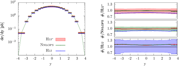
Figure 1: Rapidity of the Higgs boson as predicted by the Hjj-Minlo (Hjj, blue), Nnlops (dark green) and improved Hjj-Minlo ($\textsc{Hjj}^{\star}$, red) generators.

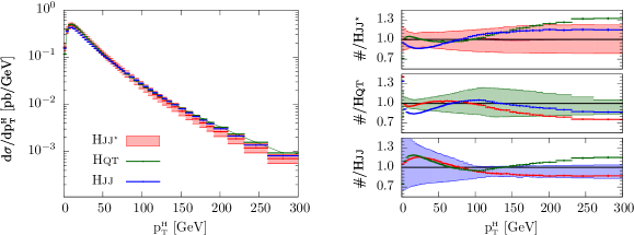
Figure 2: Transverse momentum of the Higgs boson as obtained from the Hjj-Minlo (Hjj, blue) and improved Hjj-Minlo ($\textsc{Hjj}^{\star}$, red) generators, together with the associated NNLL+NNLO computation from the Hqt program (dark green) Bozzi:2003jy ; Bozzi:2005wk ; deFlorian:2011xf .

In figure 2 we plot the Higgs boson transverse momentum spectrum. As with the Higgs boson rapidity distribution no cuts have been applied to the final state. Exceptionally, in this figure we compare $\textsc{Hjj}{}^{\star}$ and Hjj to the NNLL+NNLO predictions of the Hqt program Bozzi:2003jy ; Bozzi:2005wk ; deFlorian:2011xf ; deFlorian:2012mx ; Grazzini:2013mca , instead of Nnlops. Comparing Nnlops (not shown) and $\textsc{Hjj}^{\star}$ we find the two generators agree with one another to within $3\%$ throughout the spectrum, except for the region $p_{{\scriptscriptstyle\mathrm{T}}}\lesssim 5\,\mathrm{GeV}$, where the difference rises up to $15\%$ in the $p_{{\scriptscriptstyle\mathrm{T}}}<2\,\mathrm{GeV}$ region. The latter differences owe to the finite size of the bins in our interpolation grids, coupled with the fact that the distribution is changing very rapidly for $p_{{\scriptscriptstyle\mathrm{T}}}\lesssim 5\,\mathrm{GeV}$. Given this technicality, and the fact that this region is under poor theoretical control anyway, the conclusion, again, is that the method and its implementation work well. Turning then to the comparison with Hqt in figure 2, we see, pleasingly, that the method substantially corrects the shape of the pre-existing Hjj-Minlo simulation, with the resulting $\textsc{Hjj}{}^{\star}$ prediction agreeing very well with Hqt in the region where the latter is undeniably the superior calculation ($p_{{\scriptscriptstyle\mathrm{T}}}\lesssim 100\,\mathrm{GeV}$). In the high transverse momentum tail both $\textsc{Hjj}{}^{\star}$ and Hqt computations have the same NLO accuracy for this distribution. Differences between $\textsc{Hjj}{}^{\star}$ and Hqt occur there due to the different choice of scales in each code, roughly, $p_{{\scriptscriptstyle\mathrm{T}}}^{{\scriptscriptstyle\mathrm{H}}}$ in the case of $\textsc{Hjj}{}^{\star}$, compared to $\frac{1}{2}m_{{\scriptscriptstyle\mathrm{H}}}$ in Hqt. The same comments made above for the Higgs boson rapidity distribution in regards to the uncertainty associated with the $\rho$ parameter apply equally well again here.

Jet cross sections

In figure 3 we compare predictions for inclusive jet cross sections, between the Hjj (blue), Nnlops (dark green) and $\textsc{Hjj}^{\star}$ (red) generators, defined according to the anti-$k_{t}$-jet algorithm Cacciari:2008gp with radius parameter $R=0.4$, for jet transverse momentum thresholds of $25$, $50$ and $100$ GeV. In figure 4 we show the analogous set of plots for the corresponding exclusive jet cross sections. No rapidity cuts have been applied to the jets in making these plots.

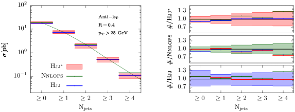
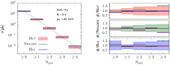
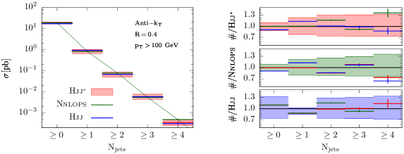
Figure 3: Inclusive jet cross sections, for jets defined according to the anti-$k_{t}$-jet algorithm Cacciari:2008gp with jet radius $R=0.4$. In the upper, middle and lower plots jets are defined for transverse momentum thresholds of $25$, $50$ and $100$ GeV, respectively. In each case we compare output from the Hjj-Minlo (Hjj, blue), Nnlops (dark green) and improved Hjj-Minlo ($\textsc{Hjj}^{\star}$, red) generators.

First we discuss the inclusive jet cross sections in fig. 3. For the 0-jet inclusive cross sections, the improved $\textsc{Hjj}^{\star}$ results are indistinguishable from the Nnlops ones, shifted upwards by 10% with respect to the original Hjj-Minlo predictions (Hjj). The 1-jet inclusive predictions show the $\textsc{Hjj}^{\star}$ results agreeing with the Nnlops ones to within 2%. Unlike the case of the 0-jet bin, in the 1-jet bin, for 25 and 50 GeV jet $p_{{\scriptscriptstyle\mathrm{T}}}$ thresholds, the unimproved Hjj-Minlo result was already in agreement with the Nnlops at the level of 5% or better. So, for the 1-jet inclusive cross sections the room for improvement is very much smaller, with only a small amount visible in the case of the 50 GeV $p_{{\scriptscriptstyle\mathrm{T}}}$ cut. For the case of the 100 GeV jet $p_{{\scriptscriptstyle\mathrm{T}}}$ threshold the unimproved Hjj-Minlo prediction is 10-15% away from the Nnlops one, whereas the improved $\textsc{Hjj}^{\star}$ result sits on top of it. Looking to the higher multiplicity bins, involving at least two jets, we see, as desired, the $\textsc{Hjj}^{\star}$ predictions and those of the parent, unimproved, Hjj-Minlo simulation are in perfect agreement, but for a statistical fluctuation in the 4-jet inclusive cross section with a 100 GeV jet $p_{{\scriptscriptstyle\mathrm{T}}}$ cut. We remind that the vertical error bars indicate statistical errors, which are rarely visible, whereas the shaded bands indicate theoretical uncertainties.

The behaviour seen in all of the inclusive jet cross sections of fig. 3, is as we would naively expect it to be. By construction, our improved Minlo method should reproduce Nnlops results essentially identically for 0- and 1-jet inclusive quantities (eqs. 36-37), while observables that receive their leading contributions from higher jet multiplicities are to be described as in the original Hjj-Minlo generator, which yields the more accurate predictions for those observables.

Given that our Minlo improvement method is intended to return the 0-jet and 1-jet inclusive results of its ‘target’ Nnlops simulation, essentially without ambiguities, one might be tempted to ask why we can see even 2% differences between the Nnlops and $\textsc{Hjj}^{\star}$ predictions for the 1-jet inclusive cross sections. What the improvement procedure precisely does, without ambiguities, assuming a perfect implementation, is to have the improved $\textsc{Hjj}^{\star}$ result reproduce the Nnlops underlying Born kinematics $\Phi_{{\scriptscriptstyle\mathcal{B}\mathrm{J}}}$ (eqs. 36-37) which are defined by clustering events with the exclusive $k_{t}$-jet algorithm, with $R=1.0$. What is plotted in the 1-jet bins of fig. 3 is therefore not in one-to-one correspondence with the kinematics $\Phi_{{\scriptscriptstyle\mathcal{B}\mathrm{J}}}$ (consisting of a Higgs boson and a single pseudoparton in the final-state) but rather it is something which is also sensitive to additional radiation. The $\textsc{Hjj}^{\star}$ and Nnlops generators are further in agreement as to the relative distribution of this additional radiation at the level of $\bar{\alpha}_{{\scriptscriptstyle\mathrm{S}}}^{4}$ terms, i.e. at the level of NLO corrections to Hj, however, at $\mathcal{O}(\bar{\alpha}_{{\scriptscriptstyle\mathrm{S}}}^{5})$ differences do enter. Hence, even if the implementation were a perfect representation of our method, with infinite resolution in the $\Phi_{{\scriptscriptstyle\mathcal{B}\mathrm{J}}}$ grids, we can still expect to see differences between the Nnlops results and $\textsc{Hjj}^{\star}$, for the 1-jet inclusive cross section, which are formally NNLO-sized in the context of the inclusive 1-jet calculation. This being the case, one can be quite satisfied with only 2% differences between the Nnlops and $\textsc{Hjj}^{\star}$ predictions for the 1-jet inclusive cross sections. In fact, we examined the 0- and 1-jet inclusive cross sections, with a 25 GeV jet $p_{{\scriptscriptstyle\mathrm{T}}}$ threshold, prior to interfacing with the parton shower, whereupon we found the 0-jet and 1-jet $\textsc{Hjj}^{\star}$ cross sections to be indistinguishable from their Nnlops counterparts, while the 2- and 3-jet bins remained identical to those of Hjj-Minlo.

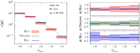
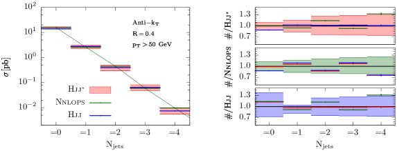
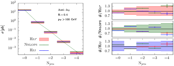
Figure 4: Exclusive jet cross sections, for jets defined according to the anti-$k_{t}$-jet algorithm Cacciari:2008gp with jet radius $R=0.4$. In the upper, middle and lower plots jets are defined for transverse momentum thresholds of $25$, $50$ and $100$ GeV, respectively. In each case we compare output from the Hjj-Minlo (Hjj, blue), Nnlops (dark green) and improved Hjj-Minlo ($\textsc{Hjj}^{\star}$, red) generators.

Let us now turn our attention to the exclusive jet cross sections of fig. 4. First, for the high multiplicity bins, involving two or more jets, the $\textsc{Hjj}^{\star}$ results are in complete agreement with those of its parent unimproved Hjj-Minlo generator (up to a single statistical fluctuation). The Nnlops predictions are nominally only LO accurate for the $2$-jet bins, whereas for higher jet multiplicity bins the simulation relies entirely on the parton shower approximation. The Hjj and $\textsc{Hjj}^{\star}$ predictions, on the other hand, are expected to be NLO accurate for the 2-jet bins, LO for the 3-jet bins, only resorting to the parton shower approximation in the 4-jet bins. $\textsc{Hjj}^{\star}$ being in perfect agreement with Hjj-Minlo for the latter cross sections is, of course, the desired behaviour from our improved Minlo prediction.

For the 0-jet exclusive cross sections in fig. 4 we see nice agreement between the $\textsc{Hjj}^{\star}$ and Nnlops predictions at the 1-2% level or better, as is to be expected by construction of our method. To explain the 1-2% differences that can be seen we tender again the same theoretical explanation as above (the Nnlops and $\textsc{Hjj}^{\star}$ results differ, by construction, at the level of $\mathcal{O}(\bar{\alpha}_{{\scriptscriptstyle\mathrm{S}}}^{5})$ terms), however, with such small differences we also cannot rule out imperfections in the implementation, e.g. artefacts due to the finite granularity of the grids and grid interpolation. We suffice to say that the differences between the $\textsc{Hjj}^{\star}$ and Nnlops computations of the 0-jet exclusive cross sections are negligibly small, while the unimproved Hjj-Minlo result sits 10-15% below them.

Lastly, we look to the the 1-jet exclusive cross sections. The plots in this case read that the $\textsc{Hjj}^{\star}$ prediction is different from the Nnlops one by 7% for the 25 GeV jet $p_{{\scriptscriptstyle\mathrm{T}}}$ threshold, 5% for the 50 GeV threshold, and $\sim 0\%$ for the 100 GeV threshold. Meanwhile, the unimproved Hjj-Minlo prediction is in agreement with the Nnlops prediction at the level of $\sim 0$%, 10%, and 15%, for the same $p_{{\scriptscriptstyle\mathrm{T}}}$ thresholds, respectively.

Since the Minlo improvement method we propose works to correct the inclusive 0- and 1-jet Hjj-Minlo cross sections to be equal to those of the target Nnlops generator, while leaving inclusive 2-jet observables basically untouched, we consider it can be useful to think of the exclusive 1-jet cross section as the difference of the inclusive 1- and 2-jet cross sections: $\sigma\left(=1-\mathrm{jet}\right)=\sigma\left(\geq 1-\mathrm{jet}\right)-\sigma\left(\geq 2-\mathrm{jets}\right)$. Clearly if $\sigma\left(\geq 1-\mathrm{jet}\right)\gg\sigma\left(\geq 2-\mathrm{jets}\right)$ differences in the latter will have limited impact on the exclusive 1-jet cross section. The latter scenario is enhanced by increasing the jet $p_{{\scriptscriptstyle\mathrm{T}}}$ threshold and, sure enough, the pattern of the exclusive jet-cross sections seen in the case of the 100 GeV $p_{{\scriptscriptstyle\mathrm{T}}}$ threshold, mirrors well what we see in the analogous inclusive jet cross section case, discussed overhead. To explain then the differences seen between the Nnlops and $\textsc{Hjj}^{\star}$ generators at the 25 GeV and 50 GeV jet $p_{{\scriptscriptstyle\mathrm{T}}}$ thresholds, we note that the Nnlops exclusive 1-jet cross section is given by its inclusive 1-jet cross section minus its inclusive 2-jet cross section, on the other hand, by design, as can be verified in fig. 3, the $\textsc{Hjj}^{\star}$ exclusive 1-jet cross section is basically given by the Nnlops inclusive 1-jet cross section minus the Hjj-Minlo inclusive 2-jet cross section. Since the Hjj-Minlo inclusive 2-jet cross section at the 25 GeV jet $p_{{\scriptscriptstyle\mathrm{T}}}$ thresholds is 10% lower than the Nnlops one, while the ratio of the inclusive 1-jet to 2-jet cross sections is roughly two, it follows that one can expect the $\textsc{Hjj}^{\star}$ 1-jet exclusive cross section to be 5% higher than the corresponding Nnlops one. Adding in the fact that the $\textsc{Hjj}^{\star}$ 1-jet inclusive cross section was already 1-2% above the corresponding Nnlops one, the 7% excess is actually very much in line with expectations based on how the method is intended to work, in particular, its preserving of the inclusive cross sections. A similar explanation holds for the 50 GeV jet $p_{{\scriptscriptstyle\mathrm{T}}}$ threshold result, however, there the fact that the 2-jet inclusive cross section of Hjj-Minlo is low does not imply as big an increase is needed in the 1-jet exclusive bin to recover the 1-jet inclusive Nnlops result, since for that higher $p_{{\scriptscriptstyle\mathrm{T}}}$ threshold $\sigma\left(\geq 1-\mathrm{jet}\right)\gg\sigma\left(\geq 2-\mathrm{jets}\right)$. We also remark that the $\textsc{Hjj}^{\star}$ exclusive 1-jet cross section results all agree with those of the Nnlops generator to within the thickness of the scale uncertainty bands.

We finally note that the dark-red scale uncertainty band associated to variation of the $\rho$ parameter, as described in sects. 4.1-4.2, is invisible here: the effect of varying this parameter on these distributions is totally negligible.

To conclude the discussion on jet cross sections, we can say that all of the results we find are very much in line with expectations regarding how our method should function, all vindicating the method and its implementation.

Leading jet

In figures 5-9 we plot various quantities relating to the kinematics of the leading jet. In all of these figures jets have been defined according to the anti-$k_{t}$ clustering algorithm, with jet radius $R=0.4$; no rapidity cuts have been applied to the jets. For figs. 7, 8, 9 jets were further defined as having a transverse momentum of at least 25 GeV.

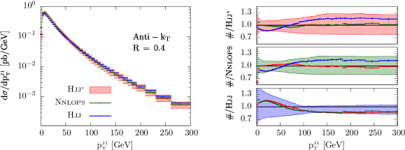
Figure 5: Leading jet transverse momentum spectrum, for anti-$k_{t}$-jets with radius parameter $R=0.4$.

The results for the leading jet transverse momentum spectrum in fig. 5 read similarly to those reported for the Higgs boson transverse momentum spectrum (fig. 2). The Nnlops and $\textsc{Hjj}^{\star}$ predictions agree very well throughout the spectrum, with the procedure correcting well for substantial ($\pm 15\%$) shape differences between the unimproved Hjj-Minlo result and the more accurate Nnlops prediction. Regarding differences between the Nnlops and $\textsc{Hjj}^{\star}$ results in the $p_{{\scriptscriptstyle\mathrm{T}}}\lesssim 5\,\mathrm{GeV}$ region, the explanation here is the same as for the case of the Higgs boson $p_{{\scriptscriptstyle\mathrm{T}}}$ spectrum, namely, that the granularity in our discretized implementation of the $\Phi_{{\scriptscriptstyle\mathcal{B}\mathrm{J}}}$ phase space is not sufficiently fine to cope with the rapidly changing distribution for $p_{{\scriptscriptstyle\mathrm{T}}}\lesssim 5\,\mathrm{GeV}$. We reiterate that this region is under limited theoretical control anyway. Indeed, rather than seek improved agreement of Nnlops and $\textsc{Hjj}^{\star}$ in the latter murky region, we might prefer to lessen the 3-5% deviation in the neighbourhood $60\leq p_{{\scriptscriptstyle\mathrm{T}}}\leq 80$ GeV. This region, where the Hjj-Minlo and Nnlops lines intersect, appears to be where the $p_{{\scriptscriptstyle\mathrm{T}}}$ derivative of the difference between the two predictions is changing most rapidly, i.e. the numerator of $\delta\left(\Phi_{{\scriptscriptstyle\mathcal{B}\mathrm{J}}}\right)$ in eq. 31/47. It should therefore be possible to improve agreement between the Nnlops and $\textsc{Hjj}^{\star}$ results in this region by, for example, making use of (irregular) optimized grids and interpolation methods which can work on them. Overall, notwithstanding our unsophisticated implementation, agreement between the Nnlops and $\textsc{Hjj}^{\star}$ predictions is very satisfactory, providing significant improvement across the whole $p_{{\scriptscriptstyle\mathrm{T}}}$ spectrum relative to the original Hjj-Minlo generator.

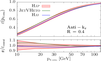
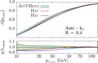
Figure 6: The jet veto efficiency, $\varepsilon(p_{{\scriptscriptstyle\mathrm{T,veto}}})$, is defined as the cross section for Higgs boson production events containing no jets with transverse momentum greater than $p_{{\scriptscriptstyle\mathrm{T,veto}}}$, divided by the respective total inclusive cross section. Jets are defined here according to the anti-$k_{t}$-jet algorithm with $R=0.4$. On the left, in the red shaded area, one can see the scale uncertainty band obtained from the improved Hjj-Minlo ($\textsc{Hjj}^{\star}$) simulation, with the NNLL+NNLO prediction from the JetVHeto program Banfi:2012yh ; Banfi:2012jm overlaid in green, and that of the original Hjj-Minlo program in blue. The lower pane displays the same quantities as a ratio with respect to the central $\textsc{Hjj}^{\star}$ prediction. On the right we display instead the corresponding uncertainty band obtained from JetVHeto (i.e. renormalization and factorization scale variations only), with the central value of the JetVHeto prediction defining the reference line in the associated ratio plot.

In fig. 6 we plot Hjj, $\textsc{Hjj}^{\star}$ and NNLL+NNLO JetVHeto Banfi:2012yh ; Banfi:2012jm predictions for the jet veto efficiency, $\varepsilon(p_{{\scriptscriptstyle\mathrm{T,veto}}})$, defined as the cross section for Higgs boson production events containing no jets with transverse momentum greater than $p_{{\scriptscriptstyle\mathrm{T,veto}}}$, divided by the respective total inclusive cross section. In the left-hand column, in the red shaded area, we show the scale uncertainty band predicted by the $\textsc{Hjj}^{\star}$ simulation, with the central NNLL+NNLO resummed prediction of JetVHeto superimposed in green (matching scheme-(a), $\mu_{{\scriptscriptstyle\mathrm{R}}}=\mu_{{\scriptscriptstyle\mathrm{F}}}=\mu_{{\scriptscriptstyle\mathrm{Q}}}=m_{{\scriptscriptstyle\mathrm{H}}}$, $\mu_{{\scriptscriptstyle\mathrm{Q}}}$ being the resummation scale). The lower panel shows the ratio with respect to the $\textsc{Hjj}^{\star}$ prediction obtained with its central scale choice. On the right we have made the same plots as on the left but with the JetVHeto predictions replacing those of the $\textsc{Hjj}^{\star}$ and vice-versa. The uncertainty band in the JetVHeto results is the envelope of a seven point variation of $\mu_{{\scriptscriptstyle\mathrm{R}}}$ and $\mu_{{\scriptscriptstyle\mathrm{F}}}$ by a factor of two. This is in contrast to the band associated with it in ref. Banfi:2012jm , where additionally resummation scale and matching scheme variations were included in the envelope. Thus the JetVHeto error band here is considerably smaller than that shown in ref. Banfi:2012jm . We restricted the JetVHeto uncertainty estimate to the same class of variations so as to have a more like-for-like comparison to the $\textsc{Hjj}^{\star}$ band.

The $\textsc{Hjj}^{\star}$ and JetVHeto predictions agree within the $\textsc{Hjj}^{\star}$ uncertainties, but not quite to within the thickness of the restricted JetVHeto band, in which case the central $\textsc{Hjj}^{\star}$ prediction is 1-2% below the lower edge of the uncertainty band. Nevertheless, considering the JetVHeto calculation has superior accuracy to both the $\textsc{Hjj}^{\star}$ and Nnlops predictions, through its high accuracy resummation, the level of agreement we find should be understood as being, again, quite satisfactory: the $\textsc{Hjj}^{\star}$ prediction is always within 5% of the JetVHeto result, moreover, for the region $p_{{\scriptscriptstyle\mathrm{T},\mathrm{veto}}}>25$ GeV, it is within 3% of the JetVHeto prediction. We also observed that if we compare to the JetVHeto results with the same uncertainty prescription as ref. Banfi:2012jm (not shown), the central $\textsc{Hjj}^{\star}$ prediction lies within half the thickness of the more conservative error band that results in that case.

In ref. Hamilton:2013fea we presented results showing the Nnlops prediction lying within 1-2% of the JetVHeto prediction, over the full $p_{{\scriptscriptstyle\mathrm{T},\mathrm{veto}}}$ range. Some degree of that good agreement stemmed from exploiting freedom in the distribution of the NNLO-to-NLO inclusive K-factor across the leading jet $p_{{\scriptscriptstyle\mathrm{T}}}$ spectrum, to ‘tune’ the Nnlops result. We expect that the slightly less good agreement in the $\textsc{Hjj}^{\star}$ result here is correlated with the percent level differences seen above in our jet $p_{{\scriptscriptstyle\mathrm{T}}}$ spectrum, between $\textsc{Hjj}^{\star}$ and Nnlops. We remind that these differences are technical in origin, and should be entirely removable with a more refined implementation of our method.

Lastly, we remark that the unimproved Hjj-Minlo results for the jet veto efficiency are, somewhat surprisingly, also quite good. This good agreement of unimproved Hjj-Minlo and JetVHeto is, however, rather fortuitous. The 0-jet cross section in the numerator of the definition of the jet veto efficiency, is equal to the $p_{{\scriptscriptstyle\mathrm{T}}}$ integral of the leading jet transverse momentum spectrum from $p_{{\scriptscriptstyle\mathrm{T}}}=0$ GeV up to $p_{{\scriptscriptstyle\mathrm{T}}}=p_{{\scriptscriptstyle\mathrm{T,veto}}}$. One can clearly see from figure 5 that the leading jet transverse momentum spectrum from the unimproved Hjj-Minlo generator is, in general, quite different with respect to the Nnlops and improved $\textsc{Hjj}^{\star}$ results. For the region $p_{{\scriptscriptstyle\mathrm{T},\mathrm{veto}}}\lesssim 30$ GeV the $\textsc{Hjj}^{\star}$ and unimproved Hjj-Minlo jet $p_{{\scriptscriptstyle\mathrm{T}}}$ spectra, while clearly different in normalization, are actually not so different in shape. By definition, the jet veto efficiency, $\varepsilon(p_{{\scriptscriptstyle\mathrm{T,veto}}})$, divides out the respective total cross sections, and hence it is therefore reasonable to expect $\varepsilon(p_{{\scriptscriptstyle\mathrm{T,veto}}})$ is not so different in the $\textsc{Hjj}^{\star}$ and unimproved Hjj-Minlo predictions for the latter $p_{{\scriptscriptstyle\mathrm{T},\mathrm{veto}}}$ region. Moreover, since the numerator of $\varepsilon(p_{{\scriptscriptstyle\mathrm{T,veto}}})$ is the cumulant of the leading jet transverse momentum spectrum, which receives, by far, its main contribution from the low $p_{{\scriptscriptstyle\mathrm{T}}}$ region, it follows that the behaviour of $\varepsilon(p_{{\scriptscriptstyle\mathrm{T,veto}}})$, for $p_{{\scriptscriptstyle\mathrm{T},\mathrm{veto}}}\gtrsim 30$ GeV, is less sensitive to differences in the latter spectrum in this region, with all predictions converging steadily towards $\varepsilon(m_{{\scriptscriptstyle\mathrm{H}}})\approx 1$.

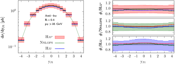
Figure 7: Leading jet rapidity for anti-$k_{t}$-jets with radius parameter $R=0.4$ and a transverse momentum threshold of $25$ GeV.

Figure 7 shows the rapidity of the leading $R=0.4$ anti-$k_{t}$ jet, with a 25 GeV cut on the jet transverse momentum. Broadly speaking the structure of the results in this distribution, in particular their normalization, can be explained in terms of the inclusive 1-jet cross section with the same jet $p_{{\scriptscriptstyle\mathrm{T}}}$ threshold; the uppermost plot at the top of fig. 3. We remind that the Hjj-Minlo prediction for this observable is nominally LO, whereas the Nnlops and $\textsc{Hjj}^{\star}$ results are NLO accurate. This being the case, it is a remarkable coincidence that the unimproved Hjj-Minlo result only exhibits very small differences with respect to the other two predictions, at the level of about 5%.

The Nnlops and $\textsc{Hjj}^{\star}$ results are almost indistinguishable in the central rapidity region, with the $\textsc{Hjj}^{\star}$ prediction improved in this aspect, relative to its parent Hjj-Minlo simulation. Towards the higher rapidity regions, differences in the Nnlops and $\textsc{Hjj}^{\star}$ results, on the level of $\sim 5\%$, become visible. Generally speaking the $\mathrm{y}_{{\scriptscriptstyle\mathrm{J}1}}$ distributions of $\textsc{Hjj}^{\star}$ and its parent Hjj-Minlo generator, exhibit very slight, and very similar, ‘smiles’ with respect to the Nnlops distribution. In the Hjj-Minlo case the ‘smile’ feature coupled with its smaller inclusive 1-jet cross section conspires to make it agree very well with the Nnlops prediction in the high rapidity regions, where the improved $\textsc{Hjj}^{\star}$ program is off by 5%.

We refer back to the discussion of the inclusive 1-jet cross section, surrounding fig. 3, for comments on why one can expect to see small deviations between the $\textsc{Hjj}^{\star}$ result and the target Nnlops distribution for general inclusive 1-jet quantities, starting at the level of $\bar{\alpha}_{{\scriptscriptstyle\mathrm{S}}}^{5}$ terms. Our initial reaction, to seeing the difference in shape between the $\mathrm{y}_{{\scriptscriptstyle\mathrm{J}1}}$ distributions of the $\textsc{Hjj}^{\star}$ and Nnlops results, was to interpret it as being due to a weakness in our implementation of our method. Re-making this distribution at the level of the $\textsc{Hjj}^{\star}$ and Nnlops LHE events reveals, however, that the two are actually indistinguishable from one another (the distributions agree at the sub-percent level). Moreover, at the LHE level, the unimproved Hjj-Minlo code is more clearly out of agreement with both of the latter and, in particular, it does no longer agree so well with and the Nnlops in the high rapidity region; the difference being at the level of 5%.

It follows that our implementation of the method actually works perfectly as intended, and that the small features above which were counter to naive expectations, are actually fully attributable to the attachment of the parton shower. The parton shower generates the 3rd hardest radiation and beyond in the Nnlops generator, while it starts by generating the 4th hardest radiation in the case of Hjj-Minlo and $\textsc{Hjj}^{\star}$. Naturally then the effect of the parton shower on the $\mathrm{y}_{{\scriptscriptstyle\mathrm{J}1}}$ distribution in the Nnlops case is greater, acting to deplete the cross section in the high rapidity side bands relative to the Hjj-Minlo and $\textsc{Hjj}^{\star}$ results. Given that the difference between the theoretically superior $\textsc{Hjj}^{\star}$ and Nnlops results in these high rapidity regions has been traced to the effects of the 3rd hardest emitted parton (i.e. an $\bar{\alpha}_{{\scriptscriptstyle\mathrm{S}}}^{5}$ effect), we cannot say one result is better than the other. We suffice to say that the difference is in any case small, in a region where theoretical control is not as high as in other places, and it is very much contained within the scale uncertainty bands.

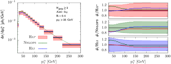
Figure 8: Leading jet transverse momentum in events with two or more jets; jets are here defined according to the anti-$k_{t}$ algorithm with radius $R=0.4$ and a transverse momentum threshold of $25$ GeV.

Figure 8 shows the transverse momentum spectrum of the leading jet, in events containing at least two $R=0.4$ anti-$k_{t}$ jets, with transverse momenta above 25 GeV. Ostensibly, this is a rather everyday observable, but it nevertheless probes Sudakov effects on the $y_{12}$ distribution. So, it is really the first distribution we have shown so far which is sensitive to non-trivial workings of our method. Towards the low end of the spectrum, $p_{{\scriptscriptstyle\mathrm{T}}}^{{\scriptscriptstyle\mathrm{J}1}}\lesssim 75$ GeV, there is essentially not enough phase space available to generate large $L_{12}$ logarithms. By contrast, at the high $p_{{\scriptscriptstyle\mathrm{T}}}^{{\scriptscriptstyle\mathrm{J}1}}$ end, one can expect large $L_{12}$ logarithms, with a significant contribution from events for which $\sqrt{y_{12}}\gtrsim 25$ GeV and $\sqrt{y_{01}}$ is of the order of $p_{{\scriptscriptstyle\mathrm{T}}}^{{\scriptscriptstyle\mathrm{J1}}}$. So, even though the distribution is defined on 2-jet events, in the high $p_{{\scriptscriptstyle\mathrm{T}}}^{{\scriptscriptstyle\mathrm{J1}}}$ limit, the second jet should generally be considered as secondary, soft, radiation emitted from a hard, high-$p_{{\scriptscriptstyle\mathrm{T}}}$, Higgs-plus-jet system.

By construction our method will only act to correct the Hjj-Minlo distribution for $y_{01}\gg y_{12}$, leaving regions where there is no such strong scale hierarchy untouched. Thus, in fig. 8, at low transverse momentum, we see the $\textsc{Hjj}^{\star}$ distribution agrees identically with Hjj-Minlo. This is, of course, the desired behaviour, since in this region, for this (2-jet) observable, Hjj-Minlo is nominally NLO accurate, whereas Nnlops is only LO. We remind that, the analogous inclusive leading jet transverse momentum spectrum, fig. 3, displays significant deviations in shape between Nnlops/$\textsc{Hjj}^{\star}$ and Hjj-Minlo in this same $p_{{\scriptscriptstyle\mathrm{T}}}$ region, while Nnlops and $\textsc{Hjj}^{\star}$ are in near perfect agreement.

Turning instead to the high $p_{{\scriptscriptstyle\mathrm{T}}}^{{\scriptscriptstyle\mathrm{J}1}}$ region, the three predictions are in good agreement with one another. In the high $p_{{\scriptscriptstyle\mathrm{T}}}^{{\scriptscriptstyle\mathrm{J}1}}$ region there is perhaps a faint hint of the $\textsc{Hjj}^{\star}$ result tending to that of the Nnlops. We assert that the latter tendency would be the correct and desirable result there. Should the transverse momentum of the leading jet enter a high enough $p_{{\scriptscriptstyle\mathrm{T}}}$ regime, a 25 GeV jet-defining $p_{{\scriptscriptstyle\mathrm{T}}}$ cut for the second jet will correspond to a cut deep in the Sudakov region of the corresponding $\sqrt{y_{12}}$ distribution, in which case, the leading jet $p_{{\scriptscriptstyle\mathrm{T}}}$ spectrum in two-jet events increasingly corresponds to the inclusive leading jet $p_{{\scriptscriptstyle\mathrm{T}}}$ spectrum.

Finally for fig. 8, we notice that the dark red band, depicting uncertainty due to variations of the technical $\rho$ parameter, has become visible for the first time in this section (in the upper-right ratio plot, at high transverse momentum). This technical systematic is, however, seemingly limited to a $\pm 2\%$ uncertainty, which is dwarfed by the conventional theoretical uncertainty coming from the renormalization and factorization scale variations (the significantly larger light-red band).

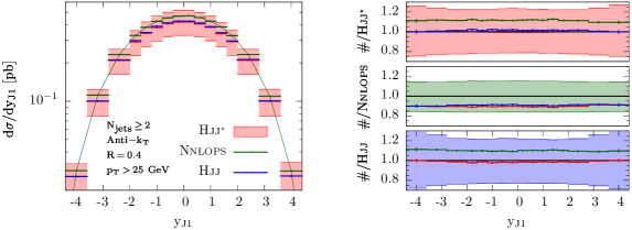
Figure 9: Leading jet rapidity in events with two or more anti-$k_{t}$, $R=0.4$, $p_{{\scriptscriptstyle\mathrm{T}}}\geq 25\,\mathrm{GeV}$ jets.

The last distribution we present showing the behaviour of the leading jet is that of its rapidity in events with at least two-jets, fig. 9. This distribution is rather unremarkable given what we have shown immediately before, for the leading jet transverse momentum spectrum in the same class of events (fig. 8). Here, as in fig. 8, the distribution shows that the $\textsc{Hjj}^{\star}$ distribution overlaps the Hjj-Minlo prediction, which is NLO accurate in the descriptions of this observable, while the Nnlops result is only LO. This is the expected and, of course, the desired behaviour of our improved $\textsc{Hjj}^{\star}$ simulation.

Second jet and third hardest jets

In this subsection we move to present plots of distributions probing directly the behaviour of the second and third hardest jets produced in association with the Higgs boson. As before, jets have been defined according to the anti-$k_{t}$ clustering algorithm, with the jet radius parameter $R=0.4$. Additionally, for the case of jet rapidity distributions, in figures 12 and 13, the jets are required to pass a transverse momentum threshold of 25 GeV.

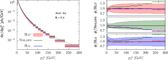
Figure 10: Transverse momentum spectrum of the second jet.

The transverse momentum spectrum of the second hardest jet is plotted in fig. 10. In all simulations, before (not shown) and after showering, the distribution peaks in the bin at $3\,\mathrm{GeV}\leq p_{{\scriptscriptstyle\mathrm{T}}}^{{\scriptscriptstyle\mathrm{J}2}}\leq\,6\,\mathrm{GeV}$. Moving upwards from the first bin at $p_{{\scriptscriptstyle\mathrm{T}}}^{{\scriptscriptstyle\mathrm{J}2}}=0$ GeV the $\textsc{Hjj}^{\star}$ (red) and Hjj-Minlo (blue) predictions start off with a 20% difference, which smoothly and monotonically diminishes, with the two distributions coalescing at $p_{{\scriptscriptstyle\mathrm{T}}}^{{\scriptscriptstyle\mathrm{J}2}}\approx 20$ GeV. For higher transverse momenta, the $\textsc{Hjj}^{\star}$ and Hjj-Minlo histograms become indistinguishable from one another. Meanwhile, in the same region, the Nnlops result starts off with a 15% discrepancy between it and the latter simulations, which rises with the transverse momentum. Nevertheless, the Nnlops prediction is within the margins set by all renormalization and factorization scale uncertainty bands.

The behaviour of the $\textsc{Hjj}^{\star}$ and Hjj-Minlo predictions relative to one another is as intended. In general, the Hjj-Minlo prediction is NLO accurate in the description of $p_{{\scriptscriptstyle\mathrm{T}}}^{{\scriptscriptstyle\mathrm{J2}}}$, and so it is of course desirable that the $\textsc{Hjj}^{\star}$ tends to that result in regions where Sudakov logarithms at higher orders are not large, i.e. away from the Sudakov peak. In the vicinity of the peak, large logarithms enter at every order in perturbation theory. In this feasibility study we claim to control these large logarithms nominally at just LL/$\mathrm{NLL}_{\sigma}$ accuracy. The improved $\textsc{Hjj}^{\star}$ prediction works so as to implement unitarity for the 0- and 1-jet inclusive cross sections by ascribing the mismatch there to missing $\mathrm{NNLL}_{\sigma}$ Sudakov logarithms beyond NLO. The increasing difference of $\textsc{Hjj}^{\star}$ with respect to Hjj-Minlo in the region $p_{{\scriptscriptstyle\mathrm{T}}}^{{\scriptscriptstyle\mathrm{J}2}}\leq 20$ GeV, up onto the Sudakov peak, roughly reflects this $\mathrm{NNLL}_{\sigma}$ ‘profiling’ of the $\sim$10-12% excess in the Nnlops total inclusive cross section over that of Hjj-Minlo (see e.g. figs. 1-3).

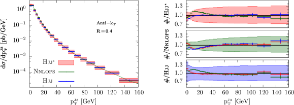
Figure 11: Third jet transverse momentum spectrum.

In figure 11 we plot the transverse momentum of the third jet. In this case there is, coincidentally, good agreement of all predictions in the moderate to high $p_{{\scriptscriptstyle\mathrm{T}}}$ domain. This is somewhat fortuitous in the context of the Nnlops simulation, since the third jet in that simulation is generated exclusively in the parton shower approximation, whereas in $\textsc{Hjj}^{\star}$ and Hjj-Minlo it has a matched matrix element-parton shower description. With a view to validating our ideas, what is more relevant is the observation of the relative behaviour of $\textsc{Hjj}^{\star}$ and Hjj-Minlo. Here we see, essentially, exactly the same trend as found in the case of $p_{{\scriptscriptstyle\mathrm{T}}}^{{\scriptscriptstyle\mathrm{J}2}}$, specifically, identical agreement for $p_{{\scriptscriptstyle\mathrm{T}}}^{{\scriptscriptstyle\mathrm{J}2}}\gtrsim 10-15$ GeV, with a steadily increasing excess of $\textsc{Hjj}^{\star}$ over Hjj-Minlo as one looks towards zero transverse momentum. These aspects are also fully explained and intended, with the same reasoning as for $p_{{\scriptscriptstyle\mathrm{T}}}^{{\scriptscriptstyle\mathrm{J}2}}$. The only slight difference here is that the third jet being, by definition, softer than the second jet, implies that the excess of $\textsc{Hjj}^{\star}$ over Hjj-Minlo is confined to a slightly lower region of the $p_{{\scriptscriptstyle\mathrm{T}}}^{{\scriptscriptstyle\mathrm{J}3}}$ distribution, than one finds in the $p_{{\scriptscriptstyle\mathrm{T}}}^{{\scriptscriptstyle\mathrm{J}2}}$ case.

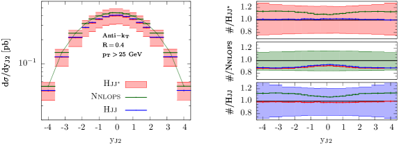
Figure 12: Rapidity of the second hardest jet.

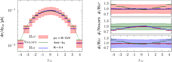
Figure 13: Rapidity of the third hardest jet.

Figures 12 and 13 show, respectively, the rapidity spectra of the second and third hardest $R=0.4$ anti-$k_{t}$ jets, with $p_{{\scriptscriptstyle\mathrm{T}}}\geq 25$ GeV. Both figures reveal the $\textsc{Hjj}^{\star}$ results agreeing perfectly with those of the ‘parent’ Hjj-Minlo simulation. The Nnlops predictions clearly differ in shape and normalization with respect to the latter but, nevertheless, they remain within the renormalization and factorization scale uncertainty bands. For what concerns the normalization of the distributions, the perfect agreement between $\textsc{Hjj}^{\star}$ and Hjj-Minlo was to be expected, based on that seen already in the related 2-jet inclusive cross sections (fig. 3). As with the $p_{{\scriptscriptstyle\mathrm{T}}}^{{\scriptscriptstyle\mathrm{J}2}}$ and $p_{{\scriptscriptstyle\mathrm{T}}}^{{\scriptscriptstyle\mathrm{J}3}}$ spectra, for modest values of the transverse momentum, the tendency of $\textsc{Hjj}^{\star}$ to reproduce Hjj-Minlo here is as intended and desired; the latter being NLO accurate for $\mathrm{y}_{{\scriptscriptstyle\mathrm{J}2}}$ and LO accurate for $\mathrm{y}_{{\scriptscriptstyle\mathrm{J}3}}$, in contrast to the LO and parton shower accuracy, respectively, afforded by the Nnlops.

Jet rates

In figures 14 and 15 we present differential jets rates obtained from the exclusive $k_{t}$-jet clustering algorithm with radius parameter $R=1$. Figure 14 shows the $\log_{10}\sqrt{y_{01}}$ and $\log_{10}\sqrt{y_{12}}$ jet rate distributions, while figure 15 shows $\log_{10}\sqrt{y_{23}}$ and $\log_{10}\sqrt{y_{34}}$.

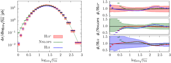
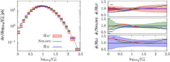
Figure 14: In the upper plots we display the $\log_{10}\sqrt{y_{01}}$ differential jet rate on the left, while on the right we show the various predictions relative to the central improved Hjj-Minlo ($\textsc{Hjj}^{\star}$), Nnlops and original Hjj-Minlo (Hjj) ones, respectively, in the top, middle and bottom panels. In the lower plots we display the corresponding set of distributions for the $\log_{10}\sqrt{y_{12}}$ differential jet rate. In the making of these plots jets have been clustered according to the $k_{t}$-jet algorithm, with radius parameter $R=1$.

The $\log_{10}\sqrt{y_{01}}$ distribution in figure 14 is equivalent to a plot of the transverse momentum of the leading jet in the event, defined according to the $k_{t}$-jet clustering algorithm with $R=1$. It is therefore not surprising to find that the results for this distribution have a markedly similar structure to those for the leading jet transverse momentum spectrum in fig. 5; notwithstanding the fact that in the latter case the jets were defined according to the anti-$k_{t}$ jet algorithm, with radius parameter $R=0.4$. We therefore refer the reader back to the discussion surrounding fig. 5, for further explanation regarding the features of the $\log_{10}\sqrt{y_{01}}$ distribution.

The $\log_{10}\sqrt{y_{12}}$ in fig. 14 is more interesting, since this distribution is directly affected by our proposed Minlo improvement procedure. One can relatively quickly gain an appreciation for the pattern of the results here by noting that there is some reasonable degree of correspondence to be expected between $\sqrt{y_{12}}$ and $p_{{\scriptscriptstyle\mathrm{T}}}^{{\scriptscriptstyle\mathrm{J}2}}$, based on how $\sqrt{y_{12}}$ is defined; if all the jet clustering algorithm did was initial-state clusterings, they would indeed be exactly the same thing. Despite seeming like an over-simplification, it is nevertheless the case that the relative behaviours of the three predictions here are in very good agreement, quantitatively, with that discussed earlier for the $p_{{\scriptscriptstyle\mathrm{T}}}^{{\scriptscriptstyle\mathrm{J}2}}$ spectrum (fig. 10).

As in $p_{{\scriptscriptstyle\mathrm{T}}}^{{\scriptscriptstyle\mathrm{J}2}}$ we see an excess of Nnlops with respect to $\textsc{Hjj}^{\star}$ and Hjj-Minlo of $\sim 12\%$ in the region $20\,\mathrm{GeV}\lesssim\sqrt{y_{12}}\lesssim 100\,\mathrm{GeV}$, with the latter pair of simulations in perfect agreement. For $\sqrt{y_{12}}\lesssim 20\,\mathrm{GeV}$, as in the corresponding region of the $p_{{\scriptscriptstyle\mathrm{T}}}^{{\scriptscriptstyle\mathrm{J}2}}$ distribution, the $\textsc{Hjj}^{\star}$ and Hjj-Minlo predictions become increasingly separate, with the former increasing over the latter, manifesting the restorative effect of the correction procedure to recover the inclusive 0- and 1-jet Nnlops cross sections. Even the crossing over of the Nnlops and $\textsc{Hjj}^{\star}$ distributions appears to occur at exactly the same place in the $p_{{\scriptscriptstyle\mathrm{T}}}^{{\scriptscriptstyle\mathrm{J}2}}$ and $\log_{10}\sqrt{y_{12}}$ distributions ($\sqrt{y_{12}}\sim 9\,\mathrm{GeV}$). In contrast to the $p_{{\scriptscriptstyle\mathrm{T}}}^{{\scriptscriptstyle\mathrm{J}2}}$ distribution, the $\log_{10}\sqrt{y_{12}}$ plot makes it clearer when, and to what extent, the correction kicks-in. One can see that the correction turns on smoothly just before the Sudakov peak, starting at $\log_{10}\sqrt{y_{12}}\approx 1.25$, ($\sqrt{y_{12}}\approx 18\,\mathrm{GeV}$), leading to a 7% increase in $\textsc{Hjj}^{\star}$ over Hjj-Minlo on the Sudakov peak, and ranging up to 25% at $\sqrt{y_{12}}=1\,\mathrm{GeV}$.

Lastly, this $\log_{10}\sqrt{y_{12}}$ distribution shows the first real evidence, so far, of some sensitivity in the $\textsc{Hjj}^{\star}$ results to the technical $\rho$ parameter. The conservatively estimated systematic uncertainty owing to $\rho$ is depicted by the dark-red band, seen superimposed on the light-red band, in the uppermost ratio plot. This sensitivity to $\rho$ is, however, rather contained at the level of $\pm 10-15\%$, moreover, it is basically negligible above $\sqrt{y_{12}}=3\,\mathrm{GeV}$.

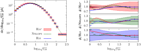
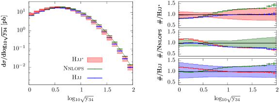
Figure 15: In the upper-left plot we show the $\log_{10}\sqrt{y_{23}}$ jet rate, while on the right we show the various predictions again as ratios with respect to one another. In the lower plots we display the corresponding set of distributions for the $\log_{10}\sqrt{y_{34}}$ jet rate. Jets have been constructed using the $k_{t}$-jet algorithm, with $R=1$.

Moving on, in the upper half of fig. 15 we have the $\log_{10}\sqrt{y_{23}}$ distribution. The correspondence of $\sqrt{y_{12}}$ with $p_{{\scriptscriptstyle\mathrm{T}}}^{{\scriptscriptstyle\mathrm{J}2}}$, which helped to quickly understand the $\log_{10}\sqrt{y_{12}}$ results above, has an analogon here, namely, that neglecting final-state clusterings by the jet algorithm, $\sqrt{y_{23}}$ becomes equal to $p_{{\scriptscriptstyle\mathrm{T}}}^{{\scriptscriptstyle\mathrm{J}3}}$. This analogy continues to appear to hold remarkably well, for describing the features of $\log_{10}\sqrt{y_{23}}$ in terms of those found in the $p_{{\scriptscriptstyle\mathrm{T}}}^{{\scriptscriptstyle\mathrm{J}3}}$ distribution of fig. 11. The arrangement of the three predictions relative to one another, throughout the $\log_{10}\sqrt{y_{23}}$ distribution, is very much in direct correspondence with what one can see in the $p_{{\scriptscriptstyle\mathrm{T}}}^{{\scriptscriptstyle\mathrm{J}3}}$ distribution. For example, all three predictions even cross at the same point in the $\log_{10}\sqrt{y_{23}}$ and $p_{{\scriptscriptstyle\mathrm{T}}}^{{\scriptscriptstyle\mathrm{J}3}}$ distributions: $\sqrt{y_{23}}\approx 50\,\mathrm{GeV}$ in fig. 15 and, correspondingly, $p_{{\scriptscriptstyle\mathrm{T}}}^{{\scriptscriptstyle\mathrm{J}3}}\approx 50\,\mathrm{GeV}$ in fig. 11. As was noted in comparing the $p_{{\scriptscriptstyle\mathrm{T}}}^{{\scriptscriptstyle\mathrm{J}2}}$ and $p_{{\scriptscriptstyle\mathrm{T}}}^{{\scriptscriptstyle\mathrm{J}3}}$ distributions beforehand (figs. 10-11), the effect of our corrective procedure in lifting the $\textsc{Hjj}^{\star}$ distribution above that of its ‘parent’ Hjj-Minlo simulation, in the region $\log_{10}\sqrt{y_{12}}<1.25$, directly percolates into the same lower reaches of $\log_{10}\sqrt{y_{23}}$ (and also $\log_{10}\sqrt{y_{34}}$). The extent of this lifting in $\log_{10}\sqrt{y_{12}}$ and $\log_{10}\sqrt{y_{23}}$, is quantitatively compatible with that seen in $p_{{\scriptscriptstyle\mathrm{T}}}^{{\scriptscriptstyle\mathrm{J}2}}$ and $p_{{\scriptscriptstyle\mathrm{T}}}^{{\scriptscriptstyle\mathrm{J}3}}$, both in terms of its magnitude and the phase space domain over which it occurs; in particular we note that the separation of the $\textsc{Hjj}^{\star}$ and Hjj-Minlo distributions starts at a very slightly higher value of $y_{12}$ than $y_{23}$, the latter being, by definition, smaller than the former. As with the discussion of the preceding jet rate variables and transverse momentum spectra, the effect of the correction procedure is rather modest and it is limited to a region of phase-space for which all-orders large logarithmic corrections are significant.

In the lower half of figure 15 we show the $\log_{10}\sqrt{y_{34}}$ distribution. In order to have a non-zero contribution to this observable events must contain at least four partons. So, in the case of $\textsc{Hjj}^{\star}$ and Hjj-Minlo this distribution directly probes, for the first time, radiation which is exclusively due to the parton shower interfacing. The distribution is plainly smooth and exhibits no irregularities that might otherwise signal some problem in that interfacing. The same comments apply here as above, in regards to the lifting of the $\textsc{Hjj}^{\star}$ distribution with respect to Hjj-Minlo, due to the action of our correction procedure on the $y_{12}$ distribution and the associated feed-down from that onto the higher multiplicity differential jet rates.

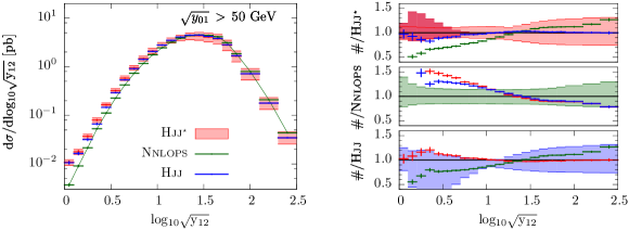
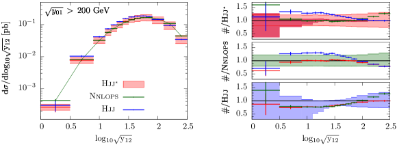
Figure 16: The $\log_{10}\sqrt{y_{12}}$ differential jet rates, defined according to the $k_{{\scriptscriptstyle\mathrm{T}}}$-jet algorithm with jet radius parameter $R=1$, and with cuts of $10$, $50$ and $200$ GeV imposed on $\sqrt{y_{01}}$.

The penultimate set of differential jet rates we wish to present are given in figure 16. Here we examine the key jet rate of interest to our studies, given its role in the proposed correction procedure, $\log_{10}\sqrt{y_{12}}$, but now subject to additional cuts in the $\sqrt{y_{01}}$ jet rate variable. These cuts are intended to bring to the fore events for which there is a hierarchy $y_{12}\ll y_{01}$ and associated large logarithm $L_{12}$. This aspect is indeed manifested in both $\log_{10}\sqrt{y_{12}}$ distributions in fig. 16 through the Sudakov peak shifting to higher $y_{12}$ values. The Sudakov peak in the inclusive distribution of fig. 14 is centred around $\log_{10}\sqrt{y_{12}}=1$ ($\sqrt{y_{12}}=10\textnormal{ }\mathrm{GeV}$), moving up to $\log_{10}\sqrt{y_{12}}\approx 1.5$ ($\sqrt{y_{12}}\approx 30\textnormal{ }\mathrm{GeV}$) on imposing the $\sqrt{y_{01}}>50\mbox{ }\mathrm{GeV}$ cut, as shown in the uppermost plot in fig. 16, and further to $\log_{10}\sqrt{y_{12}}\approx 1.75$ ($\sqrt{y_{12}}\approx 55\textnormal{ }\mathrm{GeV}$) on imposing the $\sqrt{y_{01}}>200\mbox{ }\mathrm{GeV}$ cut. The shifting of the peak to higher $y_{12}$ values is a manifestation of the fact that the cuts imply a proportionate increase in the available phase space for high $p_{{\scriptscriptstyle\mathrm{T}}}$ emission of the second pseudoparton.

One of the easiest features to make sense of in fig. 16, is the excess of the Nnlops results over $\textsc{Hjj}^{\star}$ and Hjj-Minlo predictions in the high $\sqrt{y_{12}}$ region, with the latter pair of results being indistinguishable there. This attribute is consistent with the enhancement of the Nnlops cross section over the corresponding Hjj-Minlo and $\textsc{Hjj}^{\star}$ results, in both the inclusive 2-jet cross section, with high jet $p_{{\scriptscriptstyle\mathrm{T}}}$ thresholds (fig. 3), and the transverse momentum spectrum of the second hardest jet (fig. 10). In the latter distribution the discrepancy increases with radiation hardness, as it does in fig. 16. Technically, the agreement of $\textsc{Hjj}^{\star}$ and Hjj-Minlo in this limit is also easy to understand, since in these regions $L_{12}$ is not large and the Minlo correction procedure ‘switches off’, with the Nnlops prediction being categorically inferior to Hjj-Minlo there. Specifically, the $h(L_{12})$ function (eq. 32) tends to zero.

Looking towards the Sudakov peak regions in fig. 16, where the great bulk of the cross section is centred, one expects, by virtue of the fact that our method is to return inclusive 0- and 1-jet Nnlops predictions, the Nnlops and $\textsc{Hjj}^{\star}$ predictions to agree well there. The results in figure 16 support this simple reasoning quite well.

Turning back to the 1-jet inclusive cross section predictions in fig. 3, with a 50 GeV jet $p_{{\scriptscriptstyle\mathrm{T}}}$ threshold, there is a relatively small difference between Hjj-Minlo and Nnlops predictions, this implies that, on average, the $\delta(\Phi_{{\scriptscriptstyle\mathcal{B}\mathrm{J}}})$ term in eq. 31 is very small in the context of that observable, which is in some reasonable degree of correspondence with the cumulant of the first distribution in figure 16 ($\sqrt{y_{01}}>50\mbox{ }\mathrm{GeV}$). Granted this point, it is then no surprise to observe that the $\textsc{Hjj}^{\star}$ and Hjj-Minlo predictions are essentially in perfect agreement all the way down to $\sqrt{y_{12}}\sim 3\mbox{ GeV}$, exhibiting only small differences beyond that point.

The difference in normalization of the Hjj-Minlo and Nnlops predictions in the case of the $\sqrt{y_{01}}>200\mbox{ }\mathrm{GeV}$ cut, can be anticipated by looking at the difference in the respective leading jet $p_{{\scriptscriptstyle\mathrm{T}}}$ spectra for $p_{{\scriptscriptstyle\mathrm{T}}}>200\mbox{ }\mathrm{GeV}$ (fig. 5), revealing a fairly flat 15% surplus of Hjj-Minlo over Nnlops. Indeed a 15% excess of Hjj-Minlo over Nnlops is what we also see here in the vicinity of the Sudakov peak, in the lower plot of fig. 16. In this region and that below, both dominated by large logarithmic corrections, one sees the improved $\textsc{Hjj}^{\star}$ result nicely following the Nnlops results.

Before leaving the discussion of figure 16 we must remark on the systematic uncertainty coming from the $\rho$ parameter (dark-red band). Indeed these observables have been mainly studied to try to expose and stress-test this aspect. The predictions of fig 16 show the biggest $\rho$ dependence of any in this paper. Sure enough, demanding that $\sqrt{y_{01}}$ be 50 or 200 GeV and then looking down at the $1\mbox{ GeV}\leq\sqrt{y_{12}}\leq 3\mbox{ GeV}$ (i.e. $0\leq\log_{10}\sqrt{y_{12}}\leq 0.5$) we see what looks like a sizable $\rho$ uncertainty. In the $\sqrt{y_{01}}>50\mbox{ }\mathrm{GeV}$ case we see this uncertainty rises up to ${}_{-20\%}^{+50\%}$ at $\sqrt{y_{12}}\approx 1.5\mbox{ GeV}$. In the same region of the $\sqrt{y_{01}}>200\mbox{ }\mathrm{GeV}$ distribution we see an uncertainty similar in magnitude, however, for this plot the conclusion is less precise, due to the appearance of large statistical uncertainties. Taking together the following points, we believe we can now conclude that the uncertainty due to our $\rho$ parameter is in general negligible: i.) we took a rather conservative approach to assessing the uncertainty due to $\rho$, varying it from 1 to $27$, ii.) we constructed observables to isolate and expose potential problems owing to $\rho$, we found no pathologies, and the latter uncertainty only showed up in the very deep Sudakov region, where theoretical control is very limited.

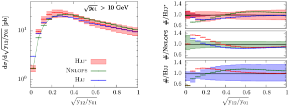
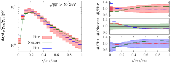
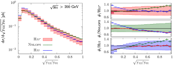
Figure 17: Ratios of differential jet rates, $\sqrt{y_{12}/y_{01}}$, defined according to the $k_{{\scriptscriptstyle\mathrm{T}}}$-jet algorithm with jet radius parameter $R=1$, and with cuts of $10$, $50$ and $200$ GeV imposed on $\sqrt{y_{01}}$.

We conclude the presentation of results on jet rates with the $\sqrt{y_{12}/y_{01}}$ distributions in fig. 17. The latter quantity is precisely that which our Minlo improvement procedure directly modifies, in order to achieve agreement with the inclusive $\Phi_{{\scriptscriptstyle\mathcal{B}\mathrm{J}}}$ distribution of the Nnlops (see again sects. 2.6 and 3). The three $\sqrt{y_{12}/y_{01}}$ plots in fig. 17 are also in rough correspondence with those for $\log_{10}\sqrt{y_{12}}$ in figs. 14 and 16. Indeed, the arrangement of the three predictions relative to one another in fig. 16, for the $\sqrt{y_{01}}>50\mbox{ GeV}$ and $\sqrt{y_{01}}>200\mbox{ GeV}$ cuts, is essentially the same as that which one finds for the same $\sqrt{y_{01}}$ cuts applied to the $\sqrt{y_{12}/y_{01}}$ distribution in fig. 17. This correspondence is to expected, if one assumes that the bulk of events making the distributions in both cases ($\log_{10}\sqrt{y_{12}}$ and $\sqrt{y_{12}/y_{01}}$) is dominated by those having $\sqrt{y_{01}}$ close to the cut; this assumption is reasonably fair, given that $\sqrt{y_{01}}$ falls off quickly, like the leading jet $p_{{\scriptscriptstyle\mathrm{T}}}$ spectrum. Crudely speaking, this makes the denominator of $\sqrt{y_{12}/y_{01}}$ a constant and, by implication, $\sqrt{y_{12}/y_{01}}$ tends to look the same as scaled a plot of $\sqrt{y_{12}}$. We also consider that the $\sqrt{y_{12}/y_{01}}$ distribution for $\sqrt{y_{01}}>10\mbox{ GeV}$ bears a considerable resemblance to that of the inclusive $\log_{10}\sqrt{y_{12}}$ one in fig. 14. This makes sense on the basis that the $\sqrt{y_{01}}$ cut on the former distribution is loose to the point of being no cut at all. This being the case, we refer back to our discussion on the features of the aforementioned $\log_{10}\sqrt{y_{12}}$ plots, for explanation of the structures in the $\sqrt{y_{12}/y_{01}}$ ones.

Higgs-jet and dijet correlations

In this subsection we move to check observables more sensitive directional correlations between the Higgs boson and jets in the event. Such variables are routinely encountered in experimental analysis relating to Higgs production via vector boson fusion. In leaving the jet rate variables behind, we return again to define all jets according to the anti-$k_{t}$ clustering algorithm with radius parameter $R=0.4$, for all of the remaining numerical results in this work.

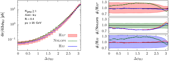
Figure 18: Azimuthal angle between the Higgs boson and leading jet, with jets defined according to the anti-$k_{t}$ algorithm with a $25$ GeV transverse momentum threshold and radius parameter $R=0.4$.

We start with the azimuthal separation of the Higgs boson and the leading jet, $\Delta\phi_{{\scriptscriptstyle\mathrm{HJ}}}$, for events containing at least one jet, in fig. 18. The region $\Delta\phi_{{\scriptscriptstyle\mathrm{HJ}}}\approx\pi$ is dominated by configurations consisting of a hard underlying Higgs-plus-one jet configuration, accompanied by additional soft radiations. Decreasing $\Delta\phi_{{\scriptscriptstyle\mathrm{HJ}}}$ implies an increased amount of radiation beyond that in the hard underlying Higgs-plus-one jet configuration (to balance momentum in the transverse plane). Indeed, if we assume that this extra radiation is collimated into a single would-be jet, then already in the vicinity of $\Delta\phi_{{\scriptscriptstyle\mathrm{HJ}}}\approx 2.1$ the distribution is becoming dominated by Mercedes-star configurations of the Higgs, jet and the would-be jet, as well as others involving yet greater angular separation of the leading jet and would-be jet. Bearing in mind the latter point, the near perfect agreement of the Hjj-Minlo and $\textsc{Hjj}^{\star}$ predictions for $\Delta\phi_{{\scriptscriptstyle\mathrm{HJ}}}\lesssim 2.1$ is expected and desired; both being NLO accurate in the description of 2-jet observables. In the region $\Delta\phi_{{\scriptscriptstyle\mathrm{HJ}}}>2.1$ we see the $\textsc{Hjj}^{\star}$ result gently lifts off the Hjj-Minlo one. This lift-off is qualitatively expected, on the basis that the integral of this distribution must equal the inclusive 1-jet cross section, with a 25 GeV jet transverse momentum cut, and we know that the inclusive 1-jet cross section from $\textsc{Hjj}^{\star}$ (and to a lesser extent Nnlops) exhibits a 5% enhancement over that of Hjj-Minlo (see again fig. 3).

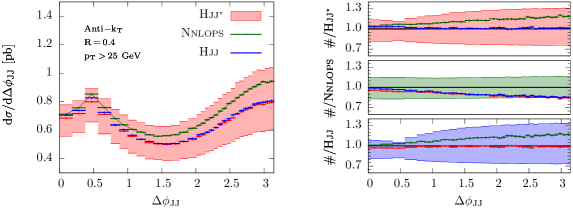
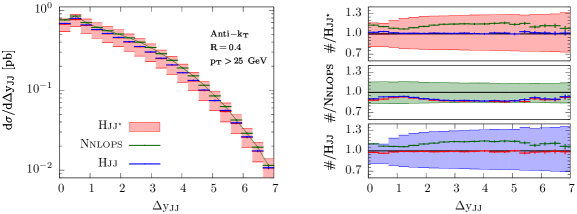
Figure 19: Azimuthal (top) and rapidity (bottom) separation between the two leading jets, with jets defined according to the anti-$k_{t}$ algorithm with a $25$ GeV transverse momentum threshold and radius parameter $R=0.4$.

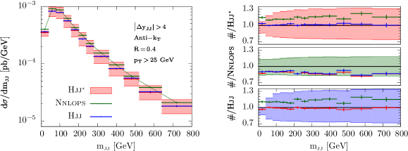
Figure 20: In this plot we show the invariant mass of the two leading jets, for events in which they have a rapidity separation greater than four. The jets have been defined according to the anti-$k_{t}$ clustering algorithm, with radius parameter $R=0.4$, and with a transverse momentum threshold of 25 GeV.

In figure 19 we display the azimuthal separation of the two leading jets in the uppermost plot and their rapidity separation in the lower one. In figure 20 we have further plotted the invariant mass of the two leading jets, for events in which they are separated by at least four units of rapidity. All of these distributions demand the presence of at least two jets in the final state. From the analysis of our foregoing results, we understand that for a global jet $p_{{\scriptscriptstyle\mathrm{T}}}$ threshold of 25 GeV, we can expect that 2-jet inclusive observables, such as these, are dominated by events with no strong hierarchy of scales $y_{12}\ll y_{01}$. Consequently, we expect, and we find, that our corrective procedure has no effect, with the $\textsc{Hjj}^{\star}$ and Hjj-Minlo results being indistinguishable from one another throughout. This is again our desired behaviour given that the Hjj-Minlo prediction is nominally NLO accurate for these observables, while the Nnlops is similarly just LO. Lastly, we add that the same conclusions hold for the $m_{{\scriptscriptstyle\mathrm{JJ}}}$ distribution when the $\left|\Delta\mathrm{y}_{{\scriptscriptstyle\mathrm{JJ}}}\right|>4$ rapidity separation cut is not imposed, in particular, the $\textsc{Hjj}^{\star}$ and Hjj-Minlo results remain indistinguishable, with the Nnlops continuing to exhibit the same relative discrepancy (albeit within a smaller scale uncertainty band).

Jet binned Higgs boson transverse momentum distribution

The final results we present, in figs. 21-22, are of the Higgs boson transverse momentum spectrum, in events with a given exclusive jet multiplicity. The jets in question were defined according to the anti-$k_{t}$ jet algorithm with $R=0.4$ and a jet transverse momentum threshold of 30 GeV.

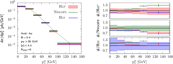
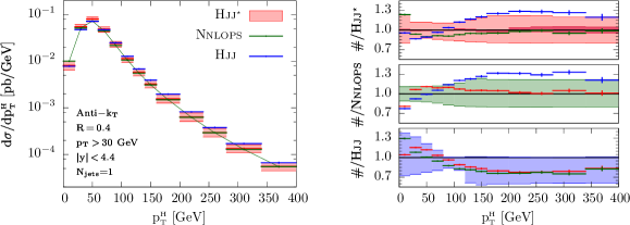
Figure 21: In the upper plot we show the transverse momentum distribution of the Higgs boson in 0-jet events. Jets are here constructed according to the anti-$k_{t}$ clustering algorithm, for a radius parameter $R=0.4$. Jets are required to have transverse momentum $p_{{\scriptscriptstyle\mathrm{T}}}\geq 30$ GeV and rapidity $\left|\mathrm{y}\right|\leq 4.4$. The corresponding distribution in the case of 1-jet events is shown below.

Figure 21 shows the Higgs boson’s transverse momentum in 0-jet events in the upper plot and in 1-jet events in the lower one. In the case of the 0-jet events we see the $\textsc{Hjj}^{\star}$ prediction aligns itself with the superior (NNLO) Nnlops result in the low transverse momentum domain. On the other hand, as soon as the Higgs boson has reaches a transverse momentum in excess of that of the jet defining $p_{{\scriptscriptstyle\mathrm{T}}}$ threshold, we see that $\textsc{Hjj}^{\star}$ quickly comes into agreement with Hjj-Minlo. This behaviour is also as intended, since in the latter region, momentum conservation combined with the requirement that there be no resolved jets, dictates that the Higgs boson must be considered as recoiling against multiple hard radiations which are widely separated in angle from one another, all with $p_{{\scriptscriptstyle\mathrm{T}}}<30\mbox{ {GeV}}$. The latter class of ‘hedgehog’ configurations is described more accurately by the higher multiplicity Hjj-Minlo simulation.

Turning to the Higgs transverse momentum in the 1-jet events, we see the results we naively expect in the region $p_{{\scriptscriptstyle\mathrm{T}}}^{{\scriptscriptstyle\mathrm{H}}}>100\text{ GeV}$, with Nnlops and $\textsc{Hjj}^{\star}$ in very good agreement. In the region surrounding the peak of the distribution at $p_{{\scriptscriptstyle\mathrm{T}}}^{{\scriptscriptstyle\mathrm{H}}}\sim 50\text{ GeV}$, $\textsc{Hjj}^{\star}$ continues to agree well with Hjj-Minlo, but not quite as nicely as before. The slight excess of the $\textsc{Hjj}^{\star}$ prediction over the Nnlops around this peak follows the same explanation as for the similarly sized enhancement of the exclusive 1-jet cross section of the former over the latter, in the discussion surrounding fig. 4. There we explained that our correction procedure led to an enhanced 1-jet exclusive cross section, by acting to recover the inclusive 1-jet cross section of the Nnlops, while maintaining the 2-jet inclusive cross section of Hjj-Minlo; since the 2-jet inclusive cross section of Hjj-Minlo was low with respect to that of the Nnlops, the $\textsc{Hjj}^{\star}$ 1-jet exclusive cross section therefore had to be high. Remarkably, on the other hand, we note that for the lowest bin in the $\mathrm{N_{jets}}=1$ $p_{{\scriptscriptstyle\mathrm{T}}}^{{\scriptscriptstyle\mathrm{H}}}$ plot, it is in fact natural and correct that the $\textsc{Hjj}^{\star}$ distribution is found to be in complete agreement with Hjj-Minlo, for in that region the recoil of the leading jet can no longer be balanced by the Higgs boson, and instead extra radiation must be present to this end.

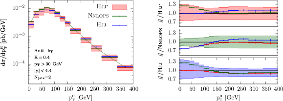
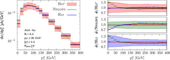
Figure 22: In the upper plot we show the transverse momentum distribution of the Higgs boson in 2-jet events. Jets are here constructed according to the anti-$k_{t}$ clustering algorithm, for a radius parameter $R=0.4$. Jets are required to have transverse momentum $p_{{\scriptscriptstyle\mathrm{T}}}\geq 30$ GeV and rapidity $\left|\mathrm{y}\right|\leq 4.4$. The corresponding distribution in the case of $\geq 3$-jet events is shown underneath.

Lastly, we look to the Higgs boson transverse momentum distributions in the exclusive 2-jet events and inclusive 3-jet events, in the upper and lower plots of fig. 22. For both the exclusive 2-jet and inclusive 3-jet $p_{{\scriptscriptstyle\mathrm{T}}}^{{\scriptscriptstyle\mathrm{H}}}$ spectra, we see that $\textsc{Hjj}^{\star}$ agrees perfectly with the Hjj-Minlo generator in the low transverse momentum domain. In the high transverse momentum regions we find that all three predictions agree rather well with one another. In the exclusive 2-jet case at high $p_{{\scriptscriptstyle\mathrm{T}}}^{{\scriptscriptstyle\mathrm{H}}}$, we can, however, clearly see that the correction procedure has driven $\textsc{Hjj}^{\star}$ to reproduce Nnlops rather than Hjj-Minlo. We believe that this too is again the desired result and that the Nnlops prediction is superior to that of Hjj-Minlo in this particular kinematic domain. This assumption is based on the fact that in high $p_{{\scriptscriptstyle\mathrm{T}}}^{{\scriptscriptstyle\mathrm{H}}}$ $\mathrm{N}_{\mathrm{jets}}=2$ events, the leading jet has a transverse momentum which is bounded from below by approximately half that of the Higgs boson, moreover, it will tend to have a transverse momentum close to that of the Higgs. Thus, the $p_{{\scriptscriptstyle\mathrm{T}}}^{{\scriptscriptstyle\mathrm{H}}}\sim\mathrm{200}\text{ GeV}$ region of the $\mathrm{N}_{\mathrm{jets}}=2$ events $p_{{\scriptscriptstyle\mathrm{T}}}^{{\scriptscriptstyle\mathrm{H}}}$ spectrum, will be dominated by events with $\sqrt{y_{01}}\sim 200\mbox{ GeV}$. Referring back to the $\log_{10}\sqrt{y_{12}}$ plot of fig. 16, with the $\sqrt{y_{01}}>200\text{ GeV}$ cut imposed, we can then understand that nearly all such events will come with a second $p_{{\scriptscriptstyle\mathrm{T}}}>30\mbox{ GeV}$ jet ‘for free’, i.e. the $p_{{\scriptscriptstyle\mathrm{T}}}^{{\scriptscriptstyle\mathrm{H}}}$ spectrum with $\mathrm{N}_{\mathrm{jets}}=2$, for $p_{{\scriptscriptstyle\mathrm{T}}}^{{\scriptscriptstyle\mathrm{H}}}\gtrsim\mathrm{200}\text{ GeV}$, becomes essentially the $\mathrm{N}_{\mathrm{jets}}\geq 1$ $p_{{\scriptscriptstyle\mathrm{T}}}^{{\scriptscriptstyle\mathrm{H}}}$ distribution. Hence, we believe the Nnlops/$\textsc{Hjj}^{\star}$ prediction to be more accurate than Hjj-Minlo in this case.

5 Conclusion

In this work we have revisited the Minlo and Minlo^′ frameworks. Our main aim has been to address the issue of how to extend the accuracy of existing Minlo simulations up to that of Minlo^′. We focused on Minlo simulations of $\mathcal{B}$+2-jet production ($\mathcal{B}\textsc{jj}$), with $\mathcal{B}$ a colourless system, as prototypical ‘complex processes’, however, our ideas are more widely applicable. For the latter generators, which are NLO accurate in the description of $\mathcal{B}$+2-jet ($\mathcal{B}\textsc{jj}$) inclusive observables, promotion to Minlo^′ accuracy amounts to the requirement that $\mathcal{B}$+1-jet ($\mathcal{B}\textsc{j}$) inclusive quantities also be recovered at NLO. We have also considered how to go further in this framework, and obtain (N)NLO accuracy for inclusive $\mathcal{B}$-production observables from $\mathcal{B}\textsc{jj}$-Minlo.

In existing Minlo^′ simulations the two-fold NLO accuracy is obtained by constructing a Sudakov form factor which returns the relevant inclusive NLO $\mathcal{B}m\textsc{j}$ cross sections, differential in the underlying Born phase space, starting from NLO $\mathcal{B}n\textsc{j}$ cross sections, with $m=n-1$. While the form factors are explicitly constructed from high-order resummation ingredients, the accuracy of the resummation in the resulting Minlo^′ simulation is the same as in the initial Minlo one. The net effect of the modifications is to carefully unitarize the inclusive cross section, differential in the Born kinematics. This is very similar to the working of Powheg Sudakov form factors in Nlops matching. The latter contain NLL and even power suppressed terms in the exponent in order to recover NLO accuracy, despite being, in general, just LL accurate.

We started in this work by trying to clarify to what extent the $\mathcal{B}\textsc{jj}$-Minlo simulations already achieve the aforementioned Minlo^′ accuracy, and to see how to improve them in this direction by better understanding the relevant resummation. We used the Caesar formalism to derive a $\mathrm{NNLL}_{\sigma}$ resummation formula for the $0\rightarrow 1$-$k_{t}$-jet rate $y_{01}$ and, separately, the $1\rightarrow 2$ jet rate $y_{12}$; including leading multiple emission corrections in the exclusive $k_{t}$-algorithm. The $\mathrm{NNLL}_{\sigma}$ formula reveals existing $\mathcal{B}\textsc{jj}$-Minlo simulations miss $\mathrm{NLL}_{\sigma}$ terms in their $y_{12}$ Sudakov form factor exponents, associated to soft-wide angle gluon emission from the underlying $\mathcal{B}\textsc{j}$ state in the kinematic domain where Caesar is valid, $y_{01}\gtrsim m_{{\scriptscriptstyle\mathrm{H}}}^{2}$. The Sudakov form factors in existing $\mathcal{B}\textsc{jj}$-Minlo codes also miss the $\mathrm{NNLL}_{\sigma}$ multiple emission corrections in the resummation formula. With these clarifications one could formally improve $\mathcal{B}\textsc{jj}$-Minlo codes towards $\mathcal{B}\textsc{jj}$-Minlo^′, implementing improved Sudakov form factors to that end.

We derived the fixed order expansion of the $\mathrm{NNLL}_{\sigma}$ Caesar formula and from this we showed how our Minlo procedure applied to the $\mathcal{B}$j(j) NLO computations returns a matched, resummed, NLO accurate jet resolution spectrum. In doing so we also assumed the presence of unknown $\mathrm{N^{3}LL}_{\sigma}$ and $\mathrm{NNLL}_{\sigma}$ terms in our initial fixed order expansion formula; the former owe to the limitations of our initial resummation formula truncated at NLO, while we allowed for the presence of the latter in anticipation of a breakdown of the Caesar framework in considering the region $y_{01}\ll m_{{\scriptscriptstyle\mathrm{H}}}^{2}$ later on. Upon integration over the Minlo jet resolution spectrum, we determine how the distribution of the Born kinematics differs from that of conventional NLO on account of those unknown terms, which were tracked and contained. We demonstrate how such unwanted terms are removed in the original Minlo^′ approach and, based on that, we introduced an approximately equivalent procedure, which promotes the Minlo simulations to Minlo^′ accuracy without the need of analytic expressions for higher order terms in the Sudakov form factor — terms which are in general unknown. To this end we solve the condition that the missing higher order Sudakov contribution must be such that $\mathcal{B}m$j-Minlo recover the (N)NLO results for $\mathcal{B}n$j Born kinematics, when suitably integrated, to determine a numerical approximation to the former. The Sudakov correction so-derived renders $\mathcal{B}m$j-Minlo (N)NLO accurate for $\mathcal{B}n$j inclusive observables, while maintaining NLO accuracy for $\mathcal{B}m$j ones.

This procedure is a useful extension of the Minlo framework. Despite the fact that Minlo^′ is proven to recover conventional NLO results for inclusive quantities up to NNLO ambiguities, in the original Minlo^′ paper modest numerical disagreements were found, between the predictions of $\mathcal{B}\textsc{j}$-Minlo^′ and conventional NLO, for W and Z production. With the suggested extension of the Minlo method in this paper, by construction, the predictions for fully inclusive observables become essentially identical to the standard NLO predictions.

A more important benefit of the proposed extension is that one can begin to make Minlo^′ simulations, merging two units of multiplicity at NLO, or one NLO and one NNLO, without a merging scale, for complex processes, provided the resummation in the Minlo program entering the correction procedure is $\mathrm{NLL}_{\sigma}$ accurate. The main limitation to be faced in practice will occur for processes in which the dimensionality of the underlying Born phase space is high; in this case the numerical determination of the $\delta\left(\Phi\right)$ term (eq. 31) which corrects the Sudakov form factor will become challenging. We should be clear though that, broadly speaking, the main objective in this work has been to demonstrate that one can use precision inclusive cross sections to determine approximate corrections to the Sudakov form factor of Minlo simulations, such that they return the correct (N)NLO Born kinematics; this in turn leads to (N)NLO accuracy for arbitrary infrared-safe observables which nominally receive their leading contributions from parton multiplicities lower than that included in the initial Minlo simulation. The precise way we have done this, discussed in the second part of section 2.6, and our implementation of it, is undoubtedly just one option out of many, and can be simply considered as a practical, working, proof-of-concept at this point. Even in the worst case, should the dimensionality of the Born kinematics become too much, the method here still has the potential to greatly improve results, in approximating the full $\delta\left(\Phi\right)$ term of eq. 31 by a carefully dimensionally reduced version of it.

The loose requirement on the accuracy of the Minlo resummation has an additional useful property: the method can be applied in regions of phase-space where the underlying Born itself has disparate kinematic scales associated with it; in such regions achieving high accuracy resummation is currently a formidable challenge. In particular, our improvement procedure remains valid for $\mathcal{B}\textsc{jj}$-Minlo in regions of phase-space where $y_{01}$ is much smaller than $m_{{\scriptscriptstyle\mathcal{B}}}^{2}$, where both large logarithms of $m_{{\scriptscriptstyle\mathcal{B}}}^{2}/y_{01}$ and $y_{01}/y_{12}$ require resummation. To this end we first argued that the Caesar $y_{01}/y_{12}$ resummation remains $\mathrm{NLL}_{\sigma}$ accurate in the region $y_{01}\ll m_{{\scriptscriptstyle\mathcal{B}}}^{2}$. Our argument is largely based on the finding that the Caesar Sudakov form factor for this variable is the same as that prescribed by the coherent branching formalism at $\mathrm{NLL}_{\sigma}$ (except for a subset of the soft-wide-angle radiation, which is beyond the accuracy of the latter). We also note that the leading $\mathrm{NLL}_{\sigma}$ terms in the fixed order expansion of the Caesar resummation formula are obtained by integrating a single soft/collinear emission over the region $y_{12}<y_{01}$, i.e. they are the same whether $y_{01}\ll m_{{\scriptscriptstyle\mathcal{B}}}^{2}$, or not. Taking the latter two points together, it follows that the Caesar $y_{01}/y_{12}$ resummation must hold at the $\mathrm{NLL}_{\sigma}$ level, even in the difficult regions.

The fact that $y_{12}$ resummation works in all regions of phase-space implies one can do a ‘nested’ Minlo^′ simulation with the help of our proposed extension: instead of using unitarity such that partially integrated $\mathcal{B}\textsc{jj}$ distributions become equal to the NLO $\mathcal{B}\textsc{j}$ distributions, we train them on Minlo^′ $\mathcal{B}\textsc{j}$ distributions. This makes them also NLO correct in inclusive $\mathcal{B}$ distributions, since the latter are obtained on suitably integrating over radiation in $\mathcal{B}\textsc{j}$-Minlo^′. In this way the extension of the Minlo^′ method to the merging of more than two multiplicities is realised.

As a feasibility study for the latter, we have applied our correction procedure to Hjj-Minlo. We start from a LHE event file for the Hjj-Minlo simulation and reweight the events such that distributions differential in $\Phi_{{\scriptscriptstyle\mathrm{HJ}}}$ become equal to the existing NNLO-improved Hj-Minlo^′ calculation, without hampering the formal accuracy of the Hjj-Minlo simulation. We therefore made predictions that are NNLO accurate for inclusive Higgs boson production, and NLO accurate for Hj and Hjj observables. Since the LHE events are ultimately generated according to the Powheg Nlops matching procedure they may, of course, be showered in the usual way. Our numerical results are very encouraging: for inclusive observables in H and Hj production, we recover the results of the Hnnlops simulation, while for observables in which $y_{12}\sim y_{01}$ we recover the Hjj-Minlo predictions, with smooth interpolation between them.

There is ample freedom in the functional form of the reweighting factor which is formally beyond the accuracy of the method. We have explored (some of) its dependence and seen essentially no visible effects of it in the many distributions we have examined. The distribution which displayed most sensitivity to this ambiguity was, unsurprisingly, $\log_{10}\sqrt{y_{12}}$. Even for this variable, the sensitivity is located in the deep Sudakov region, mostly well-below the Sudakov peak, a region which is anyway very sensitive to higher order resummation and non-perturbative effects.

There are a number of aspects of this work which can be explored further and refined. It is clear, for example, that it is interesting to consider our approach in application to other processes. We have shown the method can work well for a process with 3 final-state particles (Hjj), thus it seems reasonable to expect similar quality results in application to processes with equal multiplicity, e.g. trijet, and jet-associated single-top/top-pair production (with some approximation in the handling of top decays). In fact these processes are in one sense less demanding than that which we demonstrated, in so far as we dealt with a process for which two jets could become unresolved, moreover, this was handled while mapping onto an NNLO calculation of Higgs production. On the other hand, for high multiplicity processes like VBF Higgs-plus-3-jet production, the dimensionality of the phase space combined with the problems to be anticipated in obtaining high statistics for determining $\delta\left(\Phi\right)$, would likely prove too cumbersome in practice, at least for our proof-of-concept implementation. Nevertheless, in the absence of a better alternative, we would still advocate trying the latter method in some approximate form, e.g. applying it on only a carefully selected subset of the variables which parametrize the underlying Born kinematics. Depending on the initial circumstances this may lead to very desirable improvements.

Relatedly, on a technical level it is worth considering a more sophisticated approach to our implementation, e.g. using an adaptive, optimised, grid parametrization procedure for the underlying Born phase space, together with advanced interpolation procedures for computing $\delta\left(\Phi\right)$. Having said that, it is perhaps a good indicator of the potential of this approach, that it appears to have worked remarkably well even with just a basic implementation using hand-made rigid grids. From a theoretical perspective, one may wish to consider improvements to the $\mathcal{B}\textsc{jj}$-Minlo^′ codes based on our comparison of their inherent resummation and that of the Caesar framework, such as inclusion of soft-wide-angle ($\Delta S_{1}$) and multiple emission ($\mathcal{F}_{2}$) terms in the Sudakov form factors. Our numerical studies in this paper suggest that these inclusions would be of really quite limited interest though.

A further investigation would be to consider the effect of breaking the reweighting procedure for $\mathcal{B}\textsc{jj}$-Minlo into two phases: in the first stage just the inclusive $\Phi_{{\scriptscriptstyle\mathcal{B}}}$ distribution of $\mathcal{B}\textsc{jj}$-Minlo is corrected to that of $\mathcal{B}\textsc{j}$-Minlo^′, by adjusting the $y_{01}$ distribution; in the second stage the procedure is applied to the $\mathcal{B}\textsc{jj}$-Minlo output from the first stage, in exactly the same way as set out in sects. 3-4. At the $\mathrm{NLL}_{\sigma}$ level, there is no distinguishing between the latter approach and that which we carried out. On the other hand, it is clear that, at some level, the effective Sudakov form factor correction that we derive for the $y_{01}/y_{12}$ resummation will make up for what might better be considered as deficiencies in the $y_{01}$ Sudakov form factor. Nevertheless, from our numerical studies here, we expect that this change would only register much like the $\rho$-parameter variations that we assessed, i.e. we believe it will only become visible in $y_{12}$ regions which are under poor theoretical control (the deep Sudakov region). It is also important not to over emphasise this point in view of the fact that the correction procedure obtains the $\Phi_{{\scriptscriptstyle\mathcal{B}}}$, $y_{01}$ and $\mathrm{y}_{{\scriptscriptstyle\mathrm{J}}}$ distributions of $\mathcal{B}\textsc{j}$-Minlo^′, by construction, in any case. Nevertheless, this alternative may prove advantageous in other applications of the method.

Appendix A Appendix

A.1 Derivation of $\mathrm{LL}$/$\mathrm{NNLL}_{\sigma}$ jet resolution spectra

In this appendix we give details on how our general $\mathrm{NNLL}_{\sigma}$ jet resolution spectrum is arrived at from the results of refs. Banfi:2004yd and Banfi:2010xy .

In eqs. 3.14-3.17 of ref. Banfi:2010xy the $\mathrm{NLL}$ resummed cumulant cross section, matched to NLO, to yield also $\mathrm{NNLL}_{\sigma}$ accuracy is given as

$$\frac{d\Sigma_{{\scriptscriptstyle\mathcal{R}}}\left(L\right)}{d\Phi}=\frac{d\sigma_{0}}{d\Phi}\,\left(1+\alpha_{{\scriptscriptstyle\mathrm{S}}}C_{1}\right)\,f\left(v\right)\,,$$ (50)

with $d\sigma_{0}/d\Phi$ the leading order cross section fully differential in the Born kinematics (denoted $\mathcal{B}$ in Banfi:2004yd ; Banfi:2010xy ), and with $f\left(v\right)$ encoding the resummation. The term $\alpha_{{\scriptscriptstyle\mathrm{S}}}C_{1}$ is the matching coefficient defined by (eq. 3.16 of ref. Banfi:2010xy )

$$\alpha_{{\scriptscriptstyle\mathrm{S}}}C_{1}=\lim_{L\rightarrow\infty}\,\left(\frac{d\Sigma_{{\scriptscriptstyle\mathrm{NLO}}}\left(L\right)}{d\Phi}-\left.\frac{d\Sigma_{{\scriptscriptstyle\mathcal{R},1}}\left(L\right)}{d\Phi}\right|_{{\scriptscriptstyle\bar{\chi}_{1}\rightarrow 0}}\right)\,/\,\frac{d\sigma_{0}}{d\Phi}\,,$$ (51)

where the $d\Sigma_{{\scriptscriptstyle\mathrm{NLO}}}\left(L\right)$ in our notation corresponds to $d\Sigma_{1}\left(v\right)$ of Banfi:2010xy , and with our $d\Sigma_{{\scriptscriptstyle\mathcal{R},1}}\left(L\right)$ corresponding to $d\Sigma_{r,1}\left(v\right)$ of Banfi:2010xy . Thus the matching coefficient of Banfi:2010xy is in our notation $\alpha_{{\scriptscriptstyle\mathrm{S}}}C_{1}=\bar{\alpha}_{{\scriptscriptstyle\mathrm{S}}}\bar{\chi}_{1}\left(\Phi\right)$. The function $f\left(v\right)$ is the main result of ref. Banfi:2004yd (see eq. 3.6 therein) and is comprised as follows (taking $b_{\ell}=0$, $a_{\ell}=2$, $d_{\ell}=g_{\ell}=1$, and hence $\bar{d}_{\ell}=1$, as appropriate for the $k_{t}$-jet resolution variables considered in our work, namely, $V\left(\left\{\tilde{p}\right\},k\right)=(k_{t}^{\left(\ell\right)}/Q)^{2}$):

$$f\left(v\right) = \mathcal{F}\left(R^{\prime}\right)\,S\left(T\left(\frac{L}{2}\right)\right)\,\exp\left[-\sum_{\ell=1}^{n}\,\left[C_{\ell}r_{\ell}\left(L\right)+B_{\ell}C_{\ell}T\left(\frac{L}{2}\right)\right]\right]\,\prod_{\ell=1}^{n_{i}}\,\frac{q^{\left(\ell\right)}\left(x_{\ell},\mu_{{\scriptscriptstyle F}}^{2}v\right)}{q^{\left(\ell\right)}\left(x_{\ell},\mu_{{\scriptscriptstyle F}}^{2}\right)}.$$ (52)

In ref. Banfi:2004yd , between eqs. A 1.18 and A 1.19, it is stated that for processes with less than four colour-charged legs in the hard underlying Born kinematics, $S\left(t\right)=\exp\left[S_{1}t\right]$, with $S_{1}$ as given in our eqs. 7, 2.2.

From ref. Banfi:2004yd eqs. 2.21-2.22, (taking $b_{\ell}=0$, $a_{\ell}=2$, $d_{\ell}=g_{\ell}=1$, and hence $\bar{d}_{\ell}=1$), we also have

$$r_{\ell}\left(L\right)=\int_{y}^{Q^{2}}\,\frac{dk_{t}^{2}}{k_{t}^{2}}\,\bar{\alpha}_{{\scriptscriptstyle\mathrm{S,CMW}}}\left(k_{t}^{2}\right)\,\ln\frac{Q^{2}}{k_{t}^{2}}\,,\qquad\mbox{and}\qquad T\left(\frac{L}{2}\right)=\int_{y}^{Q^{2}}\,\frac{dk_{t}^{2}}{k_{t}^{2}}\,2\bar{\alpha}_{{\scriptscriptstyle\mathrm{S}}}\left(k_{t}^{2}\right)\,,$$ (53)

where $\bar{\alpha}_{{\scriptscriptstyle\mathrm{S,CMW}}}$ is the so-called Bremsstrahlung (CMW) scheme for the strong coupling constant (as written on pg. 17 in Banfi:2004yd )

$$\bar{\alpha}_{{\scriptscriptstyle\mathrm{S,CMW}}}=\bar{\alpha}_{{\scriptscriptstyle\mathrm{S,\overline{MS}}}}+K\bar{\alpha}_{{\scriptscriptstyle\mathrm{S}}}^{2}\,.$$ (54)

Inserting the expressions for $\bar{\alpha}_{{\scriptscriptstyle\mathrm{S,CMW}}}$, $r_{\ell}\left(L\right)$, $T\left(\frac{L}{2}\right)$, $S\left(T\left(\frac{L}{2}\right)\right)$ into that for $f\left(v\right)$ gives, with no approximations,

$$f\left(v\right) = \mathcal{F}\left(R^{\prime}\right)\,\exp\left[-\int_{0}^{L}\,dL^{\prime}\,\bar{\alpha}_{{\scriptscriptstyle\mathrm{S}}}^{2}\left(y^{\prime}\right)\,2G_{12}\,\left[\,4\mathcal{F}_{2}G_{12}\,\right]L^{\prime}\right]\,\left[\exp\left[-R\left(v\right)\right]\,\prod_{\ell=1}^{n_{i}}\,\frac{q^{\left(\ell\right)}\left(x_{\ell},\mu_{{\scriptscriptstyle F}}^{2}v\right)}{q^{\left(\ell\right)}\left(x_{\ell},\mu_{{\scriptscriptstyle F}}^{2}\right)}\right]\,.$$ (55)

with $-R\left(v\right)$ here as given in our eq. 4.

Now we start to make approximations and deviate from ref. Banfi:2004yd , breaking the NLL resummation by $\mathrm{N^{3}LL_{\sigma}}$ terms. Consider that $\mathcal{F}\left(R^{\prime}\right)$ resums single log terms as

$$\mathcal{F}\left(R^{\prime}\right)=1+\mathcal{F}_{2}R^{\prime 2}+...+\mathcal{O}\left(\mathcal{F}_{n}R^{\prime n}\right)+...\,,$$ (56)

$R^{\prime}=\partial_{L}R\left(v\right)$ and so $R^{\prime n}$ is $\mathcal{O}\left(\bar{\alpha}_{{\scriptscriptstyle\mathrm{S}}}^{n}L^{n}\right)$. Neglecting terms of $\mathrm{N^{3}LL_{\sigma}}$ accuracy we can simply replace $R^{\prime}=\bar{\alpha}_{{\scriptscriptstyle\mathrm{S}}}\left(y\right)\,2G_{12}\,L$

$$\mathcal{F}\left(R^{\prime}\right) = \exp\left[\,\int_{0}^{L}dL^{\prime}\,\bar{\alpha}_{{\scriptscriptstyle\mathrm{S}}}^{2}\left(y\right)\,2G_{12}\,\left[\,4\mathcal{F}_{2}G_{12}\,\right]\,L^{\prime}\right]\,,$$ (57)

and hence

$$f\left(v\right) = \exp\left[-R\left(v\right)\right]\,\prod_{\ell=1}^{n_{i}}\,\frac{q^{\left(\ell\right)}\left(x_{\ell},\mu_{{\scriptscriptstyle F}}^{2}v\right)}{q^{\left(\ell\right)}\left(x_{\ell},\mu_{{\scriptscriptstyle F}}^{2}\right)}\,+\,\mathcal{O}\left(\mathrm{N^{3}LL}_{\sigma}\right).$$ (58)

We then have the $\mathrm{LL}$/$\mathrm{NNLL}_{\sigma}$ resummed cumulant expression

$$\frac{d\Sigma_{{\scriptscriptstyle\mathcal{R}}}\left(L\right)}{d\Phi}=\frac{d\sigma_{0}}{d\Phi}\,\left(1+\bar{\alpha}_{{\scriptscriptstyle\mathrm{S}}}\left(\mu_{{\scriptscriptstyle R}}^{2}\right)\bar{\chi}_{1}\left(\Phi\right)\right)\,\left[\exp\left[-R\left(v\right)\right]\,\prod_{\ell=1}^{n_{i}}\,\frac{q^{\left(\ell\right)}\left(x_{\ell},\mu_{{\scriptscriptstyle F}}^{2}v\right)}{q^{\left(\ell\right)}\left(x_{\ell},\mu_{{\scriptscriptstyle F}}^{2}\right)}\right]\,.$$ (59)

Recall that $\bar{\chi}_{1}$ encodes hard-virtual and hard-collinear splitting corrections, and that these contributions contain terms which cancel the $\mu_{{\scriptscriptstyle R}}$ and $\mu_{{\scriptscriptstyle F}}$ dependence of $d\sigma_{0}/d\Phi_{{\scriptscriptstyle\mathcal{B}}}$. We may separate these parts as follows:

$$\bar{\chi}_{1}\left(\Phi\right) = \mathcal{H}_{1}\left(\Phi,\mu_{{\scriptscriptstyle R}}^{2},Q^{2}\right)+\sum_{\ell=1}^{n_{i}}\,\frac{\left[\boldsymbol{\mathcal{C}}_{1}\otimes\boldsymbol{\mathrm{q}}^{\left(\ell\right)}\right]_{i}\left(x_{\ell},\mu_{{\scriptscriptstyle F}}^{2}\right)}{q^{\left(\ell\right)}\left(x_{\ell},\mu_{{\scriptscriptstyle F}}^{2}\right)}\,,$$ (60)

where

$$\mathcal{H}_{1}\left(\Phi,\mu_{{\scriptscriptstyle R}}^{2},Q^{2}\right) = H_{1}\left(\Phi\right)+2\mathrm{q}\bar{\beta}_{0}\ln\frac{\mu_{{\scriptscriptstyle R}}}{Q}+\left[G_{11}+2S_{1}-2G_{12}\ln\frac{Q_{qq^{\prime}}}{Q}-\mathrm{q}\bar{\beta}_{0}\right]\,2\ln\frac{Q_{qq^{\prime}}}{Q}\,,$$ (61)

and

$$\mathcal{C}_{1,ij}\left(z,\mu_{{\scriptscriptstyle F}}^{2},Q^{2}\right)=C_{1,ij}\left(z\right)-2\ln\frac{\mu_{{\scriptscriptstyle F}}}{Q}\,P_{ij}\left(z\right)\,,\quad\quad C_{1,ij}\left(z\right)=-P_{ij}^{\epsilon}\left(z\right)-\delta_{ij}\delta\left(1-z\right)A_{ij}\frac{\pi^{2}}{12}\,.$$ (62)

We underline that in the relation between $\bar{\chi}$, $\mathcal{H}$ and $\mathcal{C}_{1}$, eq. 60, the renormalization scale in $\mathcal{H}_{1}$ is set to $\mu_{{\scriptscriptstyle R}}$ and in $\mathcal{C}_{1}$, which is convoluted with a PDF, the explicit factorization scale therein is $\mu_{{\scriptscriptstyle F}}$, i.e. $\mathcal{C}_{1}$ in eq. 60 is precisely as it is written in eq. 62. Equation 61 basically defines $H_{1}$ as what remains of $\mathcal{H}_{1}$ when its $Q$ and $\mu_{{\scriptscriptstyle R}}$ dependence is removed, $\mathrm{q}$ being the number of powers of $\bar{\alpha}_{{\scriptscriptstyle\mathrm{S}}}$ associated to the Born process. The $P_{ij}^{\epsilon}\left(z\right)$ terms are the $\mathcal{O}\left(\epsilon\right)$ parts of the LO splitting function $P_{ij}\left(z\right):$

$$\begin{array}[]{ll}P_{qq}^{\epsilon}\left(z\right)=-C_{F}\left(1-z\right)\,,&A_{qq}=C_{F}\,,\\ P_{gq}^{\epsilon}\left(z\right)=-C_{F}z\,,&A_{gq}=0\,,\\ P_{qg}^{\epsilon}\left(z\right)=-z\left(1-z\right)\,,&A_{qg}=0\,,\\ P_{gg}^{\epsilon}\left(z\right)=0\,,&A_{gg}=C_{A}\,.\end{array}$$ (63)

Equations 60 and 61 serve to define $\mathcal{H}_{1}$. Whereas $\mathcal{H}_{1}$ is dependent on the virtual corrections to the underlying hard scattering process, the $\mathcal{C}_{1}$ pieces are due to collinear splitting and only depend on the flavour of the (incoming) legs in the Born configuration. While we strictly only aim for $\mathrm{NNLL}_{\sigma}$ accuracy in our initial resummation formula, to better enable comparison/extension with existing $\mathrm{NNLL}$ work, without affecting any $\mathrm{NNLL}_{\sigma}$ terms, we opted to replace in our resummation formula (eq. 59)

$$1+\bar{\alpha}_{{\scriptscriptstyle\mathrm{S}}}\left(\mu_{{\scriptscriptstyle R}}^{2}\right)\bar{\chi}_{1}\left(\Phi\right) \rightarrow \left[1+\bar{\alpha}_{{\scriptscriptstyle\mathrm{S}}}\left(\mu_{{\scriptscriptstyle R}}^{2}\right)\,\mathcal{H}_{1}\left(\mu_{{\scriptscriptstyle R}}^{2}\right)\right]\left[1+\sum_{\ell=1}^{n_{i}}\,\bar{\alpha}_{{\scriptscriptstyle\mathrm{S}}}\left(\mu_{{\scriptscriptstyle R}}^{2}v\right)\,\frac{\left[\boldsymbol{\mathcal{C}}_{1}\otimes\boldsymbol{\mathrm{q}}^{\left(\ell\right)}\right]_{i}\left(x_{\ell},\mu_{{\scriptscriptstyle F}}^{2}v\right)}{q_{i}^{\left(\ell\right)}\left(x_{\ell},\mu_{{\scriptscriptstyle F}}^{2}v\right)}\right]\,.\quad$$ (64)

Note in particular the introduction of the $v$ dependence in the renormalisation and factorisation scales in the final term. From here eq. 1 follows immediately on differentiation with respect to $L$.

A.2 Fixed order expansion of resummation and Minlo formulae

Here in eqs. 65-A.2, we record the $H_{nm}$ coefficients of the $\bar{\alpha}_{{\scriptscriptstyle\mathrm{S}}}^{n}L^{m}$, $v\rightarrow 0$ singular, terms in the NLO cross section, eqs. 19, 20, obtained by expanding the $\mathrm{NNLL}_{\sigma}$ resummation formula eq. 1:

$$H_{11} = 2G_{12}\,,\quad\quad H_{10}=G_{11}+2S_{1}-\sum_{\ell=1}^{n_{i}}\,\frac{\left[\mathrm{\boldsymbol{\mathrm{P}}}\otimes\boldsymbol{\mathrm{q}}^{\left(\ell\right)}\right]_{i}}{q^{\left(\ell\right)}}\,,$$ (65)

$$H_{23} = 2G_{12}^{2}\,,\quad\quad H_{22}=\bar{\beta}_{0}H_{11}+3G_{12}\,H_{10}\,,$$ (66)

$$H_{21} = \left[K+4\mathcal{F}_{2}G_{12}+2\bar{\beta}_{0}\ln\frac{\mu_{{\scriptscriptstyle R}}}{Q}\right]H_{11}+\left[G_{11}+2S_{1}\right]^{2}+\bar{\chi}_{1}\,H_{11}+\bar{\beta}_{0}H_{10}$$

$$- 2\left(G_{11}+2S_{1}\right)\sum_{\ell=1}^{n_{i}}\,\frac{\left[\mathrm{\boldsymbol{\mathrm{P}}}\otimes\boldsymbol{\mathrm{q}}^{\left(\ell\right)}\right]_{i}}{q^{\left(\ell\right)}}+2\sum_{\ell_{1}}^{n_{i}}\sum_{\ell_{2}<\ell_{1}}^{n_{i}}\,\frac{\left[\boldsymbol{\mathrm{P}}\otimes\boldsymbol{\mathrm{q}}^{\left(\ell_{1}\right)}\right]_{i}}{q^{\left(\ell_{1}\right)}}\,\frac{\left[\boldsymbol{\mathrm{P}}\otimes\boldsymbol{\mathrm{q}}^{\left(\ell_{2}\right)}\right]_{j}}{q^{\left(\ell_{2}\right)}}$$

$$+ \sum_{\ell=1}^{n_{i}}\,\frac{\left[\mathrm{\boldsymbol{\mathrm{P}}}\otimes\mathrm{\boldsymbol{\mathrm{P}}}\otimes\boldsymbol{\mathrm{q}}^{\left(\ell\right)}\right]_{i}}{q^{\left(\ell\right)}}\,,$$

$$H_{20} = H_{10}\,\left[\mathcal{H}_{1}\left(\mu_{{\scriptscriptstyle R}}^{2}\right)+2\bar{\beta}_{0}\ln\frac{\mu_{{\scriptscriptstyle R}}}{Q}\right]+\left[G_{11}+2S_{1}\right]\sum_{\ell=1}^{n_{i}}\,\frac{\left[\boldsymbol{\mathcal{C}}_{1}\otimes\boldsymbol{\mathrm{q}}^{\left(\ell\right)}\right]_{i}}{q^{\left(\ell\right)}}$$

$$- \sum_{\ell=1}^{n_{i}}\,\frac{\left[\mathrm{\boldsymbol{\mathrm{P}}}_{2}\otimes\boldsymbol{\mathrm{q}}^{\left(\ell\right)}\right]_{i}}{q^{\left(\ell\right)}}-2\bar{\beta}_{0}\ln\frac{Q}{\mu_{{\scriptscriptstyle F}}}\,\sum_{\ell=1}^{n_{i}}\,\frac{\left[\mathrm{\boldsymbol{\mathrm{P}}}\otimes\boldsymbol{\mathrm{q}}^{\left(\ell\right)}\right]_{i}}{q^{\left(\ell\right)}}$$

$$+ \bar{\beta}_{0}\sum_{\ell=1}^{n_{i}}\,\frac{\left[\boldsymbol{\mathcal{C}}_{1}\otimes\boldsymbol{\mathrm{q}}^{\left(\ell\right)}\right]_{i}}{q^{\left(\ell\right)}}-\sum_{\ell=1}^{n_{i}}\,\frac{\left[\boldsymbol{\mathcal{C}}_{1}\otimes\mathrm{\boldsymbol{\mathrm{P}}}\otimes\boldsymbol{\mathrm{q}}^{\left(\ell\right)}\right]_{i}}{q^{\left(\ell\right)}}$$

$$- \sum_{\ell_{1}}^{n_{i}}\sum_{\ell_{2}<\ell_{1}}^{n_{i}}\left(\frac{\left[\boldsymbol{\mathrm{P}}\otimes\boldsymbol{\mathrm{q}}^{\left(\ell_{1}\right)}\right]_{i}}{q^{\left(\ell_{1}\right)}}\,\frac{\left[\boldsymbol{\mathcal{C}}_{1}\otimes\boldsymbol{\mathrm{q}}^{\left(\ell_{2}\right)}\right]_{i}}{q^{\left(\ell_{2}\right)}}+\frac{\left[\boldsymbol{\mathrm{P}}\otimes\boldsymbol{\mathrm{q}}^{\left(\ell_{2}\right)}\right]_{j}}{q^{\left(\ell_{2}\right)}}\,\frac{\left[\boldsymbol{\mathcal{C}}_{1}\otimes\boldsymbol{\mathrm{q}}^{\left(\ell_{1}\right)}\right]_{i}}{q^{\left(\ell_{1}\right)}}\right)\,.$$

The factorization scale in $\mathcal{C}_{1}$ in eqs. A.2-A.2 (including the $\mathcal{C}_{1}$ implicit in $\bar{\chi}$) is set to $\mu_{{\scriptscriptstyle F}}$; it is exactly as written in eq. 62. We point out that for the regime $y_{01}\ll m_{{\scriptscriptstyle\mathcal{B}}}^{2}$, in $\mathcal{B}$jj-Minlo, the virtual corrections, $\mathcal{H}_{1}$, will contain large logarithms of ratios of scales deriving from the related underlying ($\mathcal{B}$j) Born kinematics approaching a singular region.

The $d\sigma_{{\scriptscriptstyle\mathcal{S}}}$ expansion of eq. 20, with $H_{nm}$ as given in eqs. 65-A.2, is invariant under $\mu_{{\scriptscriptstyle R}}$ and $\mu_{{\scriptscriptstyle F}}$ variations up to higher order terms ($\propto d\sigma_{0}\bar{\alpha}_{{\scriptscriptstyle\mathrm{S}}}^{3}$) beyond NLO accuracy. Also $d\sigma_{{\scriptscriptstyle\mathcal{S}}}$ with these $H_{nm}$ is invariant under variations of the resummation scale, $Q$, up to and including $\mathrm{NNLL}_{\sigma}$ terms. To make $d\sigma_{{\scriptscriptstyle\mathcal{S}}}$ invariant under resummation scale variations also at the $\mathrm{N}^{3}\mathrm{LL}_{\sigma}$ level, requires modifying $H_{20}\rightarrow H_{20}+\left[K+4\mathcal{F}_{2}G_{12}\right]\,H_{11}\,\ln(Q_{qq}^{2}/Q^{2})$ only. Such a modification could be easily generated by simple adjustment of our initial resummation formula, however, since the latter is only guaranteed to reproduce terms to $\mathrm{NNLL}_{\sigma}$ accuracy anyway, we do not consider this.

We have compared our expansion formula, eq. 20, to known results for the W/Z and Higgs boson transverse momentum spectra Arnold:1990yk ; Glosser:2002gm , as well as to those of the associated leading jet (derived by expanding the NNLL resummation of Banfi et al Banfi:2012jm ). To ease comparisons, we note the following relations between our notation and refs. Arnold:1990yk ; Glosser:2002gm ; Banfi:2012jm :

$$2G_{12}=-A^{\left(1\right)}\,,\quad G_{11}=-B^{\left(1\right)}\,,\quad 2G_{12}K=-A^{\left(2\right)}\,,$$ (69)

where $A^{\left(1\right)}$, $B^{\left(1\right)}$ and $A^{\left(2\right)}$ are used in the latter articles. We also point out that for $\mathcal{B}$ production $\mathcal{F}_{2}=0$ in both the $\mathcal{B}$ transverse momentum spectrum and that of the leading jet (eq. 10). Lastly, in the results of refs. Arnold:1990yk ; Glosser:2002gm the resummation scale is set to the invariant mass of $\mathcal{B}$, i.e. $Q=Q_{qq^{\prime}}$ in our notation, leading to $S_{1}\rightarrow 0$ here, as well as simplifications in the $\bar{\chi}$ and $\mathcal{H}_{1}$ functions.

With the correspondence in notation understood, we find complete agreement between our singular NLO expansion formula, eqs. 19-20, and those of refs. Arnold:1990yk ; Glosser:2002gm ; Banfi:2012jm , up to and including $\mathrm{NNLL}_{\sigma}$ terms. To also have agreement with refs. Arnold:1990yk ; Glosser:2002gm for the $\mathrm{N^{3}LL}_{\sigma}$ terms in the Higgs/vector boson transverse momentum spectrum, we need only add to $H_{20}$, in eq. A.2,

$$\widetilde{R}_{20}=-\left[B^{\left(2\right)}+2\zeta_{3}\left[A^{\left(1\right)}\right]^{2}\right]\,,$$ (70)

with $B^{\left(2\right)}$ as given in ref. Banfi:2012jm . For full agreement with ref. Banfi:2012jm , including $\mathrm{N^{3}LL}_{\sigma}$ terms, we only have to add to $H_{20}$, in eq. A.2,

$$\widetilde{R}_{20}=-\left[B^{\left(2\right)}-8C\left(f^{\mathrm{clust}}+f^{\mathrm{correl}}\right)\right]\,,$$ (71)

where $f^{\mathrm{clust}}$ and $f^{\mathrm{correl}}$ are corrections due to jet radius dependent clustering/correlated emission effects, as given in ref. Banfi:2012jm . We point out that the needed/missing $\widetilde{R}_{20}$ term here (eqs. 70-71), for $\mathcal{B}$-production, is just a number with no dependence on kinematics.

A.3 Basic Minlo prescription for merging two units of multiplicity

In discussing the merging of two units of multiplicity (sect. 2), the basic Minlo prescription amounts, in practice, to the following sequence of operations applied to the input NLO calculation

1. Define $\mu_{{\scriptscriptstyle R}}=K_{{\scriptscriptstyle R}}\max(Q_{{\scriptscriptstyle\mathcal{B}}},Q_{{\scriptscriptstyle\mathcal{B}\mathrm{J}}})$ and $\mu_{{\scriptscriptstyle F}}=K_{{\scriptscriptstyle F}}Q$, where $K_{{\scriptscriptstyle R/F}}\in\left[\frac{1}{2},2\right]$.

2. Set $\mu_{{\scriptscriptstyle R}}$ everywhere it occurs and, likewise, for all $\mu_{{\scriptscriptstyle F}}$ set $\mu_{{\scriptscriptstyle F}}\rightarrow\mu_{{\scriptscriptstyle F}}\,\sqrt{v}$:

   $$d\sigma\rightarrow d\sigma^{\prime}=d\sigma\,\left(\mu_{{\scriptscriptstyle R}}=K_{{\scriptscriptstyle R}}\max(Q_{{\scriptscriptstyle\mathcal{B}}},Q_{{\scriptscriptstyle\mathcal{B}\mathrm{J}}}),\,\mu_{{\scriptscriptstyle F}}\rightarrow K_{{\scriptscriptstyle F}}\,\sqrt{y}\right)\,.$$ (72)

3. Replace the additional power of $\bar{\alpha}_{{\scriptscriptstyle\mathrm{S}}}$ that accompanies the NLO corrections according to

   $$d\sigma^{\prime}\rightarrow d\sigma^{\prime\prime}=d\sigma^{\prime}\,\left(\bar{\alpha}_{{\scriptscriptstyle\mathrm{S}}}^{{\scriptscriptstyle\mathrm{NLO}}}\left(\mu_{{\scriptscriptstyle R}}^{2}\right)\rightarrow\bar{\alpha}_{{\scriptscriptstyle\mathrm{S}}}\left(K_{{\scriptscriptstyle R}}^{2}\,y\right)\right)\,.$$ (73)

4. Multiply the LO component by the $\mathcal{O}\left(\bar{\alpha}_{{\scriptscriptstyle\mathrm{S}}}\right)$ expansion of the inverse of the Sudakov form factor times $\bar{\alpha}_{s}\left(K_{{\scriptscriptstyle R}}^{2}\,y\right)/\bar{\alpha}_{s}\left(\mu_{{\scriptscriptstyle R}}^{2}\right)$:

   $$d\sigma^{\prime\prime}\rightarrow d\sigma^{\prime\prime\prime} = d\sigma^{\prime\prime}-\left.d\sigma^{\prime\prime}\right|_{{\scriptscriptstyle\mathrm{LO}}}\bar{\alpha}_{{\scriptscriptstyle\mathrm{S}}}\left(K_{{\scriptscriptstyle R}}^{2}\,y\right)\left(G_{12}L^{2}+\left(G_{11}+2S_{1}+\bar{\beta}_{0}\right)L+2\bar{\beta}_{0}\ln\frac{\mu_{{\scriptscriptstyle R}}}{K_{{\scriptscriptstyle R}}\,Q}\right)\,.\hskip 10.00002pt\hskip 10.00002pt$$ (74)

5. Multiply by the Sudakov form factor times $\bar{\alpha}_{s}\left(K_{{\scriptscriptstyle R}}^{2}\,y\right)/\bar{\alpha}_{s}\left(\mu_{{\scriptscriptstyle R}}^{2}\right)$:

   $$d\sigma^{\prime\prime\prime}\rightarrow d\sigma_{{\scriptscriptstyle\mathcal{M}}} = \exp\left[-R\left(v\right)\right]\,\frac{\bar{\alpha}_{s}\left(K_{{\scriptscriptstyle R}}^{2}\,y\right)}{\bar{\alpha}_{s}\left(\mu_{{\scriptscriptstyle R}}^{2}\right)}\,d\sigma^{\prime\prime\prime}\,.$$ (75)

Precisely, the steps outlined above are those used in the construction of the $\mathcal{B}$j-Minlo^′ simulation of ref. Hamilton:2012rf , adopting the general notation of sect. 2, so that they apply equally to $\mathcal{B}$jj-Minlo^′ — at least for what concerns the discussion on merging two units of multiplicity.

A.4 Integral of Minlo $v$ spectrum

The Minlo cumulant cross section below $v$ is defined

$$\frac{d\Sigma_{{\scriptscriptstyle\mathcal{M}}}\left(L\right)}{d\Phi}=\int_{\infty}^{L}dL^{\prime}\,\frac{d\sigma_{{\scriptscriptstyle\mathcal{M}}}}{d\Phi dL^{\prime}}\,.$$ (76)

We are interested in the expansion of the latter up to and including NLO terms. Noting that $d\sigma_{{\scriptscriptstyle\mathcal{R}}}$ is a total derivative with respect to $L$, and using the definitions of $\bar{\chi}$ in terms of $\mathcal{H}_{1}$ and $\mathcal{C}_{1}$, we have

$$\frac{d\Sigma_{{\scriptscriptstyle\mathcal{M},1}}\left(L\right)}{d\Phi} = \left.\frac{d\Sigma_{{\scriptscriptstyle\mathcal{R},1}}\left(L\right)}{d\Phi}\right|_{{\scriptscriptstyle\bar{\chi}_{1}\rightarrow 0}}+\frac{d\sigma_{0}}{d\Phi}\,\bar{\alpha}_{{\scriptscriptstyle\mathrm{S}}}\bar{\chi}_{1}+\int_{\infty}^{L}dL^{\prime}\,\frac{d\sigma_{{\scriptscriptstyle\mathcal{F},1}}}{d\Phi dL^{\prime}}+\int_{\infty}^{L}dL^{\prime}\,\frac{d\sigma_{{\scriptscriptstyle\mathcal{MR}}}}{d\Phi dL^{\prime}}+\mathcal{O}\left(\bar{\alpha}_{{\scriptscriptstyle\mathrm{S}}}^{2}\right)\,,$$ (77)

$$= \frac{d\Sigma_{{\scriptscriptstyle\mathrm{NLO}}}\left(L\right)}{d\Phi}+\int_{\infty}^{L}dL^{\prime}\,\frac{d\sigma_{{\scriptscriptstyle\mathcal{MR}}}}{d\Phi dL^{\prime}}+\mathcal{O}\left(\bar{\alpha}_{{\scriptscriptstyle\mathrm{S}}}^{2}\right)\,.$$ (78)

In determining the equality in eq. 77 we have made use of the relation in eq. 14. In going from eq. 77 to eq. 78 we have made use of the $\bar{\chi}_{1}$ definition in eq. 15.

A.5 $\delta\left(\Phi\right)$ denominator

Neglecting $\mathrm{N}^{3}\mathrm{LL}_{\sigma}$ terms (as in sect. 2.6) we obtain for the denominator of $\delta\left(\Phi\right)$ in eq. 31

$$\int dL\,h\left(L\right)\,\frac{d\sigma_{{\scriptscriptstyle\mathcal{M}}}}{d\Phi dL}=\frac{d\sigma_{0}}{d\Phi}\,\frac{1-\exp\left[-\left|G_{12}\right|\rho\right]}{\left|G_{12}\right|}\,\bar{\alpha}_{{\scriptscriptstyle\mathrm{S}}}\left(1+\mathcal{O}\left(\sqrt{\bar{\alpha}_{{\scriptscriptstyle\mathrm{S}}}}\right)\right),$$ (79)

where the $\mathcal{O}\left(\sqrt{\bar{\alpha}_{{\scriptscriptstyle\mathrm{S}}}}\right)$ comes from $\mathrm{N}^{3}\mathrm{LL}_{\sigma}$ terms in the integrand.

A.6 $n=3$ soft wide angle radiation coefficient $S_{1}$

Hadronic initial-state

For hadronic initial-states, plugging in $Q_{{\scriptscriptstyle\mathcal{B}}}^{2}=m_{{\scriptscriptstyle\mathcal{B}}}^{2}$ and $Q_{{\scriptscriptstyle\mathcal{B}\mathrm{J}}}^{2}=y_{01}$, eq. 7 for $n=2$ hard legs in the Born process gives simply $S_{1}=0$, while eq. 2.2 for $n=3$ hard legs in the Born process gives

$$qq^{\prime}\rightarrow Vg: \phantom{\Delta}S_{1}=-\frac{1}{2}\left(C_{q}+C_{q^{\prime}}\right)L_{01}+\Delta S_{1}\,,\qquad\qquad\qquad\qquad\qquad\quad$$ (82)

$$\Delta S_{1}=+\frac{1}{2}\left(C_{q}+C_{q^{\prime}}\right)\ln\frac{m_{{\scriptscriptstyle\mathcal{B}}}^{2}}{Q_{qq^{\prime}}^{2}}\,,$$

$$\phantom{\Delta S_{1}}=+\frac{1}{2}\left(C_{q}+C_{q^{\prime}}\right)\ln z\,,$$

$$qg\rightarrow Vq^{\prime}: \phantom{\Delta}S_{1}=-\frac{1}{2}\left(C_{q}+C_{q^{\prime}}\right)L_{01}+\Delta S_{1}\,,$$ (84)

$$\Delta S_{1}=+\frac{1}{2}\left(C_{q}+C_{q^{\prime}}\right)\ln\frac{m_{{\scriptscriptstyle\mathcal{B}}}^{2}}{Q_{qg}^{2}}+\frac{1}{2}\left(C_{q}+C_{q^{\prime}}-2C_{g}\right)\ln\frac{Q_{qg}^{2}}{Q_{qq^{\prime}}^{2}}\,,$$

$$\lim_{Q_{q^{\prime}g}\rightarrow 0} \Delta S_{1}=+\frac{1}{2}\left(C_{q}+C_{q^{\prime}}\right)\ln z-\frac{1}{2}\left(C_{q}+C_{q^{\prime}}-2C_{g}\right)\ln\left(1-z\right)\,,$$ (85)

$$qg\rightarrow Hq^{\prime}: \phantom{\Delta}S_{1}=-\frac{1}{2}\left(C_{g}+C_{g}\right)L_{01}+\Delta S_{1}\,,$$ (87)

$$\Delta S_{1}=+\frac{1}{2}\left(C_{g}+C_{g}\right)\ln\frac{m_{{\scriptscriptstyle\mathcal{B}}}^{2}}{Q_{qg}^{2}}-\frac{1}{2}\left(C_{q}+C_{q^{\prime}}-2C_{g}\right)\ln\frac{Q_{qg}^{2}}{Q_{q^{\prime}g}^{2}}\,,$$

$$\lim_{Q_{qq^{\prime}}\rightarrow 0} \Delta S_{1}=+\frac{1}{2}\left(C_{g}+C_{g}\right)\ln z+\frac{1}{2}\left(C_{q}+C_{q^{\prime}}-2C_{g}\right)\ln\left(1-z\right)\,,$$ (88)

where $V$ refers to a $W/Z$ vector boson and $z\equiv m_{{\scriptscriptstyle\mathcal{B}}}^{2}/\hat{s}$. For convenience we note that in the $qq^{\prime}\rightarrow Vg$ channel, without approximations, $y_{01}=Q_{qg}^{2}Q_{q^{\prime}g}^{2}/Q_{qq^{\prime}}^{2}$, while in $qg\rightarrow Vq^{\prime}$ and $qg\rightarrow Hq^{\prime}$, also without any approximation, $y_{01}=Q_{qq^{\prime}}^{2}Q_{q^{\prime}g}^{2}/Q_{qg}^{2}$. For the $gg\rightarrow Hg$ process $S_{1}$ is exactly as in eq. 82 with the replacements $\left\{q,\,q^{\prime},\,g\right\}\rightarrow\left\{g_{1},\,g_{2},\,g_{3}\right\}$, where $g_{1}$ and $g_{2}$ refer to the two incoming gluons; it follows that in $gg\rightarrow Hg$ we have exactly $y_{01}=Q_{g_{1}g_{3}}Q_{g_{2}g_{3}}/Q_{g_{1}g_{2}}$.

Lastly we note the following approximations used in arriving at the limit $Q_{q^{\prime}g}\rightarrow 0$ in eq. 85

$$\hat{s}=Q_{qg}^{2}\,,\qquad\hat{t}=-Q_{q^{\prime}g}^{2}\rightarrow-p_{{\scriptscriptstyle\mathrm{T}}}^{2}\,\frac{1}{1-z}\,,\qquad\hat{u}=-Q_{qq^{\prime}}^{2}\rightarrow-m_{{\scriptscriptstyle\mathcal{B}}}^{2}\,\frac{1-z}{z}\,,$$ (89)

and for the limit $Q_{qq^{\prime}}\rightarrow 0$ used in eq. 88

$$\hat{s}=Q_{qg}^{2}\,,\qquad\hat{t}=-Q_{qq^{\prime}}^{2}\rightarrow-p_{{\scriptscriptstyle\mathrm{T}}}^{2}\,\frac{1}{1-z}\,,\qquad\hat{u}=-Q_{q^{\prime}g}^{2}\rightarrow-m_{{\scriptscriptstyle\mathcal{B}}}^{2}\,\frac{1-z}{z}\,.$$ (90)

A.7 $\mathrm{NLL}_{\sigma}$ resummation formula in Ckkw notation

In the notation commonly used for the coherent parton branching formalism and Ckkw method, Sudakov form factors for quark and gluon evolution are typically written as

$$\Delta_{q}\left(q,Q\right)=\exp\left[-\int_{q}^{Q}dq\,\Gamma_{q}^{\prime}\left(q,Q\right)\right]\,,\qquad\Delta_{g}\left(q,Q\right)=\exp\left[-\int_{q}^{Q}dq\,\Gamma_{g}^{\prime}\left(q,Q\right)\right]\,,\,\,$$ (91)

with $\Gamma_{q/g}^{\prime}$ given by

$$\Gamma_{g}^{\prime}\left(q,Q\right)=\Gamma_{g}\left(q,Q\right)+\Gamma_{f}\left(q\right)\,,\qquad\Gamma_{q}^{\prime}\left(q,Q\right)=\Gamma_{q}\left(q,Q\right)\,,$$ (92)

and $\Gamma_{q/g/f}$ functions therein defined as

$$\Gamma_{g}\left(q,Q\right) = \frac{2}{q}\,\bar{\alpha}_{{\scriptscriptstyle\mathrm{S}}}\left(q\right)\,\left(C_{\ell}\ln\frac{Q^{2}}{q^{2}}+2B_{\ell}C_{\ell}\right)-\Gamma_{f}\left(q\right)\,,\qquad\Gamma_{f}\left(q\right)=\frac{2}{q}\,\bar{\alpha}_{{\scriptscriptstyle\mathrm{S}}}\left(q\right)\,\frac{N_{f}}{3}\,,\qquad$$ (93)

$$\Gamma_{q}\left(q,Q\right) = \frac{2}{q}\,\bar{\alpha}_{{\scriptscriptstyle\mathrm{S}}}\left(q\right)\,\left(C_{\ell}\ln\frac{Q^{2}}{q^{2}}+2B_{\ell}C_{\ell}\right)\,.$$ (94)

A.8 Expansion of $\mathrm{NLL}_{\sigma}$ formula

The coefficients for the fixed order expansion of our conjectured resummation formula in section 3.2 (eq. 45) are given by

$$R_{12}^{{\scriptscriptstyle\left[01\right]}} = G_{12}^{{\scriptscriptstyle\left[01\right]}}\,,\quad\quad R_{11}^{{\scriptscriptstyle\left[01\right]}}=2\bar{\beta}_{0}+G_{11}^{{\scriptscriptstyle\left[01\right]}}+2S_{1}^{{\scriptscriptstyle\left[01\right]}}\,,$$ (95)

$$H_{11}^{{\scriptscriptstyle\left[12\right]}} = 2G_{12}^{{\scriptscriptstyle\left[12\right]}}\,,\quad\quad H_{10}^{{\scriptscriptstyle\left[12\right]}}=G_{11}^{{\scriptscriptstyle\left[12\right]}}+2S_{1}^{{\scriptscriptstyle\left[12\right]}}-\sum_{\ell=1}^{n_{i}}\,\frac{\left[\mathrm{\boldsymbol{\mathrm{P}}}\otimes\boldsymbol{\mathrm{q}}^{\left(\ell\right)}\right]_{i}\left(x_{\ell}^{{\scriptscriptstyle\left[12\right]}},y_{01}\right)}{q^{\left(\ell\right)}\left(x_{\ell}^{{\scriptscriptstyle\left[12\right]}},y_{01}\right)}\,,$$ (96)

$$H_{23}^{{\scriptscriptstyle\left[12\right]}} = 2G_{12}^{{\scriptscriptstyle\left[12\right]}2}\,,\quad\quad H_{22}^{{\scriptscriptstyle\left[12\right]}}=\bar{\beta}_{0}\,H_{11}^{{\scriptscriptstyle\left[12\right]}}+3G_{12}^{{\scriptscriptstyle\left[12\right]}}\,H_{10}^{{\scriptscriptstyle\left[12\right]}}\,.$$ (97)

References

- (1) S. Frixione and B. R. Webber, Matching NLO QCD computations and parton shower simulations, JHEP 0206 (2002) 029, [hep-ph/0204244].
- (2) P. Nason, A New method for combining NLO QCD with shower Monte Carlo algorithms, JHEP 0411 (2004) 040, [hep-ph/0409146].
- (3) S. Frixione, P. Nason, and C. Oleari, Matching NLO QCD computations with Parton Shower simulations: the POWHEG method, JHEP 0711 (2007) 070, [arXiv:0709.2092].
- (4) S. Alioli, P. Nason, C. Oleari, and E. Re, A general framework for implementing NLO calculations in shower Monte Carlo programs: the POWHEG BOX, JHEP 06 (2010) 043, [arXiv:1002.2581].
- (5) S. Plätzer and S. Gieseke, Dipole Showers and Automated NLO Matching in Herwig++, Eur. Phys. J. C72 (2012) 2187, [arXiv:1109.6256].
- (6) S. Hoeche, F. Krauss, M. Schonherr, and F. Siegert, A critical appraisal of NLO+PS matching methods, JHEP 09 (2012) 049, [arXiv:1111.1220].
- (7) J. Alwall, R. Frederix, S. Frixione, V. Hirschi, F. Maltoni, O. Mattelaer, H. S. Shao, T. Stelzer, P. Torrielli, and M. Zaro, The automated computation of tree-level and next-to-leading order differential cross sections, and their matching to parton shower simulations, JHEP 07 (2014) 079, [arXiv:1405.0301].
- (8) S. Alioli, P. Nason, C. Oleari, and E. Re, Vector boson plus one jet production in POWHEG, JHEP 01 (2011) 095, [arXiv:1009.5594].
- (9) R. Frederix, S. Frixione, V. Hirschi, F. Maltoni, R. Pittau, and P. Torrielli, aMC@NLO predictions for Wjj production at the Tevatron, JHEP 02 (2012) 048, [arXiv:1110.5502].
- (10) S. Hoeche, F. Krauss, M. Schonherr, and F. Siegert, W+ -Jet predictions at the Large Hadron Collider at next-to-leading order matched with a parton shower, Phys. Rev. Lett. 110 (2013), no. 5 052001, [arXiv:1201.5882].
- (11) J. M. Campbell, R. K. Ellis, R. Frederix, P. Nason, C. Oleari, and C. Williams, NLO Higgs Boson Production Plus One and Two Jets Using the POWHEG BOX, MadGraph4 and MCFM, JHEP 07 (2012) 092, [arXiv:1202.5475].
- (12) E. Re, NLO corrections merged with parton showers for Z+2 jets production using the POWHEG method, JHEP 10 (2012) 031, [arXiv:1204.5433].
- (13) M. L. Mangano, M. Moretti, and R. Pittau, Multijet matrix elements and shower evolution in hadronic collisions: + jets as a case study, Nucl. Phys. B632 (2002) 343–362, [hep-ph/0108069].
- (14) S. Catani, F. Krauss, R. Kuhn, and B. Webber, QCD matrix elements + parton showers, JHEP 0111 (2001) 063, [hep-ph/0109231].
- (15) L. Lonnblad, Correcting the color dipole cascade model with fixed order matrix elements, JHEP 0205 (2002) 046, [hep-ph/0112284].
- (16) S. Mrenna and P. Richardson, Matching matrix elements and parton showers with HERWIG and PYTHIA, JHEP 0405 (2004) 040, [hep-ph/0312274].
- (17) N. Lavesson and L. Lonnblad, Extending CKKW-merging to One-Loop Matrix Elements, JHEP 12 (2008) 070, [arXiv:0811.2912].
- (18) S. Alioli, K. Hamilton, and E. Re, Practical improvements and merging of POWHEG simulations for vector boson production, JHEP 09 (2011) 104, [arXiv:1108.0909].
- (19) S. Hoeche, F. Krauss, M. Schonherr, and F. Siegert, QCD matrix elements + parton showers: The NLO case, JHEP 04 (2013) 027, [arXiv:1207.5030].
- (20) T. Gehrmann, S. Hoche, F. Krauss, M. Schonherr, and F. Siegert, NLO QCD matrix elements + parton showers in —> hadrons, JHEP 01 (2013) 144, [arXiv:1207.5031].
- (21) R. Frederix and S. Frixione, Merging meets matching in MC@NLO, JHEP 1212 (2012) 061, [arXiv:1209.6215].
- (22) S. Alioli, C. W. Bauer, C. J. Berggren, A. Hornig, F. J. Tackmann, et al., Combining Higher-Order Resummation with Multiple NLO Calculations and Parton Showers in GENEVA, arXiv:1211.7049.
- (23) S. Platzer, Controlling inclusive cross sections in parton shower + matrix element merging, JHEP 08 (2013) 114, [arXiv:1211.5467].
- (24) S. Alioli, C. W. Bauer, C. Berggren, F. J. Tackmann, and J. R. Walsh, Drell-Yan Production at NNLL’+NNLO Matched to Parton Showers, arXiv:1508.0147.
- (25) L. Lonnblad and S. Prestel, Merging Multi-leg NLO Matrix Elements with Parton Showers, JHEP 1303 (2013) 166, [arXiv:1211.7278].
- (26) K. Hamilton, P. Nason, and G. Zanderighi, MINLO: Multi-Scale Improved NLO, JHEP 1210 (2012) 155, [arXiv:1206.3572].
- (27) F. Krauss, Matrix elements and parton showers in hadronic interactions, JHEP 0208 (2002) 015, [hep-ph/0205283].
- (28) K. Hamilton, P. Nason, C. Oleari, and G. Zanderighi, Merging H/W/Z + 0 and 1 jet at NLO with no merging scale: a path to parton shower + NNLO matching, arXiv:1212.4504.
- (29) K. Hamilton, P. Nason, E. Re, and G. Zanderighi, NNLOPS simulation of Higgs boson production, JHEP 1310 (2013) 222, [arXiv:1309.0017].
- (30) A. Karlberg, E. Re, and G. Zanderighi, NNLOPS accurate Drell-Yan production, JHEP 1409 (2014) 134, [arXiv:1407.2940].
- (31) W. Astill, W. Bizon, E. Re, and G. Zanderighi, NNLOPS accurate associated HW production, arXiv:1603.0162.
- (32) R. K. Ellis and S. Veseli, and transverse momentum distributions: Resummation in space, Nucl.Phys. B511 (1998) 649–669, [hep-ph/9706526].
- (33) S. Frixione, P. Nason, and G. Ridolfi, Problems in the resummation of soft gluon effects in the transverse momentum distributions of massive vector bosons in hadronic collisions, Nucl.Phys. B542 (1999) 311–328, [hep-ph/9809367].
- (34) S. Alioli, C. W. Bauer, C. Berggren, F. J. Tackmann, J. R. Walsh, and S. Zuberi, Matching Fully Differential NNLO Calculations and Parton Showers, JHEP 06 (2014) 089, [arXiv:1311.0286].
- (35) P. B. Arnold and R. P. Kauffman, W and Z production at next-to-leading order: From large q(t) to small, Nucl.Phys. B349 (1991) 381–413.
- (36) D. de Florian and M. Grazzini, The Structure of large logarithmic corrections at small transverse momentum in hadronic collisions, Nucl.Phys. B616 (2001) 247–285, [hep-ph/0108273].
- (37) C. J. Glosser and C. R. Schmidt, Next-to-leading corrections to the Higgs boson transverse momentum spectrum in gluon fusion, JHEP 0212 (2002) 016, [hep-ph/0209248].
- (38) A. Banfi, G. P. Salam, and G. Zanderighi, NLL+NNLO predictions for jet-veto efficiencies in Higgs-boson and Drell-Yan production, JHEP 1206 (2012) 159, [arXiv:1203.5773].
- (39) T. Becher and M. Neubert, Factorization and NNLL Resummation for Higgs Production with a Jet Veto, JHEP 1207 (2012) 108, [arXiv:1205.3806].
- (40) F. J. Tackmann, J. R. Walsh, and S. Zuberi, Resummation Properties of Jet Vetoes at the LHC, Phys.Rev. D86 (2012) 053011, [arXiv:1206.4312].
- (41) A. Banfi, P. F. Monni, G. P. Salam, and G. Zanderighi, Higgs and Z-boson production with a jet veto, Phys.Rev.Lett. 109 (2012) 202001, [arXiv:1206.4998].
- (42) T. Becher, M. Neubert, and L. Rothen, Factorization and +NNLO predictions for the Higgs cross section with a jet veto, JHEP 10 (2013) 125, [arXiv:1307.0025].
- (43) A. Banfi, P. F. Monni, and G. Zanderighi, Quark masses in Higgs production with a jet veto, JHEP 01 (2014) 097, [arXiv:1308.4634].
- (44) A. Banfi, F. Caola, F. A. Dreyer, P. F. Monni, G. P. Salam, G. Zanderighi, and F. Dulat, Jet-vetoed Higgs cross section in gluon fusion at N3LO+NNLL with small-R resummation, arXiv:1511.0288.
- (45) I. W. Stewart, F. J. Tackmann, and W. J. Waalewijn, Factorization at the LHC: From PDFs to Initial State Jets, Phys. Rev. D81 (2010) 094035, [arXiv:0910.0467].
- (46) I. W. Stewart, F. J. Tackmann, and W. J. Waalewijn, The Quark Beam Function at NNLL, JHEP 09 (2010) 005, [arXiv:1002.2213].
- (47) I. W. Stewart, F. J. Tackmann, and W. J. Waalewijn, N-Jettiness: An Inclusive Event Shape to Veto Jets, Phys. Rev. Lett. 105 (2010) 092002, [arXiv:1004.2489].
- (48) C. F. Berger, C. Marcantonini, I. W. Stewart, F. J. Tackmann, and W. J. Waalewijn, Higgs Production with a Central Jet Veto at NNLL+NNLO, JHEP 04 (2011) 092, [arXiv:1012.4480].
- (49) T. T. Jouttenus, I. W. Stewart, F. J. Tackmann, and W. J. Waalewijn, The Soft Function for Exclusive N-Jet Production at Hadron Colliders, Phys. Rev. D83 (2011) 114030, [arXiv:1102.4344].
- (50) R. Boughezal, C. Focke, X. Liu, and F. Petriello, -boson production in association with a jet at next-to-next-to-leading order in perturbative QCD, Phys. Rev. Lett. 115 (2015), no. 6 062002, [arXiv:1504.0213].
- (51) R. Boughezal, C. Focke, W. Giele, X. Liu, and F. Petriello, Higgs boson production in association with a jet at NNLO using jettiness subtraction, Phys. Lett. B748 (2015) 5–8, [arXiv:1505.0389].
- (52) J. Gaunt, M. Stahlhofen, F. J. Tackmann, and J. R. Walsh, N-jettiness Subtractions for NNLO QCD Calculations, JHEP 09 (2015) 058, [arXiv:1505.0479].
- (53) A. Banfi, H. McAslan, P. F. Monni, and G. Zanderighi, A general method for the resummation of event-shape distributions in annihilation, arXiv:1412.2126.
- (54) P. Pietrulewicz, F. J. Tackmann, and W. J. Waalewijn, Factorization and Resummation for Generic Hierarchies between Jets, arXiv:1601.0508.
- (55) A. Banfi, G. P. Salam, and G. Zanderighi, Principles of general final-state resummation and automated implementation, JHEP 0503 (2005) 073, [hep-ph/0407286].
- (56) Y. L. Dokshitzer, D. Diakonov, and S. Troian, Hard Processes in Quantum Chromodynamics, Phys.Rept. 58 (1980) 269–395.
- (57) A. Banfi, G. P. Salam, and G. Zanderighi, Resummed event shapes at hadron - hadron colliders, JHEP 0408 (2004) 062, [hep-ph/0407287].
- (58) A. Banfi, G. Salam, and G. Zanderighi, Semi-numerical resummation of event shapes, JHEP 0201 (2002) 018, [hep-ph/0112156].
- (59) A. Banfi, G. P. Salam, and G. Zanderighi, Phenomenology of event shapes at hadron colliders, JHEP 1006 (2010) 038, [arXiv:1001.4082].
- (60) G. Marchesini and B. Webber, Simulation of QCD Jets Including Soft Gluon Interference, Nucl.Phys. B238 (1984) 1.
- (61) B. Webber, A QCD Model for Jet Fragmentation Including Soft Gluon Interference, Nucl.Phys. B238 (1984) 492.
- (62) S. Catani, B. Webber, and G. Marchesini, QCD coherent branching and semiinclusive processes at large x, Nucl.Phys. B349 (1991) 635–654.
- (63) S. Catani, Y. L. Dokshitzer, M. Olsson, G. Turnock, and B. Webber, New clustering algorithm for multi - jet cross-sections in e+ e- annihilation, Phys.Lett. B269 (1991) 432–438.
- (64) S. Catani, B. Webber, and Y. Dokshitzer, The K(T) clustering algorithm for jets in deep inelastic scattering, Nucl.Phys.Proc.Suppl. 29A (1992) 136–143.
- (65) S. Catani, L. Trentadue, G. Turnock, and B. Webber, Resummation of large logarithms in e+ e- event shape distributions, Nucl.Phys. B407 (1993) 3–42.
- (66) S. Catani, Y. L. Dokshitzer, and B. Webber, The perpendicular clustering algorithm for jets in deep inelastic scattering and hadron collisions, Phys.Lett. B285 (1992) 291–299.
- (67) S. Catani, Y. L. Dokshitzer, M. Seymour, and B. Webber, Longitudinally invariant clustering algorithms for hadron hadron collisions, Nucl.Phys. B406 (1993) 187–224.
- (68) S. Catani, Y. L. Dokshitzer, and B. Webber, Average number of jets in deep inelastic scattering, Phys.Lett. B322 (1994) 263–269.
- (69) E. Gerwick, S. Schumann, B. Gripaios, and B. Webber, QCD Jet Rates with the Inclusive Generalized kt Algorithms, JHEP 1304 (2013) 089, [arXiv:1212.5235].
- (70) E. Gerwick, Recursive prescription for logarithmic jet rate coefficients, Phys.Rev. D88 (2013), no. 9 094009, [arXiv:1305.6319].
- (71) E. Gerwick and P. Schichtel, Jet properties at high-multiplicity, arXiv:1412.1806.
- (72) A. van Hameren, PARNI for importance sampling and density estimation, Acta Phys. Polon. B40 (2009) 259–272, [arXiv:0710.2448].
- (73) K. Hamilton, P. Nason, and G. Zanderighi, Finite quark-mass effects in the NNLOPS POWHEG+MiNLO Higgs generator, JHEP 05 (2015) 140, [arXiv:1501.0463].
- (74) T. Sjostrand, S. Mrenna, and P. Z. Skands, PYTHIA 6.4 Physics and Manual, JHEP 05 (2006) 026, [hep-ph/0603175].
- (75) P. Z. Skands, Tuning Monte Carlo Generators: The Perugia Tunes, Phys. Rev. D82 (2010) 074018, [arXiv:1005.3457].
- (76) A. D. Martin, W. J. Stirling, R. S. Thorne, and G. Watt, Parton distributions for the LHC, Eur. Phys. J. C63 (2009) 189–285, [arXiv:0901.0002].
- (77) G. Bozzi, S. Catani, D. de Florian, and M. Grazzini, The q(T) spectrum of the Higgs boson at the LHC in QCD perturbation theory, Phys. Lett. B564 (2003) 65–72, [hep-ph/0302104].
- (78) G. Bozzi, S. Catani, D. de Florian, and M. Grazzini, Transverse-momentum resummation and the spectrum of the Higgs boson at the LHC, Nucl. Phys. B737 (2006) 73–120, [hep-ph/0508068].
- (79) D. de Florian, G. Ferrera, M. Grazzini, and D. Tommasini, Transverse-momentum resummation: Higgs boson production at the Tevatron and the LHC, JHEP 11 (2011) 064, [arXiv:1109.2109].
- (80) D. de Florian, G. Ferrera, M. Grazzini, and D. Tommasini, Higgs boson production at the LHC: transverse momentum resummation effects in the H->2gamma, H->WW->lnu lnu and H->ZZ->4l decay modes, JHEP 06 (2012) 132, [arXiv:1203.6321].
- (81) M. Grazzini and H. Sargsyan, Heavy-quark mass effects in Higgs boson production at the LHC, JHEP 09 (2013) 129, [arXiv:1306.4581].
- (82) M. Cacciari, G. P. Salam, and G. Soyez, The Anti- jet clustering algorithm, JHEP 04 (2008) 063, [arXiv:0802.1189].