Regular nonminimal magnetic black holes
in spacetimes with a cosmological constant

Abstract

We consider new regular exact spherically symmetric solutions of a nonminimal Einstein–Yang-Mills theory with a cosmological constant and a gauge field of magnetic Wu-Yang type. The most interesting solutions found are black holes with metric and curvature invariants that are regular everywhere, i.e., regular black holes. We set up a classification of the solutions according to the number and type of horizons. The structure of these regular black holes is characterized by four specific features: a small cavity in the neighborhood of the center, a repulsion barrier off the small cavity, a distant equilibrium point, in which the metric function has a minimum, and a region of Newtonian attraction. Depending on the sign and value of the cosmological constant the solutions are asymptotically de Sitter (dS), asymptotically flat, or asymptotically anti-de Sitter (AdS).

I Introduction

The interest in nonminimal theories, i.e., theories that couple the gravitational field to other fields using cross terms containing the curvature tensor, started to rise as alternative theories of gravity a long time ago.

The nonminimal field theories are based on five classes, divided accordingly to the types of fields that couple nonminimally to gravitation. The first class of nonminimal models deals with the coupling of scalar fields with the spacetime curvature. They arose first within the Scherrer–Jordan–Thiry–Brans-Dicke theory where a scalar field couples nonminimally to the Ricci scalar, and the different authors scherrer ; jordan ; thiry ; bd had different motivations to set up such a theory, see goenner for a historical perspective. In addition a scalar field conformally coupled to gravitation was suggested in ccj , see NMscal1 for a review on the subject. The second class is based on the modeling of nonminimal interactions of the electromagnetic field with curvature, usually called nonminimal Einstein-Maxwell model, see, e.g., NM1 ; NM2 ; NM3 ; BL2005 . The third class comprises Einstein–Yang-Mills models with $SU(n)$ symmetry Horn81 ; MH2 . The fourth class embodies Einstein–Yang-Mills–Higgs models BaDeZa07 ; BaDeZa08 . And the fifth class covers models in which an axion pseudoscalar field appears, for instance coupling to the electromagnetic and gravitational fields in what may be called nonminimal Einstein-Maxwell-axion models BNi2010 .

Within these nonminimal theories exact solutions for electric stars HornPRD ; MHS , magnetic stars HornJMP , wormholes BSZ07 ; BLZ10 ; DF2014 , electric black holes BBL ; BZ2015 (where star-like solutions can also be found), and regular magnetic black holes BaZaPLB , with a $SU(2)$ Wu-Yang ansatz (see wuyang for the original ansatz and work, and shnir for a full study of its properties) have been constructed. Various aspects of star and black hole physics were discussed in these papers in all five classes of the mentioned nonminimally coupled theories.

Regular black holes are black holes without spacetime curvature singularities and have been constructed with general relativity coupled to some form of matter or within alternative and extended theories of gravity. For a sample of regular black holes see b68 ; dy92 ; bor ; bij ; ab00 ; mat ; horv ; mat2 ; bdm ; LZ11 ; bbs ; yosh ; azreg ; bala ; good ; tosh ; ma .

In this vein, we want to further investigate nonminimal regular magnetic black holes in spacetimes with a cosmological constant, extended thus the work where no cosmological constant is considered BaZaPLB . We discuss new examples of such exact solutions of a $\Lambda$ nonminimal $SU(2)$-symmetric theory of a gauge field of magnetic type satisfying the Wu-Yang ansatz. Depending on the sign and value of the cosmological constant the solutions are asymptotically de Sitter (dS), asymptotically flat, or asymptotically anti-de Sitter (AdS). The new features appearing with the $\Lambda$ term in the structure of the black holes with a regular center are certainly of interest. If the dark energy is indeed a cosmological constant term and if a fundamental theory is nonminimal then our study displays the role of the dark energy on the regularization of the internal structure of black holes.

The paper is organized as follows. In Sec. II we set up the general formalism for a nonminimal Einstein–Yang-Mills theory. In Sec. III we present a specific choice for the nonminimal parameters and display the important reduced master equation. In Sec. IV we investigate the properties and the horizons of the exact solution. A thorough analysis is made of the solutions, in particular of the regular magnetic black hole solutions, for positive cosmological constant in Sec. V, for zero cosmological constant in Sec. VI, and for negative cosmological constant in Sec. VII. In Sec. VIII we conclude.

II Nonminimal Einstein–Yang-Mills theory: formalism and equations for static spherically symmetric Wu-Yang-type magnetic objects

II.1 General formalism and master equations

We study a nonminimal Einstein–Yang-Mills theory with $SU(2)$ symmetry and a Wu-Yang-type ansatz as proposed in BaZaPLB . This theory is a generalization of the nonminimal Einstein-Maxwell theory with $U(1)$ symmetry studied in BL2005 . The basic elements of this Einstein–Yang-Mills theory are given now.

The nonminimal Einstein–Yang-Mills theory can be described in terms of the action functional

$$S_{{\rm NMEYM}} =\int d^{4}x\sqrt{-g}\ \left\{\frac{R+2\Lambda}{8\pi}+\frac{1}{2}F^{(a)}_{ik}F^{ik(a)}\right.$$

$$\left.{}+\frac{1}{2}{\cal R}^{ikmn}F^{(a)}_{ik}F^{(a)}_{mn}\right\}\,.$$ (1)

Here $g={\rm det}(g_{ik})$ is the determinant of the metric tensor $g_{ik}$, $R$ is the Ricci scalar, $\Lambda$ is the cosmological constant, and $8\pi$ is the coupling constant (we are putting the speed of light and the gravitational constant equal to one, $c=1$, $G=1$, so that $\frac{8\pi G}{c^{4}}=8\pi$). Latin indices without parentheses run from 0 to 3. Group indices, $(a)$, run from 1 to 3, and when repeated should be summed with a Kronecker delta metric. The nonminimal susceptibility tensor ${\cal R}^{ikmn}$ is defined as

$${\cal R}^{ikmn} \equiv\frac{q_{1}}{2}R\,(g^{im}g^{kn}-g^{in}g^{km})$$

$${}+\frac{q_{2}}{2}(R^{im}g^{kn}-R^{in}g^{km}+R^{kn}g^{im}-R^{km}g^{in})$$

$${}+q_{3}R^{ikmn}\,,$$ (2)

where $R^{ik}$ and $R^{ikmn}$ are the Ricci and Riemann tensors, respectively, and $q_{1}$, $q_{2}$, $q_{3}$ are the phenomenological parameters describing the nonminimal coupling of the Yang-Mills field with the gravitational field. The $SU(2)$ Yang-Mills field is described by a triplet of vector potentials $A^{(a)}_{m}$, where the group index $(a)$ runs over three values. The Yang-Mills field components $F^{(a)}_{mn}$ are connected to the potentials $A^{(a)}_{i}$ by the formulas

$$F^{(a)}_{mn}=\nabla_{m}A^{(a)}_{n}-\nabla_{n}A^{(a)}_{m}+f^{(a)}_{\cdot(b)(c)}A^{(b)}_{m}A^{(c)}_{n}\,.$$ (3)

Here $\nabla_{m}$ is a covariant spacetime derivative, and the symbols $f^{(a)}_{\cdot(b)(c)}$ denote the real structure constants of the gauge group $SU(2)$.

The variation of the action (1) with respect to the Yang-Mills potential $A_{i}^{(a)}$ yields

$${\hat{D}}_{k}H^{(a)ik}=0\,,$$ (4)

with

$$H^{(a)ik}=F^{(a)ik}+{\cal R}^{ikmn}F^{(a)}_{mn}\,.$$ (5)

The tensor $H^{(a)ik}$ is the non-Abelian analog of the excitation tensor in electrodynamics. This analogy allows us to consider ${\cal R}^{ikmn}$ as a susceptibility tensor. The gauge covariant derivative $\hat{D}_{m}$ of an arbitrary tensor $Q^{(a)\cdot\cdot\cdot}_{\cdot\cdot\cdot(d)}$ is defined as follows

$$\hat{D}_{m}Q^{(a)\cdot\cdot\cdot}_{\cdot\cdot\cdot(d)} \equiv\nabla_{m}Q^{(a)\cdot\cdot\cdot}_{\cdot\cdot\cdot(d)}+f^{(a)}_{\cdot(b)(c)}A^{(b)}_{m}Q^{(c)\cdot\cdot\cdot}_{\cdot\cdot\cdot(d)}+\dots$$

$${}-f^{(c)}_{\cdot(b)(d)}A^{(b)}_{m}Q^{(a)\cdot\cdot\cdot}_{\cdot\cdot\cdot(c)}-\dots\,.$$ (6)

The variation of the action functional Eq. (1) with respect to the metric $g_{ik}$ yields

$$R_{ik}-\frac{1}{2}Rg_{ik}=\Lambda g_{ik}+8\pi T^{\rm(eff)}_{ik}\,.$$ (7)

The effective stress-energy tensor $T^{({\rm eff})}_{ik}$ appearing in Eq. (7) can be divided into four parts,

$$T^{\rm(eff)}_{ik}=T^{(YM)}_{ik}+q_{1}T^{(I)}_{ik}+q_{2}T^{(II)}_{ik}+q_{3}T^{(III)}_{ik}\,.$$ (8)

The first term

$$T^{(YM)}_{ik}\equiv\frac{1}{4}g_{ik}F^{(a)}_{mn}F^{mn(a)}-F^{(a)}_{in}F_{k}^{\ n(a)}$$ (9)

is the stress-energy tensor of the pure Yang-Mills field. The definitions of the other three tensors are related to the corresponding coupling constants $q_{1}$, $q_{2}$, $q_{3}$. So

$$T^{(I)}_{ik} =R\,T^{(YM)}_{ik}-\frac{1}{2}R_{ik}F^{(a)}_{mn}F^{mn(a)}$$

$${}+\frac{1}{2}\left[{\hat{D}}_{i}{\hat{D}}_{k}-g_{ik}{\hat{D}}^{l}{\hat{D}}_{l}\right]\left[F^{(a)}_{mn}F^{mn(a)}\right]\,,$$ (10)

$$T^{(II)}_{ik} =\frac{1}{2}{\hat{D}}_{l}\left[{\hat{D}}_{i}\left(F^{(a)}_{kn}F^{ln(a)}\right){+}{\hat{D}}_{k}\left(F^{(a)}_{in}F^{ln(a)}\right)\right]$$

$${}-\frac{1}{2}g_{ik}\biggl{[}{\hat{D}}_{m}{\hat{D}}_{l}\left(F^{mn(a)}F^{l(a)}_{\ n}\right)-R_{lm}F^{mn(a)}F^{l(a)}_{\ n}\biggr{]}$$

$${}-F^{ln(a)}\left(R_{il}F^{(a)}_{kn}+R_{kl}F^{(a)}_{in}\right)$$

$${}-R^{mn}F^{(a)}_{im}F_{kn}^{(a)}-\frac{1}{2}{\hat{D}}^{m}{\hat{D}}_{m}\left(F^{(a)}_{in}F_{k}^{\ n(a)}\right),$$ (11)

$$T^{(III)}_{ik} =\frac{1}{4}g_{ik}R^{mnls}F^{(a)}_{mn}F_{ls}^{(a)}$$

$${}-\frac{3}{4}F^{ls(a)}\left(F_{i}^{\ n(a)}R_{knls}+F_{k}^{\ n(a)}R_{inls}\right)$$

$${}-\frac{1}{2}{\hat{D}}_{m}{\hat{D}}_{n}\left[F_{i}^{\ n(a)}F_{k}^{\ m(a)}+F_{k}^{\ n(a)}F_{i}^{\ m(a)}\right]\,.$$ (12)

Now we consider the master equations for static spherically symmetric spacetimes and objects.

II.2 Spherical symmetric ansatz, nonminimal Wu-Yang-type magnetic ansatz and the equations

Let us consider a static spherically symmetric spacetime with metric

$$ds^{2}=Ndt^{2}-\frac{dr^{2}}{N}-r^{2}\left(d\theta^{2}+\sin^{2}\theta d\varphi^{2}\right)\,.$$ (13)

Here $(t,r,\theta,\varphi)$ are spacetime spherical coordinates and $N$ is a function depending on the radial variable $r$ only.

The gauge field is considered to be characterized by the Wu-Yang ansatz (see, e.g., BaZaPLB ). We use a position dependent basis ${\bf t}_{(r)}$, ${\bf t}_{(\theta)}$, ${\bf t}_{(\varphi)}$ for the generators of the $SU(2)$ group, instead of the standard basis ${\bf t}_{(1)}$, ${\bf t}_{(2)}$, ${\bf t}_{(3)}$. The generators ${\bf t}_{(r)}$, ${\bf t}_{(\theta)}$, ${\bf t}_{(\varphi)}$ are defined in terms of ${\bf t}_{(1)}$, ${\bf t}_{(2)}$, ${\bf t}_{(3)}$ as

$${\bf t}_{(r)}=\cos{\nu\varphi}\ \sin{\theta}\;{\bf t}_{(1)}+\sin{\nu\varphi}\ \sin{\theta}\;{\bf t}_{(2)}+\cos{\theta}\;{\bf t}_{(3)}\,,$$

$${\bf t}_{(\theta)}=\cos{\nu\varphi}\ \cos{\theta}\;{\bf t}_{(1)}+\sin{\nu\varphi}\ \cos{\theta}\;{\bf t}_{(2)}-\sin{\theta}\;{\bf t}_{(3)}\,,$$

$${\bf t}_{(\varphi)}=-\sin{\nu\varphi}\;{\bf t}_{(1)}+\cos{\nu\varphi}\;{\bf t}_{(2)}\,,$$ (14)

and satisfy the commutation relations

$$\left[{\bf t}_{r},{\bf t}_{\theta}\right]={\bf t}_{\varphi}\,,\quad\left[{\bf t}_{\theta}\,,{\bf t}_{\varphi}\right]={\bf t}_{r}\,,\quad\left[{\bf t}_{\varphi},{\bf t}_{r}\right]={\bf t}_{\theta}\,.$$ (15)

The Wu-Yang-type ansatz is of the form (see BaZaPLB for details)

$$A^{(a)}_{0}=0\,,\quad A^{(a)}_{r}=0\,,$$

$$A^{(a)}_{\theta}=\delta^{(a)}_{(\varphi)}\,,\quad A^{(a)}_{\varphi}=-\nu\sin{\theta}\ \delta^{(a)}_{(\theta)}\,.$$ (16)

The magnetic parameter $\nu$ is a nonvanishing integer. The field strength tensor has only one nonvanishing component,

$$F^{(r)}_{\theta\varphi}=-A^{(\varphi)}_{\theta}A^{(\theta)}_{\varphi}=\nu\sin{\theta}\,.$$ (17)

Clearly, it is a magnetic-type solution and it does not depend on the parameters $\Lambda$, $q_{1}$, $q_{2}$ and $q_{3}$.

Then, the nonminimal gravitational field equations reduced to spherical symmetry have the form

$$\frac{1-N}{r^{2}}-\frac{N^{\prime}}{r}-\Lambda=\frac{8\pi\nu^{2}}{r^{4}}\left[\frac{1}{2}-q_{1}\frac{N^{\prime}}{r}\right.$$

$$\left.{}+(13q_{1}+4q_{2}+q_{3})\frac{N}{r^{2}}-\frac{q_{1}+q_{2}+q_{3}}{r^{2}}\right],$$ (18)

$$\frac{1-N}{r^{2}}-\frac{N^{\prime}}{r}-\Lambda=\frac{8\pi\nu^{2}}{r^{4}}\left[\frac{1}{2}-q_{1}\frac{N^{\prime}}{r}\right.$$

$$\left.{}-(7q_{1}+4q_{2}+q_{3})\frac{N}{r^{2}}-\frac{q_{1}+q_{2}+q_{3}}{r^{2}}\right],$$ (19)

$$\frac{1}{r}N^{\prime}+\frac{1}{2}N^{\prime\prime}+\Lambda$$

$${}=\frac{8\pi\nu^{2}}{r^{4}}\Biggl{[}\frac{1}{2}-\frac{q_{1}N^{\prime\prime}}{2}-(7q_{1}+4q_{2}+q_{3})\left(\frac{N^{\prime}}{r}-\frac{2N}{r^{2}}\right)$$

$${}+\frac{2(q_{1}+q_{2}+q_{3})}{r^{2}}\Biggr{]}\,,$$ (20)

where a prime denotes a derivative with respect to the radial variable $r$. Equation (20) can be deduced from Eq. (19) upon differentiation.

III Specific choice for the parameters $q_{1}$, $q_{2}$, and $q_{3}$ and the reduced master equation

III.1 Specific choice for the parameters $q_{1}$, $q_{2}$, and $q_{3}$

Clearly, Eqs. (18) and (19) coincide when $13q_{1}+4q_{2}+q_{3}=-(7q_{1}+4q_{2}+q_{3})$, i.e.,

$$10q_{1}+4q_{2}+q_{3}=0\,.$$ (21)

This is our first choice for a relation between the parameters $q_{1}$, $q_{2}$, and $q_{3}$.

We search for solutions with $N(0)=1$ and $N^{\prime}(0)=0$. Equation (18) is compatible with these conditions at $r\to 0$, when $13q_{1}+4q_{2}+q_{3}=q_{1}+q_{2}+q_{3}$, i.e., $12q_{1}+3q_{2}=0$, or

$$4q_{1}+q_{2}=0\,.$$ (22)

This is our second choice for another relation between the parameters $q_{1}$, $q_{2}$, and $q_{3}$.

These two requirements, Eqs. (21) and (22), restrict the number of the three nonminimal coupling constants, $q_{1}$, $q_{2}$, and $q_{3}$, to just one independent coupling constant, $q$, say.

We then put

$$q_{1}\equiv-q\,,$$ (23)

and so

$$q_{2}=4q\,,$$ (24)

$$q_{3}=-6q\,.$$ (25)

We assume that $q>0$.

III.2 Reduced master equation

With these choices the remaining master equation for the gravitational field (18) can be rewritten as,

$$\frac{d}{dr}\left[r(N-1)\left(1+\frac{{2Q_{m}^{2}}q}{r^{4}}\right)\right]=-\frac{{Q_{m}^{2}}}{r^{2}}-\Lambda r^{2}\,,$$ (26)

where

$${Q_{m}^{2}}\equiv 4\pi\nu^{2}\,,$$ (27)

with $Q_{m}$ being the magnetic charge.

IV Exact solutions to the gravitational field equations: generic analysis and horizons

IV.1 Four-parameter family of exact solutions with $q_{1}=-q$, $q_{2}=4q$, and $q_{3}=-6q$: A preliminary generic analysis

The solution to Eq. (26) is of the form

$$N=1+\left(\frac{r^{4}}{r^{4}+{2Q_{m}^{2}}q}\right)\left(-\frac{2M}{r}+\frac{{Q_{m}^{2}}}{r^{2}}-\frac{\Lambda}{3}r^{2}\right)\,.$$ (28)

Thus, we deal with a four-parameter family of exact solutions. The first parameter is the nonminimal parameter of the theory $q$, the second parameter is the cosmological constant $\Lambda$, inbuilt into the theory, the third parameter, $Q_{m}$, is the magnetic charge of the Wu-Yang gauge field, and the fourth parameter, $M$, is the asymptotic mass of the object, that makes its appearance as a constant of integration. We consider

$$q>0\,.$$ (29)

$$\Lambda>0\,,\quad\Lambda=0\,,\quad\Lambda<0\,,$$ (30)

$${Q_{m}^{2}}>0\,,$$ (31)

$$M\geq 0\,,$$ (32)

in what follows.

The limiting case, $q=0$, gives the minimal coupled theory. The corresponding solution, taken as the limit $q=0$ of Eq. (28), is the magnetic Reissner-Nordström solution with a cosmological constant,

$$N(r)=1-\frac{2M}{r}+\frac{Q_{m}^{2}}{r^{2}}-\frac{\Lambda}{3}r^{2}\,.$$ (33)

This magnetic solution has curvature singularities at $r=0$. In addition, for $q<0$, Eq. (28) yields spacetime curvature singularities at finite positive $r$. For $q>0$ there are no curvature singularities as shown below. That is why we choose $q>0$.

Near the center the metric function $N(r)$ behaves as follows:

$$N(r)=1+\frac{r^{2}}{2q}-\frac{Mr^{3}}{{Q_{m}^{2}}q}+\dots$$ (34)

thus displaying that $N(0)=1$, $N^{\prime}(0)=0$ and $N^{\prime\prime}(0)=\frac{1}{q}$. This means that the point $r=0$ is a minimum of the regular function $N(r)$ independently on the sign and value of the cosmological constant $\Lambda$, and independently of the mass value $M$. Since $N(0)=1$, the curvature scalar is regular in the center: $R(0)=\frac{6}{q}$. The quadratic scalar $R_{mn}R^{mn}=\frac{9}{q^{2}}$, and other curvature invariants are also finite in the center for $q>0$ as we are considering. Thus the spacetime is truly regular at the center, and this is due to the nonminimality of the model. The cosmological constant does not contribute to the regularity at the center. All the objects displayed are regular objects. We can anticipate some features of the function $N(r)$. $N(r)$, independently of the parameters $q$, $\Lambda$, $Q_{m}$, and $M$, has a central small cavity. Where does the boundary of this small cavity is situated? The simplest definition of this boundary can be associated with the nearest maximum of the function $N(r)$. The position of this maximum, which gives the width of the small cavity from $r=0$ up to this maximum, with the corresponding value for $N$, is predetermined by the values of all four parameters. However, it is the nonminimal parameter $q$ that provides the creation of this central small cavity. For $r$ greater than this first maximum, there exist a zone in which the first derivative $N^{\prime}(r)$ is negative. Thus, we deal with a repulsion zone here. The size of the repulsion zone is set by the parameter $Q_{m}$, roughly of the order of $Q_{m}$. In addition when the mass $M$ is small enough and the cosmological constant is negative, $\Lambda<0$, the maximum can be converted into an inflection point and the repulsion barrier vanishes. For a wide range of values of the parameters $q$, $M>0$, $Q_{m}^{2}>0$, and $\Lambda$ there exists a Newtonian-type attraction zone of the metric function $N(r)$, where it behaves as $1/r$. When $\Lambda{=}0$, this zone starts at infinity and finishes at some point. When $\Lambda\neq 0$, this Newtonian attraction zone appears only if the mass of the object exceeds some critical value. Finally, depending on the sign and value of the cosmological constant the solutions are asymptotically dS, asymptotically flat, or asymptotically AdS.

The most important feature of our investigation is the analysis of the horizons as functions of the parameters. Cauchy, event, and cosmological horizons can appear, and in some instances they can coincide one with another or the three altogether. The details are given below.

IV.2 Horizons

IV.2.1 Location of the horizons

When $N(r_{h})=0$, and the roots $r_{h}$ are real and positive, we deal with horizons at these radii. Since the equation $N(r_{h})=0$ can be reduced to an algebraic equation of order six, see Eq. (28), $-\frac{\Lambda r^{6}}{3}+r^{4}-2Mr^{3}+Q_{m}^{2}r^{2}+2Q_{m}^{2}q=0$, one can be sure that the number of horizons is not more than six. We intend to show that in the model under consideration the number of horizons cannot be more than three. Moreover, all the existing solutions for the horizons $r_{h}$, namely, $r_{1}$, $r_{2}$ and $r_{3}$, depend on sign and value of $\Lambda$, i.e., the cosmological constant participates in the formation of the causal structure of the spacetime. Generically the three horizons that appear are the Cauchy horizon, the event horizon, and the cosmological horizon. To study the causal structure of the corresponding spacetimes we have, first, to count the horizon number, second, to classify the horizons, and third, to visualize them in figures.

Thus in order to find the location of the horizons, i.e., to find $r_{h}$ explicitly one should solve

$$N(r)=0\,,$$ (35)

i.e., the sixth-order equation

$$-\frac{\Lambda r^{6}}{3}+r^{4}-2Mr^{3}+Q_{m}r^{2}+2Q_{m}^{2}q=0\,.$$ (36)

IV.2.2 Number of horizons

Another important property is the number of the horizons. Instead of using Eqs. (35)-(36) and seeing how many horizons there are by brute force, one can use a more efficient method by introducing one auxiliary function $f(r,q,Q_{m},\Lambda)$ in the following context. Indeed, Eq. (36) can be rewritten in the form

$$2M=f(r,q,\Lambda,Q_{m})\,,$$ (37)

$$f(r,q,\Lambda,Q_{m})\equiv-\frac{\Lambda r^{3}}{3}+\,r\,+\frac{Q_{m}^{2}}{r}+\frac{{2Q_{m}^{2}}q}{r^{3}}\,.$$ (38)

To count the horizon number we have to determine the number of points in which the plot of the function $y=f(r,q,\Lambda,Q_{m})$ is crossed by the horizontal line $y=2M$, the mass line. From a physical point of view this procedure shows how many horizons can appear when the mass of the object is equal to a given $M$. There are only four types for the function $f(r,q,\Lambda,Q_{m})$. They are depicted in Fig. 1.

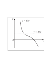
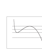
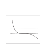
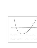
$(a)$	$(b)$	$(c)$	$(d)$

Figure 1: Sketches of the auxiliary function $f(r,q,\Lambda,Q_{m})=-\frac{1}{3}\Lambda r^{3}+r+Q_{m}r^{-1}+{2Q_{m}^{2}}qr^{-3}$. In the points $x=r_{h}$, in which the horizontal mass line $y=2M$ crosses the plot of the function $y=f(r,q,\Lambda,Q_{m})$, the metric function $N(r)$ takes zero values, i.e., the spheres $r_{h}$ are the horizons of the regular nonminimal black holes. The plot of the function $f(r,q,\Lambda,Q_{m})$ depicted in panel $(a)$ has one inflection point and has no extrema; it illustrates the model with one simple horizon only. The plot in panel $(b)$ demonstrates one inflection point and a pair of extrema (the minimum is first, the maximum is second); depending on the mass $M$ one can obtain one or three simple horizons, or one simple and one double horizons (the double horizon appears when the mass-line $y=2M$ touches the plot in an extremum). The plot in panel $(c)$ illustrates the case, when the minimum, the inflection point and the maximum of the plot coincide; there is only one horizon in this case, and it is triple one. Panel $(d)$ illustrates the cases when $f(r,q,\Lambda,Q_{m})$ has no inflection points and has only one extremum, the minimum; in this case there are zero, one double horizon or two simple horizons.

We consider the cosmological constant $\Lambda$ to be positive, zero, and negative. It is reasonable to start with the analysis of the case $\Lambda>0$, i.e., asymptotically dS, which is the most interesting and complex. Then we study the case $\Lambda=0$, i.e., asymptotically flat, in order to recall the partially known results. Finally, we further analyze the case with $\Lambda<0$, i.e., asymptotically AdS.

V Regular nonminimal black holes with positive cosmological constant, $\Lambda>0$

V.1 Introduction

Let us consider spacetimes with dS asymptotics. The model with $\Lambda>0$ has a variety of structures since a cosmological horizon appears in addition to the usual inner and outer horizons. All spacetimes are asymptotically dS.

V.2 Number of horizons and critical masses

V.2.1 Number of horizons

We start with the analysis of the number of horizons. We focus on Eqs. (37)-(38) using the form

$$2M=f(r,q,|\Lambda|,Q_{m})\,,$$ (39)

$$f(r,q,|\Lambda|,Q_{m})\equiv-\frac{|\Lambda|r^{3}}{3}+r+\frac{Q_{m}^{2}}{r}+\frac{{2Q_{m}^{2}}}{r^{3}}q\,,$$ (40)

where we have written $\Lambda=|\Lambda|$ in order to make explicit that the cosmological constant is positive. Clearly, the auxiliary function $f(r,q,|\Lambda|,Q_{m})$ takes negative infinite values at $r\to\infty$, and positive infinite values at $r\to 0$.

The extrema of $f(r,q,|\Lambda|,Q_{m})$ are given through the equation

$$\frac{d}{dr}f(r,q,|\Lambda|,Q_{m})=0\,,$$ (41)

which in turn from Eq. (40) yields the equation

$$|\Lambda|r^{6}-r^{4}+Q_{m}^{2}r^{2}+6{Q_{m}^{2}}q=0\,.$$ (42)

In terms of the auxiliary variable $X\equiv r^{2}$, Eq. (42) gives the cubic equation $|\Lambda|X^{3}-X^{2}+Q_{m}^{2}X+6{Q_{m}^{2}}q=0$. It has three roots $X_{1}$, $X_{2}$, and $X_{3}$, for which the product $X_{1}X_{2}X_{3}=-\frac{6Q_{m}^{2}}{|\Lambda|}q$ is negative, and the sum $X_{1}+X_{2}+X_{3}=\frac{1}{|\Lambda|}$ is positive. There are three cases: (i) there are three real roots and two of them are positive, (ii) there are two coinciding positive roots and one negative, and (iii) one real root is negative and other two roots are complex conjugated. This means that three different situations are available. The configuration can have two extrema (one maximum and one minimum), or it can have two coinciding extrema, or still it can have no extrema.

The points of inflection of $f(r,q,|\Lambda|,Q_{m})$ are given through the equation

$$\frac{d^{2}}{dr^{2}}f(r,q,|\Lambda|,Q_{m})=0\,,$$ (43)

which in turn from Eq. (40) yields the bicubic equation

$$-|\Lambda|r^{6}+{Q_{m}^{2}}r^{2}+12{Q_{m}^{2}}q=0\,.$$ (44)

In terms of the auxiliary variable $Y\equiv r^{2}$, Eq. (44) gives the cubic equation $-|\Lambda|Y^{3}+{Q_{m}^{2}}Y+12{Q_{m}^{2}}q=0$. It has three roots $Y_{1}$, $Y_{2}$, and $Y_{3}$, for which the product $Y_{1}Y_{2}Y_{3}=\frac{12{Q_{m}^{2}}}{|\Lambda|}q$ is positive, and the sum is equal to zero, $Y_{1}+Y_{2}+Y_{3}=0$. This means that only two cases are available: (i) two real roots are negative and one real root is positive, and (ii) the real part of a complex conjugated pair of roots is negative and the only real root is positive. Since negative and complex roots are not physical, we conclude that there exists only one inflection point of the graph of the function $f(r,q,|\Lambda|,Q_{m})$.

The sketches of the corresponding three plots of the function $f(r,q,|\Lambda|,Q_{m})$ are presented in Fig. 1, panels (a), (b) and (c). The mass line $y\equiv 2M$ crosses the corresponding plots at least in one point, meaning that there is at least one horizon. More precisely, depending on the values of parameters $q$, $M$, $Q_{m}$, and $|\Lambda|$, we deal with three independent simple horizons, or with one simple and one double horizon, or with one triple horizon, or even with one simple horizon.

V.2.2 The critical masses

The analysis of horizons and extrema shows that there are two critical masses, $M_{\rm c1}$ and $M_{\rm c2}$, say, for which the corresponding horizons coincides with one of the extrema. For these masses the horizon is in a fact a double horizon, it is degenerate.

One coincidence takes place when the plot of the function $N(r)$ touches the line $N=0$ in its minimum, and another coincidence happens when $N(r)$ touches the line $N=0$ in its maximum. The critical masses can be calculated as

$$M_{\rm c1}=\frac{1}{2}f(r_{\rm c1},q,|\Lambda|,Q_{m})\,,\quad$$ (45)

$$M_{\rm c2}=\frac{1}{2}f(r_{\rm c2},q,|\Lambda|,Q_{m})\,,$$ (46)

where the radii $r_{\rm c1}$ and $r_{\rm c2}$ are obtained as the corresponding solutions of the pair of equations $N(r)=0$ and $\frac{dN(r)}{dr}=0$.

Thus, two critical parameters $M_{\rm c1}$ and $M_{\rm c2}$ appear in the course of analysis. These critical masses can also coincide. In this case we deal with a triple horizon, when the two extrema, the inflection point and all three zeros of the function $N(r)$ coincide.

V.3 The function $N$ and the eight distinct cases

V.3.1 The function $N$ in terms of auxiliary parameters and effective parameters

The family of solutions under discussion is described by four positive parameters with different intrinsic units: $q$, $M$, $Q_{m}$, and $\Lambda$. In order to clarify the fine details of these solutions we use below auxiliary and effective parameters and auxiliary and effective variables. First, we introduce four auxiliary parameters with units of length

$$r_{\Lambda}\equiv\sqrt{\frac{3}{|\Lambda|}}\,,\quad r_{g}\equiv 2M\,,$$

$$r_{q}\equiv({2Q_{m}^{2}}q)^{\frac{1}{4}}\,,\quad r_{Q}\equiv Q_{m}\,.$$ (47)

Second, we construct three effective positive parameters without units, namely,

$$\alpha\equiv\frac{r_{g}}{r_{\Lambda}}\,,\quad\beta\equiv\left(\frac{r_{Q}}{r_{\Lambda}}\right)^{2}\,,\quad\gamma\equiv\left(\frac{r_{q}}{r_{\Lambda}}\right)^{4}\,.$$ (48)

Third, since $\Lambda\neq 0$, in fact here $\Lambda>0$, we introduce the variable $x$ without units through

$$x\equiv\frac{r}{r_{\Lambda}}\,.$$ (49)

We thus use the cosmological scale for the description of the internal structure of the regular nonminimal black holes.

In terms of these variables the metric $N(r)$, given in Eq. (28), is now $N(x)$ and takes the form

$$N(x)=\frac{\gamma+\beta x^{2}-\alpha x^{3}+x^{4}-x^{6}}{x^{4}+\gamma}\,.$$ (50)

Its first derivative is

$$N^{\prime}(x)=-\frac{x\left[2x^{8}-\alpha x^{5}+2x^{4}(\beta+3\gamma)+3\alpha\gamma x-2\beta\gamma\right]}{(x^{4}+\gamma)^{2}}\,,$$ (51)

where ${}^{\prime}\equiv\frac{d\,}{dx}$. Clearly, only the three parameters without units, $\alpha$, $\beta$, and $\gamma$, are the ones that matter in the search for horizons, $N(x)=0$, and in the search for extrema, $N^{\prime}(x)=0$.

In this analysis the masses $M_{\rm c1}$ and $M_{\rm c2}$ given in Eqs. (45)-(46) are important. They give the cases in which there is a double horizon. This double horizon can be an extreme black hole horizon or an extreme cosmological horizon, each with a corresponding radius $x_{\rm c1}$ and $x_{\rm c2}$. The critical masses can coincide giving a triple horizon. The plots of $N(r)$ are presented in Fig. 2. Below we describe the features of the solutions for the different characteristic masses.

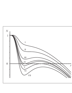
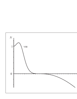
$a$	$b$

Figure 2: $\Lambda>0$. The plots of the metric function $N(r)$ for the nonminimal regular models with $\Lambda>0$. Note that $N(0)=1$ for all curves so that the spacetimes are regular. All the curves have small cavities near the center, repulsive barriers, and a dS asymptotic behavior. In panel $(a)$, seven cases are displayed. Curve I is the case $M=0$. Curve II is representative of the case $0<M\leq M_{\rm N}$ where there is no zone of Newtonian-type attraction. Curve III, for $M_{\rm N}<M<M_{\rm c1}$, describes regular nonminimal stars inside a cosmological horizon, and possessing a Newtonian attraction zone. Curve IV represents the case $M=M_{\rm c1}$, where $M_{\rm c1}$ is a critical mass. There is an extremal nonminimal regular black hole, with the Cauchy and event horizons coinciding, it is a double horizon. Curve V is for $M_{\rm c1}<M<M_{\rm c2}$. Here the nonminimal regular black hole has a Cauchy horizon, an event horizon and a distant cosmological horizon. Curve VI is the case $M=M_{\rm c2}$, where $M_{\rm c1}$ is another critical mass. The event and cosmological horizons coincide, so it is a double horizon. Curve VII for $M_{\rm c2}<M$ represents ultramassive black holes with a regular center and a Cauchy horizon that has turned into a cosmological horizon. In panel $(b)$, curve VIII has a triple horizon of the cosmological type. For this curve four specific points coincide: the inflection point and three zeros of the function $N(r)$.

V.3.2 The eight distinct cases

(i) The case $M=0$

When the mass $M$ vanishes, we deal with a regular nonminimal object that is not a black hole. At $x=0$ there is a minimum with $N(0)=1$; then the function $N(x)$ reaches a maximum at $x=x_{{\rm max}}$, where

$$x_{{\rm max}}=\left[\sqrt{\frac{1}{4}(\beta+3\gamma)^{2}+\beta\gamma}-\frac{1}{2}(\beta+3\gamma)\right]^{\frac{1}{4}}\,.$$ (52)

The zone $0<x<x_{{\rm max}}$ is a central attraction zone. The zone $x_{{\rm max}}<x<\infty$ is a repulsion zone. There is one inflection point of curve $N(x)$ in this zone.

This spacetime has only one horizon, namely, the cosmological horizon at $r_{\rm ch}=\sqrt{\frac{3}{|\Lambda|}}x_{\rm ch}$, where $x_{\rm ch}$ can be found as follows. Define $\gamma_{*}$ and $\Gamma$ as

$$\gamma_{*}=\frac{2}{27}\left[(1+3\beta)^{\frac{3}{2}}-1\right]-\frac{1}{3}\beta\,,$$ (53)

$$\Gamma=1+\frac{27(\gamma-\gamma_{*})}{2(1+3\beta)^{\frac{3}{2}}}\,.$$ (54)

When $\gamma>\gamma_{*}$, one obtains that

$$x_{\rm ch} =\sqrt{\frac{1}{3}+{\bar{\chi}}}\,,$$

$${\bar{\chi}} =\frac{2}{3}\sqrt{1+3\beta}\ \cosh{\left[\frac{1}{3}\log{\left(\Gamma+\sqrt{\Gamma^{2}-1}\right)}\right]}\,.$$ (55)

When $\gamma=\gamma_{*}$, one obtains that

$$x_{\rm ch}=\sqrt{\frac{1}{3}+\chi_{*}}\,,\quad\chi_{*}=\frac{2}{3}\sqrt{1+3\beta}\,.$$ (56)

When $\gamma<\gamma_{*}$, one obtains that

$$x_{\rm ch} =\sqrt{\frac{1}{3}+\tilde{\chi}}\,,$$

$${\tilde{\chi}} =\frac{2}{3}\sqrt{1+3\beta}\ \cos{\left(\frac{1}{3}\arccos{\Gamma}\right)}\,.$$ (57)

This case is illustrated by curve I in Fig. 2.

(ii) The case $0<M\leq M_{\rm N}$

Inside the range $0<M<M_{\rm c1}$ there exists a specific mass value,

$$M_{{\rm N}}=\frac{1}{2}f(r_{{\rm N}},q,|\Lambda|,Q_{m})\,,$$ (58)

which distinguishes the models with no Newtonian-type attraction zone from the ones with a Newtonian-type attraction zone, i.e., with a $1/r$ dominating term in the gravitational potential. For masses in the range $0<M\leq M_{\rm N}$ there is no Newtonian-type attraction zone. The corresponding radius $x_{{\rm N}}$ appears as a solution of the pair of equations, $N^{\prime}(x_{{\rm N}})=0$ and $N^{\prime\prime}(x_{{\rm N}})=0$; i.e., this point of the graph of the function $N(x)$ has a coincidence of extrema points and an inflection point. This limiting case, where the mass is $M_{{\rm N}}$ is illustrated by curve II in Fig. 2 and is representative of the range $0<M\leq M_{N}$. The nonminimal regular objects within this mass range are not black holes, since the single simple horizon is a cosmological horizon.

(iii) The case $M_{\rm N}<M<M_{\rm c1}$

Clearly, within this range the following features can be visualized, see curve III in Fig. 2. There is, first, a central small cavity (between the center $r=0$ and the nearest maximum), second, a repulsion barrier (between the nearest maximum and the following minimum), third, the zone of Newtonian-type attraction, i.e., similar to the $1/r$ behavior of the Newtonian gravitational potential (between the minimum and the final maximum), and fourth, the zone of cosmological repulsion (between the final maximum and infinity). The nonminimal regular objects within this mass range are not black holes, since the single simple horizon is a cosmological horizon.

(iv) The case $M_{\rm c1}=M$

When the mass $M$ has this value, the nonminimal coupled regular black hole is extremal with the inner and the even horizon coinciding. The minimum coincides with a double horizon. There is still an outer cosmological horizon. This is shown in curve IV of Fig. 2.

(v) The case $M_{\rm c1}<M<M_{\rm c2}$

When the mass $M$ is in this range, we deal with regular nonminimal black holes inside a cosmological horizon. Specific features of these solutions are the following, see the curve V in Fig. 2. Each solution of this type displays a small cavity near the regular center, a repulsion barrier, a Cauchy horizon, a black hole region, an event horizon, a zone of Newtonian-type attraction of $1/r$ plus corrections, an intermediate maximum, and a zone of cosmological repulsion.

(vi) The case $M_{\rm c2}=M$

When the mass $M$ has this value, the nonminimal coupled regular black hole is extremal with the even horizon coinciding with the cosmological horizon. The maximum coincides with a double horizon. There is still an inner Cauchy horizon. This is shown in curve VI of Fig. 2. In this case the black hole is a cosmological extremal supermassive regular black hole as the whole visible universe is swallowed by this supermassive object.

(vii) The case $M_{\rm c2}<M$

When the mass exceeds the second critical mass, the Cauchy horizon of the regular nonminimal black hole becomes the cosmological horizon. We deal now with a supermassive black hole with central small cavity, a unified repulsion barrier, and without a standard zone of Newtonian-type attraction, see curve VII on Fig. 2. Since for $M>M_{\rm c2}$ the Cauchy horizon is also a cosmological horizon, the black hole is ultramassive. In such universe there is only one horizon, which is a cosmological one, together with a repulsion zone. In this context this ultramassive black hole is of a new type, for which all three horizons coincide, namely, the Cauchy, event and the cosmological horizons.

(viii) The case $M_{\rm c1}=M_{\rm c2}$

When the critical masses $M_{\rm c1}$ and $M_{\rm c2}$ coincide, two separatrices convert into one curve, depicted in panel (b) of Fig. 2, curve VIII. This curve illustrates the situation, when four specific points of the function $N(x)$ coincide, namely, the maximum, the minimum, the inflection point and the horizon. We deal now with a triple horizon. When $M<M_{\rm c1}=M_{\rm c2}$, the solutions behave like curve III (but without extrema). When $M>M_{\rm c1}=M_{\rm c2}$ the curves look like the curve VII (but without extrema).

VI Regular nonminimal black holes with zero cosmological constant, $\Lambda=0$

VI.1 Introduction

This case has been studied in BaZaPLB and we briefly review the results. All spacetimes are asymptotically flat.

VI.2 Number of horizons and the critical masses

In this case we do not need to introduce variables without units as we did in the previous case. A typical sketch of the auxiliary function $f(r,q,0,Q_{m})$ looks like the curve depicted in panel (d) of Fig. 1. There is a critical mass $M_{\rm c}$, corresponding to the minimum of that curve. Depending on the value of $M$ of the object, the line $y=2M$ can cross the curve $y=f(r,q,0,Q_{m})$ zero times, one time or two times. The corresponding spacetimes have no horizons, when the mass $M$ is less than the critical mass, $M<M_{\rm c}$, it has one horizon, a double one, when $M=M_{\rm c}$, and it has two horizons, when $M>M_{\rm c}$.

In more detail, for $\Lambda=0$, Eqs. (37)-(38) turn into

$$2M=f(r,q,0,Q_{m})\,,$$ (59)

$$f(r,q,0,Q_{m})=r+\frac{{Q_{m}^{2}}}{r}+\frac{{2Q_{m}^{2}}q}{r^{3}}\,.$$ (60)

When the mass line $y=2M$ touches the curve $y=f(r,q,0,Q_{m})$ at the point of minimum, the mass is a critical mass, $M_{{\rm c}}$, given by

$$M_{{\rm c}}=\frac{1}{2}f(r_{\rm c},q,0,Q_{m})\,,$$ (61)

where $r_{\rm c}$ is the critical radius. This radius can be found by imposing $N(r_{{\rm c}})=0$ and $N^{\prime}(r_{{\rm c}})=0$, yielding

$$r_{\rm c}=\sqrt{\frac{{Q_{m}^{2}}}{2}+\sqrt{\frac{{Q_{m}^{4}}}{8}+6{Q_{m}^{2}}q}}\,.$$ (62)

Equations (61)-(62) then give

$$M_{\rm c}=\sqrt{{2Q_{m}^{2}}}\,\frac{\left(1+\frac{8q}{{Q_{m}^{2}}}+\sqrt{1+\frac{24q}{{Q_{m}^{2}}}}\right)}{\left(1+\sqrt{1+\frac{24q}{{Q_{m}^{2}}}}\right)^{\frac{3}{2}}}\,.$$ (63)

The parameter $r_{\rm c}$ is convenient for the analyses. Using it we obtain, in particular, $6{Q_{m}^{2}}q=r_{\rm c}^{2}\left(r_{\rm c}^{2}-{Q_{m}^{2}}\right)$ and $M_{\rm c}=\frac{1}{3r_{\rm c}}(2r_{\rm c}^{2}+{Q_{m}^{2}})$.

VI.3 The function $N$ and the four distinct cases

Now we give the main features of the four distinct types that appear for $\Lambda=0$, see Fig. 3.

(i) The case $M=0$

When $M=0$ we deal with a pure nonminimal object. The metric function $N(r)$ given in Eq. (28) is

$$N(r)=1+\frac{{Q_{m}^{2}}r^{2}}{r^{4}+{2Q_{m}^{2}}q}\,.$$ (64)

and its derivative has also a simple form, $N^{\prime}=\frac{{2Q_{m}^{2}}r}{(r^{4}+{2Q_{m}^{2}}q)^{2}}({2Q_{m}^{2}}q-r^{4})$. The plot of the function $N(r)$, see curve I in Fig. 3, is located above the horizontal line $N=1$ and has a maximum at $r=({2Q_{m}^{2}}q)^{\frac{1}{4}}$, and a minimum at the center. Thus, a Newtonian-type attraction zone is absent now, and there is a repulsion barrier that prolongs itself into infinity. There is no equilibrium point and there are no horizons in the spacetime.

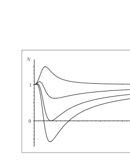
Figure 3: $\Lambda=0$. The plots of the metric function $N(r)$ for the nonminimal regular models with $\Lambda=0$. Note that $N(0)=1$ for all curves so that the spacetimes are regular. All the curves contain a small cavity near the center, a repulsion barrier, and a flat asymptotic behavior. Curve I displays the behavior of $N(r)$, when $M=0$. Curve II is for the case $0<M<M_{\rm c}$. There are no horizons in the spacetime, the object is a regular star. Curve III, for case $M=M_{\rm c}$, is the critical case. There is a double horizon at the minimum of the metric function $N(r)$, i.e., the Cauchy and event horizons coincide. Curve IV describes a black hole with mass exceeding the critical mass $M>M_{\rm c}$, it contains a Cauchy horizon and an event horizon. Curves II, III, and IV, which correspond to massive objects, have zones of Newtonian-type attraction.

(ii) The case $0<M<M_{\rm c}$

When $M<M_{\rm c}$ there are no horizons in the spacetime, and we deal with regular stars. When the mass $M$ is in this range one can find the point of minimum of $N(r)$, $r_{\rm min}$, say, which is an equilibrium point, in which the zones of attraction and repulsion make contact, see curve II in Fig. 3. Since at this point $N^{\prime}(r_{\rm min})=0$, the gravitational force does not act on any massive particle, i.e., a particle can be at rest at this point. Any small perturbation puts this particle to oscillate near this equilibrium point.

(iii) The case $M=M_{\rm c}$

In the critical case $M=M_{\rm c}$ the horizon is double and has radius $r=r_{\rm c}$ given in Eq. (62). The metric function $N(r)$ given in Eq. (28) has for this case the simple form

$$N(r)=\frac{(r-r_{\rm c})^{2}}{r^{4}+{2Q_{m}^{2}}q}\left[r^{2}+\frac{{2Q_{m}^{2}}q}{r_{\rm c}^{2}}\left(\frac{2r}{r_{\rm c}}+1\right)\right]\,.$$ (65)

The multiplier $(r-r_{\rm c})^{2}$ shows explicitly that the horizon at $r=r_{\rm c}$ is a double horizon. In other words, we deal with an extremal regular nonminimal black hole. As $r\to\infty$ the spacetime is asymptotically flat. The plot of the function (65) is presented in Fig. 3 curve III. The curve contains a zone of Newtonian-type attraction, which starts at infinity and finishes at the horizon. The interior of this extremal black hole is regular. It contains a zone near the center which is a nonminimal small cavity, and it also contains a nonminimal repulsion barrier which is locate between the sphere on which $N(r)$ has a maximum and the double horizon.

(iv) The case $M_{\rm c}<M$

When $M_{\rm c}<M$, the interior of the regular black hole contains a nonminimal small cavity and a repulsion barrier that are separated from the exterior by a nonminimal well, see curve IV in Fig. 3. The edge of the well nearest to the center is the Cauchy horizon, the distant edge is the event horizon, it separates the interior from the zone of Newtonian-type attraction with a $\frac{1}{r}$ potential term.

VII Regular nonminimal black holes with negative cosmological constant, $\Lambda<0$

VII.1 Introduction

The case $\Lambda<0$ has some features similar to the $\Lambda=0$ case, with in addition some more structure. All spacetimes are asymptotically AdS.

VII.2 Number of horizons and the critical masses

Let us consider spacetimes with AdS asymptotics, $\Lambda<0$. The case $\Lambda<0$, like the $\Lambda=0$ case, is simpler than the case $\Lambda>0$ and there is no need to introduce variables and parameters with no units.

A typical sketch of the auxiliary function $f(r,q,-|\Lambda|,Q_{m})$ looks like the curve depicted in panel (d) of Fig. 1. In this case there is also a critical mass $M_{\rm c}$ related to the minimum. Depending on the value of $M$ of the object, the line $y=2M$ can cross the curve $y=f(r,q,-|\Lambda|,Q_{m})$ zero times, one time or two times. The corresponding spacetimes have no horizons, when the mass $M$ is less than the critical mass, $M<M_{\rm c}$, it has one horizon, a double one, when $M=M_{\rm c}$, and it has two horizons, when $M>M_{\rm c}$. Since the spacetime is asymptotically AdS for sufficient large radii there is a cosmological attraction.

In more detail, for $\Lambda<0$, Eqs. (37)-(38) turn into

$$2M=f(r,q,-|\Lambda|,Q_{m})\,,$$ (66)

$$f(r,q,-|\Lambda|,Q_{m})\equiv\frac{|\Lambda|r^{3}}{3}+\,r\,+\frac{{Q_{m}^{2}}}{r}+\frac{{2Q_{m}^{2}}}{r^{3}}q\,,$$ (67)

where we have set $\Lambda=-|\Lambda|$. Since the second derivative of the function $f(r,q,-|\Lambda|,Q_{m})$ is positive everywhere, and $f(0,q,-|\Lambda|,Q_{m})=f(\infty,q,-|\Lambda|,Q_{m})=+\infty$, a typical sketch of this function is like panel (d) in Fig. 1. This function has features similar to the function $f(r,q,0,Q_{m})$ analyzed previously.

We can find the critical value of the mass $M_{\rm c}$. It is

$$M_{\rm c}\equiv\frac{1}{2}\left[\frac{|\Lambda|r_{\rm c}^{3}}{3}+r_{\rm c}+\frac{{Q_{m}^{2}}}{r_{\rm c}}+\frac{{2Q_{m}^{2}}}{r_{\rm c}^{3}}q\right]\,,$$ (68)

where $r_{\rm c}$ is the real positive solution of the following bicubic equation

$$|\Lambda|r_{\rm c}^{6}+r_{\rm c}^{4}-{Q_{m}^{2}}r_{\rm c}^{2}-6{Q_{m}^{2}}q=0\,.$$ (69)

In this case there is only one real positive solution. Indeed, if we introduce the quantity $X$ as $X\equiv r^{2}$, we see that the product of the roots of Eq. (69), $X_{1}X_{2}X_{3}=\frac{6{Q_{m}^{2}}q}{|\Lambda|}$ is positive, and the sum $X_{1}+X_{2}+X_{3}=-\frac{1}{|\Lambda|}$ is negative. This can happen in three instances: first, when there are two complex roots and one real positive root, say, $X_{1}>0$; second, when there are three real roots, two of them being negative, and one positive, $X_{1}>0$; third, when $X_{2}=X_{3}<0$, and $X_{1}>0$. In any case, there is only one real positive solution $r_{\rm c}=\sqrt{X_{1}}$ of Eq. (69). Technically, in each of the three mentioned above situations, the unique real positive root $X_{1}$ can be extracted from the three corresponding solutions of the standard Cardano formula, namely,

$$X=Y-\frac{1}{3|\Lambda|}\,,\quad Y_{1}=\mu+\nu\,,$$

$$Y_{2,3}=-\frac{1}{2}(\mu+\nu)\pm i\frac{\sqrt{3}}{2}(\mu-\nu)\,,$$ (70)

where

$$\mu\equiv\left[-\frac{{\cal Q}}{2}+\sqrt{\frac{{\cal P}^{3}}{27}+\frac{{\cal Q}^{2}}{4}}\right]^{\frac{1}{3}}\,,$$

$$\nu\equiv\left[-\frac{{\cal Q}}{2}-\sqrt{\frac{{\cal P}^{3}}{27}+\frac{{\cal Q}^{2}}{4}}\right]^{\frac{1}{3}}\,,$$ (71)

$${\cal Q}\equiv\frac{2+9{Q_{m}^{2}}|\Lambda|-162{Q_{m}^{2}}q|\Lambda|^{2}}{27|\Lambda|^{3}}\,,\quad{\cal P}\equiv-\frac{1+3{Q_{m}^{2}}|\Lambda|}{3|\Lambda|^{2}}\,.$$ (72)

The number of real roots is known to be controlled by the discriminant $\Delta=\frac{{\cal P}^{3}}{27}+\frac{{\cal Q}^{2}}{4}$. There are three real roots, when $\Delta\leq 0$, two roots coincide when the discriminant vanishes $\Delta=0$, and there is one real root when $\Delta>0$.

Let us consider one interesting example exactly solvable. We put ${\cal Q}=0$, i.e.,

$$|\Lambda|=\frac{1}{36q}\left(1+\sqrt{1+\frac{16q}{{Q_{m}^{2}}}}\right)\,.$$ (73)

Then $\Delta=\frac{{\cal P}^{3}}{27}<0$, and we obtain from (70)–(72) three real roots

$$X_{1}=-\frac{1}{3|\Lambda|}+\sqrt{\frac{1+3{Q_{m}^{2}}|\Lambda|}{3|\Lambda|^{2}}}\,,\quad X_{2}=-\frac{1}{3|\Lambda|}\,,$$

$$X_{3}=-\frac{1}{3|\Lambda|}-\sqrt{\frac{1+3{Q_{m}^{2}}|\Lambda|}{3|\Lambda|^{2}}}\,.$$ (74)

The root $X_{1}$ is positive and thus the minimum of the function $f(r,q,-|\Lambda|,Q_{m})$ gives $r_{\rm c}=\sqrt{X_{1}}$, i.e.,

$$r_{\rm c}=\frac{1}{\sqrt{3|\Lambda|}}\sqrt{\sqrt{3+{9}{Q_{m}^{2}}|\Lambda|}-1}\,,$$ (75)

which is the radius corresponding to $M_{\rm c}$ in Eq. (68) in this particular case studied.

VII.3 The function $N(r)$ and the five distinct cases

(i) The case $M=0$

When $M=0$, the metric function is

$$N(r)=1+\frac{r^{2}}{3}\,\frac{3{Q_{m}^{2}}+|\Lambda|r^{4}}{r^{4}+{2Q_{m}^{2}}q}\,.$$ (76)

Clearly, for $M=0$ and negative cosmological constant $N(r)\geq 1$ everywhere, and thus there are no horizons. The derivative

$$N^{\prime}(r)=\frac{2r}{(r^{4}{+}{2Q_{m}^{2}}q)^{2}}\left[\frac{1}{3}|\Lambda|r^{8}{+}{Q_{m}^{2}}r^{4}(2q|\Lambda|{-}1){+}{Q_{m}^{4}}q\right]$$ (77)

is equal to zero at the center $r=0$, and so this point is a local minimum for the metric function $N(r)$. Now, there are still further features depending on whether $6q|\Lambda|<1$, $6q|\Lambda|=1$, or $6q|\Lambda|>1$.

When $6q|\Lambda|<1$, there are two additional extrema, the maximum at

$$r_{\rm max}{=}\left\{\frac{3{Q_{m}^{2}}}{2|\Lambda|}\left[(1{-}2q|\Lambda|){-}\sqrt{(1{-}2q|\Lambda|)^{2}{-}\frac{8}{3}q|\Lambda|}\right]\right\}^{\frac{1}{4}}\,,$$ (78)

and the minimum at

$$r_{\rm min}{=}\left\{\frac{3{Q_{m}^{2}}}{2|\Lambda|}\left[(1{-}2q|\Lambda|){+}\sqrt{(1{-}2q|\Lambda|)^{2}{-}\frac{8}{3}q|\Lambda|}\right]\right\}^{\frac{1}{4}}\,.$$ (79)

In the limiting case $|\Lambda|\to 0$ the minimum drifts to infinity, and the maximum coincides with the value $(2Q_{m}^{2}q)^{\frac{1}{4}}$, thus recovering the case with $\Lambda=0$.

When $6q|\Lambda|=1$, the two radii above coincide with an inflection point, i.e.,

$$r_{\rm inflection}=r_{\rm max}=r_{\rm min}=(6{Q_{m}^{2}}q)^{\frac{1}{4}}\,,$$ (80)

yielding $N(r_{\rm inflection})=1+\sqrt{\frac{{Q_{m}^{2}}}{6q}}$.

When $6q|\Lambda|>1$ there are no additional extrema. This latter case, $6q|\Lambda|>1$, is illustrated by curve I in Fig. 4.

(ii) The case $0<M\leq M_{\rm t}$

For $0<M\leq M_{\rm c}$ there appears another specific mass $M_{\rm t}$, with ${\rm t}$ denoting triple, for which $N^{\prime}(r_{\rm t})=0$ and $N^{\prime\prime}(r_{\rm t})=0$. At this radius, the curve of the metric function $N(r)$ has two extrema coinciding with the inflection point. For $M=M_{\rm t}$ the objects correspond to regular stars since there are no horizons, see curve II in Fig. 4. We note that this curve is of the same type as the curve for the case $M=0$ and $6q|\Lambda|=1$. In the range $0<M\leq M_{\rm t}$ there are no horizons in the spacetime also, and so we also deal with regular stars, of which curve II is representative.

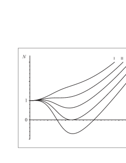
Figure 4: $\Lambda<0$. The plots of the metric function $N(r)$ for the nonminimal regular models with $\Lambda<0$. Note that $N(0)=1$ for all curves so that the spacetimes are regular. All the curves contain a small cavity near the center, a repulsion barrier, and an AdS asymptotic behavior. Curve I displays the behavior of $N(r)$ when $M=0$. Curve II, for $M=M_{\rm t}$ is also representative of the case $0<M<M_{\rm t}$. There are no horizons, the objects are nonminimal stars. Curve III, for $M_{\rm t}<M<M_{\rm c}$ also represents nonminimal stars, in addition it has a flat well with a repulsive barrier followed by a Newtonian-type attraction zone. Curve IV is the critical case $M=M_{\rm c}$ with a double horizon, it describes an extremal black hole. Curve V describes a black hole with $M_{\rm c}<M$, it has a Cauchy horizon and an event horizon.

The plots of the metric function $N(r)$ for the nonminimal regular models with $\Lambda=0$. Note that $N(0)=1$ for all curves so that the spacetimes are regular. All the curves contain a small cavity near the center, a repulsion barrier, and a flat asymptotic behavior. Curve I displays the behavior of $N(r)$, when $M=0$. Curve II is for the case $0<M<M_{\rm c}$. There are no horizons in the spacetime, the object is a regular star. Curve III, for case $M=M_{\rm c}$, is the critical case. There is a double horizon at the minimum of the metric function $N(r)$, i.e., the Cauchy and event horizons coincide. Curve IV describes a black hole with mass exceeding the critical mass $M>M_{\rm c}$, it contains a Cauchy horizon and an event horizon. Curves II, III, and IV, which correspond to massive objects, have zones of Newtonian-type attraction. (iii) The case $M_{\rm t}<M<M_{\rm c}$

When $M_{\rm t}<M<M_{\rm c}$ there are no horizons in the spacetime. The plot of $N(r)$ in this case has a minimum at $r_{\rm min}$, for which $N^{\prime}(r_{\rm min})=0$, see curve III in Fig. 4. Since at $r_{\rm min}$ one has $N^{\prime}(r_{\rm min})=0$, massive particles suffer no force and can be at rest there. However, any small perturbation puts the particle to oscillate near this equilibrium position.

(iv) The case $M=M_{\rm c}$

When $M=M_{\rm c}$, we deal with an extremal regular black hole in an asymptotically AdS spacetime. The horizon is a double horizon, see curve IV in Fig. 4. There are no specific points up to the second order that distinguish the zone of Newtonian-type attraction and the zone of cosmological attraction.

(v) The case $M_{\rm c}<M$

When $M_{\rm c}<M$ we deal with regular black holes with a Cauchy horizon and an event horizon in an asymptotically AdS spacetime, see curve V in Fig. 4.

VIII Conclusions

The solution for the metric potential $N(r)$ that we have found, namely $N=1+\left(\frac{r^{4}}{r^{4}+{2Q_{m}^{2}}q}\right)\left(-\frac{2M}{r}+\frac{{Q_{m}^{2}}}{r^{2}}-\frac{\Lambda}{3}r^{2}\right)$, presents a new exact spherically symmetric static solution of a nonminimal $SU(2)$ Einstein–Yang-Mills theory with a cosmological $\Lambda$ and a Wu-Yang ansatz. The expression for $N(r)$ shows explicitly a four-parameter family of exact solutions. These parameters are the nonminimal parameter $q$, the cosmological constant $\Lambda$, the magnetic charge $Q_{m}$, and the mass $M$.

The most important feature of the family of exact solutions is that it has solutions with horizons depending on the relative values of the parameters. We would like to stress the following details in this context.

For $\Lambda>0$, depending on the values of the parameters, the black hole solution can have three horizons, the Cauchy horizon, the event horizon and the cosmological horizon. When $M<M_{\rm c1}$, the first critical mass value, there is only one horizon, the cosmological horizon. This means that a typical profile of the metric function $N(r)$ contains a central small cavity, a repulsion barrier, a zone of rest for matter near the point of minimum, a Newtonian-type attraction zone, a zone of cosmological acceleration and a zone beyond the cosmological horizon. When $M=M_{\rm c1}$, there is a double extremal horizon, formed by the Cauchy and event horizons together, in addition to the cosmological one. When $M_{\rm c1}<M<M_{\rm c2}$ there are then three separate horizons, the Cauchy, event and cosmological horizons. When $M=M_{\rm c2}$, there is a separate Cauchy horizon, and there is another horizon coincidence, the event horizon and the cosmological horizon come together. In this case the black hole is a cosmological extremal supermassive regular black hole as the whole visible universe is swallowed by this supermassive object. For $M>M_{\rm c2}$ the Cauchy horizon is also a cosmological horizon, the black hole is ultra massive. In such a universe there is only one horizon, which is a cosmological one, together with a repulsion zone. In this context this ultramassive black hole is a new type, in which all three horizons coincide - the Cauchy, event, and cosmological horizons. There is also the case for which $M_{\rm c1}=M_{\rm c2}$ where the three horizons coincide.

For $\Lambda=0$, there is no cosmological horizon and depending on the values of the parameters, the black hole solution can have two horizons - the Cauchy horizon and the event horizon. When the mass is below a critical mass $M_{\rm c}$, there are no horizons. For $M=M_{\rm c}$ a double horizon appears, and when $M$ exceeds $M_{\rm c}$ there are the Cauchy horizon and event horizons.

For $\Lambda<0$, there is also no cosmological horizon and depending on the values of the parameters, the solution can have two horizons - the Cauchy horizon and the event horizon. There is also a critical mass $M_{\rm c}$, below which there are stars and above which there are regular black holes with two horizons. The critical case is a black hole with a double extremal horizon.

Geodesics of massive and massless test particles in these regular black hole geometries display a great variety of cases. Test particles can be in a state of rest on the bottom of the well, or oscillate around this minimum, other particles can overcome the repulsion barrier and be lodged in the central small cavity, and several other trajectories are possible. However, particles cannot leave the well into the exterior since there is a black hole horizon, i.e., there is a one-way membrane.

- (1) W. Scherrer, “Zur Theorie der Elementarteilchen”, Verhandlungen der Schweizerischen Naturforschenden Gesellschaft 121, 86 (1941).
- (2) P. Jordan, “Zur projektiven Relativitätstheorie”, Nachr. Akad. Wiss. Göttingen II, Math.-Phys. Kl. 1945, 39 (1945).
- (3) Y. Thiry, “Les equations de la théorie unitaire de Kaluza”, Comptes Rendus Acad. Sci. 226, 216 (1948).
- (4) C. H. Brans and R. H. Dicke, “Mach’s principle and a relativistic theory of gravitation”, Phys. Rev. 124, 925 (1961).
- (5) H. F. M. Goenner, “On the history of unified field theories. Part II. (ca. 1930 – ca. 1965)”, Living Rev. Relativity 17, 5 (2014). See also, H. F. M. Goenner, “Some remarks on the genesis of scalar-tensor theories”, Gen. Relativ. Gravit. 44, 2077 (2012); arXiv:1204.3455 [gr-qc].
- (6) C. Callan, S. Coleman, and R. Jackiw, “A new improved energy-momentum tensor” Ann. Phys. (N.Y.) 59, 42 (1970).
- (7) V. Faraoni, E. Gunzig, and P. Nardone, “Conformal transformations in classical gravitational theories and in cosmology”, Fundam. Cosm. Phys. 20, 121 (1999); arXiv:gr-qc/9811047.
- (8) A. R. Prasanna, “A new invariant for electromagnetic fields in curved space-time”, Phys. Lett. A 37, 331 (1971).
- (9) I. T. Drummond and S. J. Hathrell, “QED vacuum polarization in a background gravitational field and its effect on the velocity of photons”, Phys. Rev. D22, 343 (1980).
- (10) F. W. Hehl and Yu. N. Obukhov, “How does the electromagnetic field couple to gravity, in particular to metric, nonmetricity, torsion, and curvature?”, in Gyros, Clocks, Interferometers…: Testing relativistic gravity in space, edited by C. Lämmerzahl, C. W. F. Everitt, and F. W. Hehl, Lect. Notes Phys. 562, 479 (2001); arXiv:gr-qc/0001010.
- (11) A. B. Balakin and J. P. S. Lemos, “Non-minimal coupling for the gravitational and electromagnetic fields: A general system of equations”, Classical Quantum Gravity 22, 1867 (2005); arXiv:gr-qc/0503076.
- (12) G. W. Horndeski, “Conservation of charge and second-order gauge-tensor field theories”, Arch. Rat. Mech. Anal. 75, 229 (1981).
- (13) F. Müller-Hoissen, “Modification of Einstein–Yang-Mills theory from dimensional reduction of the Gauss-Bonnet action”, Classical Quantum Gravity 5, L35 (1988).
- (14) A. B. Balakin, H. Dehnen, and A. E. Zayats, “Nonminimal Einstein–Yang-Mills–Higgs theory: Associated, color and color-acoustic metrics for the Wu–Yang monopole model”, Phys. Rev. D76, 124011 (2007); arXiv:0710.5070 [gr-qc].
- (15) A. B. Balakin, H. Dehnen, and A. E. Zayats, “Non-minimal isotropic cosmological model with Yang-Mills and Higgs fields”, Int. J. Mod. Phys. D 17, 1255 (2008); arXiv:0710.4992 [gr-qc].
- (16) A. B. Balakin and W.-T. Ni, “Non-minimal coupling of photons and axions”, Classical Quantum Gravity 27, 055003 (2010); arXiv:0911.2946 [gr-qc].
- (17) G. W. Horndeski, “Static spherically symmetric solutions to a system of generalized Einstein-Maxwell field equations”, Phys. Rev. D17, 391 (1978).
- (18) F. Müller-Hoissen and R. Sippel, “Spherically symmetric solutions of the non-minimally coupled Einstein-Maxwell equations”, Classical Quantum Gravity 5, 1473 (1988).
- (19) G. W. Horndeski, “Birkhoff’s theorem and magnetic monopole solutions for a system of generalized Einstein-Maxwell field equations”, J. Math. Phys. 19, 668 (1978).
- (20) A. B. Balakin, S. V. Sushkov, and A. E. Zayats, “Nonminimal Wu-Yang wormhole”, Phys. Rev. D75, 084042 (2007); arXiv:0704.1224 [gr-qc].
- (21) A. B. Balakin, J. P. S. Lemos, and A. E. Zayats, “Nonminimal coupling for the gravitational and electromagnetic fields: Traversable electric wormholes”, Phys. Rev. D81, 084015 (2010); arXiv:1003.4584 [gr-qc].
- (22) A. B. Balakin and A. E. Zayats, “Dark energy fingerprints in the nonminimal Wu-Yang wormhole structure”, Phys. Rev. D90, 044049 (2014); arXiv:1408.0862 [gr-qc].
- (23) A. B. Balakin, V. V. Bochkarev, and J. P. S. Lemos, “Nonminimal coupling for the gravitational and electromagnetic fields: Black hole solutions and solitons”, Phys. Rev. D77, 084013 (2008); arXiv:0712.4066 [gr-qc].
- (24) A. B. Balakin and A. E. Zayats, “Nonminimal black holes with regular electric field”, Int. J. Mod. Phys. D 24, 1542009 (2015); arXiv:1506.05236 [gr-qc].
- (25) A. B. Balakin and A. E. Zayats, “Non-minimal Wu-Yang monopole”, Phys. Lett. B 644, 294 (2007); arXiv:gr-qc/0612019.
- (26) T. T. Wu and C. N. Yang, “Some solutions of the classical isotopic gauge field equations”, in Properties of Matter under Unusual Conditions, in Honor of Edward Teller’s 60th Birthday, edited by H. Mark and S. Fernbach (Interscience, New York 1969), p. 349.
- (27) Y. Shnir, Magnetic Monopoles (Springer, Berlin 2005).
- (28) J. M. Bardeen, “Non-singular general-relativistic gravitational collapse”, in Abstracts of the 5th International Conference on Gravitation and the Theory of Relativity, edited by V. A. Fock et al. (Tbilisi University Press, Tbilisi, 1968), p. 174.
- (29) I. G. Dymnikova, “Vacuum nonsingular black hole”, Gen. Relativ. Gravit. 24, 235 (1992).
- (30) A. Borde, “Regular black holes and topology change”, Phys. Rev. D55, 7615 (1997); arXiv:gr-qc/9612057 [gr-qc].
- (31) J. J. van der Bij and E. Radu, “Regular and black-hole solutions of the Einstein–Yang-Mills-Higgs equations; the case of nonminimal coupling”, Nucl. Phys. B585, 637 (2000); arXiv:hep-th/0003073.
- (32) E. Ayón-Beato and A. García, “The Bardeen model as a nonlinear magnetic monopole”, Phys. Lett. B 493, 149 (2000); arXiv:gr-qc/0009077.
- (33) J. Matyjasek, “Extremal limit of the regular charged black holes in nonlinear electrodynamics”, Phys. Rev. D70, 047504 (2004); arXiv:gr-qc/0403109.
- (34) D. Horvat, S. Ilijić, Z. Narančić, “Regular and quasi black hole solutions for spherically symmetric charged dust distributions in the Einstein-Maxwell theory”, Classical Quantum Gravity 22, 3817 (2005); arXiv:gr-qc/0409103.
- (35) W. Berej, J. Matyjasek, D. Tryniecki, and M. Woronowicz, “Regular black holes in quadratic gravity”, Gen. Relativ. Gravit. 38, 885 (2006); arXiv:hep-th/0606185.
- (36) K. A. Bronnikov, H. Dehnen, and V. N. Melnikov, “Regular black holes and black universes”, Gen. Relativ. Gravit. 39, 973 (2007); arXiv:gr-qc/0611022.
- (37) J. P. S. Lemos and V. T. Zanchin, “Regular black holes: Electrically charged solutions, Reissner-Nordström outside a de Sitter core”, Phys. Rev. D83, 124005 (2011); arXiv:1104.4790 [gr-qc].
- (38) S. V. Bolokhov, K. A. Bronnikov, and M. V. Skvortsova, “Magnetic black universes and wormholes with a phantom scalar”, Classical Quantum Gravity 29, 245006 (2012); arXiv:1208.4619 [gr-qc].
- (39) N. Uchikata, S. Yoshida, and T. Futamase, “New solutions of charged regular black holes and their stability”, Phys. Rev. D86, 084025 (2012); arXiv:1209.3567 [gr-qc].
- (40) M. Azreg-Aïnou, “Generating rotating regular black hole solutions without complexification”, Phys. Rev. D90, 064041 (2014); arXiv:1405.2569 [gr-qc].
- (41) L. Balart and E. C. Vagenas, “Regular black holes with a nonlinear electrodynamics source”, Phys. Rev. D90, 124045 (2014); arXiv:1408.0306 [gr-qc].
- (42) J. Aftergood and A. DeBenedictis, “Matter conditions for regular black holes in gravity”, Phys. Rev. D90, 124006 (2014); arXiv:1409.4084 [gr-qc].
- (43) B. Toshmatov, A. Abdujabbarov, Z. Stuchlík, and B. Ahmedov, “Quasinormal modes of test fields around regular black holes”, Phys. Rev. D91, 083008 (2015); arXiv:1503.05737 [gr-qc].
- (44) M.-S. Ma, “Magnetically charged regular black hole in a model of nonlinear electrodynamics”, Ann. Phys. (N.Y.) 362, 529 (2015); arXiv:1509.05580 [gr-qc].