Inferring topologies via driving-based generalized synchronization of two-layer networks

Abstract

The interaction topology among the constituents of a complex network plays a crucial role in the network’s evolutionary mechanisms and functional behaviors. However, some network topologies are usually unknown or uncertain. Meanwhile, coupling delay are ubiquitous in various man-made and natural networks. Hence, it is necessary to gain knowledge of the whole or partial topology of a complex dynamical network by taking into consideration communication delay. In this paper, topology identification of complex dynamical networks is investigated via generalized synchronization of a two-layer network. Particularly, based on the LaSalle-type invariance principle of stochastic differential delay equations, an adaptive control technique is proposed by constructing an auxiliary layer and designing proper control input and updating laws so that the unknown topology can be recovered upon successful generalized synchronization. Numerical simulations are provided to illustrate the effectiveness of the proposed method. The technique provides a certain theoretical basis for topology inference of complex networks. In particular, when the considered network is composed of systems with high-dimension or complicated dynamics, a simpler response layer can be constructed, which is conducive to circuit design. Moreover, it is practical to take into consideration perturbations caused by control input. Finally, the method is applicable to infer topology of a subnetwork embedded within a complex system and locate hidden sources. We hope the results can provide basic insight into further research endeavors on understanding practical and economical topology inference of networks.
Keywords: topology identification, two-layer network, stochastic perturbations, coupling delay, generalized synchronization

• December 2015

1 Introduction

Since the groundbreaking works of Watts and Strogatz [1] on small-world networks in 1998 and of Barabási and Albert [2] on scale-free networks in 1999, complex dynamical networks as a new scientific branch have experienced rapid development and have permeated various fields, such as mathematics, computer sciences, engineering sciences and so on [3, 4]. Initial research attention is mainly focused on complex dynamical networks’ statistical properties and dynamical behaviors with previously known topologies. People rarely concentrate on inferring connection topologies of networks, partly because it involves the challenging inverse problem. It is worth noting that topological structures of complex networks play a crucial role in determining their evolutionary mechanisms and functional behaviors [5, 6]. Therefore, it is of necessity and importance to gain knowledge of unknown or uncertain topological structures of complex dynamical networks and provide some theoretical guidance for topology identification of networks.

In the past few years, a great variety of methods have been developed for inferring network topologies, using technologies such as the synchronization-based method [7, 8, 9, 10, 11], compressive sensing [12], Bayesian estimation [13], recurrence [14, 15], Granger causality test [16, 17], node knockout [18], echo state mechanism [19], and so on. Among these methods, the one based on synchronization in which some adaptive controllers are designed so that an auxiliary response network can synchronize with the uncertain network and the topological parameters can be estimated simultaneously, has been paid wide attention to. It is worth mentioning that the synchronization between the two networks is complete outer synchronization [20, 21, 22], which means that each pair of nodes in the drive and response networks manifest completely identical dynamics upon outer synchronization. However, nodes in different networks usually have diverse dynamics, but the networks can still reach harmonious coexistence. This kind of synchronization is called generalized outer synchronization [23], which can be regarded as a special type of generalized synchronization and represents another degree of coherence [24, 25, 26, 27]. A typical example of the generalized outer synchronization is the predator and prey networks. Though individuals in predator network and prey network behave in quite different ways, they may finally coexist in harmony [23]. Therefore, inferring topological structures of complex networks via generalized synchronization is of practical and theoretical significance.

There are many factors influencing network dynamics, such as stochastic perturbations and coupling delay. It is noted that a considerable number of existing works about topology inference focus on networks free of noise perturbations. However, in real-world complex networks, noise is omnipresent. The determinant dynamical network is not real in practice since it usually omit some unknown factors in modeling. For example, the signals transmitted between subsystems of a complex dynamical network are unavoidably subject to stochastic perturbations from environment, which may cause the loss of information contained in these signals [28]. The stochastic uncertainties can have great impact on behaviors of complex networks, such as in genetic oscillator networks, the gene regulation is subject to intracellular and extracellular noise perturbations and environmental fluctuation, so cellular noise will undoubtedly affect the dynamics of the networks quantitatively and qualitatively [29, 30, 31]. Besides, time delay, which is usually caused by finite signal transmission or memory effects, frequently arises in many physical and biological systems such as communication networks, neural networks and so on [32, 33, 34]. Therefore, to investigate and simulate more realistic networks, it is more practical and necessary to take into consideration stochastic perturbations and coupling delay. Moreover, people are usually interested in part of a complex dynamical network. For example, for multi-layer networks [35], one may just want to know the information of one layer of the whole system. From the viewpoint of applicability, inferring the connection pattern of a subnetwork embedded within a complex network is a meaningful and necessary work.

Motivated by above discussions, this paper intends to give some theoretical basis and supports for topology identification of practical complex networks. Particularly, topology inference of complex dynamical networks with coupling delay is investigated via driving-based generalized synchronization in a two-layer network. The interested network is considered as a drive layer, an auxiliary network is constructed as the response layer. In addition, stochastic perturbations caused by control input from the drive layer to the response layer due to information transmission as well as circuit design are also taken into consideration. Some control inputs and updating laws are designed so that nodes in the response layer can reach generalized outer synchronization with their counterparts in the drive layer, and the unknown topology of the drive layer can be adaptively inferred, both in the sense of mean square.

The rest of the paper is organized as follows. In Section 2, the network model and some preliminary lemmas are introduced. In Section 3, by means of adaptive control, several criteria for inferring topologies of complex dynamical networks with coupling delay are derived based on the LaSalle-type invariance principle of stochastic differential delay equations. In Section 4, numerical examples are examined to show the effectiveness of the identification method in the presence of noise perturbations caused by control input and related factors. Furthermore, the method is applicable to recover partial topology of a network and detect hidden sources. Finally, some conclusions and discussions are given in Section 5.

2 Preliminaries and network models

Some necessary notations are first introduced. $\mathbb{R}^{n}$ and $\mathbb{R}^{n\times m}$ denote the $n$-dimensional Euclidean space and the set of all $n\times m$-dimensional real matrices, respectively. $\varotimes$ represents the Kronecker product, and the superscript $\top$ stands for the transpose of a vector or a matrix. $\|\cdot\|$ represents an arbitrary norm. $\lambda_{\mbox{max}}(A)$ is the maximum eigenvalue of matrix $A$. $(\Omega,\mathcal{F},\{\mathcal{F}_{t}\}_{t\geq 0},\mathcal{P})$ is a complete probability space with a filtration $\{\mathcal{F}_{t}\}_{t\geq 0}$ satisfying right continuity and $\mathcal{F}_{0}$ contains all $\mathcal{P}$-null sets. $E\{\cdot\}$ denotes the mathematical expectation. $\dot{x}(t)$ represents the total derivative of $x$ with respect to $t$.

Consider the following general complex dynamics network model with coupling delay,

$$d\mathbf{x}_{i}(t)=\big{(}\mathbf{f}_{i}(t,\mathbf{x}_{i}(t))+\sum_{j=1}^{N}a_{ij}H\mathbf{x}_{j}(t-\tau)\big{)}dt,\,\,\,i=1,2,\cdots,N,$$ (1)

where $\mathbf{x}_{i}=(x_{i1},x_{i2},\cdots,x_{im})^{T}\in\mathbb{R}^{m}$ is the state vector of the $i$-th node. $\mathbf{f}_{i}:\mathbb{R}_{+}\times\mathbb{R}^{m}\rightarrow\mathbb{R}^{m}$ is a smooth nonlinear vector-valued function which determines the intrinsic dynamical behavior of the $i$-th node in network (1). $H\in\mathbb{R}^{m\times m}$ is the inner coupling matrix linking interacted component variables, and $A=(a_{ij})_{N\times N}\in\mathbb{R}^{N\times N}$ is the unknown or uncertain coupling configuration matrix representing the network’s topological structure, whose entries are defined as follows: if there is a link from node $j$ to node $i$, then $a_{ij}\neq 0$, otherwise, $a_{ij}=0(i\neq j)$, and $a_{ii}=-\sum\limits_{j=1,j\neq i}^{N}a_{ij},(i=1,2,\cdots,N)$. $\tau$ represents the information transmission delay between connected nodes.

It is worth-noting that network topologies play a pivotal role in determining the emergence of collective behaviors and governing the main features of relevant processes that take place in complex networks. Therefore, it is of necessity and importance to gain knowledge of the intrinsic topology, which is usually unknown in many practical situations. In network (1), the node dynamics $\mathbf{f}_{i}$, the coupling matrix $H$, and the communication delay $\tau$ between nodes are supposed to be known. Our purpose is to infer the unknown topological matrix $A$ based on signals output from the considered network, which will probably be contaminated by noise. For this purpose, some necessary concepts and lemmas of stochastic differential equations are presented.

Consider a nonautonomous $n$-dimensional stochastic differential delay equation

$$d\mathbf{x}(t)=\mathbf{f}(t,\mathbf{x}(t),\mathbf{x}(t-\tau))dt+\mathbf{g}(t,\mathbf{x}(t),\mathbf{x}(t-\tau))d\mathbf{w}(t)$$ (2)

on $t\geq 0$ with initial value $\xi\in C_{\mathcal{F}_{0}}^{b}([-\tau,0];\mathbb{R}^{n})$, where $C_{\mathcal{F}_{0}}^{b}([-\tau,0];\mathbb{R}^{n})$ denotes the family of all $\mathcal{F}_{0}$-measurable bounded $C([-\tau,0];\mathbb{R}^{n})$-valued random variables, the measurable functions $\mathbf{f}$ and $\mathbf{g}:\mathbb{R}_{+}\times\mathbb{R}^{n}\times\mathbb{R}^{n}\rightarrow\mathbb{R}^{n}$ satisfy the local Lipschitz condition and the linear growth condition [36]. Then, for any initial value $\xi\in C_{\mathcal{F}_{0}}^{b}([-\tau,0];\mathbb{R}^{n})$, Eq.(2) has a unique solution denoted by $\mathbf{x}(t;\xi)$ on $t\geq-\tau$. Moreover, assume $\mathbf{f}(t,0,0)=\mathbf{g}(t,0,0)=0$, then Eq.(2) admits a trivial solution $\mathbf{x}(t,0)\equiv 0$.

Let $C^{1,2}(\mathbb{R}_{+}\times\mathbb{R}^{n};\mathbb{R}_{+})$ denote the family of all nonnegative functions $V(t,\mathbf{x})$ on $\mathbb{R}_{+}\times\mathbb{R}^{n}$ which are continuously twice differentiable in $\mathbf{x}$ and once differentiable in $t$. Then the diffusion operator $\mathcal{L}$ acting on $V(t,\mathbf{x})$ is

$$\mathcal{L}V=V_{t}(t,\mathbf{x})+V_{x}(t,\mathbf{x})\mathbf{f}(t,\mathbf{x})+\frac{1}{2}\mbox{trace}[\mathbf{g}^{T}(t,\mathbf{x})V_{xx}(t,\mathbf{x})\mathbf{g}(t,\mathbf{x})],$$ (3)

where $V_{t}(t,\mathbf{x})=\frac{\partial V(t,\mathbf{x})}{\partial t}$, $V_{x}(t,\mathbf{x})=\left(\frac{\partial V(t,\mathbf{x})}{\partial\mathbf{x}_{1}},\frac{\partial V(t,\mathbf{x})}{\partial\mathbf{x}_{2}},\cdots,\frac{\partial V(t,\mathbf{x})}{\partial\mathbf{x}_{n}}\right)$, $V_{xx}(t,\mathbf{x})=\left(\frac{\partial^{2}V(t,\mathbf{x})}{\partial\mathbf{x}_{i}\partial\mathbf{x}_{j}}\right)_{n\times n}$.

Lemma 2.1

[36] Assume that there is a function $V\in C^{1,2}(\mathbb{R}_{+}\times\mathbb{R}^{n};\mathbb{R}_{+})$, a function $\gamma\in L^{1}(\mathbb{R}_{+};\mathbb{R}_{+})$ and continuous functions $\omega_{1},\omega_{2}:\mathbb{R}^{n}\rightarrow\mathbb{R}_{+}$ such that

$$\mathcal{L}V(t,\mathbf{x},\mathbf{y})\leq\gamma(t)-\omega_{1}(\mathbf{x})+\omega_{2}(\mathbf{y}),\,\,\,(t,\mathbf{x},\mathbf{y})\in\mathbb{R}_{+}\times\mathbb{R}^{n}\times\mathbb{R}^{n},$$

$$\omega_{1}(\mathbf{x})>\omega_{2}(\mathbf{x}),\,\,\,\forall\mathbf{x}\neq 0,$$

$$\lim_{\parallel\mathbf{x}\parallel\rightarrow\infty}\inf_{0\leq t<\infty}V(t,\mathbf{x})=\infty.$$

Then

$$\lim_{t\rightarrow\infty}\mathbf{x}(t;\xi)=0\,\,\,a.s.$$ (4)

for any initial value $\xi\in C_{\mathcal{F}_{0}}^{b}([-\tau,0];\mathbb{R}^{n})$.

Lemma 2.2

[37] For any vectors $\mathbf{x},\mathbf{y}\in\mathbb{R}^{n}$ and a symmetric positive definite matrix $Q\in\mathbb{R}^{n\times n}$, the following inequality holds: $2\mathbf{x}^{T}\mathbf{y}\leq\mathbf{x}^{T}Q\mathbf{x}+\mathbf{y}^{T}Q^{-1}\mathbf{y}$.

3 Results

To infer the unknown topology of network (1), an auxiliary system consisting of an identical number of nodes as that of network (1) is constructed as follows:

$$d\mathbf{y}_{i}(t)=\big{(}\mathbf{g}_{i}(t,\mathbf{y}_{i}(t))+\mathbf{u}_{i}\big{)}dt+\psi_{i}(t)d\mathbf{w}_{i}(t),~{}~{}i=1,2,\cdots,N,$$ (5)

where $\mathbf{y}_{i}=(x_{i1},x_{i2},\cdots,x_{in})^{T}\in\mathbb{R}^{n}$ is the state vector of the $i$-th node, $\mathbf{g}_{i}:\mathbb{R}_{+}\times\mathbb{R}^{n}\rightarrow\mathbb{R}^{n}$ is a smooth nonlinear vector-valued function governing the dynamical behavior of the $i$-th node. Furthermore, $\mathbf{u}_{i}$ is the control input to be designed for the $i$-th node. The noise term is utilized to describe perturbations caused by the control input, where information collected from the drive layer will be put into the response layer and thus noise will emerge due to information transmission and inaccurate circuit design. Specifically, $\mathbf{w}_{i}(t)$ is an $n$-dimensional Brownian motion defined on the probability space $(\Omega,\mathcal{F},\{\mathcal{F}_{t}\}_{t\geq 0},\mathcal{P})$ with

$$E\{\mathbf{w}_{i}(t)\}=0,{\color[rgb]{0,0,1}E\{\mathbf{w}_{i}^{2}(t)\}=t},E\{\mathbf{w}_{i}(s)\mathbf{w}_{i}(t)\}=\min\{s,t\}(s\neq t),E\{\mathbf{w}_{i}(t)\mathbf{w}_{j}(t)\}=0(i\neq j),$$

$\psi_{i}(t)$ is the vector-form noise intensity function which describes the intensity of uncertain perturbations to the $i$-th node.

Since each node in the auxiliary network (5) receives driving signals from its counterpart in the considered network (1), the two networks form a two-layer network with one-to-one unidirectional connections. In the following, network (1) is regarded as the drive layer, and network (5) is regarded as the response layer. To infer topologies of the considered network, controllers are designed so that the response layer can harmoniously oscillate with the drive layer and topological parameters of network (1) are reconstructed. In addition, due to the fact that node dynamics in the two layers are usually different, one will use generalized outer synchronization rather than complete outer synchronization to characterize the harmonious oscillation between the two layers.

Particularly, let $\mathbf{e}_{i}(t)=\mathbf{y}_{i}(t)-\phi_{i}(\mathbf{x}_{i}(t))$ denote the generalized outer synchronization error between the $i$-th nodes in the two layers, where $\phi_{i}:\mathbb{R}^{m}\rightarrow\mathbb{R}^{n}$ is a once continuously differentiable vector function describing functional relationships between corresponding nodes. The two network layers are said to achieve generalized outer synchronization (or one can say the two-layer network achieves generalized synchronization) in the sense of mean square if

$$\lim_{t\rightarrow\infty}E\|\mathbf{e}_{i}(t)\|^{2}=0,\,\,\,i=1,2,\cdots,N.$$

Let

$$\dot{\hat{a}}_{ij}(t)=-\delta_{ij}\mathbf{e}_{i}^{T}(t)D\phi_{i}(\mathbf{x}_{i})H\mathbf{x}_{j}(t-\tau),\,\,\,i,j=1,2,\cdots,N$$ (6)

be updating laws to track the unknown topological parameters $a_{ij}~{}(i,j=1,2,\cdots,N)$ in the drive layer. The control input $\mathbf{u}_{i}$ for the $i$-node in the response layer and the adaptive feedback gain are thus designed as

$$\mathbf{u}_{i}(t)= D\phi_{i}(\mathbf{x}_{i})\mathbf{f}_{i}(t,\mathbf{x}_{i}(t))-\mathbf{g}_{i}(t,\phi_{i}(\mathbf{x}_{i}(t)))$$ (7)

$$+D\phi_{i}(\mathbf{x}_{i})\sum_{j=1}^{N}\hat{a}_{ij}H\mathbf{x}_{j}(t-\tau)-d_{i}(t)\mathbf{e}_{i}(t),$$

and

$$\dot{d}_{i}(t)=k_{i}\mathbf{e}_{i}^{T}(t)\mathbf{e}_{i}(t),\,\,\,i=1,2,\cdots,N,$$ (8)

respectively, where $D\phi_{i}(\mathbf{x}_{i})$ is the Jacobian matrix of $\phi_{i}(\mathbf{x}_{i}(t))$, $\delta_{ij}>0$ and $k_{i}>0$ are arbitrary constants.

Let $\tilde{a}_{ij}=\hat{a}_{ij}-a_{ij}$, then the error dynamics between the layers (1) and (5) can be described as

$$d\mathbf{e}_{i}(t) = d\mathbf{y}_{i}(t)-D\phi_{i}(\mathbf{x}_{i})d\mathbf{x}_{i}(t)$$ (9)

$$= \big{(}\mathbf{g}_{i}(t,\mathbf{y}_{i}(t))-D\phi_{i}(\mathbf{x}_{i})\mathbf{f}_{i}(t,\mathbf{x}_{i}(t))-D\phi_{i}(\mathbf{x}_{i})\sum_{j=1}^{N}a_{ij}H\mathbf{x}_{j}(t-\tau)$$

$$+\mathbf{u}_{i}\big{)}dt+\psi_{i}(t)d\mathbf{w}_{i}(t)$$

$$= \big{(}\mathbf{g}_{i}(t,\mathbf{y}_{i}(t))-\mathbf{g}_{i}(t,\phi_{i}(\mathbf{x}_{i}(t)))+D\phi_{i}(\mathbf{x}_{i})\sum_{j=1}^{N}\tilde{a}_{ij}H\mathbf{x}_{j}(t-\tau)$$

$$-d_{i}(t)\mathbf{e}_{i}(t)\big{)}dt+\psi_{i}(t)d\mathbf{w}_{i}(t),\,\,\,i=1,2,\cdots,N,$$

Assumption 3.1

(Lipschitz condition)For the nonlinear vector function $\mathbf{g}_{i}(\cdot)$, there exists a positive constant $\alpha_{i}$ such that for $i=1,2,\cdots,N$,

$$\|\mathbf{g}_{i}(t,\mathbf{y}(t))-\mathbf{g}_{i}(t,\mathbf{x}(t))\|\leq\alpha_{i}\|\mathbf{y}(t)-\mathbf{x}(t)\|$$

holds for any $\mathbf{x}(t),\mathbf{y}(t)\in\mathbb{R}^{n}$.

Assumption 3.2

Suppose that $\psi_{i}(t)$ is bounded, and there exist nonnegative constants $\mu_{i},\nu_{i}\geq 0$ such that for $i=1,2,\cdots,N$,

$$\mbox{trace}(\psi_{i}^{T}(t)\psi_{i}(t))\leq 2\mu_{i}\mathbf{e}_{i}^{T}(t)\mathbf{e}_{i}(t)+2\nu_{i}\mathbf{e}_{i}^{T}(t-\tau)\mathbf{e}_{i}(t-\tau).$$

Remark 3.1

For the purpose of inferring the unknown topology of the drive layer, a response layer is constructed. The noise term in the constructed auxiliary network is utilized to describe perturbations caused by the control input, where information collected from the drive layer (such as $\mathbf{x}_{i}$) will be put into the response layer and thus noise will emerge due to information transmission as well as inaccurate circuit design. During this process, the noise is inevitably influenced by both the input signal $\mathbf{x}_{i}$ and response dynamics $\mathbf{y}_{i}$. This is a commonly-employed condition in many literatures [38, 39].

Assumption 3.3

$\{D\phi_{i}(\mathbf{x}_{i})H\mathbf{x}_{i}(t)\}_{i=1}^{N}$ are linearly independent on the orbit $\{\mathbf{x}_{i}(t)\}_{i=1}^{N}$ of the generalized outer synchronization manifold $\{\mathbf{y}_{i}(t)=\phi_{i}(\mathbf{x}_{i}(t))\}_{i=1}^{N}$ between the two network layers.

With these assumptions, the main topology identification result based on generalized synchronization in a two-layer network is given as follows.

Theorem 3.1

Let Assumptions 3.1-3.3 hold. Then the uncertain coupling configuration matrix $A$ of the considered network (1) can be identified by the estimated values $\hat{A}$ with probability one via adaptive controllers and updating laws (6)-(8). Meanwhile, the response layer (5) reaches generalized outer synchronization with the drive layer (1) in mean square.

Proof. Consider the following Lyapunov function $V\in C^{1,2}(\mathbb{R}_{+}\times\mathbb{R}^{nN+N^{2}+N};\mathbb{R}_{+})$,

$$V(t;\mathbf{e}_{i},\tilde{a}_{ij},d_{i})=\frac{1}{2}\sum_{i=1}^{N}\mathbf{e}_{i}^{T}(t)\mathbf{e}_{i}(t)+\frac{1}{2}\sum_{i=1}^{N}\sum_{j=1}^{N}\frac{1}{\delta_{ij}}\tilde{a}_{ij}^{2}+\frac{1}{2}\sum_{i=1}^{N}\frac{1}{k_{i}}(d_{i}(t)-d_{i}^{*})^{2},$$ (10)

where $d_{i}^{*}~{}(i=1,2,\cdots,N)$ are positive constants to be determined.

The diffusion operator $\mathcal{L}$ defined in (3) onto the function $V$ along the trajectories of the error dynamics (9) gives

$$\mathcal{L}V=\sum_{i=1}^{N}\mathbf{e}_{i}^{T}(t)\big{(}\mathbf{g}_{i}(t,\mathbf{y}_{i}(t))-\mathbf{g}_{i}(t,\phi_{i}(\mathbf{x}_{i}(t)))+D\phi_{i}(\mathbf{x}_{i})\sum_{j=1}^{N}\tilde{a}_{ij}H\mathbf{x}_{j}(t-\tau)-d_{i}(t)\mathbf{e}_{i}(t)\big{)}$$

$$\qquad\quad+\sum_{i=1}^{N}\sum_{j=1}^{N}\frac{1}{\delta_{ij}}\tilde{a}_{ij}\dot{\hat{a}}_{ij}+\sum_{i=1}^{N}\frac{1}{k_{i}}(d_{i}(t)-d_{i}^{*})\dot{d}_{i}(t)+\frac{1}{2}\sum_{i=1}^{N}\mbox{trace}(\psi_{i}^{T}(t)\psi_{i}(t)).$$

Together with the updating laws (6) and (8), one gets

$$\mathcal{L}V=\sum_{i=1}^{N}\mathbf{e}_{i}^{T}(t)\big{(}\mathbf{g}_{i}(t,\mathbf{y}_{i}(t))-\mathbf{g}_{i}(t,\phi_{i}(\mathbf{x}_{i}(t)))+D\phi_{i}(\mathbf{x}_{i})\sum_{j=1}^{N}\tilde{a}_{ij}H\mathbf{x}_{j}(t-\tau)-d_{i}(t)\mathbf{e}_{i}(t)\big{)}$$

$$\qquad\quad-\sum_{i=1}^{N}\sum_{j=1}^{N}\tilde{a}_{ij}\mathbf{e}_{i}^{T}(t)D\phi_{i}H\mathbf{x}_{j}(t-\tau)+\sum_{i=1}^{N}(d_{i}(t)-d_{i}^{*})\mathbf{e}_{i}^{T}(t)\mathbf{e}_{i}(t)+\frac{1}{2}\sum_{i=1}^{N}\mbox{trace}(\psi_{i}^{T}(t)\psi_{i}(t))$$

$$\qquad\!=\sum_{i=1}^{N}\mathbf{e}_{i}^{T}(t)\big{(}\mathbf{g}_{i}(t,\mathbf{y}_{i}(t))-\mathbf{g}_{i}(t,\phi_{i}(\mathbf{x}_{i}(t)))\big{)}-\sum_{i=1}^{N}d_{i}^{*}\mathbf{e}_{i}^{T}(t)\mathbf{e}_{i}(t)+\frac{1}{2}\sum_{i=1}^{N}\mbox{trace}(\psi_{i}^{T}(t)\psi_{i}(t)).$$

Following from Assumptions 3.1 and 3.2, one has

$$\mathcal{L}V \leq \sum_{i=1}^{N}(\alpha_{i}-d_{i}^{*})\mathbf{e}_{i}^{T}(t)\mathbf{e}_{i}(t)+\sum_{i=1}^{N}\big{(}\mu_{i}\mathbf{e}_{i}^{T}(t)\mathbf{e}_{i}(t)+\nu_{i}\mathbf{e}_{i}^{T}(t-\tau)\mathbf{e}_{i}(t-\tau)\big{)}$$

$$\leq \sum_{i=1}^{N}(\alpha_{i}+\mu_{i}-d_{i}^{*})\mathbf{e}_{i}^{T}(t)\mathbf{e}_{i}(t)+\sum_{i=1}^{N}\nu_{i}\mathbf{e}_{i}^{T}(t-\tau)\mathbf{e}_{i}(t-\tau).$$

Let $\mathbf{e}(t)=(\mathbf{e}_{1}(t)^{T},\mathbf{e}_{2}(t)^{T},\dots,\mathbf{e}_{N}(t)^{T})^{T}\in\mathbb{R}^{nN}$, $\alpha=\max_{1\leq i\leq N}\{\alpha_{i}\}$, $d^{*}=\max_{1\leq i\leq N}\{d_{i}^{*}\}$, $\mu=\max_{1\leq i\leq N}\{\mu_{i}\}$, $\nu=\max_{1\leq i\leq N}\{\nu_{i}\}$, then

$$\mathcal{L}V \leq -(d^{*}-\alpha-\mu)\mathbf{e}^{T}(t)\mathbf{e}(t)+\nu\mathbf{e}_{i}^{T}(t-\tau)\mathbf{e}_{i}(t-\tau)$$

$$\triangleq -\omega_{1}(\mathbf{e}(t))+\omega_{2}(\mathbf{e}(t-\tau)),$$

where $\omega_{1}(\mathbf{x})\triangleq(d^{*}-\alpha-\mu)\mathbf{x}^{T}\mathbf{x}$, $\omega_{2}(\mathbf{x})\triangleq\nu\mathbf{x}^{T}\mathbf{x}$.

It is obvious that if $d^{*}>\alpha+\mu+\nu$, then $\omega_{1}(\mathbf{x})>\omega_{2}(\mathbf{x})$ for any $\mathbf{x}\neq 0$. In addition, $\lim_{\|\mathbf{e}\|\rightarrow\infty}\inf_{0\leq t<\infty}V=\infty$ and $\psi_{i}$ is bounded. Following from Lemma 2.1, one obtains $\lim_{t\rightarrow\infty}\mathbf{e}(t)=0$ a.s., which implies that $\lim_{t\rightarrow\infty}E\|\mathbf{e}_{i}(t)\|^{2}=0$ and the solutions regarding Eqs. (6), (8) and (9) starting from $\mathbb{R}^{nN+N^{2}+N}$ will asymptotically stabilize at $M=\{(\mathbf{e}_{i},\tilde{a}_{ij},d_{i})\in\mathbb{R}^{nN+N^{2}+N}:\mathbf{e}=0\}$ with probability one. In addition, together with system (9) and Assumption 3.3, one gets $M=\{\mathbf{e}=0,\tilde{a}_{ij}=0,d_{i}=constants\}$ for $i,j=1,2,\dots,N$. That is, with the controllers and updating laws (6)-(8), the response network layer (5) reaches generalized outer synchronization with the drive layer (1) and the unknown coupling configuration matrix $A$ is successfully identified by $\hat{A}$ in the sense of mean square. This completes the proof.

Remark 3.2

It is clear that the coupling configuration matrix $A$ is not required to be symmetric, irreducible or diffusive, and the inner coupling matrix $H$ is not necessarily symmetric. This indicates that the unknown structure of network (1) can be undirected or directed, connected or disconnected. It may even contain isolated nodes or clusters. In addition, there is not any constraint imposed on the nodal or coupling form in the constructed response network layer (5). Moreover, each node in the two-layer network may have various dynamical behaviors. Therefore, the identification technique is applicable to a large variety of complex dynamical networks with communication delay.

Remark 3.3

Unlike many previous schemes [40, 7, 8, 9, 10], the constructed auxiliary network can be consisting of any kind of dynamical nodes other than nodes with identical dynamics as their counterparts in the drive layer. Therefore, if the considered network is composed of nodes carrying very complicated node dynamics or high node dimensions, one can design a response layer using nodes with much simpler dynamics. Moreover, the topological structure of the auxiliary layer can be any form, which does not affects the inferring topology for the drive layer. Hence, the form of auxiliary system is more practical for circuit design.

Remark 3.4

It should be especially pointed out that the linear independence condition in Assumption 3.3 is a very essential condition for guaranteeing successful topology identification. The linear independence condition is needed for theoretical analysis. However, it is very difficult to verify this condition in practice. Chen et al. declared that complete synchronization in the unknown network will make the linearly independence condition unsatisfied, then the identification of the unknown topology is impossible [41]. They also found that partial synchronization in the unknown network implies a part of topology being unidentifiable, and the results can be extended to projection synchronization and some generalized synchronization. In addition, Liu et al. declared that synchronization of the drive network is harmful to the identification of the topological structure as it is difficult to satisfy Assumption 3.3 [9]. They also pointed out that it is often difficult to recover the topology of an unknown network with identical nodes, since the network easily reaches some kind of inner synchronization. Therefore, it is practical to check whether the nodes of the unknown network achieve synchronization instead of checking the linear independence condition. Moreover, diverse dynamics and chaotic behaviors of the nodes within the unknown network can facilitate topology identification.

Based on Theorem 3.1, one can easily derive the following corollaries.

Corollary 3.1

Suppose Assumptions 3.1-3.3 hold. If the considered network (1) is free of coupling delay, that is, $\tau=0$, then the uncertain coupling configuration matrix $A$ can be inferred by $\hat{A}$ in mean square via the controllers

$$\mathbf{u}_{i}(t)=D\phi_{i}(\mathbf{x}_{i})\mathbf{f}_{i}(t,\mathbf{x}_{i}(t))-\mathbf{g}_{i}(t,\phi_{i}(\mathbf{x}_{i}(t)))+D\phi_{i}(\mathbf{x}_{i})\sum_{j=1}^{N}\hat{a}_{ij}H\mathbf{x}_{j}(t)-d_{i}(t)\mathbf{e}_{i}(t),$$ (11)

and updating laws

$$\dot{d}_{i}(t)=k_{i}\mathbf{e}_{i}^{T}(t)\mathbf{e}_{i}(t),\,\,\,\dot{\hat{a}}_{ij}(t)=-\delta_{ij}\mathbf{e}_{i}^{T}(t)D\phi_{i}(\mathbf{x}_{i})H\mathbf{x}_{j}(t),\,\,\,i,j=1,2,\cdots,N,$$ (12)

where $k_{i},\delta_{ij}~{}(i,j=1,2,\cdots,N)$ are arbitrary positive constants.

Corollary 3.2

Suppose Assumptions 3.1 and 3.3 hold. If there is no noise perturbations, that is, $\psi_{i}(t)=0,(i=1,2,\cdots,N)$, then the uncertain coupling configuration matrix $A$ can be identified by the estimated values $\hat{A}$ via updating laws and controllers (6)-(8) upon successful generalized out synchronization in the two network layers (1) and (5).

Corollary 3.3

Suppose Assumptions 3.1-3.3 hold. If the $i$-th node in the response layer (5) is designed to be the same as its counterpart in the drive layer (1), that is, $\mathbf{f}_{i}(\cdot)=\mathbf{g}_{i}(\cdot)$, then the uncertain coupling configuration matrix $A$ can be identified by the estimated values $\hat{A}$ and complete outer synchronization between the two network layers can be realized in mean square via the controllers

$$\mathbf{u}_{i}(t)=\sum_{j=1}^{N}\hat{a}_{ij}H\mathbf{y}_{j}(t-\tau)-d_{i}(t)\mathbf{e}_{i}(t),\,\,\,i=1,2,\cdots,N,$$ (13)

and updating laws

$$\dot{d}_{i}(t)=\,\,k_{i}\mathbf{e}_{i}^{T}(t)\mathbf{e}_{i}(t),\,\,\,\dot{\hat{a}}_{ij}(t)=-\delta_{ij}\mathbf{e}_{i}^{T}(t)D\phi_{i}(\mathbf{x}_{i})H\mathbf{y}_{j}(t-\tau),\,\,\,i,j=1,2,\cdots,N,$$ (14)

where $k_{i},\delta_{ij}~{}(i,j=1,2,\cdots,N)$ are arbitrary positive constants.

Furthermore, if the response layer (5) receives input signals from the drive layer (1) free of noise perturbations and there is no information transmission delay between node pairs, then with controllers (11) and (12), the uncertain coupling configuration matrix $A$ can be identified by the estimated values $\hat{A}$ upon generalized outer synchronization between the two layers. This result covers the latest result presented in [42]. Moreover, the auxiliary layer (5) and controllers (11) are much simpler than their counterparts in [42]. It is worth mentioning that the auxiliary network layer (5) constructed in this paper contains no connections between its nodes, thus the auxiliary system and controllers are much simpler and more practical than previous results [7, 8, 9, 10], [42].

4 Numerical simulations

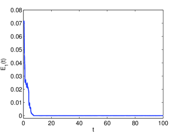
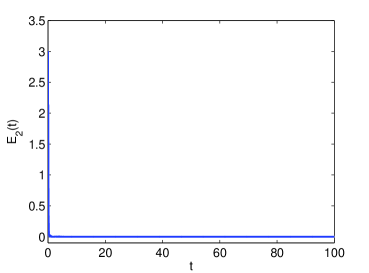
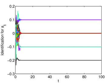
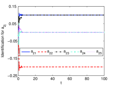
Figure 1: Identification error (left) and synchronization error (right) of the two-layer Lü-Chua network.

Figure 2: Time evolution of $\hat{a}_{ij}~{}(i,j=1,2,...,5)$ (left) and $\hat{a}_{2j}~{}(j=1,2,...,5)$ (right) of the two-layer Lü-Chua network.

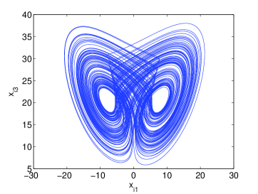
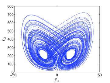
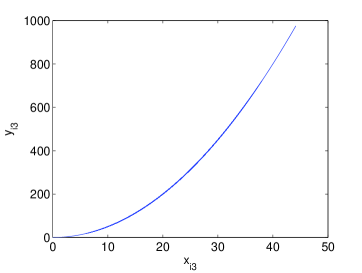
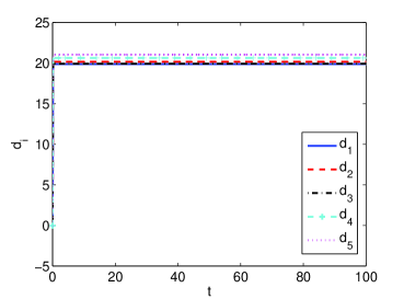
Figure 3: Phase diagrams of node dynamics in the two-layer Lü-Chua network. Left: projection in the $(x_{i1},x_{i3})$-plane of node 2 in the drive layer; right: projection in the $(y_{i1},y_{i3})$-plane of the node 2 in the response layer.

Figure 4: Relationship between the component variables $x_{i3}$ and $y_{i3}$ of node 2 (left) and time evolution of adaptive feedback gains $d_{i}~{}(i=1,2,...,5)$ (right) of the two-layer Lü-Chua network.

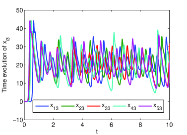
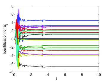
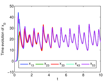
Figure 5: Time evolution of the component variables $x_{i3}~{}(i=1,2,...,5)$ in the drive layer of the two-layer Lü-Chua network with successful topology identification.

Figure 6: Identification failure due to unsatisfied linear independence condition. $\hat{a}_{ij}~{}(i,j=1,2,...,5)$ (left) and time evolution of the component variables $x_{i3}~{}(i=1,2,...,5)$ in the drive layer (right) of the two-layer Lü-Chua network.

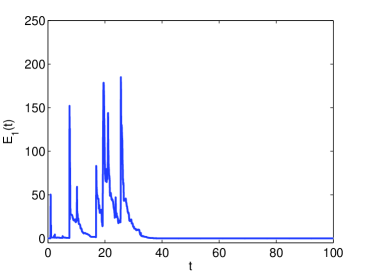
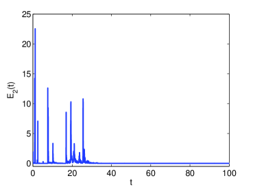
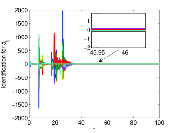
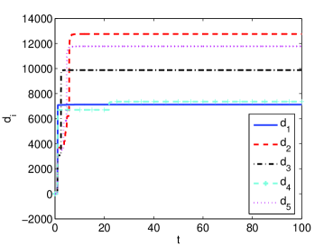
Figure 7: Identification error (left) and synchronization error (right) of the two-layer hyperchaotic Lü-Duffing network.

Figure 8: Time evolution of $\hat{a}_{ij}~{}(i,j=1,2,...,5)$ (left) and adaptive feedback gains $d_{i}~{}(i=1,2,...,5)$ (right) of the two-layer hyperchaotic Lü-Duffing network.

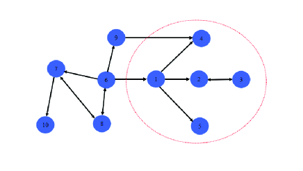
Figure 9: A testing network with 10 nodes, where the part in the red circle is the subnetwork of interest whose topology is to be inferred.

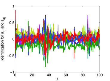
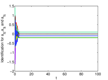
Figure 10: Topology inference of a subnetwork. Left: time evolution of $\hat{a}_{ij}(i=1,4,j=1,2,\cdots,5)$; right: $\hat{a}_{ij}(i=2,3,5,j=1,2,\cdots,5)$.

In this section, numerical examples are presented to illustrate the effectiveness of the proposed identification schemes. Several benchmark chaotic systems, such as Lü system, Chua’s circuit, Duffing system and hyperchaotic Lü system, will be taken as node dynamics. In fact, the well-known Lü system and Chua circuit are respectively simplified models of several three dimensional physical systems, each of them having a chaotic attractor with appropriate system parameters. Moreover, Lü system is a special case of the unified chaotic system, which was proposed by Lü et al. in 2002 [43]. The unified chaotic system is described by

$$\dot{\mathbf{x}}_{i}=\left(\begin{array}[]{ccc}(25\theta+10)(x_{i2}-x_{i1})\\ (28-35\theta)x_{i1}-x_{i1}x_{i3}+(29\theta-1)x_{i2}\\ x_{i1}x_{i2}-\frac{\theta+8}{3}x_{i3}\end{array}\right),$$ (15)

where $\theta\in[0,1]$. When $\theta=0.8$, system (15) is the Lü system, and it reduces to the Lorenz system [44] when $\theta=0$ and Chen system [45] when $\theta=1$. Chua’s circuit [46] can be described as

$$\mathbf{\dot{x}}_{i}=\left(\begin{array}[]{ccc}\zeta(-x_{i1}+x_{i2}-l(x_{i1}))\\ x_{i1}-x_{i2}+x_{i3}\\ -\varrho x_{i2}\end{array}\right),$$ (16)

where $l(x_{i1})=bx_{i1}+\frac{a-b}{2}(|x_{i1}+1|-|x_{i1}-1|)$ is a piecewise-linear function. It has a typical double-scroll chaotic attractor for $\zeta=10,\varrho=18,a=-4/3$ and $b=-3/4$.

Duffing system is a typical two-dimensional chaotic system, as represented by

$$\dot{\mathbf{x}}_{i}=\left(\begin{array}[]{ccc}x_{i2}\\ -p_{2}x_{i1}-p_{3}x_{i1}^{3}-p_{1}x_{i2}+q\cos\omega t\end{array}\right).$$ (17)

It has a chaotic attractor when $p_{1}=0.4,p_{2}=-1.1,p_{3}=2,q=0.6$ and $\omega=1.8$.

There are many hyperchaotic systems emerging in the high dimensional social and economical systems. With high capacity, high security and high efficiency, hyperchaotic systems have been broadly used in secure communications, nonlinear circuits, biological systems and so on. Hyperchaotic Lü system is a typical example of high dimensional chaotic systems, which is described by

$$\dot{\mathbf{x}}_{i}=\left(\begin{array}[]{ccc}a(x_{i2}-x_{i1})+x_{i4}\\ -x_{i1}x_{i3}+cx_{i2}\\ x_{i1}x_{i2}-bx_{i3}\\ x_{i1}x_{i3}+dx_{i4}\end{array}\right).$$ (18)

When $a=36,b=3,c=20$, system (18) has a hyperchaotic attractor for $-0.35<d\leq 1.30$, a chaotic attractor for $-0.46<d\leq-0.35$, and a periodic orbit for $-1.03<d\leq-0.46$.

In what follows, a classical five-node directed network is employed as the underlying testing network. The weighted coupling matrix is described as

$$A=\rho\left(\begin{array}[]{ccccc}0&0&0&0&0\\ 1&-2&1&0&0\\ 0&1&-1&0&0\\ 1&0&0&-1&0\\ 1&0&0&0&-1\end{array}\right),$$

where $\rho$ is the coupling strength, which is supposed to be 0.1 in the following simulations.

The stochastic differential delay equations are numerically solved employing the fourth-order Runge-Kutta method. The stochastic perturbations are randomly assigned and initial values of all the variables are set to be zeros. For brevity, the coupling delay is assumed to be 0.5, and the inner coupling matrix $H$ is supposed to be an identity matrix with a proper dimension. The noise intensity function is assumed to be $\psi_{i}(t)=0.1diag(e_{i1}(t),e_{i2}(t),\cdots,e_{in}(t)),i=1,2,\dots,N$, then one has $\psi_{i}^{T}(t)\psi_{i}(t)=0.01diag({e_{i1}^{2}(t),e_{i2}^{2}(t),\cdots,e_{in}^{2}(t)}).$ Therefore, one further obtains $\mbox{trace}(\psi_{i}^{T}(t)\psi_{i}(t))=0.01\Sigma_{j=1}^{n}e_{ij}^{2}(t)=0.01\mathbf{e}_{i}^{T}(t)\mathbf{e}_{i}(t)$, which satisfies Assumption 3.2. The identification error and synchronization error are defined as $E_{1}(t)=\sum\limits_{i=1}^{N}\sum\limits_{j=1}^{N}|\hat{a}_{ij}-a_{ij}|/N^{2}$ and $E_{2}(t)=\sum\limits_{i=1}^{N}\|\mathbf{e}_{i}(t)\|_{1}/N$, respectively, where $\|\cdot\|_{1}$ represents 1-norm.

$\mathbf{Example4.1}$ Consider the Lü system as node dynamics in the drive network layer, and the Chua’s circuit as node dynamics in the response layer. It is obvious that Assumption 3.1 is satisfied [47]. The map $\phi_{i}$ is taken as $\mathbf{y}_{i}(t)=\phi_{i}(\mathbf{x}_{i}(t))=(2x_{i1},x_{i2},\frac{1}{2}x_{i3}^{2})$, then

$$D\phi_{i}(\mathbf{x}_{i})=\left(\begin{array}[]{ccc}2&0&0\\ 0&1&0\\ 0&0&x_{i3}\end{array}\right).$$

The adaptive controllers and updating laws are designed according to (6)-(8), with parameters being $k_{i}=30,\delta_{ij}=20$.

Figures 2-4 present successful identification results upon generalized synchronization. Identification error is displayed in the left panel of Fig. 2, which illustrates that the underlying topology of the drive network layer (1) is correctly inferred by the proposed control technique. The right panel of Fig. 2 presents time evolution of the generalized synchronization error, which goes to zero rapidly. The left panel of Fig. 2 gives time evolution of $\hat{a}_{ij}~{}(i,j=1,2,...,5)$. To have a clearer view, estimation of incoming edges of node 2 is given in the right panel. It is obvious that two curves corresponding to $\hat{a}_{21}$ and $\hat{a}_{23}$ get stabilized at 0.1, two curves corresponding to $\hat{a}_{24}$ and $\hat{a}_{25}$ stabilize at 0, and the curve $\hat{a}_{22}$ goes to $-0.2$. Figure 4 shows the phase diagrams of node 2 in the two-layer Lü-Chua network. One can see that the two attractors are similar in a certain mode. Furthermore, the relationship between counterparts in the two network layers is examined. The left panel of Fig. 4 shows $x_{i3}$ and $y_{i3}$ of node 2 in the two layers, where the transients are discarded. The relationship is in accord with the predefined generalized outer synchronization manifold $y_{i3}=\frac{1}{2}x_{i3}^{2}$. The right panel of Fig. 4 displays the time-varying adaptive feedback gains $d_{i}(t)~{}(i=1,2,...,5)$. It is seen that the adaptive feedback gains stabilize at some constants upon successful topology identification. Figure 5 displays the time evolution of the component variables $x_{i3}~{}(i=1,2,...,5)$ of nodes in the drive layer for this successful identification case. For a clearer view, the time axis is restricted to the interval [0,10]. It is obvious that the trajectories are asynchronous.

It is well-known that the linear independence condition in Assumption 3.3 is a very essential condition for guaranteeing successful topology identification. Just as mentioned in Remark 3.4, synchronization in the unknown network will make the linearly independence condition unsatisfied, which further leads to topology identification failure. In the case of identification failure, we usually start with checking whether nodes of the unknown network achieve some kind of synchronization, since this is more feasible and practical than checking the linear independence condition. This statement can be clearly illustrated by Figs. 5 and 6. Figure 5 illustrates that for successful topology identification, nodes are asynchronous. Figure 6 displays the identification results for $a_{ij}~{}(i,j=1,2,...,5)$ and time evolution of the component variables $x_{i3}~{}(i=1,2,...,5)$ in the drive layer of the two-layer Lü-Chua network for $\rho=5$ and $\tau=0.01$. From the left panel, it is observed that although $\hat{a}_{ij}$ get stabilized, they do not arrive at the expected values. The reason can be explained from the right panel, where the component variables $x_{i3}$ of each node in the unknown network layer run into synchronization, which directly leads to the failure of topology identification. That is to say, synchronization hinders topology identification.

$\mathbf{Example4.2}$ Take the hyperchaotic Lü system as node dynamics in the drive network layer, and the Duffing system as node dynamics in the response layer. The generalized synchronization map $\phi_{i}$ is supposed to be $\mathbf{y}_{i}(t)=\phi_{i}(\mathbf{x}_{i}(t))=(x_{i1}+2x_{i2},\frac{1}{2}x_{i3}+x_{i4})$, then

$$D\phi_{i}(\mathbf{x}_{i})=\left(\begin{array}[]{cccc}1&0&2&0\\ 0&\frac{1}{2}&0&1\end{array}\right).$$

The adaptive controllers and updating laws are designed accordingly.

Figure 8 displays identification error and synchronization error of the two-layer hyperchaotic Lü-Duffing network. It is obvious that the topological structures of the drive layer is successfully inferred and two layers reach predefined generalized outer synchronization. Fig. 8 shows estimation for ${a}_{ij}~{}(i,j=1,2,...,5)$ and time evolution of adaptive feedback gains $d_{i}~{}(i=1,2,...,5)$. It can be seen that after transient oscillations, $\hat{a}_{ij}$ get stabilized at ${a}_{ij}$. Meanwhile, as can be obtained from the proof, the adaptive feedback gains stabilize at constants.

From this example, one can see that the proposed technique can be employed to infer unknown topologies of complex networks composed of systems with high dimensions and complicated dynamics by constructing auxiliary networks composed of simpler systems. From this viewpoint, the proposed technique can greatly simplify practical design.

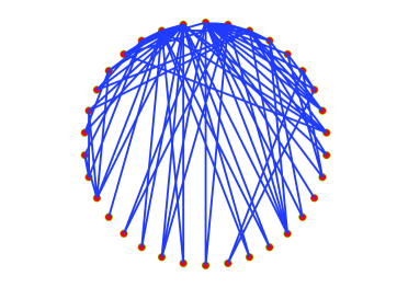
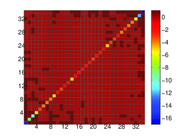
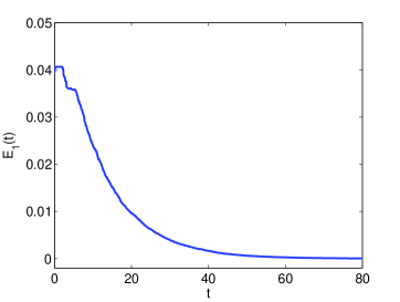
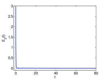
Figure 11: The model of the Zachary Karate Club network (left) and the colormap of the recovered unweighted coupling matrix (right).

Figure 12: Identification error (left) and synchronization error (right) of the Zachary Karate Club network.

$\mathbf{Example4.3}$ This method can also be employed to infer connections in a subnetwork that is embedded within a complex system. For simplicity, the network consisting of 10 unidirectionally connected nodes, as shown in Fig. 9, is considered. Assume that our interest is to infer the topology of the subnetwork composed of nodes 1 to 5 and each node’s dynamical behavior can be monitored. Nodes 1 and 4 are directly influenced by the hidden nodes 6 and 9, respectively. To infer the topology of this subnetwork, an auxiliary network consisting of five nodes is constructed. Let node dynamics of the interested 5-node subnetwork be the Lü system, and Chua’s circuit as node dynamics of the auxiliary one. Controllers and updating laws are designed according to (6)-(8), where system parameters and the map $\phi_{i}$ are supposed to be the same as those in Example 1.

Figure 10 displays estimation for ${a}_{ij}~{}(i,j=1,2,\cdots,5)$. It is shown that in the left panel, $\hat{a}_{1j}$ and $\hat{a}_{4j}$ are oscillating, while in the right panel, $\hat{a}_{2j},\hat{a}_{3j}$ and $\hat{a}_{5j}$ get stabilized at proper constants that are the exact corresponding values of ${a}_{2j},{a}_{3j}$ and ${a}_{5j}$. This figure illustrates that the incoming links of nodes which are free of latent disturbances can be successfully inferred, while nodes that they are directly disturbed by hidden sources cannot be identified and their estimation will oscillate accordingly. Therefore, the method can be applied to infer topology of a subnetwork as well as locate the immediate neighbors of hidden sources.

$\mathbf{Example4.4}$ Consider the well-known Zachary Karate Club network [48] as the testing network, which has 34 nodes and 78 edges, with the topology structure being displayed in the left panel of Fig. 11. For brevity, take $\phi_{i}$ as a linear map in the numerical simulation, which is supposed to be $\mathbf{y}_{i}(t)=\phi_{i}(\mathbf{x}_{i}(t))=(2x_{i1},x_{i2},x_{i3}+1)$, then

$$D\phi_{i}(\mathbf{x}_{i})=\left(\begin{array}[]{ccc}2&0&0\\ 0&1&0\\ 0&0&1\end{array}\right).$$

The coupling strength $\rho$ of the unknown coupling matrix is supposed to be 0.01, and the coupling delay is 2. Adaptive controllers and updating laws are designed according to (6)-(8), and the parameters $k_{i}$ in (8) are taken as 100. Other parameters are designed as the same as those in Example 4.1. The right panel of Fig. 11 presents the the colormap of the recovered unweighted coupling matrix. Figure 12 gives the identification error and synchronization error. It can be obtained that the unknown topology of the testing Zachary Karate Club network has been correctly recovered, and the drive layer achieves generalized synchronization with the constructed response layer. This further illustrates the effectiveness of the proposed method.

5 Conclusions

Topology identification of complex dynamical networks containing communication delay has been investigated via driving-based generalized synchronization of two-layer networks. An adaptive control technique has been proposed to infer the underlying topology of a dynamical network by constructing an auxiliary layer consisting of an identical number of systems. The auxiliary layer is driven by signals from the unknown network so that it reaches generalized outer synchronization with the drive layer and successful topology identification is achieved in the sense of mean square. Since perturbations caused by control input have been taken into consideration, the proposed method is comparatively more practical than previous results. The main theorem contains some recent results as special cases. Numerical simulations have been performed to illustrate the effectiveness of the proposed adaptive identification strategies. Particularly, when the considered network is composed of systems with high-dimension or complicated dynamics, a much simpler auxiliary layer can be constructed for the purpose of topology inference. Moreover, it has been shown that method can be applied to infer topology of a subnetwork embedded within a network and locate hidden sources. Our results provide engineers with certain theoretical supports and guidance for monitoring network structures as well as locating hidden sources. We expect that our analysis could prompt attention and provide basic insight into further research endeavors on understanding practical and economical topology identification.

6 Acknowledgments

This work was supported by the National Natural Science Foundation of China under Grants 61573252 and 61203159, the Fundamental Research Funds for the Central Universities under Grant 2014201020206, and the Youth Fund Project of the Humanities and Social Science Research for the Ministry of Education of China under Grant 14YJCZH173.

References

- [1] Watts D J and Strogatz S H 1998 Nature 393 440–442
- [2] Barabási A L and Albert R 1999 Science 286 509–512
- [3] Liu C, Liu J and Jiang Z 2014 IEEE Transactions on Cybernetics 44 2274–2287
- [4] Sheshbolouki A, Zarei M and Sarbazi-Azad H 2015 Journal of Statistical Mechanics: Theory and Experiment 2015 P10022
- [5] Newman M E J 2003 SIAM Review 45 167–256
- [6] Boccaletti S, Latora V, Moreno Y, Chavez M and Hwang D U 2006 Physics Reports 424 175–308
- [7] Zhou J and Lu J a 2007 Physica A 386 481–491
- [8] Wu X 2008 Physica A 387 997–1008
- [9] Liu H, Lu J A, Lü J and Hill D J 2009 Automatica 45 1799–1807
- [10] Zhao J, Li Q, Lu J A and Jiang Z P 2010 Chaos 20 023119
- [11] Wu Z and Fu X 2013 IET Control Theory and Applications 7 1269–1275
- [12] Wang W X, Yang R, Lai Y C, Kovanis V and Grebogi C 2011 Physical Review Letters 106 154101
- [13] Jansen R, Yu H, Greenbaum D, Kluger Y, Krogan N J, Chung S, Emili A, Snyder M, Greenblatt J F and Gerstein M 2003 Science 302 449–453
- [14] Marwan N, Romano M C, Thiel M and Kurths J 2007 Physics Reports 438 237–329
- [15] Romano M C, Thiel M, Kurths J and Grebogi C 2007 Physical Review E 76 036211
- [16] Wu X, Zhou C, Chen G and Lu J a 2011 Chaos 21 043129
- [17] Wu X, Wang W and Zheng W X 2012 Physical Review E 86 046106
- [18] Nabi-Abdolyousefi M and Mesbahi M 2012 IEEE Transactions on Automatic Control 57 3214–3219
- [19] Li D, Han M and Wang J 2012 IEEE Transactions on Neural Networks and Learning Systems 23 787–799
- [20] Li C, Sun W and Kurths J 2007 Physical Review E 76 046204
- [21] Tang H, Chen L, Lu J a and Chi K T 2008 Physica A: Statistical Mechanics and its Applications 387 5623–5630
- [22] Wu Z and Fu X 2012 Nonlinear Dynamics 69 685–692
- [23] Wu X, Zheng W X and Zhou J 2009 Chaos 19 013109
- [24] Kocarev L and Parlitz U 1996 Physical Review Letters 76 1816
- [25] Juan M and Xingyuan W 2008 Chaos: An Interdisciplinary Journal of Nonlinear Science 18 023108
- [26] Senthilkumar D, Lakshmanan M and Kurths J 2008 Chaos: An Interdisciplinary Journal of Nonlinear Science 18 023118
- [27] Koronovskii A, Moskalenko O and Hramov A 2012 Technical Physics Letters 38 924–927
- [28] Yang X and Cao J 2009 Physics Letters A 373 3259–3272
- [29] Paulsson J 2004 Nature 427 415–418
- [30] Raser J M and O’Shea E K 2005 Science 309 2010–2013
- [31] Chen C P, Liu Y J and Wen G X 2014 IEEE Transactions on Cybernetics 44 583–593
- [32] Guo Z, Wang J and Yan Z 2014 Neural Networks 54 112–122
- [33] Cao J and Wang J 2005 IEEE Transactions on Circuits and Systems I: Regular Papers 52 417–426
- [34] Wei X, Wu X, Lu J a and Zhao J 2015 Journal of Statistical Mechanics: Theory and Experiment 2015 P11021
- [35] Gomez S, Diaz-Guilera A, Gomez-Gardeñes J, Perez-Vicente C J, Moreno Y and Arenas A 2013 Physical Review Letters 110 028701
- [36] Mao X 2002 Journal of Mathematical Analysis and Applications 268 125–142
- [37] Lu J and Cao J 2007 Physica A 382 672–682
- [38] Lu J, Kurths J, Cao J, Mahdavi N and Huang C 2012 IEEE Transactions on Neural Networks and Learning Systems 23 285–292
- [39] Yang X, Cao J, Long Y and Rui W 2010 IEEE Transactions on Neural Networks 21 1656–1667
- [40] Yu D and Parlitz U 2011 Plos One 6 e24333
- [41] Chen L, Lu J a and Tse C K 2009 IEEE Transactions on Circuits and Systems II: Express Briefs 56 310–314
- [42] Zhang S, Wu X, Lu J A, Feng H and Lu J 2014 IEEE Transactions on Circuits and Systems I: Regular Papers 61 3216–3224
- [43] Lü J, Chen G, Cheng D and Celikovsky S 2002 International Journal of Bifurcation and Chaos 12 2917–2926
- [44] Lorenz E N 1963 Journal of the Atmospheric Sciences 20 130–141
- [45] Chen G and Ueta T 1999 International Journal of Bifurcation and Chaos 9 1465–1466
- [46] Chua L O 1992 Archiv fur Elektronik and Ubertragung stechnik 46 250–257
- [47] Li D, Lu J a, Wu X and Chen G 2006 Journal of Mathematical Analysis and Applications 323 844–853
- [48] Zachary W W 1977 Journal of Anthropological Research 33 452–473