Approximation algorithms for the two-center problem of convex polygon

Abstract

Given a convex polygon $P$ with $n$ vertices, the two-center problem is to find two congruent closed disks of minimum radius such that they completely cover $P$. We propose an algorithm for this problem in the streaming setup, where the input stream is the vertices of the polygon in clockwise order. It produces a radius $r$ satisfying $r\leq 2r_{opt}$ using $O(1)$ space, where $r_{opt}$ is the optimum solution. Next, we show that in non-streaming setup, we can improve the approximation factor by $r\leq 1.84r_{opt}$, maintaining the time complexity of the algorithm to $O(n)$, and using $O(1)$ extra space in addition to the space required for storing the input.

Keywords. Computational geometry, two-center problem, lower bound, approximation algorithm, streaming algorithm.

1 Introduction

Covering a geometric object (e.g., a point set or a polygon) by disks has drawn a lot of interest to the researchers due to its several applications, for example, base station placement in mobile network, facility location in city planning, etc. There are mainly two variations of the disk cover problem, namely standard version and discrete version, depending on the position of the centers of the disks to be placed. In standard version, the position of centers of disks are anywhere on the plane, whereas in the discrete version, the center of the disks must be on some specified points, also given as input. The objective of a $k$-center problem for a given set of points $S$ in a metric space is to find out $k$ points (also called centers) $c_{1},c_{2},\ldots,c_{k}$ in the underlying space so that the largest distance of a point $p\in S$ from its nearest center $c\in\{c_{1},c_{2},\ldots,c_{k}\}$ is minimized. In other words, in $k$-center problem we want to cover a set of points using $k$ congruent balls of minimum radius. In this paper, we consider the standard two-center problem for a convex polygon $P$ in the $L_{2}$ metric, where the objective is to identify centers of two congruent closed disks whose union completely covers the polygon $P$ and their (common) radius $r$ is minimum. As stated by Kim and Shin [13], the major difference between the two-center problem for a convex polygon $P$ and the two-center problem for a point set $S$ are (1) points covered by the two disks in the former problem are in convex positions (instead of arbitrary positions), and (2) the union of two disks should also cover the edges of the polygon $P$. The feature (1) indicates the problem is easier than the standard two-center problem for points, but feature (2) says that it might be more difficult.

1.1 Related work

The $k$-center problem, where $S$ is a set of points in a Euclidean plane and the distance function is the $L_{2}$ metric, is NP-complete for any dimension $d\geq 2$ [14]. Therefore it makes sense to study the $k$-center problem for small (fixed) values of $k$ ([3, 4, 7, 9, 10, 11, 18]) and to search for efficient approximation algorithms and heuristics for the general version ([10], [16]). Hershberger [9] proposed an $O(n^{2}\log n)$ time algorithm for the standard version of the two-center problem for the $n$-points in plane. Sharir [18] improved the time complexity of the problem to $O(n\log^{9}n)$. Eppstein [7] proposed a randomized algorithm with expected time complexity $O(n\log^{2}n)$. Later, Chan [4] proposed two algorithms for this problem. The first one is a randomized algorithm that runs in $O(n\log^{2}n)$ time with high probability, and the second one is a deterministic algorithm that runs in $O(n\log^{2}n(\log\log n)^{2})$ time. The discrete version of the two-center problem for a point set was solved by Agarwal et al. [2] in $O(n^{4/3}\log^{5}n)$ time. The standard and discrete versions of the two-center problem for a convex polygon $P$ was first solved by Kim and Shin [13] in $O(n\log^{3}n\log\log n)$ and $O(n\log^{2}n)$ time respectively, where $n$ is the number of vertices of $P$. Recently Vigan [19] proposed the problem of covering a simple polygon by $k$ geodesic disks whose centers lie inside $P$. Here, the geodesic distance between a pair of points $s$ and $t$ inside the polygon is the length of the shortest $s-t$ path inside $P$. He showed that the maximum radius among these $k$ geodesic disks is at most twice as large as that of an optimal solution, and the time complexity of the proposed algorithm is $O(k^{2}(n+k)\log(n+k))$. The algorithm proposed by Vigan [19], if applied for convex polygon, the approximation factor remains unaltered. There exists a heuristic to cover a convex region by $k$ congruent disks of minimum radii [6]. However, to the best of our knowledge there are no linear time approximation algorithm for the $k$-center problem of a convex polygon, where $k\geq 2$.

In the streaming model, McCutchen et al. [15] and Guha [8] have designed a ($2+\epsilon$)-approximation algorithm for the $k$-center problem of a point set in $\mathbb{R}^{d}$ using $O(\frac{kd}{\epsilon}\log(\frac{1}{\epsilon}))$ space. For the 1-center problem, Agarwal and Sharathkumar [1] suggested a $((1+\sqrt{3})/2+\epsilon)$-factor approximation algorithm using $O(\frac{d}{\epsilon^{3}}\log(\frac{1}{\epsilon}))$ space. The approximation factor was later improved to $1.22$ by Chan and Pathak [5]. Recently, Kim and Ahn [12] proposed a ($1.8+\epsilon$)-approximation algorithm for the two-center problem of a point set in $\mathbb{R}^{2}$. It uses $O(\frac{d}{\epsilon})$ space and update time where insertion and deletion of the points in the set are allowable. To the best of our knowledge, there is no approximation result for the two-center problem for a convex polygon under the streaming model.

1.2 Our result

We propose a $2$-factor approximation algorithm for the two-center problem of a convex polygon in streaming setup. Here, the vertices of the input polygon is read in clockwise manner and the execution needs $O(n)$ time using $O(1)$ space. Next we show that if the restriction on streaming model is relaxed, then we can improve the approximation factor to 1.84 maintaining the time complexity to $O(n)$ and using $O(1)$ extra space apart from the space required for storing the input. We have observed the fact that if two disks cover a convex polygon $P$, then they must also cover a “line segment” or a “triangle” lying inside that polygon $P$. This fact has been used in our work to analyze the approximation factor of the radius of disks.

1.3 Notations and terminologies used

Throughout the paper we use the following notations. The line segment joining any two points $p$ and $q$ is denoted by $\overline{pq}$ and its length is denoted by $|{pq}|$. The $x$- and $y$-coordinate of a point $p$ are denoted by $x(p)$ and $y(p)$ respectively. The “horizontal distance” between a pair of points $p$ and $q$ is $|x(p)-x(q)|$ (the absolute difference between their $x$-coordinates). Similarly, the “vertical distance” between a pair of points $p$ and $q$ is $|y(p)-y(q)|$. The notation $s\in\overline{pq}$ implies that the point $t$ lies on $\overline{pq}$. We will use $\triangle$, $\Box$ and $\Diamond$ to represent triangle, axis-parallel rectangle, and quadrilateral of arbitrary orientation of edges respectively.

1.4 Organization of the paper

In this paper, the Section 2 describes the algorithm for two-center problem of a convex polygon in streaming setup along with the detailed analysis of the approximation factor. Section 3 discusses the same problem under non-streaming model and a linear time algorithm is proposed along with a detailed discussion on the analysis of approximation factor. Finally we conclude in section 4 with future work.

2 Two-center problem for convex polygon under streaming model

In this section, we first describe the streaming algorithm for the problem in subsection 2.1. Then in subsection 2.2, we discuss about the type of lower bounds of the optimal radius of the disks followed by the interesting characteristic of the problem in subsection 2.3 which shows that only quadrilaterals, triangles are to be studied instead of all convex polygons for the approximation factor. Subsection 2.4 will show the detailed analysis of the approximation factor.

2.1 Proposed algorithm

Under the streaming data model, the algorithm has only a limited amount of working space. So it cannot store all the input items received so far. In this model, the input data is read only once in a single pass. It does not require the entire data set to be stored in memory. In the streaming setup, the vertices of the convex polygon $P$ arrives in order one at a time. In a linear scan among the vertices of $P$, we can identify the four vertices $a$, $b$, $c$ and $d$ of the polygon $P$ with minimum $x$-, maximum $x$-, minimum $y$- and maximum $y$-coordinate respectively as shown in Figure 1(a). This needs $O(1)$ scalar locations. Let $\mathcal{R}=\Box efgh$ be an axis-parallel rectangle whose four sides passes through the vertices $a,b,c$ and $d$ of the convex polygon $P$, where $a\in\overline{gh}$, $b\in\overline{he}$, $c\in\overline{ef}$ and $d\in\overline{fg}$.

Figure 1: (a) Covering rectangle ${\cal R}=\Box efgh$ for the convex polygon $P$. (b) Rectangle ${\cal R}$ of size $L\times W$ covered by two disks $C_{1}$ and $C_{2}$

The length and width of rectangle $\mathcal{R}$ are $L=|x(c)-x(a)|$ and $W=|y(b)-y(d)|$ respectively. We split $\mathcal{R}$ into two equal parts ${\cal R}_{1}$ and ${\cal R}_{2}$ by a vertical line $\overline{v_{1}v_{2}}$, where $v_{1}\in\overline{eh}$ and $v_{2}\in\overline{fg}$ (see Figure 1(a)). Finally, compute two congruent disks $C_{1}$ and $C_{2}$ of minimum radii circumscribing ${\cal R}_{1}$ and ${\cal R}_{2}$ respectively (see Figure 1(b)). The output of our algorithm is $r$, the radii of $C_{1}$ (resp. $C_{2}$). Since the two disks cover the rectangle $\mathcal{R}$ together, they must also cover the polygon $P$ lying inside $\mathcal{R}$. For an axis-parallel rectangle ${\mathcal{R}}=\Box{efgh}$ of length $L$ and width $W$ (where $0<W\leq L$) covering the polygon $P$, the value of $r$ (as shown in Figure 1(b)) computed by our algorithm is

$$r=\sqrt{\left(\frac{L}{4}\right)^{2}+\left(\frac{W}{2}\right)^{2}}=\frac{1}{4}\sqrt{L^{2}+4W^{2}}$$ (1)

The time complexity of our algorithm, determined mainly by identification of the four vertices $a$, $b$, $c$ and $d$ during the streaming input of the vertices of $P$, takes $O(n)$ time, where $n$ is the size of the input.

Let $r$ be the radius of the two congruent disks $C_{1}$ and $C_{2}$ for enclosing $P$, returned by our algorithm. If $r_{opt}$ is the minimum radius of the two congruent disks that cover $P$, then the approximation factor of our algorithm is $\alpha=\frac{r}{r_{opt}}$. We now propose a lower bound $\rho$ of $r_{opt}$, which suggests an upper bound $\frac{r}{\rho}$ of $\alpha$, i.e. $\alpha\leq\frac{r}{\rho}$.

2.2 Lower bound $\rho$ of $r_{opt}$

Definition 1.

A convex polygon $P$ is said to be exactly covered by an axis-parallel rectangle ${\cal R}$, if $P\cap{\cal R}=P$ and each of the four side of ${\cal R}$ contain at least one vertex of $P$.

Definition 2.

A convex polygon $P_{1}$ is said to be a subpolygon of a convex polygon $P_{2}$, if the set of vertices of $P_{1}$ are subset of the vertices of $P_{2}$ and this is denoted by $P_{1}\subseteq P_{2}$.

The Figure 1(a) shows that the convex polygon $P$ is exactly covered by the rectangle $\cal R$ (Definition 1) and the quadrilateral $\Diamond abcd\subseteq P$ (Definition 2).

Now, to have a better estimate of the approximation factor, we need a lower bound of $r_{opt}$, which is as large as possible. The following observations give us an idea of choosing two types of lower bound of $r_{opt}$.

Observation 1.

The two disks whose union covers the convex polygon $P$, must also cover a convex polygon which is a subpolygon of $P$.

Thus, the lower bound of the radii of the two disks for covering a quadrilateral $\Diamond abcd$, where $\Diamond abcd\subseteq P$, is also a lower bound for the radius of the two-center problem for the convex polygon $P$.

Observation 2.

Let $\mathcal{L}$ be the longest line segment within a quadrilateral $\Diamond abcd$ inside $P$. The two disks whose union covers the convex polygon $P$, must also cover the line segment $\cal L$ because $\Diamond abcd\subseteq P$.

From Observation 2, we conclude that $\rho\geq\frac{{\cal L}}{4}$. Moreover, the length of the line segment $\cal L$ can be at most $D$, the diameter of the convex polygon $P$.

Observation 3.

Let $\Delta$ be a triangle inside the polygon $P$. If a pair of disks $C_{1}$ and $C_{2}$ completely cover $P$, they must also cover the triangle $\Delta$. Again, if a pair of disks $C_{1}$ and $C_{2}$ cover a triangle $\Delta$, one of them must fully cover one of the edges of $\Delta$.

Thus, a lower bound $\rho$ of $r_{opt}$ is half of the length of the smallest edge of a triangle inside $P$ (Observation 3). In order to tighten the lower bound we find a triangle $\Delta$ inside $P$ whose smallest edge is as large as possible. We use $\ell$ to denote the smallest edge of $\Delta$. We also use $\ell$ to denote the length of $\ell$. Thus, ${\ell}/{2}$ is a lower bound for $\rho$.

Note that, in our analysis $\Delta$ may not always be the triangle whose smallest side is of maximum length among all triangles inscribed in $P$. We try to find a triangle $\Delta$ inscribed in $P$ such that the length of its smallest side $\ell$ has a closed form expression in terms of the length ($L$) and width ($W$) of the rectangle $\cal R$ covering $P$. This helps us to establish an upper bound on the approximation factor $\alpha$ of our algorithm.

2.3 Characterization of the problem

The upper bound of the approximation factor $\alpha$ for the two-center problem for the polygon $P$ is $\alpha\leq\frac{r}{({\ell}/{2})}$ or, $\alpha\leq\frac{r}{\left(|{\cal L}|/4\right)}$ depending on the type of lower bound used. In order to have a worst case estimate of the approximation factor, at first we fix $r$ (or in other words both $L$ and $W$ of the rectangle ${\cal R}$). Now, there are different convex polygons exactly covered by the same rectangle $\cal R$, and the lower bound of optimal radius for each such polygon are possibly different. Thus in order to have a worst estimate of the upper bound for the approximation factor $\alpha$, we choose the polygon $P$ inside $\cal R$ for which the lower bound ($\rho$) of $r_{opt}$ is minimum among all possible polygons inside ${\cal R}$. The following observation gives us an intuition for choosing quadrilaterals and triangles instead of inspecting all possible polygons exactly covered by the rectangle $\cal R$.

Observation 4.

Let $P$ be a convex polygon which is exactly covered by an axis-parallel rectangle $\cal R$ of length $L$ and width $W$ ($W\leq L$). Let $\Pi$ be a subpolygon of $P$ ($\Pi\subseteq P$) so that $\Pi$ is also exactly covered by the same axis-parallel rectangle $\cal R$. Then the upper bound of the approximation factor $\alpha$ of our algorithm for polygon $P$ will be smaller than (or equal to) that for polygon $\Pi$.

Proof:   Follows from the Observation 1 that the lower bound $\rho$ ($(\ell/2)$ or $(|{\cal L}|/4)$) of the optimal radius $r_{opt}$ for polygon $\Pi$ will be less than that for polygon $P$ (because of the fact that any triangle $\Delta$ in $\Pi$ or any line segment $\cal L$ in $\Pi$ also lies inside $P$).  $\Box$

Observation 4 says that in order to measure the upper bound of the approximation factor of our algorithm for a given convex polygon $P$, one should choose a quadrilateral $\Diamond abcd$ as a subpolygon $\Pi$ of $P$ (i.e. $\Pi=\Diamond abcd\subseteq P$) where both $P$ and $\Pi=\Diamond abcd$ are exactly covered by the same rectangle $\cal R$. The reason for choosing the quadrilateral $\Diamond abcd$ as subpolygon $\Pi$ of $P$ is that quadrilateral is the minimal convex polygon (“minimal” in the sense that “there exists no subpolygon of the quadrilateral $\Diamond abcd$ which is exactly covered by the same rectangle $\cal R$”). From now onwards, we will use $\Pi$ to denote “a subpolygon of $P$ such that both $P$ and $\Pi$ are exactly covered by the same rectangle $\cal R$”. It needs to mention that, we may have two degenerate cases, (i) if a vertex $p$ of the given convex polygon $P$ coincides with a vertex of $\cal R$, then the minimal subpolygon $\Pi$ of $P$ will be a triangle with one of its vertex at $p$, and (ii) if (maximum-$x$, maximum-$y$), and (minimum-$x$, minimum-$y$) coordinates correspond to two vertices, say $p$ and $q$, of the given convex polygon $P$ (i.e. any two non-adjacent corners, say $e$ and $g$, of the rectangle $\cal R$ coincides with these two vertices $p$ and $q$), then we need to consider diagonal $\overline{eg}$ as a subpolygon $\Pi$ (with area zero). Now note that, whatever be the shape of a convex polygon $P$ that is exactly covered by rectangle $\cal R$, we always obtain a subpolygon $\Pi$ as a quadrilateral $\Diamond abcd\subseteq P$ (including degeneracies). The observation 4 says that the approximation factor for this given convex polygon $P$ will be bounded above by that of its subpolygon $\Pi=\Diamond abcd$. Therefore we will concentrate on all possible quadrilaterals inside $\cal R$ rather than studying convex $n$-gons with $n\geq 5$. Now, each such quadrilaterals have different lower bound of optimal radius. The minimum of these lower bounds for $r_{opt}$ among all possible quadrilaterals will be used to compute the upper bound of the approximation factor for an arbitrary convex polygon which is exactly covered by the rectangle $\cal R$.

In our streaming model we have stored only the four vertices $a$, $b$, $c$ and $d$ of the convex polygon $P$ and we find out either a triangle $\Delta$ (as defined in earlier section), or the longest line segment $\cal L$ inside the $\Diamond abcd$ instead of searching them inside $P$ and the approximation factor thus obtained gives an upper bound for the same in $P$.

In the next subsection, we perform an exhaustive case analysis and finally present a flowchart in Figure 10 to justify the following result.

Theorem 1.

The approximation factor $\alpha$ of the two-center problem for a convex polygon $P$ in the streaming model is $2$.

Proof.

Follows from Lemma 1, 2 and 3, stated in the next subsection. ∎

2.4 Analysis of approximation factor

Let, $h_{1}$, $v_{1}$, $h_{2}$ and $v_{2}$ be the mid-points of $\overline{gh}$, $\overline{he}$, $\overline{ef}$ and $\overline{fg}$ respectively, and $|{fg}|=L$ and $|{ef}|=W$ ($L\geq W$ as shown in Figure 1(b)). Surely, $L\leq D$ (the diameter of the polygon $P$). We study, in detail, the case when $\Pi$ is a quadrilateral. We also discuss the two degenrate cases, namely, (i) $\Pi$ is a triangle and (ii) $\Pi$ is a diagonal $\overline{eg}$ of ${\cal R}=\Box efgh$.

2.4.1 $\Pi$ is a quadrilateral $\Diamond abcd$

We consider the following two cases separately.

Case I: $0<\frac{W}{L}\leq\frac{\sqrt{3}}{2}$

One of the diagonals of $\Diamond abcd$ (e.g. $\overline{ac}$ in Figure 1(a)) must be at least of length $L$ and the two congruent disks must cover this diagonal. Thus, we have $|{\cal L}|\geq L$, and hence $\rho\geq\frac{L}{4}$, implying $\alpha=\frac{r}{\rho}\leq\frac{\frac{1}{4}\sqrt{L^{2}+4W^{2}}}{L/4}=\sqrt{1+4\left(\frac{W}{L}\right)^{2}}$. Since $\left(\frac{W}{L}\right)\leq\frac{\sqrt{3}}{2}$, we have $\alpha\leq 2$.

Figure 2: Demonstration of Observation 5: ($a$) Case ($i$) and ($b$) Case ($ii$).

Case II: $\frac{\sqrt{3}}{2}<\frac{W}{L}\leq 1$

Before studying this case, we show the following two important observations:

Observation 5.

If both the vertices $a$ and $c$ lie at the same side of $\overline{h_{1}h_{2}}$, the approximation factor $\alpha$ will be 2.

Proof:   Without loss of generality, assume that both $a$ and $c$ lie below $\overline{h_{1}h_{2}}$, and $y(a)<y(c)$ as shown in Figure 2. Depending on the position of $b$ on the edge $\overline{eh}$, we consider the following two cases :

Case (i): $b$ lies on $\overline{hv_{1}}$

Refer to Figure 2(a). Choose a point $c^{\prime}\in\overline{gh}$ such that $y(c)=y(c^{\prime})$. Let $q$ be the point of intersection of $\overline{ch}$ and $\overline{c^{\prime}e}$. Whatever be the position of the vertex $b$ on $\overline{hv_{1}}$, the point $q$ must lie always inside the quadrilateral $\Diamond abcd$. Hence, the triangle $\triangle aqc$ will also lie inside the $\Diamond abcd$. Now, as $|ce|\geq\frac{W}{2}$, we have $|cq|=|c^{\prime}q|=\frac{1}{2}|c^{\prime}e|\geq\frac{1}{2}|h_{1}e|=\frac{1}{2}\sqrt{L^{2}+\left(W/2\right)^{2}}$. Here, we choose the triangle $\triangle aqc$. Since the point $a$ lies below $c^{\prime}$, we have $|aq|\geq|c^{\prime}q|=|cq|$. Also, $|ac|\geq L>\frac{1}{2}\sqrt{L^{2}+\left(W/2\right)^{2}}$. Therefore, the smallest side $\ell$ of the triangle $\triangle aqc$ will be at least $\frac{1}{2}\sqrt{L^{2}+\left({W}/{2}\right)^{2}}$. Hence, $\alpha=\frac{r}{\ell/2}=\sqrt{\frac{L^{2}+4W^{2}}{L^{2}+\left({W}/{2}\right)^{2}}}=2\sqrt{\frac{L^{2}+4W^{2}}{4L^{2}+W^{2}}}\leq 2$ (since $W\leq L$).

Case (ii): $b$ lies on $\overline{v_{1}e}$

Refer to Figure 2(b). Consider a horizontal line segment $\overline{z_{1}z_{2}}$ below $\overline{h_{1}h_{2}}$ at a distance of $\frac{W}{8}$. This segment $\overline{z_{1}z_{2}}$ intersects $\overline{gh_{2}}$ at point $q$. Now, since $c\in\overline{h_{2}f}$, $d\in\overline{gf}$ and $b\in\overline{v_{1}e}$, the point $q$ must lie always within $\Diamond abcd$. Hence the triangle $\triangle abq$ will also lie inside $\Diamond abcd$. Here, we choose this triangle $\triangle abq$. Now, $\overline{v_{1}v_{2}}$ intersect $\overline{h_{1}h_{2}}$, $\overline{z_{1}z_{2}}$ and $\overline{gh_{2}}$ at the points $o$, $z_{3}$ and $v_{3}$ respectively, where $|v_{3}v_{2}|=|v_{3}o|=\frac{1}{2}|h_{2}f|=\frac{W}{4}$. From the similar triangles $\triangle gz_{1}q$ and $\triangle v_{3}z_{3}q$, we have

$$\frac{|z_{1}g|}{|z_{3}v_{3}|}=\frac{|z_{1}q|}{|z_{3}q|}$$ (2)

Now, $|z_{1}g|=W-\left(\frac{W}{2}+\frac{W}{8}\right)=\frac{3W}{8}$, $|z_{3}v_{3}|=|v_{3}o|-|z_{3}o|=\left(\frac{W}{4}-\frac{W}{8}\right)=\frac{W}{8}$ and $|z_{1}q|=|z_{1}z_{3}|+|z_{3}q|=\frac{L}{2}+|z_{3}q|$. Hence, the Equation 2 gives $|z_{3}q|=\frac{L}{4}$. Now, in $\triangle abq$, $|aq|\geq|z_{1}q|=\left(|z_{1}z_{3}|+|z_{3}q|\right)=\frac{3L}{4}$, $|bq|\geq\left(\frac{W}{2}+\frac{W}{8}\right)=\frac{5W}{8}$ and $|ab|\geq\sqrt{\left(\frac{L}{2}\right)^{2}+\left(\frac{W}{2}\right)^{2}}$. Since $L\geq W$, we have $\sqrt{\left(\frac{L}{2}\right)^{2}+\left(\frac{W}{2}\right)^{2}}\geq\sqrt{\left(\frac{W}{2}\right)^{2}+\left(\frac{W}{2}\right)^{2}}=0.707W>\frac{5W}{8}$. Also, $\frac{3L}{4}\geq\frac{5W}{8}$, because $L\geq W$. Therefore, the smallest side $\ell$ of the $\triangle abq$ must be at least $\frac{5W}{8}$. Therefore, the approximation factor $\alpha$ will be given by $\alpha=\frac{r}{\ell/2}=\frac{\frac{1}{4}\sqrt{L^{2}+4W^{2}}}{5W/16}=\frac{4}{5}\sqrt{4+\left(L/W\right)^{2}}<\frac{4}{5}\sqrt{4+\left(4/3\right)}$ since $\frac{L}{W}<\frac{2}{\sqrt{3}}$ ($\because\frac{\sqrt{3}}{2}<\frac{W}{L}\leq 1$). Thus, we have $\alpha=\frac{16}{5\sqrt{3}}<2$.  $\Box$

Figure 3: Demonstration of Observation 6: ($a$) Case ($i$) and ($b$) Case ($ii$).

Observation 6.

If both the vertices $b$ and $d$ lie at the same side of $\overline{v_{1}v_{2}}$, the approximation factor $\alpha$ will be 2.

Proof:   Without loss of generality, assume that $b$ and $d$ lie to the right of $\overline{v_{2}v_{1}}$ and $x(d)\geq x(b)$ as shown in Figure 3. Depending on the position of $a$ on the edge $\overline{gh}$, we study the following two cases:

Case (i): $a$ lies on $\overline{gh_{1}}$

Refer to Figure 3(a). Let $b^{\prime}$ be a point on edge $\overline{fg}$ with $x(b^{\prime})=x(b)$. The line segments $\overline{bg}$ and $\overline{b^{\prime}h}$ intersect at $q$. Whatever be the position of $a$ on $\overline{gh_{1}}$, the point $q$ must lie inside the quadrilateral $\Diamond abcd$. Hence, the triangle $\triangle bqd$, as shown in Figure 3(a), must also lie inside $\Diamond abcd$. Here, we choose the triangle $\triangle bqd$. Now, since $|bh|\geq\frac{L}{2}$, we have $|bq|=\frac{1}{2}|bg|\geq\frac{1}{2}|v_{1}g|=\frac{1}{2}\sqrt{W^{2}+\left(\frac{L}{2}\right)^{2}}$. Surely, $|qd|\geq|b^{\prime}q|=|bq|$. Also, $|bd|\geq|{bb^{\prime}}|=W$. Thus the smallest side $\ell$ of triangle $\triangle bqd$ will be either $\overline{bq}$ or $\overline{bd}$. Now,

$\bullet$

if $|bd|\leq|bq|$, we have $\ell=|bd|\geq W$. Therefore, $\alpha=\frac{r}{\ell/2}\leq\frac{1}{2}\sqrt{4+(L/W)^{2}}$. Since $\frac{W}{L}>\frac{\sqrt{3}}{2}$, we have $\alpha\leq\frac{1}{2}\sqrt{4+(4/3)}<2$.

$\bullet$

if $|bd|>|bq|$, we have $\ell=|bq|\geq\frac{1}{2}\sqrt{W^{2}+\left(L/2\right)^{2}}$. Hence $\alpha=\frac{r}{\left(\ell/2\right)}\leq\sqrt{\frac{L^{2}+4W^{2}}{W^{2}+\left(L/2\right)^{2}}}=2$.

Case (ii): $a$ lies on $\overline{h_{1}h}$

Refer to Figure 3(b). Consider a vertical line segment $\overline{z_{1}z_{2}}$ to the right of $\overline{v_{2}v_{1}}$ at a distance of $\frac{L}{8}$. This segment $\overline{z_{1}z_{2}}$ intersect $\overline{v_{1}f}$ at $q$. Now, since $a\in\overline{h_{1}h}$, $b\in\overline{v_{1}e}$ and $c\in\overline{ef}$, the point $q$ must always lie within $\Diamond abcd$. Hence the triangle $\triangle adq$ will also lie inside $\Diamond abcd$. We choose this triangle $\triangle adq$. Now, $\overline{h_{1}h_{2}}$ intersect $\overline{z_{1}z_{2}}$ and $\overline{v_{1}f}$ at the points $h_{3}$ and $h_{4}$ respectively, where $|h_{4}h_{2}|=|h_{4}o|=\frac{1}{2}|v_{1}e|=\frac{L}{4}$, where $o$ is the mid-point of $\overline{h_{1}h_{2}}$. From the similar triangles $\triangle z_{2}fq$ and $\triangle h_{3}h_{4}q$, we have

$$\frac{|z_{2}q|}{|z_{2}f|}=\frac{|h_{3}q|}{|h_{3}h_{4}|}$$ (3)

Now, $|z_{2}q|=|h_{3}q|+\frac{W}{2}$, $|z_{2}f|=L-\left(\frac{L}{2}+\frac{L}{8}\right)=\frac{3L}{8}$ and $|h_{3}h_{4}|=\left(\frac{L}{4}-\frac{L}{8}\right)=\frac{L}{8}$. Thus, Equation 3 gives $|h_{3}q|=\frac{W}{4}$. Now, in $\triangle adq$, $|aq|\geq|h_{1}h_{3}|=\frac{5L}{8}$, $|qd|\geq|z_{2}q|=\frac{3W}{4}$ and $|ad|\geq\sqrt{\left(\frac{L}{2}\right)^{2}+\left(\frac{W}{2}\right)^{2}}$. Any one of the three sides of $\triangle aqd$ can be smallest side $\ell$. Now,

$\bullet$

if $\ell=|qd|\geq\frac{3W}{4}$, we have $\alpha=\frac{r}{\ell/2}\leq\frac{\frac{1}{4}\sqrt{L^{2}+4W^{2}}}{\frac{3W}{8}}=\frac{2}{3}\sqrt{4+(L/W)^{2}}$. Since $\left(\frac{L}{W}\right)\leq\frac{2}{\sqrt{3}}$, we have $\alpha\leq\frac{2}{3}\sqrt{4+(4/3)}=\frac{8}{3\sqrt{3}}<2$.

$\bullet$

if $\ell=|aq|\geq\frac{5L}{8}$, we have $\alpha=\frac{r}{\left(\ell/2\right)}\leq\frac{4}{5}\sqrt{1+4\left(W/L\right)^{2}}\leq\frac{4}{\sqrt{5}}<2$, since $\left(W/L\right)\leq 1$.

$\bullet$

if $\ell=|ad|\geq\sqrt{\left(\frac{L}{2}\right)^{2}+\left(\frac{W}{2}\right)^{2}}$, we have $\alpha=\frac{r}{\left(\ell/2\right)}\leq\sqrt{\frac{L^{2}+4W^{2}}{L^{2}+W^{2}}}=\sqrt{1+\frac{3}{1+\left(L/W\right)^{2}}}$.
Now, since $\left(L/W\right)\geq 1$, the approximation factor $\alpha$ is given by $\alpha\leq\sqrt{1+\frac{3}{2}}<2$.

 $\Box$

Observations 5 and 6 say that if either “$a$ and $c$ lie in the same side of $\overline{h_{1}h_{2}}$” or, “$b$ and $d$ lie in the same side of $\overline{v_{1}v_{2}}$”, or both, then $\alpha\leq 2$. Thus, it remains to analyze the case where both “$a$ and $c$ lie on the opposite sides of $\overline{h_{1}h_{2}}$”, and “$b$ and $d$ lie on the opposite sides of $\overline{v_{1}v_{2}}$”. Without loss of generality, we assume that $a\in\overline{gh_{1}}$ and $c\in\overline{eh_{2}}$. Now, depending on the positions of $b$ and $d$, we need to consider the following two cases.

Case (A): The vertices $b$ and $d$ lie at the left and right of $\overline{v_{2}v_{1}}$ respectively.

Here, $b\in\overline{v_{1}h}$ and $d\in\overline{v_{2}f}$ (see Figure 4). We need to consider the following two cases depending on the length of the edge $\overline{cd}$ of $\Diamond abcd$.

Case A.1   $|cd|\geq\sqrt{\left(L/4\right)^{2}+\left(W/2\right)^{2}}$

Refer to Figure 4(a). The point $q$, determined by the intersection of $\overline{gv_{1}}$ and $\overline{h_{1}h_{2}}$, must lie inside $\Diamond abcd$. This is because of the fact that $b$ lies to the left of $v_{1}$ on $\overline{v_{1}h}$ and $a$ lies above $g$ on $\overline{gh_{1}}$. Here, $|oq|=(L/4)$, where $o$ is the mid point of $\overline{h_{1}h_{2}}$. We choose $\triangle cdq$, where $|dq|\geq|v_{2}q|=\sqrt{\left(L/4\right)^{2}+\left(W/2\right)^{2}}$ and $|cq|\geq|h_{2}q|=\left({3L}/{4}\right)$. As $|cd|\geq\sqrt{\left(L/4\right)^{2}+\left(W/2\right)^{2}}$, in $\triangle cdq$ we have $\ell\geq\sqrt{\left(L/4\right)^{2}+\left(W/2\right)^{2}}$, and hence $\alpha=\frac{r}{\left(\ell/2\right)}\leq\frac{\frac{1}{4}\sqrt{L^{2}+4W^{2}}}{\frac{1}{8}\sqrt{L^{2}+4W^{2}}}=2$.

Figure 4: Demonstration of Case A: (a) $|cd|\geq\sqrt{\left(L/4\right)^{2}+\left(W/2\right)^{2}}$, and (b) $|cd|<\sqrt{\left(L/4\right)^{2}+\left(W/2\right)^{2}}$

Case A.2  $|cd|<\sqrt{\left(L/4\right)^{2}+\left(W/2\right)^{2}}$

Refer to Figure 4(b). The necessary condition for this case is that the point $d$ must lie at the right of the mid-point of $\overline{v_{2}f}$, i.e. $|df|<L/4$. Therefore, $|ad|\geq|gd|=\frac{L}{2}+\frac{L}{4}=\frac{3L}{4}$. Consider the point $q$ which is determined by the intersection of $\overline{v_{1}v_{2}}$ and $\overline{hh_{2}}$. Hence, $|oq|=\frac{W}{4}$. In this case, the point $q$ must lie within the quadrilateral $\Diamond abcd$ because of the constraints that $c\in\overline{eh_{2}}$ cannot lie below $h_{2}$, and $b$ lies on $\overline{hv_{1}}$. We choose the triangle $\triangle adq$. In this triangle, $|dq|\geq|do|=\sqrt{\left(L/4\right)^{2}+\left(W/2\right)^{2}}$ and $|aq|\geq|h_{1}q|=\sqrt{\left(L/2\right)^{2}+\left(W/4\right)^{2}}$. Now, $|ad|\geq\frac{3L}{4}\geq\sqrt{\left(L/4\right)^{2}+\left(W/2\right)^{2}}$ because $L\geq W$. Also note that, $\sqrt{\left(L/2\right)^{2}+\left(W/4\right)^{2}}\geq\sqrt{\left(L/4\right)^{2}+\left(W/2\right)^{2}}$. Hence, in $\triangle adq$, we have $\ell\geq\sqrt{\left(L/4\right)^{2}+\left(W/2\right)^{2}}$, and $\alpha=\frac{r}{\left(\ell/2\right)}\leq\frac{\frac{1}{4}\sqrt{L^{2}+4W^{2}}}{\frac{1}{8}\sqrt{L^{2}+4W^{2}}}=2$.

Case (B): The vertices $b$ and $d$ lie at the right and left of $\overline{v_{2}v_{1}}$ respectively.

Here, $b\in\overline{ev_{1}}$ and $d\in\overline{gv_{2}}$ as shown in Figure 6, 6 and 7. This case is again divided into two sub-cases depending on the “vertical distance” between $a$ and $c$.

Case B.1:  $|y(c)-y(a)|\geq\frac{W}{2}$

Refer to Figure 6. Let $n_{1}$ and $n_{2}$ be the mid-points of $\overline{gh_{1}}$ and $\overline{eh_{2}}$ respectively. Observe that, if $a\in\overline{h_{1}n_{1}}$ then $c\notin\overline{h_{2}n_{2}}$ and vice-versa, otherwise the given condition $|y(c)-y(a)|\geq\frac{W}{2}$ will become invalid. Since $|y(c)-y(a)|\geq(W/2)$, we also have $|{ac}|\geq|n_{1}n_{2}|=\sqrt{L^{2}+(W/2)^{2}}$. Since the longest line segment $\cal L$ inside the $\Diamond abcd$ is at least $|{ac}|$, we have the lower bound $\rho={\cal L}/4\geq|{ac}|/4$. Hence, the approximation factor $\alpha\leq\frac{r}{|ac|/4}\leq\sqrt{\frac{L^{2}+4W^{2}}{L^{2}+(W/2)^{2}}}=2\sqrt{\frac{L^{2}+4W^{2}}{4L^{2}+W^{2}}}\leq 2$ (since $L\geq W$).

Figure 5: Proof of Case $B.1$

Figure 6: Proof of Case $B.2.a$

Case B.2:  $|y(c)-y(a)|<\frac{W}{2}$

In this case, if $c\in\overline{en_{2}}$ then $a\notin\overline{n_{1}g}$; similarly, if $a\in\overline{n_{1}g}$ then $c\notin\overline{en_{1}}$. Henceforth, without loss of generality, we assume that $a\in\overline{h_{1}n_{1}}$ (see Figure 6 and Figure 7(a & b)). Let $k_{1}$ and $k_{2}$ be the mid-points of $\overline{v_{1}e}$ and $\overline{gv_{2}}$ respectively. Take two points $m_{1}\in\overline{k_{1}e}$ and $m_{2}\in\overline{k_{2}v_{2}}$ such that $|{k_{1}m_{1}}|=\frac{|k_{1}e|}{2}=\frac{L}{8}$ and $|{k_{2}m_{2}}|=\frac{|k_{2}v_{2}|}{2}=\frac{L}{8}$. Now depending on the position of $b$ on the line segment $\overline{v_{1}e}$, we divide this case into two sub-cases as follows:

Case B.2.a :   $b\in\overline{v_{1}m_{1}}$

Here $|v_{1}b|\leq|v_{1}m_{1}|=\frac{3L}{8}$ (see Figure 6). Connect $m_{1}$ with $n_{1}$. Consider a horizontal line segment $\overline{z_{1}z_{2}}$ above $\overline{h_{1}h_{2}}$ at a distance of $\frac{W}{8}$ which intersect $\overline{m_{1}n_{1}}$ and $\overline{v_{1}v_{2}}$ at the points $q$ and $z_{3}$ respectively. From the similar triangles $\triangle n_{1}z_{1}q$ and $\triangle n_{1}hm_{1}$, we have $\frac{|n_{1}z_{1}|}{|z_{1}q|}=\frac{|n_{1}h|}{|hm_{1}|}$. This gives $\frac{\left(\frac{W}{4}+\frac{W}{8}\right)}{|z_{1}q|}=\frac{\left(\frac{W}{4}+\frac{W}{2}\right)}{\left(\frac{L}{2}+\frac{3L}{8}\right)}$. Hence, $|z_{1}q|=\frac{7L}{16}$. Therefore, $|qz_{3}|=\left(\frac{L}{2}-\frac{7L}{16}\right)=\frac{L}{16}$. Now, whatever be the position of $a\in\overline{n_{1}h_{1}}$, and $b\in\overline{v_{1}m_{1}}$, the point $q$, obtained above, must lie inside the $\Diamond abcd$. Thus we can choose $\triangle qcd$ whose three sides are of $|cd|\geq\sqrt{\left(\frac{L}{2}\right)^{2}+\left(\frac{W}{2}\right)^{2}}$, $|cq|\geq|z_{2}q|=|z_{2}z_{3}|+|qz_{3}|=\left(\frac{L}{2}+\frac{L}{16}\right)=\frac{9L}{16}$ and $|dq|\geq\left(\frac{W}{2}+\frac{W}{8}\right)=\frac{5W}{8}$. Therefore, the smallest side $\ell$ of $\triangle qcd$ may be $\overline{cq}$, or $\overline{dq}$. If $\ell=|{cq}|\geq\frac{9L}{16}$, then $\alpha=\frac{r}{(9L/32)}=\frac{8}{9}\sqrt{1+4(W/L)^{2}}\leq\frac{8}{9}\sqrt{1+4}<2$ (since $\frac{\sqrt{3}}{2}<\frac{W}{L}\leq 1$).

Figure 7: (a) Proof of case $B.2.b$(i), and (b) Proof of case $B.2.b$(ii)

On the other hand, if $\ell=|{dq}|\geq\frac{5W}{8}$, then $\alpha=\frac{r}{5W/16}=\frac{4}{5}\sqrt{4+(L/W)^{2}}\leq\frac{4}{5}\sqrt{4+(4/3)}$ (since $\frac{L}{W}<\frac{2}{\sqrt{3}}$). Thus we have $\alpha=\frac{16}{5\sqrt{3}}<2$.

Case B.2.b:  $b\in\overline{m_{1}e}$

Here $|v_{1}b|>|v_{1}m_{1}|=\frac{3L}{8}$ (see Figure 7). Depending on the position of $d$ on $\overline{gv_{2}}$, we divide this case into two sub-cases as follows:

Case B.2.b(i):  $d\in\overline{gm_{2}}$

Refer to Figure 7(a). In this case, the horizontal distance between $b$ and $d$ is given by $|x(b)-x(d)|\geq|x(m_{1})-x(m_{2})|=\frac{L}{2}$, because $b$ lies to the right of $m_{1}$ and $d$ lies to the left of $m_{2}$. Thus $|{bd}|\geq|m_{1}m_{2}|=\sqrt{W^{2}+(L/2)^{2}}$ (see Figure 7(a)). Therefore, the longest line segment $\cal L$ inside the $\Diamond abcd$ is at least $|{bd}|$, and hence we have lower bound $\rho={\cal L}/4\geq|{bd}|/4$. Thus, the approximation factor $\alpha$ will be given by $\alpha=\frac{r}{{\cal L}/4}\leq\sqrt{\frac{L^{2}+4W^{2}}{W^{2}+(L/2)^{2}}}=2$

Case B.2.b(ii):   $d\in\overline{m_{2}v_{2}}$

Refer to Figure 7(b), where $k_{1}$ and $k_{2}$ are the mid-points of $\overline{v_{1}e}$ and $\overline{gv_{2}}$ respectively. In this case, the “horizontal distance” between $b$ and $d$ ($|x(b)-x(d)|$) may be less than $\frac{L}{2}$ (see Figure 7(b)). If this “horizontal distance” is greater than or equal to $\frac{L}{2}$, we can show that $\alpha\leq 2$ following the aforesaid “Case B.2.b(i)”. Hence we study the case, when this “horizontal distance” is less than $\frac{L}{2}$. Connect $m_{2}$ with $e$ and $k_{2}$ with $e$ by dotted lines. Consider a horizontal line segment $\overline{z_{1}z_{2}}$ below $\overline{h_{1}h_{2}}$ at a distance of $\frac{W}{8}$. This segment $\overline{z_{1}z_{2}}$ intersect $\overline{v_{1}v_{2}}$, $\overline{k_{2}e}$ and $\overline{m_{2}e}$ at the points $z_{3}$, $z_{4}$ and $q$ respectively (see Figure 7(b)). Now $|k_{2}m_{2}|=\frac{L}{8}$. Here, $\overline{h_{1}h_{2}}$ bisects both $\overline{k_{2}e}$ and $\overline{m_{2}e}$ at the points $h_{3}$ and $h_{4}$ respectively. Therefore, $|h_{3}h_{4}|=\frac{1}{2}|k_{2}m_{2}|=\frac{L}{16}$. Hence, $|z_{3}q|>|z_{4}q|>|h_{3}h_{4}|=\frac{L}{16}$. The point $q$ determined by the aforesaid way must lie always inside the quadrilateral $\Diamond abcd$ because $d\in\overline{m_{2}v_{2}}$ cannot lie to the left of $m_{2}$ and $c(\in\overline{eh_{2}})$ cannot lie above $e$. Therefore, we can always choose the triangle $\triangle abq$ whose three side are of length $|ab|\geq\sqrt{(W/2)^{2}+(7L/8)^{2}}$, $|aq|\geq|z_{1}q|=\frac{L}{2}+\frac{L}{16}=\frac{9L}{16}$ and $|bq|\geq\frac{W}{2}+\frac{W}{8}=\frac{5W}{8}$. Hence, the smallest side of the $\triangle abq$ will be either $\overline{aq}(\geq\frac{9L}{16})$ or $\overline{bq}(\geq\frac{5W}{8})$. As in Case $B.2.a$, we can show here that the approximation factor $\alpha\leq 2$.

Observation 4 and the above case analysis suggests the following result. The exhaustiveness of the case analysis is justified with the flowchart in Figure 10. Here at each branch point (shown by $\bigcirc$), the branches considered are exhaustive.

Lemma 1.

If the subpolygon $\Pi$ is a quadrilateral $\Diamond{abcd}$, then $\alpha$ is upper bounded by 2.

Figure 8: In $\triangle abc$ (a) the vertex $c\in\overline{ef}$ lies above $\overline{h_{1}h_{2}}$, and (b) the vertex $c\in\overline{ef}$ lies below $\overline{h_{1}h_{2}}$

2.4.2 $\Pi$ is a triangle $\triangle abc$

If only one vertex of $P$ coincides with a vertex of its covering rectangle ${\cal R}=\Box efgh$, the subpolygon $\Pi$ ($\Pi\subseteq P$) will be a triangle, say $\triangle abc$ (see Figure 8). Without loss of generality, let us name that vertex of $P$ as “$a$” which coincides with “$g$” of ${\cal R}=\Box efgh$. Note that $b\in\overline{he}$ and $c\in\overline{ef}$ (see Figure 8). Here we consider two possibilities depending on the position of the vertex $c$.

(i) $c$ lies above $\overline{h_{1}h_{2}}$

This is shown in Figure 8(a). Here, $|ac|\geq\sqrt{L^{2}+(W/2)^{2}}$. Now, the longest line segment $\cal L$ inside this triangle $\triangle abc$ will be at least of length $|ac|$. Hence, the approximation factor $\alpha$ is given by $\alpha\leq\frac{r}{{\cal L}/4}=\sqrt{\frac{L^{2}+4W^{2}}{L^{2}+(W/2)^{2}}}\leq 2$, since $W\leq L$.

(ii) $c$ lies below $\overline{h_{1}h_{2}}$

This is shown in Figure 8(b). Here, both “$a$” and “$c$” lies below $\overline{h_{1}h_{2}}$. Hence, by Observation 5 the approximation factor $\alpha$ is $2$.

Lemma 2.

If the subpolygon $\Pi$ ($\Pi\subseteq P$) is a triangle $\Delta{abc}$, then $\alpha$ is upper bounded by 2.

2.4.3 $\Pi$ is a diagonal of ${\cal R}=\Box efgh$

If two vertices of a given convex polygon $P$ coincide with two non-adjacent vertices (say $e$ and $g$ as shown in Figure 9) of ${\cal R}=\Box efgh$, we get its subpolygon $\Pi$ as a diagonal $\overline{eg}$ of $\cal R$. The longest line segment ${\cal L}=|eg|=\sqrt{L^{2}+W^{2}}$. Therefore the approximation factor $\alpha$ is given by $\alpha\leq\frac{r}{{\cal L}/4}=\sqrt{\frac{L^{2}+4W^{2}}{L^{2}+W^{2}}}\leq\sqrt{1+\frac{3}{1+(L/W)^{2}}}\leq 2$, since $(W\leq L)$.

Figure 9: The diagonal $\overline{eg}$ of $P$ is exactly covered by the rectangle ${\cal R}=\Box efgh$

Lemma 3.

If the subpolygon $\Pi$ ($\Pi\subseteq P$) is a diagonal of the covering rectangle $\cal R$, then $\alpha$ is upper bounded by 2.

Figure 10: Flowchart of case study in Streaming Model

3 Two-center problem for convex polygon under non-streaming model

In this section, we show that if the computational model is relaxed to non-streaming, then a simple linear time algorithm can produce a solution with improved approximation factor of $1.86$. We assume that the vertices of the input polygon $P$ is stored in an array in order. The algorithm and the analysis of approximation factor are discussed in the following subsections.

3.1 Proposed algorithm

We compute the diameter of P. Next, we rotate the coordinate axis around its origin such that the diameter of the given polygon $P$ becomes parallel to the $x$-axis. We use $D$ to denote the length of $D$. Let $\cal R$ be an axis-parallel rectangle of length $D$ and width $W$ that exactly covers $P$. Split $\cal R$ into two equal parts ${\cal R}_{1}$ and ${\cal R}_{2}$ by a vertical line. Finally, compute two congruent disks $C_{1}$ and $C_{2}$ of minimum radii, say $r$, circumscribing ${\cal R}_{1}$ and ${\cal R}_{2}$ respectively. We report the radius $r$, and the centers of $C_{1}$ and $C_{2}$, as the output of the algorithm. The time complexity of our algorithm is determined by the time complexity of computing $D$. Note that, the diameter of the polygon $P$ corresponds to a pair of antipodal vertices of $P$ which are farthest apart [17]. The farthest antipodal pair of vertices can be computed by scanning the vertices twice in order, and hence it needs $O(n)$ time.

As in the earlier subsection, the approximation factor of our algorithm is $\alpha=\frac{r}{r_{opt}}\leq\frac{r}{\rho}$, where $r$ is the radius reported by our algorithm and $\rho$ is the lower bound of $r_{opt}$.

3.2 Analysis of the approximation factor

In this case also, the given polygon $P$ is exactly covered by an axis-parallel rectangle $\mathcal{R}$ having length $D$ (the diameter of the polygon $P$) and width $W$ ($0<W\leq D$), and $r$, the radius of the two enclosing congruent disks $C_{1}$ and $C_{2}$ computed by our algorithm, is obtained by Equation 1, except that $L$ should be replaced by $D$ (as shown in Figure 12). Hence $r$ will be given by

$$r=\sqrt{\left(\frac{D}{4}\right)^{2}+\left(\frac{W}{2}\right)^{2}}=\frac{1}{4}\sqrt{D^{2}+4W^{2}}.$$

Without loss of generality, we assume that $D=1$ and $0\leq W\leq 1$. Thus, $r=\frac{1}{4}\sqrt{1+4W^{2}}$.

Now, the approximation factor for the polygon $P$ is given by $\alpha\leq\frac{r}{\rho}$, where $\rho$ is the lower bound of $r_{opt}$. The lower bound $\rho$ for the problem in this model will also be the same as that of used in “streaming data model” (discussed in Section 2.2). We may have so many different polygons of diameter $D=1$ inside the rectangle $\cal R$, and $\alpha$ may also vary depending on the value of $\rho$ for the corresponding polygons. Thus, in order to have a better estimate of the upper bound for the approximation factor $\alpha$, at first we fix $r$ (or in other words both $W$ and $D$ of the rectangle $\cal R$) like in streaming setup. From the Observation 4, we know that the approximation factor $\alpha$ for two center problem of a convex polygon $P$ is less than (or equal to) that of its subpolygon $\Pi$ where both $P$ and $\Pi$ are “exactly covered” by the rectangle $\cal R$. Here, the minimal subpolygon $\Pi$ will be a quadrilateral which in the degenerate case may be a triangle. Now, to have an worst case of $\alpha$, we consider that quadrilateral inside $\cal R$ for which $\rho$ (the lower bound of $r_{opt}$) is minimum among all possible quadrilaterals inside ${\cal R}$.

Figure 11: Rectangle $\cal R$ of size $D\times W$ covered by two disks $C_{1}$ and $C_{2}$

Figure 12: $\triangle gaf$ of diameter $D=1$ covered by $\Box efgh$ of length $D=1$ and width $W$.

In the following subsections, we consider, separately, triangle and quadrilateral as the subpolygon $\Pi$ whose approximation factor will give the upper bound for the radius of the two-center problem of any convex polygon (as discussed in streaming setup). Throughout the paper, we always take the diameter $D=1$ and hence, the width $W$ of the covering rectangle satisfies $0\leq W\leq 1$.

3.2.1 $\Pi$ is a triangle $\triangle gaf$

Refer to Figure 12. For a convex polygon $P$ which is exactly covered by an isothetic rectangle ${\cal R}=\Box efgh$, we get its subpolygon $\Pi$ as a triangle $\triangle gaf$ ($\triangle gaf\subseteq P$) when the diameter of the polygon $P$ aligns with an edge, say $\overline{fg}$, of the rectangle ${\cal R}$. In this case, the width $W$ of the covering rectangle ${\cal R}=\Box efgh$ can be at most $\frac{\sqrt{3}}{2}$ (since otherwise $|ga|$ or $|fa|$ of $\triangle gaf$ will become greater than $1$). We take two points $a^{\prime}$ and $a^{\prime\prime}$ on the edge $\overline{he}$ of $\Box efgh$ so that $|ga^{\prime}|=|fa^{\prime\prime}|=|gf|=1$. Note that, the feasible region for $a$ on $\overline{he}$ is given by $x(a^{\prime\prime})\leq x(a)\leq x(a^{\prime})$. Let $q$ be the point determined by the intersection of $\overline{ga^{\prime}}$ and $\overline{fa^{\prime\prime}}$. The isosceles triangle $\triangle gqf$ always lies inside $\triangle gaf$ (see Figure 12) for any position of $a$ on its feasible region. For an extreme position $a^{\prime}$ of $a$, the triangle $\triangle ga^{\prime}f$ has the two of its sides as: $|ga^{\prime}|=|gf|=1$. Now $|a^{\prime}n_{2}|=W$, where $n_{2}$ is the projection of $a^{\prime}$ on the edge $\overline{fg}$. Hence, $|gn_{2}|=\sqrt{1-W^{2}}$. Now, take a perpendicular $\overline{qn_{1}}$ from $q$ on the edge $\overline{fg}$. From the similar triangles $\triangle gqn_{1}$ and $ga^{\prime}n_{2}$, we have $\frac{|gq|}{|ga^{\prime}|}=\frac{|gn_{1}|}{|gn_{2}|}$. Hence, $|gq|=\frac{1}{2\sqrt{1-W^{2}}}$. Therefore, inside $\triangle ga^{\prime}f$, we have a triangle $\triangle gqf$ with its smallest side $\overline{gq}$ and hence, for $\triangle ga^{\prime}f$, $\ell\geq~{}|gq|$. Hence, $\alpha\leq\frac{r}{(\ell/2)}=\sqrt{(4W^{2}+1)(1-W^{2})}$ which becomes maximum for $W=\sqrt{\frac{3}{8}}$, and maximum value of $\alpha=\frac{5}{4}=1.25$.

3.2.2 $\Pi$ is a quadrilateral $\Diamond abcd$

Let $\Diamond abcd$ (of diameter $D=|ac|=1$) be covered by a rectangle $\Box efgh$ whose longest side $\overline{fg}$ ($|fg|=1$) is parallel to the diameter $\overline{ac}$ of $\Diamond abcd$ (see Figure 13). We assume that the diameter of $P$ is parallel to the coordinate axes, i.e., $y(a)=y(c)$. The width of $\Box efgh$ is $|ef|=W$, where $W\leq 1$. Throughout this section, we use the following notation:

The points $v_{1}$ and $v_{2}$ denote the mid-points of the edges $\overline{eh}$ and $\overline{fg}$ respectively. Similarly, the points $h_{1}$ and $h_{2}$ are the mid-points of the edges $\overline{gh}$ and $\overline{ef}$ respectively. The vertices $a$, $b$, $c$ and $d$ of $\Diamond abcd$ always lie on $\overline{gh}$, $\overline{he}$, $\overline{ef}$ and $\overline{fg}$ respectively. We will study the properties of such a rectangle $\Box efgh$ by considering the two cases: (i) $0<W\leq\frac{2}{\sqrt{5}}$ and (ii) $\frac{2}{\sqrt{5}}<W\leq 1$ separately. The reason for choosing $W=\frac{2}{\sqrt{5}}$ will be explained later.

Case I:  $0<W\leq\frac{2}{\sqrt{5}}$

Figure 13: (a) Proof of Lemma 4, (b) approximation factor in Case I

Lemma 4.

In a quadrilateral $\Diamond abcd$, (a) there exists an isocelese triangle having base aligned with the diameter of $\Diamond abcd$, and (b) the other two (equal) sides of such a triangle will have length at least $\frac{1}{\sqrt{4-W^{2}}}$.

Proof.

Part (a)$\implies$  If the diagonal $\overline{ac}$ of $\Diamond abcd$ coincides with $\overline{h_{1}h_{2}}$ (as shown using dark dashed line in Figure 13(a)), then in order to maintain the diameter $D=1$, the feasible region of the vertex $b$ of $\Diamond abcd$ on the edge $\overline{he}$ of $\Box efgh$ is given by $x(b^{\prime\prime})\leq x(b)\leq x(b^{\prime})$, where $b^{\prime}$ and $b^{\prime\prime}$ are the points on the edge $\overline{he}$ so that $|ab^{\prime}|=|cb^{\prime\prime}|=1$. In addition, irrespective of the position of $b\in\overline{b^{\prime}b^{\prime\prime}}$, there exists an isosceles triangle $\triangle av_{3}c$ inside the quadrilateral $\Diamond abcd$, where $v_{3}$ is the point of intersection between $\overline{ab^{\prime}}$ and $\overline{cb^{\prime\prime}}$. If the diagonal $\overline{ac}$ lies below $\overline{h_{1}h_{2}}$ (i.e. for the quadrilateral $\Diamond a_{1}bc_{1}d$, shown using thin line in Figure 13(a)), then there always exists an isosceles triangle $\triangle a_{1}v_{4}c_{1}$ within the quadrilateral $\Diamond a_{1}b_{1}c_{1}d_{1}$, where $v_{4}$ is determined by the points $b^{\prime}_{1},b_{1}^{\prime\prime}\in\overline{eh}$, and the feasible region of the vertex $b_{1}$ which is given by $x(b_{1}^{\prime\prime})\leq x(b_{1})\leq x(b_{1}^{\prime})$, satisfy the diameter constraint $|a_{1}b^{\prime}_{1}|=|c_{1}b_{1}^{\prime\prime}|=1$ of $\Diamond a_{1}b_{1}c_{1}d_{1}$.

Part (b) $\implies$  Let $v_{5}$ be the mid-point of $\overline{a_{1}c_{1}}$. Since $|ab^{\prime}|=|a^{\prime}b_{1}^{\prime}|=1$ and $a_{1}$ is below $a$ on the line $\overline{gh}$, we have $b_{1}^{\prime}$ is to the left of $b^{\prime}$ on the line $\overline{eh}$, and the slope of $\overline{ab^{\prime}}$ is less than that of $\overline{a_{1}b^{\prime}_{1}}$. Thus, the portions of $\overline{ab^{\prime}}$ and $\overline{a_{1}b^{\prime}_{1}}$ between a pair of vertical lines $\overline{gh}$ and $\overline{v_{1}v_{2}}$ satisfy $|av_{3}|<|a_{1}v_{4}|$, where $v_{3}$ and $v_{4}$ are points of intersection of $\overline{ab^{\prime}}$ and $\overline{a_{1}b_{1}^{\prime}}$ with the vertical line $\overline{v_{1}v_{2}}$.

Now, let us consider the quadrilateral $\Diamond abcd$ as shown in Figure 13(b). Draw perpendiculars $\overline{v_{3}o}$ and $\overline{b^{\prime}h_{3}}$ on $\overline{ac}$ from $v_{3}$ and $b^{\prime}$ respectively. From the similar triangles $\triangle av_{3}o$ and $\triangle ab^{\prime}h_{3}$, we have $\frac{|av_{3}|}{|ao|}=\frac{|ab^{\prime}|}{|ah_{3}|}$, which gives $\frac{\ell}{1/2}=\frac{1}{\sqrt{1-(W/2)^{2}}}$, where $\ell=|av_{3}|$. Thus, we have $\ell=\frac{1}{\sqrt{4-W^{2}}}$. ∎

From Lemma 4, we have the approximation factor

$$\alpha=\frac{r}{(\ell/2)}\leq\frac{1}{2}\sqrt{\left(1+4W^{2}\right)\left(4-W^{2}\right)}$$ (4)

Observe that, $\alpha$ is monotonically increasing function in $0\leq W\leq 1$, and it attains maximum value for $W=1$, and it is $\alpha=\frac{1}{2}\sqrt{\left(1+4\right)\left(4-1\right)}=1.936$. Thus, in order to have a smaller approximation factor, our objective is to choose a different triangle if the width $W$ of the covering rectangle $\Box efgh$ increases beyond a threshold. In Theorem 7, we show that this threshold is $\frac{2}{\sqrt{5}}$. Thus, in the range $0\leq W\leq\frac{2}{\sqrt{5}}$, using Equation 4, we have $\alpha\leq 1.84$.

Case II:  $\frac{2}{\sqrt{5}}<W\leq 1$

Observation 7.

One of the four sides ($\overline{ab}$, $\overline{bc}$, $\overline{cd}$ and $\overline{db}$) of the quadrilateral $\Diamond abcd$ must be of length at least $\frac{\sqrt{1+W^{2}}}{2}$.

Proof:   Refer to Figure 15. Note that, $|h_{1}v_{1}|=|h_{2}v_{1}|=|h_{1}v_{2}|=|h_{2}v_{2}|=\frac{\sqrt{1+W^{2}}}{2}$. Thus, if $\overline{ac}$, the diameter of $\Diamond abcd$ lies on or below $\overline{h_{1}h_{2}}$, then for any feasible position of the vertex $b$ on the edge $\overline{eh}$, either $|ab|$ or $|cb|$ is at least $\frac{\sqrt{1+W^{2}}}{2}$. If $\overline{ac}$ is above $\overline{h_{1}h_{2}}$ then either $|ad|$ or $|cd|$ is at least $\frac{\sqrt{1+W^{2}}}{2}$ (as shown in Figure 15).  $\Box$

Figure 14: Proof of Observation 8

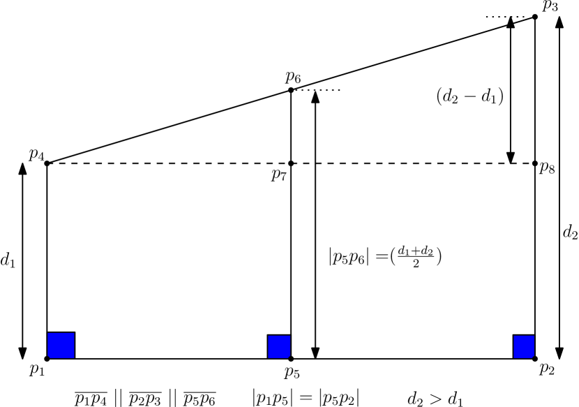
Figure 15: The three parallel edges $\overline{p_{1}p_{4}}$, $\overline{p_{2}p_{3}}$ and $\overline{p_{5}p_{6}}$ in quadrilateral $\Diamond p_{1}p_{2}p_{3}p_{4}$.

Without loss of generality, from now onwards we assume that $\overline{ac}$ lies below $\overline{h_{1}h_{2}}$ and the vertex “$b$” lies to the right of “$v_{1}$” which makes $|ab|\geq\frac{\sqrt{1+W^{2}}}{2}$ (following Observation 7) in $\Diamond abcd$. The perpendicular bisector of the edge $\overline{ab}$ is denoted by $\overline{m_{1}z}$, where $m_{1}$ is the mid-point of $\overline{ab}$. Now, $\overline{m_{1}z}$ intersects $\Diamond abcd$ at the point $z$ (see Figure 15).

Lemma 5.

If one of the adjacent edges of $\overline{ab}$ is of length at least $\frac{\sqrt{1+W^{2}}}{2}$ and the width $W$ of the covering rectangle $\Box efgh$ is at least $\frac{1}{\sqrt{3}}$, then $\alpha\leq 1.6$.

Proof:   In $\Diamond abcd$, the two adjacent edges of $\overline{ab}$ are $\overline{bc}$ and $\overline{ad}$. If $|bc|\geq\frac{\sqrt{1+W^{2}}}{2}$ then we consider $\triangle abc$, and the length of its smallest side $\ell\geq\frac{\sqrt{1+W^{2}}}{2}$. Similarly, if $|ad|\geq\frac{\sqrt{1+W^{2}}}{2}$ then we consider $\triangle abd$ where $|bd|\geq W$. If $W>\frac{1}{\sqrt{3}}$, we have $W>\frac{\sqrt{1+W^{2}}}{2}$ (since $4W^{2}>1+W^{2}$). Hence, $\ell$ (the length of the smallest side of $\triangle abd$) $\geq$ $\frac{\sqrt{1+W^{2}}}{2}$. Thus in $\Diamond abcd$, always there exists a triangle whose smallest side is of length $\ell\geq\frac{\sqrt{1+W^{2}}}{2}$. Thus, $\alpha=\frac{r}{\ell/2}=\sqrt{\frac{1+4W^{2}}{1+W^{2}}}=\sqrt{1+\frac{3}{1+\left(\frac{1}{W^{2}}\right)}}$. This is a monotonically increasing function of $W$, and it attains maximum when $W=1$ to have $\alpha=\sqrt{2.5}<1.6$  $\Box$

Thus Lemma 5 suggests that, we need to consider the case where both the adjacent sides of $\overline{ab}$ are of length strictly less than $\frac{\sqrt{1+W^{2}}}{2}$.

Observation 8.

The perpendicular bisector of $\overline{ab}$ (of the quadrilateral $\Diamond abcd$) cannot intersect the edge $\overline{bc}$ except at its end-point $c$.

Proof:   Refer to Figure 15. In $\Diamond abcd$, the perpendicular bisector ($\overline{m_{1}z}$) of the edge $\overline{ab}$ intersect $\overline{cd}$ at a point $z$. Now, if $b$ is moved towards left on the edge $\overline{eh}$, the point $z$ on $\overline{cd}$ moves towards $c$. At a position $b^{\prime}$ (say) of $b$, the perpendicular bisector $\overline{m^{\prime}_{1}z}$ of $\overline{ab^{\prime}}$ passes through $c$. Then $\triangle ab^{\prime}c$ becomes isosceles with $|b^{\prime}c|=|ac|=1$. If we try to make $\overline{m^{\prime}_{1}z}$ intersect with $\overline{bc}$, we need to move $b$ to the left of $b^{\prime}$. For any such point $b^{\prime\prime}$, we have $|cb^{\prime\prime}|>1$, violating the diameter constraint of $\Diamond abcd$.  $\Box$

Fact 1.

In a quadrilateral $\Diamond p_{1}p_{2}p_{3}p_{4}$, if $\overline{p_{2}p_{3}}$ and $\overline{p_{1}p_{4}}$ are perpendicular to $\overline{p_{1}p_{2}}$, and the segment $\overline{p_{5}p_{6}}$, touching $\overline{p_{1}p_{2}}$ and $\overline{p_{3}p_{4}}$, is the perpendicular bisector of $\overline{p_{1}p_{2}}$ (see Figure 15), then $|p_{5}p_{6}|=\left(\frac{d_{1}+d_{2}}{2}\right)$, where $d_{1}=|p_{1}p_{4}|$ and $d_{2}=|p_{2}p_{3}|$.

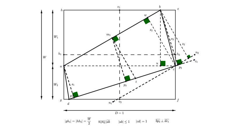
Figure 16: Perpendicular bisector $\overline{m_{1}z}$ of $\overline{ab}$ intersect $\overline{cd}$ at $z$ and $|{m_{1}z}|>\frac{W}{2}$

Lemma 6.

In the quadrilateral $\Diamond abcd$, if the perpendicular bisector $\overline{m_{1}z}$ of $\overline{ab}$ intersects its non-adjacent edge $\overline{cd}$ at a point $z$, then $|m_{1}z|\geq\frac{W}{2}$.

Proof:   Consider the scenario where $\Diamond abcd$ satisfies the following (Figure 16):

• The diagonal $\overline{ac}$ of $\Diamond abcd$ is below $\overline{h_{1}h_{2}}$ so that $|ah|=|ec|=W_{1}\geq W/2$ and $|ag|=|cf|=W_{2}\leq W/2$.

• The point $d$ is chosen on $\overline{fg}$ such that $|cd|=1$. The point $b$ is chosen at any arbitrary position to the right of $v_{1}$ on $\overline{eh}$ such that $|ab|\leq 1$.

We show that in such a scenario, $|{m_{1}z}|\geq W/2$. If we move $d$ to the right (towards $f$) along the edge $\overline{fg}$, keeping $a$, $b$, $c$ fixed, then $|m_{1}z|$ increases.

Let $a$ be the origin of the co-ordinate system, and $|ab|\leq 1$. Thus the vertices of the quadrilateral $\Diamond abcd$ are $b=(\sqrt{|ab|^{2}-W_{1}^{2}},W_{1})$, $c=(1,0)$ and $d=((1-\sqrt{1-W_{2}^{2}}),-W_{2})$. The equation of the lines $\overline{ab}$ and $\overline{cd}$ are given by $y=\frac{W_{1}}{\sqrt{|ab|^{2}-W_{1}^{2}}}x$ and $y=\frac{W_{2}}{\sqrt{1-W_{2}^{2}}}(x-1)$ respectively. Let the point $p_{1}$ be the projection of $a$ on $\overline{cd}$ and the point $w$ be projection of the point $c$ on $\overline{ab}$ (see Figure 16). Let

$$s_{1}=|ap_{1}|=\frac{{\frac{W_{2}}{\sqrt{1-W_{2}^{2}}}}}{\sqrt{1+\left(\frac{W_{2}}{\sqrt{1-W_{2}^{2}}}\right)^{2}}}=W_{2}$$ (5)

$$s_{2}=|cw|=\frac{{\frac{W_{1}}{\sqrt{|ab|^{2}-W_{1}^{2}}}}}{\sqrt{1+\left(\frac{W_{1}}{\sqrt{|ab|^{2}-W_{1}^{2}}}\right)^{2}}}=\frac{W_{1}}{|ab|}\geq W_{1}~{}~{}(\text{since}~{}a\leq 1)$$ (6)

Now, if $u$ is the projection of $b$ on $\overline{ac}$, we have $|bu|=W_{1}$. Thus from Figure 16 we have, $\sin\angle cab=\sin\angle uab=\frac{|bu|}{|ab|}=\frac{W_{1}}{|{ab}|}\geq W_{1}$ (since $|{ab}|\leq 1$) and similarly $\sin\angle acd=\frac{s_{1}}{|ac|}=\frac{W_{2}}{|ac|}=W_{2}$ (since $s_{1}=W_{2}$ from Equation 5, and $|ac|=1$). Since $W_{1}>W_{2}$, we have $\sin\angle cab>\sin\angle acd$ which implies $\angle cab>\angle acd$.

We now draw a line $\overline{n_{1}n_{2}}$ through the point $c$ and parallel to $\overline{ab}$. The perpendicular distance of this line from $b$ is $s_{2}$. The line segment $\overline{dc}$ is extended to $\overline{dc^{\prime}}$ such that it can contain the projection $p_{2}$ of vertex $b$ on the edge $\overline{dc}$ (or on its extension). Now, we consider the two cases:

• If the projection $p_{2}$ of $b$ on $\overline{dc}$ is to the left of $c$, then $|bp_{2}|\geq|bu|=W_{1}$.

• If the projection $p_{2}$ of $b$ on $\overline{dc}$ is to the right of $c$, then since the slope of $\overline{n_{1}n_{2}}$ is greater than that of $\overline{dc^{\prime}}$, we have $|bp_{2}|\geq s_{2}\geq W_{1}$ (see Equation 6).

Let $p_{3}$ be the projection of $m_{1}$ ($m_{1}$ is the mid-point of $\overline{ab}$) on the line $\overline{cd}$. Now, consider the quadrilateral $\Diamond abp_{2}p_{1}$. Using Fact 1, we have $|m_{1}p_{3}|=\frac{s_{1}+s_{2}}{2}\geq\frac{W_{1}+W_{2}}{2}=\frac{W}{2}$ because $s_{1}=W_{2}$ and $s_{2}\geq W_{1}$ (see Equations 5 and 6). Note that, $\overline{m_{1}z}$ is the perpendicular bisector of $\overline{ab}$ which meets $\overline{cd}$ at $z$, and $\overline{m_{1}p_{3}}$ is the perpendicular from $m_{1}$ on $\overline{cd}$. Thus, $|m_{1}z|\geq|m_{1}p_{3}|=\frac{W}{2}$.

Thus, we proved that if $|cd|=1$ then $|m_{1}z|\geq\frac{W}{2}$. Now, for a fixed position of $a$, $b$ and $c$ we reduce $|cd|$ by moving $d$ towards $f$ along the edge $\overline{fg}$. Thus, $|m_{1}z|$ increases further, and hence we have $|m_{1}z|\geq\frac{W}{2}$ at any position of $d$ on $\overline{fg}$.  $\Box$

Theorem 2.

Always there exist a triangle $\triangle$ within the quadrilateral $\Diamond abcd$ so that the length of smallest side of $\triangle$ is at least $\frac{\sqrt{1+5W^{2}}}{4}$.

Proof:   Observation 8 says that the perpendicular bisector $\overline{m_{1}z}$ of $\overline{ab}$ must intersect either $\overline{cd}$ or $\overline{ad}$. We consider these two cases separately.

$\bullet\overline{m_{1}z}$ intersects $\overline{cd}$:

By Lemma 6, $|m_{1}z|>\frac{W}{2}$. Since $|ab|\geq\frac{\sqrt{1+W^{2}}}{2}$ (by the assumption following Observation 7), we can choose the isosceles triangle $\triangle abz$ having equal sides $\overline{az}$ and $\overline{bz}$, and their (common) length satisfies

$$|az|=|bz|\geq\sqrt{\left(\frac{\sqrt{1+W^{2}}}{4}\right)^{2}+\left(\frac{W}{2}\right)^{2}}=\frac{\sqrt{1+5W^{2}}}{4}$$ (7)

As $W\leq 1$, we have $\frac{\sqrt{1+5W^{2}}}{4}<\frac{\sqrt{1+W^{2}}}{2}$. Thus $\ell$, the length of the smallest side of $\triangle abz$ is at least $\frac{\sqrt{1+5W^{2}}}{4}$.

$\bullet\overline{m_{1}z}$ intersects $\overline{ad}$:

Consider the extension of the perpendicular bisector $\overline{m_{1}z}$ (of $\overline{ab}$) that intersects $\overline{fg}$ at $d_{0}$ (see Figure 17). Thus, if the vertex $d$ of $\Diamond abcd$ coincides with $d_{0}$, then $\overline{m_{1}z}$ will touch both $\overline{cd}$ and $\overline{ad}$, and in that case $|m_{1}z|=|m_{1}d_{0}|$. Now, by Lemma 6, we have $|m_{1}d_{0}|=|m_{1}z|>\frac{W}{2}$, and as in Equation 7, we have $|ad_{0}|=\sqrt{|am_{1}|^{2}+|m_{1}d_{0}|^{2}}\geq\frac{\sqrt{1+5W^{2}}}{4}$. In this case, we obtain an isosceles $\triangle abd_{0}$ and the length of its smallest side satisfy $\ell=|ad_{0}|=|bd_{0}|\geq\sqrt{\left(1+5W^{2}\right)}/4$.

However, if $d$ lies to the right of $d_{0}$, say at $d_{1}$ (see dashed lines in Figure 17), we consider $\triangle abd_{1}$, and we have $|ad_{1}|>|ad_{0}|>\frac{\sqrt{1+5W^{2}}}{4}$ and $|bd_{1}|>~{}W>~{}\frac{\sqrt{1+W^{2}}}{2}$ (as $W>\frac{2}{\sqrt{5}}$ implies $W>\frac{1}{\sqrt{3}}$, i.e. $4W^{2}>1+W^{2}$). Now $\frac{\sqrt{1+5W^{2}}}{4}<\frac{\sqrt{1+W^{2}}}{2}$ for $W<\sqrt{3}$ which is obvious because $W\leq D=1<\sqrt{3}$. Therefore, in this case also the length of the smallest side ($\ell$) of a triangle satisfy $\ell\geq\frac{\sqrt{1+5W^{2}}}{4}$.

 $\Box$

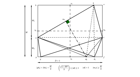
Figure 17: The perpendicular bisector of $\overline{ab}$ can intersect the edge $\overline{ad}$ of $\Diamond~{}abcd$ if $d$ lies at the right of $d_{0}$

Thus we have the approximation factor

$$\alpha=\frac{r}{\ell/2}=\frac{\frac{\sqrt{1+4W^{2}}}{4}}{\frac{\sqrt{1+5W^{2}}}{8}}=2\sqrt{\frac{1+4W^{2}}{1+5W^{2}}}=2\sqrt{1-\frac{1}{\left(5+\frac{1}{W^{2}}\right)}},$$ (8)

which is a decreasing function in $W$.

Lemma 7.

The approximation factor $\alpha$ for two-center problem of a quadrilateral $\Diamond abcd$ is given by $\alpha<1.84$.

Proof:   The increasing and decreasing nature of the value of $\alpha$ with respect to $W$ in Equations (4) and (8), respectively suggest a threshold value of $W$ based on which we decide which triangle is to be selected inside the quadrilateral $\Diamond abcd$. Equating the expressions of $\alpha$ in Equations (4) and (8), we have

$$\frac{\sqrt{(1+W^{2})(4-W^{2})}}{2}=2\sqrt{\frac{4W^{2}+1}{5W^{2}+1}}\\ \Rightarrow(5W^{2}-4)(W^{2}-3)(4W^{2}+1)=0$$ (9)

The only feasible solution of the above equation is $W={2}/{\sqrt{5}}=0.8944$. The approximation factor $\alpha$ at $W=\frac{2}{\sqrt{5}}$ using Equation 8 is given by $\alpha=1.833<1.84$. Thus the result in the stated theorem is justified as follows:

• $W<\frac{2}{\sqrt{5}}$ : Choose the isosceles triangle $\triangle acv_{3}$ with its smallest side $\ell=|{av_{3}}|$ as in Figure 13.

• $W\geq\frac{2}{\sqrt{5}}$ : based on the intersection between $\overline{cd}$ and the perpendicular bisector $\overline{m_{1}z}$ of $\overline{ab}$, the following two sub-cases occur:

  1. $\overline{m_{1}z}$ intersect $\overline{cd}$ at $z$: Choose the isosceles triangle $\triangle abz$ with its smallest side $\ell\geq\frac{\sqrt{1+5W^{2}}}{4}$.

  2. $\overline{m_{1}z}$ intersect $\overline{ad}$ : Choose the triangle $\triangle abd$ with its smallest side $\ell\geq\frac{\sqrt{1+5W^{2}}}{4}$.

 $\Box$

Theorem 3.

The approximation factor $\alpha$ for two-center problem of a given convex polygon $P$ is given by $\alpha<1.84$.

Proof:   Observation 4 says that the approximation factor $\alpha$ for two-center problem of a given convex polygon $P$ is less than (or equal to) that of its minimal subpolygon $\Pi=\Diamond abcd$, where both $P$ and $\Pi$ are exactly covered by the rectangle $\cal R$. Now, the result follows from Lemma 7.  $\Box$

3.2.3 Special Case: $W=D=1$

We now show one special case when the covering rectangle R is a square i.e., $W=D=1$ (see Figure 18). This will give us an idea that the upper bound of the approximation factor of our algorithm cannot be smaller than $1.527$. Any quadrilateral inscribed within this “square $efgh$” must be of a diamond shape (i.e. the $x-$coordinate of two points $b$ and $d$ must be equal). There are two extreme situations: one with $|ab^{\prime}|=1$, where the corresponding quadrilateral is $\Diamond ab^{\prime}cd^{\prime}$ and the other one is a square $\Diamond abcd$ (Figure 18) respectively.

(i) For quadrilateral $\Diamond abcd$:

Refer to Figure 18. Since $|ab^{\prime}|=|ad^{\prime}|=|b^{\prime}d^{\prime}|=|ac|=1$, we have $\angle cab^{\prime}=30^{o}$. Now $\angle cab=45^{o}$ because $\Diamond abcd$ is a square. The points $t_{1}$ and $t_{2}$ are the points of intersection of $\overline{ab^{\prime}}$ with $\overline{bc}$, and $\overline{ad^{\prime}}$ with $\overline{cd}$ respectively Therefore, $\frac{|{co_{2}}|}{|{o_{2}t_{1}}|}=1$ and $\frac{|{ao_{2}}|}{|{o_{2}t_{1}}|}=\sqrt{3}$. Now $|{ao_{2}}|+|{co_{2}}|=1$ gives $|{o_{2}t_{1}}|=\frac{1}{\sqrt{3}+1}$. So, length of each side of the equilateral $\triangle at_{1}t_{2}$ is given by $|t_{1}t_{2}|=2|o_{2}t_{1}|=\frac{2}{\sqrt{3}+1}$. Therefore, the equilateral triangle $\triangle at_{1}t_{2}$ inscribed within quadrilateral $\Diamond abcd$ have the side $|{at_{1}}|=\frac{2}{\sqrt{3}+1}=0.732$, whereas the isosceles triangle $\triangle abc$ has the smallest side $|{ab}|=\frac{1}{\sqrt{2}}=0.7071$. Thus the smallest side $\ell$ of the triangle $\triangle at_{1}t_{2}$ is the largest inside the $\Diamond abcd$ and we consider $\triangle at_{1}t_{2}$ with $\ell=\frac{2}{\sqrt{3}+1}$. Hence the approximation factor $\alpha=\frac{r}{\ell/2}={\frac{(\sqrt{5})}{4}}/{\frac{1}{(\sqrt{3}+1)}}=1.527$.

Figure 18: The covering rectangles of the quadrilateral $\Diamond abcd$ is “square $efgh$”

(ii) For quadrilateral $\Diamond ab^{\prime}cd^{\prime}$:

The largest equilateral triangle inscribed within the quadrilateral $\Diamond ab^{\prime}cd^{\prime}$ is $\triangle ab^{\prime}d^{\prime}$ (see Figure 18) whose sides are all $1$. Thus $\ell=1$, and the approximation factor $\alpha=\frac{r}{\ell/2}$ = $\left({\frac{\sqrt{5}}{4}}\right)/\left(\frac{1}{2}\right)=1.118$.

The lower bound of $\ell$ for any quadrilaterals $\Diamond abcd$ inscribed within the square $efgh$, where the range of $b$ on the edge $\overline{he}$ is given by $x(b^{\prime\prime})\leq x(b)\leq x(b^{\prime})$, will be the intermediate of the lower bounds for quadrilaterals $\Diamond abcd$ and $\Diamond ab^{\prime}cd^{\prime}$. Hence if the covering rectangle $\Box efgh$ is a square, the approximation factor $\alpha$ will satisfy $1.118\leq\alpha\leq 1.527$. This shows that our technique can not produce a solution with approximation factor less than $1.527$, because we need to consider all possible convex polygons for this problem.

4 Conclusion and future work

To the best of our knowledge, this is the first work on approximation for two-center problem of a given convex polygon both in streaming and non-streaming setup. In the streaming setup, we have designed a $2$-factor approximation algorithm using $O(1)$ space for this problem; whereas in the non-streaming setup, we have proposed a linear time approximation algorithm with approximation factor $1.84$. The “longest line segment inside a quadrilateral” and “the triangle which makes its smallest side larger” have been considered to determine the lower bound for the radius of the two-center problem of a given convex polygon.

The main bottleneck of adopting the 1.84 factor approximation algorithm in the streaming model is the unavailability of an algorithm for computing the diameter of a convex polygon in streaming model. Thus, getting such an algorithm will be an interesting problem to study.

Surely, improving or establishing non-trivial lower bounds for the approximation results of this problem will be the main open problems.

References

- [1] Agarwal, P.K., Sharathkumar, R.: Streaming algorithms for extent problems in high dimensions. Algorithmica 72(1), 83–98 (2015)
- [2] Agarwal, P.K., Sharir, M., Welzl, E.: The discrete 2-center problem. In: Discrete and Computational Geometry. vol. 20(3), pp. 238–255. Springer US (1998)
- [3] Bespamyatnikh, S., Kirkpatrick, D.G.: Rectilinear 2-center problems. In: Proceedings of the 11th Canadian Conference on Computational Geometry (CCCG) (1999)
- [4] Chan, T.M.: More planar two-center algorithms. In: Computational Geometry: Theory and Applications. vol. 13(3), pp. 189–198 (1999)
- [5] Chan, T.M., Pathak, V.: Streaming and dynamic algorithms for minimum enclosing balls in high dimensions. Computational Geometry: Theory and Applications 47(2), 240–247 (2014)
- [6] Das, G.K., Das, S., Nandy, S.C., Sinha, B.P.: Efficient algorithm for placing a given number of base stations to cover a convex region. Journal of Parallel Distributed Computing 66(11), 1353–1358 (2006)
- [7] Eppstein, D.: Faster construction of planar two-centers. In: 8th ACM-SIAM Symposium On Discrete Algorithms (SODA). pp. 131–138 (1997)
- [8] Guha, S.: Tight results for clustering and summarizing data streams. In: 12th International Conference on Database Theory. pp. 268–275. ACM International Conference Proceeding Series (2009)
- [9] Hershberger, J.: A fast algorithm for the two-Center decision Problem. Information Processing Letters (Elsevier) 47(1), 23–29 (1993)
- [10] Jaromczyk, J.W., Kowaluk, M.: An Efficient Algorithm for the Euclidean Two-Center Problem. In: Mehlhorn, K. (ed.) Symposium on Computational Geometry. pp. 303–311. ACM (1994)
- [11] Katz, M.J., Kedem, K., Segal, M.: Discrete rectilinear 2-center problems. Comput. Geom. 15(4), 203–214 (2000)
- [12] Kim, S.S., Ahn, H.K.: An improved data stream algorithm for clustering. Computational Geometry: Theory and Applications 48(9), 635–645 (2015)
- [13] Kim, S.K., Shin, C.S.: Efficient algorithms for two-center problems for a convex polygon. In: 6th Annual International Conference, COCOON 2000 Sydney, Australia. pp. 299–309. Springer Berlin Heidelberg (2000)
- [14] Marchetti-Spaccamela, A.: The p center problem in the plane is NP complete. In: In Proc. 19th Allerton Conf. Commun. Control Comput. pp. 31–40 (1981)
- [15] McCutchen, R.M., Khuller, S.: Streaming algorithms for k-Center clustering with outliers and with anonymity. In: Approximation, Randomization and Combinatoral Optimization. Algorithms and Techniques. vol. 5171, pp. 165–178 (2008)
- [16] Plesnik, J.: A heuristic for the p-center problem in graphs. Discrete Applied Mathematics 17, 263–268 (1987)
- [17] Shamos, M.I.: Computational Geometry. Ph.D. thesis, Yale University (1978)
- [18] Sharir, M.: A near-linear algorithm for the planar 2-center problem. Discrete & Computational Geometry 18(2), 125–134 (1997)
- [19] Vigan, I.: Packing and covering a polygon with geodesic disks. In: CoRR abs/1311.6033 (2013)