Charge Transfer in Ultracold Rydberg-Ground State Atomic Collisions

Abstract

In excited molecules, the interaction between the covalent Rydberg and ion-pair channels forms a unique class of excited Rydberg states, in which the infinite manifold of vibrational levels are the equivalent of atomic Rydberg states with a heavy electron mass. Production of the ion pair states usually requires excitation through one or several interacting Rydberg states; these interacting channels are pathways for loss of flux, diminishing the rate of ion pair production. Here, we develop an analytical, asymptotic charge transfer model for the interaction between ultracold Rydberg molecular states, and employ this method to demonstrate the utility of off-resonant field control over the ion pair formation, with near unity efficiency.

I Introduction

Ultracold atomic systems allow for precise control via laser and static fields and are employed for simulating strongly-correlated many-body condensed matter and optical systems, for performing chemistry in the quantum regime, and for executing quantum computing protocols  Bloch et al. (2008); Regal et al. (2003); Carr et al. (2009). Excitations in ultracold atomic traps have ushered in the Rydberg blockade regime Lukin et al. (2001); Saffman et al. (2010) (with promise for quantum information processing and quantum bit operations), ultracold plasmas Castro et al. (2009) (with application in recombination, ion crystal order and heating), and ultra long range Rydberg molecules Greene et al. (2000); Bendkowsky et al. (2009) (for studies of few-body molecular systems, symmetry breaking Li et al. (2011); Booth et al. (2015) and coherent control Rittenhouse and Sadeghpour (2010)).

Another class of molecular states, the ion pair states, form channels when the covalent Rydberg channels couple to the long-range ion-pair potential. These atomic cation-anion pair states share several properties with ionic molecules; an infinite spectrum of vibrational levels which follow a Rydberg progression with a heavy electron mass, and large permanent electric dipole moments. They are also long-range states and have typically negligible Franck-Condon (FC) overlap with the usual short-range molecular levels. These heavy Rydberg states (HRS) have been experimentally observed in several molecular species, relying on excitation from bound molecular levels  Vieitez et al. (2008, 2009); Mollet and Merkt (2010); Ekey and McCormack (2011).

The prevailing issue with indirect excitation of bound molecules, such as in H₂ and Cl₂ Vieitez et al. (2008, 2009); Mollet and Merkt (2010); Ekey and McCormack (2011), is that it is not a priori possible to identify a set of long-lived intermediate heavy Rydberg states to which ion the pair states couple. In a recent work Kirrander et al. (2013), it was proposed to directly pump long-lived HRS from ultracold Feshbach molecular resonances, just below the avoided crossings between the covalent potential energy curves and the ion-pair channel. The predominant excitation to HRS occurs near the avoided crossings, because the non-adiabatic mixing allows for favorable electronic transitions to the HRS. When the nuclear HRS wave function peaks at the classical turning point, the internuclear FC overlap increases.

In this work, we develop an analytical, but asymptotic model for one-electron transfer, merging single-center potentials for the Rb atom, and demonstrate efficient field control over the rate of ion pair formation. Adiabatic potential energy curves are calculated along with the radial non-adiabatic coupling and dipole transition matrix elements. We compare our adiabatic potential energies with the Born-Oppenheimer (BO) potential energy curves from Ref. Park et al. (2001). We find that with modest off-resonant external fields, we can alter the avoided crossing beween the covalent HRS and ion pair channels, and modify the behavior of the nuclear wavefunction at the classical turning points; hence, control the FC overlaps and rate of ion pair formation.

This excitation occurs at larger internuclear separations, where the overlap and transition dipole moments between the ground and ion pair states are significant. The method proposed in Kirrander et al. (2013) requires adiabatic rapid passage or multiphoton transitions to enhance this excitation, while in the present work, only off-resonant fields must be employed to increase the efficiency of ion pair production.

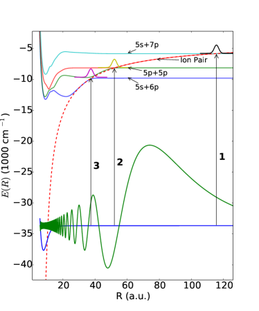
Figure 1: Scheme from Kirrander et al. (2013) relied on excitation to the Rb(5s)+Rb(6p)/Rb⁺+Rb^- (ion pair) or Rb(5p)+Rb(5p)/ion pair crossings (excitation 2 and 3). Here, we focus on the Rb(5s)+Rb(7p)/ion pair crossing (excitation 1). Subsequent to excitation, both schemes from Kirrander et al. (2013) require multiphoton excitation or chirped pulse rapid adiabatic passagee. Excitation 1, directly to the Rb(5s)+Rb(7p)/ion pair crossing, can more easily be controlled with dc electric fields. Additionally, the Franck-Condon factors for this excitation are favorable, as demonstrated by the $\nu=124$ Feshbach molecule vibrational wavefunction. The dashed curve is the ion pair potential.

II Methodology and Results

The present charge transfer model relies on one active electron participating in the process of ion pair excitation. For the charge transfer to occur, the Rb valence electron is ionized from one center, separated from the other neutral center by a distance $R$. The ionization process is calculated in the one-electron effective potential model of Ref. Marinescu et al. (1994). The interaction of the electron with the neutral Rb atom is modeled by the short-range scattering of the low-energy electron from the ground-state Rb atom. This is done with a symmetric inverse hyperbolic cosine (Eckart) potential.

The two-center Hamiltonian matrix elements are constructed by expanding in a basis of atomic Rb Rydberg orbitals and the single bound orbital in the Eckart potential. The resulting generalized eigenvalue equation is solved for the adiabatic potential energy curves, radial coupling and electronic dipole matrix elements. Our control scheme hinges on modifying the avoided crossing gap between the 5s+7p and ion pair state by applying an off-resonant field, thereby tuning the Landau-Zener crossing probabilities between the ion pair and covalent states.

The two-center potential for the Rb₂ Rydberg-excited molecule is the sum of two single-center potentials,

$$V_{\text{model}}(r_{a},r_{b}|R)=V_{1}(r_{a}|R)+V_{2}(r_{b}|R)$$ (1)

where $V_{1}$ represents the potential felt by the valence electron due to the Rb core, and the pseudopotential $V_{2}$ that of the binding to the neutral rubidium atom; $r_{a}$ and $r_{b}$ represent the distances between the electron and the cation/neutral atom, respectively.

We require that the potential in Eq. 1 correctly reproduce the asymptotic dissociation energies for all the relevant Rydberg and ion-pair states et. al. . We further enforce that the known energy-independent $e^{-}\text{-Rb}$ scattering length and the Rb electron affinity are reproduced, i.e. $a_{sc}=-16.1$ a.u. Bahrim et al. (2001) and EA=-0.01786 a.u. et. al. .

The valence-electron potential, $V_{1}$ Marinescu et al. (1994) correctly reproduces the observed atomic energies  et. al. ,

$$V_{1}(r_{a})=-\frac{Z_{l}(r_{a})}{r_{a}}-\frac{\alpha_{c}}{2r_{a}^{4}}(1-e^{-(r_{a}/r_{c})^{6}})$$ (2)

where

$$Z_{l}(r_{a})=1+(z-1)e^{-\alpha_{1}r_{a}}-r(a_{3}+a_{4}r_{a})e^{-a_{2}r_{a}}$$

with $z$ being the nuclear charge. The terms of the potential account for screening of the nuclear charge due to core electrons and effect of core polarizability.

For the neutral rubidium electron affinity, we use the radial Eckart potential Eckart (1930).

$$V_{2}(r_{b})=V_{0}\cosh^{-2}{(\frac{r_{b}}{r_{0}})}$$ (3)

where $V_{0}$ and $r_{0}$ are parameters related in a set of coupled equations to the electron affinity and $e^{-}\text{-Rb}$ scattering length; see appendix A.

The Hamiltonian matrix is constructed from a suitable basis for each center and may be conveniently represented in prolate spheroidal coordinates

$$r=\frac{R}{2}(\xi+\kappa\eta),\ \cos{\theta}=\frac{1+\kappa\xi\eta}{\xi+\kappa\eta}$$

where $\kappa=+1(-1)$ represents the radial coordinate of the left(right) centers, $\xi\in[1,\infty),\ \eta\in[-1,1]$.

We solve the generalized eigenvalue problem:

$$\mathbf{H}\vec{\Psi}=E(R)\mathbf{S}\vec{\Psi}$$ (4)

where $\mathbf{H}$ and $\mathbf{S}$ are the Hamiltonian and overlap matrices in the truncated basis:

$$\mathbf{H}_{jj^{\prime}}=\bra{\phi_{j}^{(a)}}H_{0}^{(a)}+V_{2}\ket{\phi_{j}^{(a)}}$$ (4a)

$$\mathbf{H}_{kk^{\prime}}=\bra{\phi_{k}^{(b)}}H_{0}^{(b)}+V_{1}\ket{\phi_{k}^{(b)}}$$ (4b)

$$\mathbf{H}_{jk}=\bra{\phi_{j}^{(a)}}H_{0}^{(b)}+V_{1}\ket{\phi_{k}^{(b)}}=\bra{\phi_{k}^{(b)}}H_{0}^{(a)}+V_{2}\ket{\phi_{j}^{(a)}}$$ (4c)

$$\mathbf{S}_{jj^{\prime}}=\braket{\phi_{j}^{(a)}}{\phi_{j}^{\prime(a)}}=\delta_{jj^{\prime}}$$ (4d)

$$\mathbf{S}_{kk^{\prime}}=\braket{\phi_{k}^{(b)}}{\phi_{k}^{\prime(b)}}=\delta_{kk^{\prime}}$$ (4e)

$$\mathbf{S}_{jk}=\braket{\phi_{j}^{(a)}}{\phi_{k}^{(b)}}$$ (4f)

The full wave function is comprised of $\{\phi_{j}^{(a)}(\frac{R}{2}(\xi+\eta)\}$ centered on $V_{1}$, and $\{\phi_{k}^{(b)}(\frac{R}{2}(\xi-\eta)\}$ centered on $V_{2}$, i. e. $\Psi_{i}=\sum_{j}^{n_{a}}c_{ij}\phi_{j}^{(a)}+\sum_{k}^{n_{b}}c_{ik}\phi_{k}^{(b)}$. The truncated basis set contains atomic orbitals, $\{\phi_{j}^{(a)}\}=\{(5\text{-}9)s,(5\text{-}11)p,(4\text{-}6)d\}$, and the short-range wave function for scattering the of electrons from $V_{2}$, $\{\phi_{k}^{(b)}\}=\{\cosh^{-2\lambda}\frac{r_{b}}{r_{0}}\sqrt{z}\ {}_{2}F_{1}(0,-2\lambda,\frac{3}{2},z)\}$, with $z=-\sinh^{2}{(\frac{r_{b}}{r_{0}})},\ \mbox{and}\ \lambda=0.0321816$; see Appendix A. ${}_{2}F_{1}(a,b;c;z)$ is the hypergeometric function  Bateman Manuscript Project et al. (1954).

One major feature of this asymptotic approach is that the permanent and transition dipole, and non-adiabatic radial coupling matrix elements can now be calculated from the eigenstates of Eq. 4. Full details are available in Appendix A. The adiabatic potential energy curves, $E(R)$, are shown in Fig. 2. By construction, these adiabatic potentials correlate to the asymptotic dissociation energies for the Rydberg and ion pair states and have avoided crossings between covalent and ion pair channels. The Rb₂ BO potential energies in the region of Rb(5s)+Rb(6p) dissociation energy are superposed on the adiabatic potentials for comparison. The non-adiabatic coupling matrix element between the ion pair channel with the molecular Rydberg curve dissociating to Rb(5s)+Rb(7s) is shown in the inset of Fig. 2.

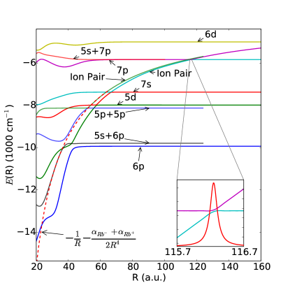
Figure 2: Nuclear potential energy curves, overlaid with calculations from other publications. Calculated curves are well-behaved in the large R limit. Inset shows avoided crossing at $R_{c}=116.2$, along with non-adiabatic coupling matrix element between Rb(5s)+Rb(7p)/ion pair channels. Rb(5s)+Rb(6p), Rb(5p)+Rb(5p), and ion pair curves taken from Rb(5s)+Rb(6p), Rb(5p)+Rb(5p), Rb(5s)+Rb(7p), and ion pair curves taken from  Park et al. (2001)  Bellos et al. (2013). Ion pair curve is fitted to $-\frac{1}{R}-\frac{\alpha_{\text{Rb}_{-}}+\alpha_{\text{Rb}_{+}}}{2R^{4}}$, where $\alpha_{\text{Rb}_{-}}=526.0$ a.u  Fabrikant , $\alpha_{\text{Rb}_{+}}=9.11$ a.u  Mitroy et al. are the polarizabilities of the anion and cation respectively.

III Field Control Covalent/Ion Pair Channels

The avoided crossing in the interaction of ion pair channel (Rb⁺+Rb^-) and Rydberg channel (Rb(5s)+Rb(7p)) is nearly diabatic, i. e. the covalently populated vibrational states will predominantly dissociate to neutral atoms with little possibility of forming HRS and ion pair states. This is reflected in the narrowness of the avoided crossing and the strength of the radial non-adiabatic matrix element. The two channels have non-zero dipole transition moments, so in an external field, they will mix and modify the transition probability for populating ion pair states.

Near the avoided crossing, the electronic wave function becomes hybridized in the field, as in the first order of perturbation theory, $\ket{\psi}=\ket{\psi_{0}}+\sum_{k\neq 0}\frac{\bra{\psi_{k}}-\mathbf{F}\cdot\mathbf{z}\ket{\psi_{0}}}{E_{0}-E_{k}}\ket{\psi_{k}}$, where $\ket{\psi_{k}}$ are the dipole-allowed states which couple to the initial state, $\ket{\psi_{0}}$. This hybridization is demonstrated in Fig. 3 for the two channels of interest. When the field is off, the wave function amplitude in the covalent Rydberg channel peaks near the avoided crossing. With the field on, the two amplitudes become comparable.

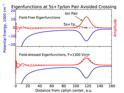
Figure 3: Hybridization of the wavefunctions at the avoided crossing by the field. The upper panel show the cross section of the field-free electronic wavefunction along the internuclear axis—states associated with the ion pair and Rb(5s)+Rb(7p) channels have very little overlap. The lower panel is field-dressed ($\mathbf{F}=1300$ V/cm, showing significant overlap of the wavefunctions associated with the two channels. The blue line is the pseudopotential along the internuclear axis for $R=116.2$ a.u.

The probability that ion-pair states survive the single-pass traversal through the avoided crossing region in Fig.  2 is given approximately by the Landau-Zener-Stückelberg formula:

$$P_{\text{ad}}=1-\exp{[-2\pi\frac{a^{2}}{|v\frac{\partial(E_{2}-E_{1})}{\partial R}|}]}$$ (5)

where $v=\sqrt{\frac{2(E-V(R_{c}))}{m}}$ is the velocity of the wavepacket at crossing, $R=R_{c}$, $a$ is the off-diagonal element coupling the two states at $R_{c}$ (half the crossing size in the fully diagonalized picture), and $\frac{\partial(E_{2}(R)-E_{1}(R))}{\partial R}|_{R=R_{c}}$ is the relative slope of the intersecting curves at $R=R_{c}$.

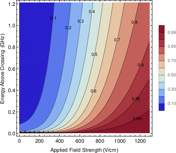
Figure 4: How the ion-pair survival probability may be controlled with modest off-resonant electric fields: Perturbation theory becomes unreliable for F $>1700$ V/cm, and classical ionization occurs for F $>5$ MV/cm. The vertical width of contour regions gives a measure of the survival probability above a desired threshold for a laser-pulse-excited vibrational wavepacket. For example, at $\mathbf{F}\simeq 1000$V/cm., more than 2 $\sigma_{\text{std}}$ will survive if the laser linewidth can be constrained to $\sim 150$ MHz.

Fig.  4 illustrates how the ion=pair probability can be controlled with modest electric fields. Each curve represents a contour of cross-sectional survival probability for a vibrational wavepacket excited to a certain energy above the crossing threshold at a given field strength. For example, at field strengths of $1000$V/cm., more than 2 $\sigma_{\text{std}}=95.45\%$ will survive if the laser linewidth can be constrained to $\sim 150$ MHz.

As the loss probability of a given vibrational level goes at weak field strength as $e^{-\mathbf{F}^{4}}$, even relatively weak fields have a profound effect on ion pair state survival.

IV Conclusion

We have shown that application of weak off-resonant electric fields provide a simple yet potent means of drastically increasing the survivability of the ion pair states in Rb dimers. To this end, we have introduced a simple and intuitive analytical pseudopotential which reproduces the correct asymptotic behavior of the dimer. This model provides an easy and computationally straightforward way for us to calculate dipole and non-adiabatic coupling matrix elements for excited states of alkali dimers.

This work was supported by the National Science Foundation through a grant for the Institute for Theoretical Atomic, Molecular, and Optical Physics at Harvard University and Smithsonian Astrophysical Observatory; S. Markson was additionally supported through a graduate research fellowship through the National Science Foundation.

Appendix A The Eckart potential

A.1 Bound states

Taking the Schrödinger equation with $V(r)$ from  3, we make the substitutions Gol’dman et al. (2006)

$$\psi=(\cosh\frac{r}{r_{0}})^{-2\lambda}u,\ \text{where}\ \lambda=\frac{1}{4}(\sqrt{\frac{8\mu V_{0}{r_{0}}^{2}}{\hbar^{2}}+1}-1)$$

The Schrödinger equation then becomes

$$\frac{d^{2}u}{dr^{2}}-\frac{4\lambda}{r_{0}}\tanh{(\frac{r}{r_{0}})}\frac{du}{dr}+\frac{4}{{r_{0}}^{2}}(\lambda^{2}-\chi^{2})u=0$$ (6)

with

$$\chi=\sqrt{-\frac{\mu E{r_{0}}^{2}}{2\hbar^{2}}}$$

Letting $z=-\sinh^{2}(\frac{r}{r_{0}})$ leads us to the hypergeometric equation

$$z(1-z)\frac{d^{2}u}{dz^{2}}+(\gamma-(\alpha+\beta+1)z)\frac{du}{dz}-\alpha\beta u=0$$ (7)

where $\gamma=\frac{1}{2},\ \alpha=\chi-\lambda,\ \beta=-\chi-\lambda$.

In spherical coordinates, only odd hypergeometric solutions are valid:

$$u=\sqrt{z}\ F(-\lambda+\chi+\frac{1}{2},-\lambda-\chi+\frac{1}{2};\frac{3}{2};z)$$ (8)

By enforcing asymptotic boundary conditions for the bound states ($u\rightarrow 0$ as $r\rightarrow\infty$), we have that

$$\lambda-\chi=n+\frac{1}{2},\ n=0,1,2,\cdots$$

giving the set of bound states

$$\psi_{n}=(\cosh\frac{r}{r_{0}})^{-2\lambda}u_{n}$$ (9)

where

$$u_{n}=N\sinh(\frac{r}{r_{0}})F(-n,-2\lambda+n+1;\frac{3}{2};-\sinh^{2}(\frac{r}{r_{0}}))$$

(N being a normalizing constant), with corresponding energies

$$E_{n}=-\frac{2\hbar^{2}}{\mu{r_{0}}^{2}}(\frac{1}{4}\sqrt{\frac{8\mu V_{0}{r_{0}}^{2}}{\hbar^{2}}+1}-n-\frac{3}{4})^{2}$$ (10)

A.2 Scattering States

With $E=\frac{\hbar^{2}k^{2}}{2\mu}$, $\chi^{2}=-\frac{\mu E{r_{0}}^{2}}{2\hbar^{2}}\rightarrow ikr_{0}=2\chi$ Gol’dman et al. (2006), and

$$u(r)=N\sinh{(\frac{r}{r_{0}})}F(-\lambda+\frac{ikr_{0}}{2}+\frac{1}{2},\\ -\lambda-\frac{ikr_{0}}{2}+\frac{1}{2},\frac{3}{2},-\sinh^{2}\frac{r}{r_{0}})$$

fulfilling the boundary conditions

$$\lim_{r\rightarrow 0}u(r)=0,\ \lim_{r\rightarrow\infty}u(r)\simeq\sin(kr+\delta_{0})$$

where $\delta_{0}$ is the usual phase shift.

We note that $F(\alpha,\beta;\gamma;0)=1,\ \forall\alpha,\beta,\gamma$, and that

$$\lim_{r\to\infty}{\sinh^{2}}(\frac{r}{r_{0}})\approx{\frac{1}{2}}e^{\frac{2r}{r_{0}}}$$

Using the asymptotic behavior of the Gaussian hypergeometric functions (see  Bateman Manuscript Project et al. (1954), p. 108, equation 2).

$$u(r)=Ae^{ikr}+Be^{-ikr}$$

where

$$A=2^{-ikr_{0}}\frac{\Gamma(ikr_{0})}{\Gamma(\frac{1-2\lambda+ikr_{0}}{2})\Gamma(1+\frac{2\lambda+ikr_{0}}{2})},\ B=A^{\dagger}$$

where we neglect a real factor common to $A$ and $B$ which will not affect the scattering phase shift. The phase shift itself has the form:

$$\delta_{0}=\frac{1}{2i}\ln(-\frac{A}{A^{\dagger}})$$ (11)

In the limit $ka\ll 1$, the Gamma functions may be expanded in a Taylor series,

$$\Gamma(ikr_{0})\simeq\frac{1}{ikr_{0}}\Gamma(1+ikr_{0})\simeq\frac{1+ikr_{0}\psi(1)}{ikr_{0}}\Gamma(1)$$

$$\Gamma(\frac{1-2\lambda}{2}+\frac{ikr_{0}}{2})\simeq\Gamma(\frac{1-2\lambda}{2})(1+\frac{ikr_{0}}{2}\psi^{(0)}(\frac{1-r_{0}}{2}))$$

$$\Gamma(1+\frac{2\lambda}{2}+\frac{ikr_{0}}{2})\simeq\Gamma(1+\lambda)(1+\frac{ikr_{0}}{2}\psi^{(0)}(1+\lambda))$$

where $\psi^{(0)}$ is the $m^{th}$-order polygamma function, i.e. $\psi^{(0)}(x)=\frac{d}{dx}\ln\Gamma(x)$. The final expression for $\delta_{0}$ now becomes:

$$\delta_{0}=kr_{0}[-\ln(2)+\psi^{(0)}(1)-\frac{1}{2}\psi^{(0)}(\frac{1-2\lambda}{2})-\frac{1}{2}\psi^{(0)}(1+\lambda)]$$ (12)

which is related to the s-wave scattering length by the usual formula,

$$\lim_{k\rightarrow 0}k\cot{\delta_{0}}=-\frac{1}{a_{sc}}$$

The parameters for the pseudopotential $V_{2}(r)$ ( 3) are hence found by solving the system of equations:

$$a_{s}=r_{0}(-ln(2)+\psi(1)-\frac{1}{2}\psi(\frac{1-2\lambda}{2})-\frac{1}{2}\psi(1+\lambda))$$ (13)

and

$$EA=-\frac{\hbar^{2}}{2\mu{r_{0}}^{2}}(\frac{1}{2}\sqrt{\frac{8\mu V_{0}{r_{0}}^{2}}{\hbar^{2}}+1}-\frac{3}{2})^{2}$$ (14)

There are multiple solutions to Eqs. (A8 - A9). However, since it is known that Rb^- has only one bound state, we impose the additional restriction:

$$N_{\text{bound}}=\lfloor\frac{1}{4}\sqrt{\frac{8\mu V_{0}r_{0}^{2}}{\hbar^{2}}+1}+\frac{1}{4}\rfloor=1$$

The solutions to Eqs. (A8-A9) yield $r_{0}=9.004786$ a.u. and $V_{0}=0.061675$ a.u.

Appendix B Dipole and Non-Adiabatic Coupling Matrix Elements

Dipole elements take the usual form:

$$\vec{d}_{mn}=\bra{\psi_{m}}r\cos{\theta}\ket{\psi_{n}}$$

Non-adiabatic coupling matrix elements are computed via the finite difference formula:

$$A_{mn}=\frac{1}{2\Delta R}(\gamma_{mn}(R|R+\Delta R)-\gamma_{mn}(R|R-\Delta R))$$

where

$$\gamma_{mn}(R|R\pm\Delta R)=\bra{\psi_{m}(r|R)}\ket{\psi_{n}(r|R\pm\Delta R)}$$

References

- Bloch et al. (2008) I. Bloch, J. Dalibard, and W. Zwerger, 80, 885 (2008).
- Regal et al. (2003) C. A. Regal, C. Ticknor, J. L. Bohn, and D. S. Jin, 424, 47 (2003).
- Carr et al. (2009) L. D. Carr, D. DeMille, R. V. Krems, and J. Ye, 11, 055049 (2009).
- Lukin et al. (2001) M. D. Lukin, M. Fleischhauer, R. Cote, L. M. Duan, D. Jaksch, J. I. Cirac, and P. Zoller, 87, 037901 (2001).
- Saffman et al. (2010) M. Saffman, T. G. Walker, and K. Mølmer, 82, 2313 (2010).
- Castro et al. (2009) J. Castro, P. McQuillen, H. Gao, and T. C. Killian, 194, 012065 (2009).
- Greene et al. (2000) C. H. Greene, A. S. Dickinson, and H. R. Sadeghpour, 85, 2458 (2000).
- Bendkowsky et al. (2009) V. Bendkowsky, B. Butscher, J. Nipper, J. P. Shaffer, R. Löw, and T. Pfau, 458, 1005 (2009).
- Li et al. (2011) W. Li, T. Pohl, J. M. Rost, et al., 334, 1110 (2011).
- Booth et al. (2015) D. Booth, S. T. Rittenhouse, J. Yang, H. R. Sadeghpour, and J. P. Shaffer, 348, 99 (2015).
- Rittenhouse and Sadeghpour (2010) S. T. Rittenhouse and H. R. Sadeghpour, 104, 243002 (2010).
- Vieitez et al. (2008) M. O. Vieitez, T. I. Ivanov, E. Reinhold, C. A. de Lange, and W. Ubachs, 101, 163001 (2008).
- Vieitez et al. (2009) M. O. Vieitez, T. I. Ivanov, E. Reinhold, C. A. de Lange, and W. Ubachs, 113, 13237 (2009).
- Mollet and Merkt (2010) S. Mollet and F. Merkt, 82, 032510 (2010).
- Ekey and McCormack (2011) R. C. Ekey and E. F. McCormack, 84, 020501 (2011).
- Kirrander et al. (2013) A. Kirrander, S. Rittenhouse, M. Ascoli, E. E. Eyler, P. L. Gould, and H. R. Sadeghpour, 87, 031402 (2013).
- Park et al. (2001) S. J. Park, S. W. Suh, Y. S. Lee, and G. H. Jeung, 207, 129 (2001).
- Marinescu et al. (1994) M. Marinescu, H. R. Sadeghpour, and A. Dalgarno, 49, 982 (1994).
- (19) K. A. et. al., “Nist atomic spectra database (version 5.2),” http://physics.nist.gov/asd.
- Bahrim et al. (2001) C. Bahrim, U. Thumm, and I. I. Fabrikant, 34, L195 (2001).
- Eckart (1930) C. Eckart, 35, 1303 (1930).
- Bateman Manuscript Project et al. (1954) Bateman Manuscript Project, H. Bateman, A. Erdélyi, United States, and Office of Naval Research, Tables of integral transforms. Based, in part, on notes left by Harry Bateman, (McGraw-Hill, 1954).
- Bellos et al. (2013) M. A. Bellos, R. Carollo, J. Banerjee, et al., 87, 012508 (2013).
- (24) I. I. Fabrikant, Journal of Physics B: Atomic, Molecular and Optical Physics 26, 2533.
- (25) J. Mitroy, M. S. Safronova, and C. W. Clark, Journal of Physics B: Atomic, Molecular and Optical Physics 43, 202001.
- Gol’dman et al. (2006) I. I. Gol’dman, V. D. Krivchenkov, and B. T. Geilikman, Problems in Quantum Mechanics (Courier Corporation, 2006) note the following errata: in the expression for the scattering phase shift (equation 8 on p. 245) takes the term in parantheses to the second power (there should be no exponent); energies for odd solutions on p. 55 are incorrect; in the definition of on p. 244 should be .