Predicting Popularity of Twitter Accounts through the Discovery of Link-Propagating Early Adopters

Abstract

In this paper, we propose a method of ranking recently created Twitter accounts according to their prospective popularity. Early detection of new promising accounts is useful for trend prediction, viral marketing, user recommendation, and so on. New accounts are, however, difficult to evaluate because they have not established their reputations, and we cannot apply existing link-based or other popularity-based account evaluation methods. Our method first finds “early adopters,” i.e., users who often find new good information sources earlier than others. Our method then regards new accounts followed by good early adopters as promising, even if they do not have many followers now. In order to find good early adopters, we estimate the frequency of link propagation from each account, i.e., how many times the follow links from the account have been copied by its followers. If its followers have copied many of its follow links in the past, the account must be an early adopter, who find good information sources earlier than its followers. We develop a method of inferring which links are created by copying which links. One advantage of our method is that our method only uses information that can be easily obtained only by crawling neighbors of the target accounts in the current Twitter graph. We evaluated our method by an experiment on Twitter data. We chose then-new accounts from an old snapshot of Twitter, compute their ranking by our method, and compare it with the number of followers the accounts currently have. The result shows that our method produces better rankings than various baseline methods, especially for new accounts that have only a few followers.

1 Introduction

In social media, such as micro-blogs and social network services, users can easily create new accounts and quickly start up new information publishing channels at low cost. As a result, social media are highly dynamic world. Micro-blogging services, such as Twitter, are especially dynamic because they focus more on prompt information dissemination, while social network services, such as Facebook, focus more on communication over longer-term social relationship.

Because of the dynamicity, new popular accounts continually appear and disappear in micro-blogging services. Early detection of new accounts that will become popular in future is an important problem that has several applications, such as trend detection, viral marketing, and user recommendation.

Estimation of popularity of an account is also useful for approximating the quality of information it posts. Estimation of the quality of information is very important in many applications, but it is generally difficult to estimate it without human intervention. To solve this problem, popularity-based methods have been widely used. Methods that estimate information quality of web pages based on the number of their incoming links has been successful [8, 13]. Similar idea has also been successfully applied to micro-blogs with linking functions [18]. These facts proved that there is high correlation between the popularity and the quality of information. Therefore, the estimation of prospective popularity of new accounts, which have not yet established the popularity they deserve, is also useful for estimation of the quality of new information sources.

In this paper, we propose a method of predicting future popularity of new Twitter accounts, in other words, the number of followers they will obtain in future.

1.1 Our Approach

The most important factor deciding the future popularity of an account is, of course, the quality of information it posts, but it is even more difficult to estimate as explained above. That is exactly one of the reasons why we want to predict popularity instead. We therefore should explore a method of predicting future popularity of an account not based on its information quality but based on its current popularity.

New accounts, however, usually have only a small number of followers. How to predict future popularity only with that information is the challenge of the problem we discuss in this paper. Because the number of followers is usually small, we also use the quality of each follower. It is basically the same approach as many existing link-based quality estimation methods [8, 13, 18].

We focus on a specific type of quality of followers that is most important for our purpose: whether the link from it implies more links in future. In Twitter, and in social media in general, there are users that are good at finding good information sources earlier than other users. We call such users early adopters. Early adopters themselves often have many followers, and when an early adopter creates a link to a new good information source, many of its followers imitate it and create links to the information source. In other words, early adopters play the role of hubs for link propagation in social media, and therefore, links from good early adopters imply more links in future.

Our method predicts future popularity of new accounts by estimating how good their current followers are as early adopters. If a new account is followed by good early adopters, our method regards the new account as promising, even if it does not have many followers now.

Our method determines whether a given user is a good early adopter by estimating the frequency of link propagation through it in the past, i.e., how many times its links have been imitated by its followers. If links from it has been imitated by its followers many times, the user must be a good early adopter who can find good information sources earlier than its followers.

1.2 How to Detect Copied Links

In Twitter, however, the information on which link was created by copying which link is not immediately available. We infer it by using several factors. The most important factor is network structure. We assume that link propagation occurs only from a user to its followers. In other words, each user only imitates links of his/her friends (users that he/she follows). If we assume this, a link created by imitation must be a part of a triangle consisting of three links: an original link, a link created by copying it, and a link from the user who copied the link to the user whose link was copied. Figure 1 shows an example of such a triangle. We first collect candidates of links created by imitation by finding triangles that may correspond to such structure. We call such candidate triangles triadic closures.

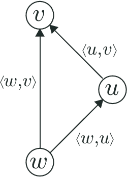
Figure 1: Triadic closure produced by user $w$’s copying of $u$’s follow link to $v$.

In Twitter, users very often find new information sources by browsing the friend lists of their friends and copying some of them which seem interesting to them. This kind of practice is not specific to Twitter, and is quite common to many social media. It is one of key differences between social media and other older media, such as RSS (RDF Site Summary or Really Simple Syndication) [3], where users cannot browse other users’ subscription. We also think it is one of the feature that promoted the growth of social media like Twitter over the older media. In addition, in Twitter, users can “retweet” (i.e., forward) a tweet from their friends to their followers, and when users find a tweet retweeted by a friend interesting to them, they often create direct follow links to the account that originally posted the tweet. Similar forwarding functions are found in many social media.

These observations are the rationale of our assumption that link propagation mainly occurs from users to their followers. Inclusion of other kinds of link propagation or link creation into the model is an interesting direction for future research.

In order to further narrowing down the candidates of links created by imitation, we also consider three other factors: time order of link creation, link reciprocity, and the similarity between users.

The first factor is time order of link creation. In a triadic closure, the link created by copying must be newer than the other two links. Otherwise, it must not be a result of copying.

The second factor, reciprocity of links, is used for distinguishing links to information sources and links between personal friends. In Twitter, non-reciprocal links are more likely to refer to information sources than reciprocal links are [19]. Because links to information sources are more important for the discovery of early adopters, we distinguish the two types of links based on their reciprocity.

Figure 2: The follow link from $w$ to $v$ is a part of many triadic closures and it is not obvious who in $u_{1},\ldots,u_{n}$ was imitated by $w$.

Even if we find a triadic closure and the links in it satisfy the conditions above, the candidate link in it may not actually be a copy of the link in that triad. If the candidate link is also a component of many other triadic closures, it may be a copy of another link in another triadic closure. Figure 2 illustrates such a situation. In this example, the follow link from the user $w$ to the user $v$ is a part of many triadic closures, and it is not obvious who in $u_{1},\ldots,u_{n}$ was imitated by $w$.

We estimate the probability that a candidate link is a copy of the link in a given triad by using similarity between interests of users in the triad. This is the third factor. This factor is based on an assumption that link propagation is more likely to happen when the interests of related users are similar to each other. We measure the similarity of interests of users by the similarity of their friend lists.

We use these three factors as optional factors, and tested all eight combinations of them in our experiments. Our experimental result shows that the link reciprocity is very useful for improving the accuracy of our method, but the other two are not very useful. The details will be explained later.

Notice that all information used by our method, network structure and the three optional factors explained above, can be obtained easily only by crawling the neighbors of the target new accounts in the current Twitter graph structure. This is one important advantage of our method.

In Twitter, link propagation to followers is especially likely to occur when users receive interesting messages retweeted by their friends. Our method, however, does not use the information on retweeting because it requires monitoring of the tweet stream, and we would lose the advantage of our method mentioned above.

By using network structure and the three optional factors above, we infer which links are copies of which links, and we estimate how many times each user has been imitated by other users. Based on this value, we compute early adopter score of each user. We then compute future popularity score of each account based on the early adopter scores of its followers.

1.3 Comparison with Baseline Methods

We conducted an experiment with a data set consisting of a part of Twitter graph that were collected by a random crawler on May 2012 [10]. We estimated future popularity of then-new accounts in this data set, and compared the result with the number of non-reciprocal followers that the accounts currently have as of May 2015, which indicates how popular these accounts are now. The result of the experiment shows that our method outperforms various baseline methods when we compare the accuracy of the whole ranking of all the new accounts. Our method outperforms baseline methods especially when we apply them to new accounts that have only a few followers.

In addition, the correlation between the ranking by our method and those by baseline methods are low. This suggests that our method and baseline methods are complementary to each other. Our experimental results shows that we can actually produce a even better ranking by logistic regression combining our method and some of the baseline methods.

When we compare the accuracy of only the top part of the rankings, a variation of HITS algorithm [8] or a variation of PageRank method [13] achieves the highest accuracy in most cases. Even a naive method that ranks the accounts by the number of the non-reciprocal followers they had at that time ourperforms our method in some cases. It is mainly because the top part of the rankings include accounts that were already popular in the old snapshot. This fact again suggests that our method is particularly useful when we want to find new accounts that are not popular now but will be popular in future.

Although our main purpose is to predict future popularity of new accounts, we also expect that analysis of early adopters discovered by our method would also help revealing what factors are important for new accounts to obtain links from early adopters, and what factors are important for users to be good early adopters.

2 Related Work

In sociology, there has been extensive research on the behavior of people in the real world. The results of the research are also helpful for understanding the behavior of people on social media. There have been some studies that have shown that the behavior reported in the past research in sociology is also observed on social media [7, 12, 6, 15]. One of such studies on the behavior of people has proposed the concept of triadic closure for explaining how people behave when they connect to each other. Our method uses this concept for inferring which links are created by copying which links.

Recently, there have also been many studies on link prediction in online social network. For example, Liben-Nowell and Kleinberg [11] was the first to formulate the problem of link-prediction on social network and they proposed a prediction method based on the proximity of nodes in the network. Zhang et al. [20] proposed a method that estimates the probability of future links by inferring latent paths of link propagation in the network. They estimate how important each node is as a mediator of link propagation by using a probabilistic model. Our method is based on a similar concept of early adopters. Their method, however, requires multiple snapshots of the network structure at different time point. On the other hand, our method for estimating the future popularity of a given account only requires information that can be obtained by crawling the neighbors of the target account in the current snapshot of the network structure. This is one big advantage of our method.

There have also been many studies on estimation of the influential power of nodes in social network. For example, Kwak et al. [9] compared three indicators, PageRank, the number of followers, and the number of retweets, for the estimation of popularity of Twitter accounts, and they showed that there is a discrepancy between the number of followers of an account and the popularity of tweets by the account, which suggests that the number of followers is not an only major factor of influential power of nodes. Weng et al. [18] also proposed a method for estimating influential power of Twitter accounts. Their method is based on the number of followers, but they also consider the interests of the followers and compute the probability that each tweet is actually read by the followers. These two studies focus on influential power of information sources in information dissemination, while the early adopter score used in our method indicates the influential power of nodes in link propagation.

The discovery of early adopters in online community has been discussed in several studies. Bakshy et al. [2] analyzed how users adopt new contents in a social network in Second Life, and identified early adopters, but also found that early adopters do not always have significant influence on the other users. Saez-Trumper et al. [16] proposed a method of identifying early adopters that also have significant influence on the others in information network, such as Twitter, and called such users trendsetters. These studies focused on temporal relationship of users’ adoption of contents, such as hashtags and URLs. Goyal et al. [5] also proposed a method of identifying leaders in online communities whose actions, e.g., tagging resources or rating songs, are imitated by many users. On the other hand, we focused on the adoption of new Twitter accounts, i.e., the creation of new follow links, and imitation of them by the followers. We showed that the idea similar to theirs can also be applied to such a type of actions in order to predict future popularity of new accounts in Twitter. Another contribution of this paper is to develop a method of inferring who copied which follow links, the information which is not immediately available.

3 Scores for Prediction

In this section, we define future popularity scores of accounts, which we use for ranking new accounts based on its prospective popularity, and also define early adopter scores of accounts, which we use for computing future popularity scores of their friends. We first define notation used in this paper. Let $G(V,E)$ be the follow graph of Twitter, where $V$ is a set of all Twitter accounts, and $E$ is a set of all follow links among them. $\langle u,v\rangle\in E$ denotes a follow link from a user $u$ to a user $v$. For $u\in V$, $\mathit{Friends}(u)$ denotes the set of users followed by $u$, and $\mathit{Followers}(u)$ denotes the set of followers of $u$. Similarly, $\mathit{Friends}(S)=\bigcup_{u\in S}\mathit{Friends}(u)$ and $\mathit{Followers}(S)=\bigcup_{u\in S}\mathit{Followers}(u)$.

3.1 Early Adopter Score: $E$

We first define early adopter scores of accounts. Let $\mathit{Copy}(u)$ denote a set of links $\langle w,v\rangle$ which a user $w$ who is a follower of $u$ created by copying a link $\langle u,v\rangle$. Figure 1 illustrates an example of such a link structure. $|\mathit{Copy}(u)|$ takes its maximum value when all followers of $u$ imitated all links by $u$. Therefore, $|\mathit{Copy}(u)|\leq|\mathit{Followers}(u)|\times|\mathit{Friends}(u)|$. We then define $I(u)$, the imitation ratio of $u\in V$, as follows.

Definition 1

The imitation ratio of $u$:

$$I(u)=\frac{|\mathit{Copy}(u)|}{|\mathit{Followers}(u)|\times|\mathit{Friends}(u)|}$$

The numerator is the number of times $u$ was imitated by its followers. The denominator is the maximum value that the numerator can take. When the denominator is $0$, we let $I(u)=0$. $I(u)$ represents the probability that a link of $u$ is imitated by its followers. How to infer $\mathit{Copy}(u)$ based on network structure and three optional factors will be explained later.

Based on $I(u)$, we define the early adopter score of $u$. We define it in two ways, and compare their performance by the experiment later. Both definitions try to estimate the expected number of link propagation through $u$, but they are based on different assumptions.

The first definition is based on the following assumption. Suppose a new information source $v$ is newly followed by an early adopter $u$. We then expect that each of the follower of $u$ will follow $v$ independently in the probability $I(u)$. Therefore, the expected number of new follow links created by imitating $u$ is $|\mathit{Follower}(u)|\times I(u)$.

However, we predict future popularity of an account based on the current snapshot. Even if a recently created account $v$ is followed by an account $u$ in the snapshot, if most followers of $u$ already have links to $v$ in the snapshot, we cannot expect that many users will newly follow $v$ by imitating $\langle u,v\rangle$. In other words, $u$ is not an “early adopter” compared with its followers with respect to $v$. With including this factor in the computation, we define $E_{1}(u,v)$, the first variation of an early adopter score of $u$ with respect to $v$, as follows.

Definition 2

The early adopter score of $u$ with respect to $v$ (variation 1):

$$E_{1}(u,v)=I(u)\times|\mathit{Followers}(u)\setminus\mathit{Followers}(v)|$$

This represents the expected increase of the number of followers of $v$ through $u$.

The second definition of the early adopter score of $u$ is based on the following assumption. Suppose an information source $v$ is followed by an early adopter $u$ in the current snapshot. Some of the followers of $u$ already have links to $v$. The other followers of $u$ are not likely to follow $v$ from now because they have not done so until now. However, the new followers that $u$ will obtain from now will follow $v$ by imitating $u$ in the probability $I(u)$. The number of followers that $u$ will obtain from now are unknown, and we simply assume that it is a constant $n$ for any $u$. Under this assumption, the expected increase of the number of followers of $v$ through $u$ is $n\times I(u)$. Because we use early adopter scores for computing ranking scores of accounts, we can ignore the constant $n$, and we define the second variation of the early adopter score as follows.

Definition 3

The early adopter score of $u$ (variation 2):

$$E_{2}(u,v)=I(u)$$

The second parameter $v$ of $E_{2}(u,v)$ is used only for the compatibility with the first variation $E_{1}(u,v)$, and is not actually used in this second variation.

There is another way to interpret $E_{2}(u,v)$. $I(u)$ represents how good $u$ is as an early adopter. If a new account $v$ is followed by a good early adopter, we can expect that the quality of $v$ is high, and therefore, we can expect that it will have many followers in future, no matter these new followers would find $u$ through $v$ or not. Therefore, we can simply use $I(u)$ for computing future popularty scores of accounts followed by $u$.

3.2 Future Popularity Score: $F$

By using the early adopter score defined above, we next define the future popularity score of an account $v$. The simplest way to define it is to sum up the early adopter scores of all the followers of $v$:

Definition 4

Sum-based future popularity score of $v$:

$$F_{i}^{\Sigma}(v)=\sum_{u\in\mathit{Followers}(v)}E_{i}(u,v)$$

where $i$ is either 1 or 2. This definition, however, has a problem when we use $E_{1}$. $E_{1}(u,v)$ represents the expected increase of the followers of $v$ through $u$, and if $u_{1}$ and $u_{2}$ have some common followers, simply summing up $E_{1}(u_{1},v)$ and $E_{1}(u_{2},v)$ would double-counts those common followers. Therefore, we should define $F_{1}^{\Sigma}(v)$ in the following way:

Definition 5

Sum-based future popularity score of $v$ (the second definition):

$$F_{1}^{\Sigma}(v)=\sum_{w\in\mathit{Followers}(\mathit{Followers}(v))}P(\bigvee_{u\in\mathit{Followers}(v)}cp(w,\langle u,v\rangle))$$

where $P(e)$ is the probability of the event $e$ and $cp(w,\langle u,v\rangle)$ is the event that $w$ copies the link $\langle u,v\rangle$. That is, we sum up the probability that a follower $w$ of some follower of $v$ will follow $v$ by imitating any of the followers of $v$. We compute this probability by assuming that events $cp(w,\langle u_{i},v\rangle)$ and $cp(w,\langle u_{j},v\rangle)$ are independent for $i\neq j$ and $P(cp(w,\langle u,v\rangle))=I(u)$. According to our experiment, however, the performance of $F_{1}^{\Sigma}(v)$ in this definition and that of the previous simpler definition have no significant difference. Therefore, we use the previous simpler definition for both $F_{1}^{\Sigma}(v)$ and $F_{2}^{\Sigma}(v)$.

A disadvantage of these sum-based definitions of future popularity scores is that it basically gives higher scores to accounts with many followers. Our purpose is to evaluate future popularity of new accounts that have not obtained many followers. Giving higher scores to accounts that already have many followers contradicts to our purpose.

Another way to define future popularity scores with avoiding that problem is to use g-index [4] instead of sum in the following way.

Definition 6

G-index-based future popularity score of $v$:

$$F_{i}^{g}(v)=\mbox{RG}(\{E_{i}(u,v)\ |\ u\in\mathit{Followers}(v)\})$$

where $i$ is either $1$ or $2$ and $\mbox{RG}(S)$ is a function that computes the rational g-index of the set of real numbers $S$ [17].

$F_{i}^{g}(v)$ is a rational g-index of the set of the early adopter scores of the followers of $v$. Given a set $S$ of values, its g-index can be computed by the following procedure. First we make a list $L$ by sorting values in $S$ in decreasing order. Let $L[i]$ be the $i$-th value in $L$. We then find a maximum $g$ that satisfies $g^{2}\leq c\times\sum_{i\leq g}L[i]$, where $c$ is a parameter, and such a $g$ is the g-index of $S$. G-index of a set $S$ is affected only by largest values in $S$. G-index of a set only takes natural numbers, but rational g-index is an extension of g-index to rational numbers [17].

4 Detection of Link Imitations

In the previous section, we defined early adopter score and future popularity score. In order to compute these scores, however, we first need to know $\mathit{Copy}(u)$, i.e., the set of links created by imitating a link from $u$. This information is not immediately available from Twitter data. In this section, we propose a method to estimate $|\mathit{Copy}(u)|$, i.e., the number of times such imitation has occurred. As explained in Section 1, we use network structure and the following three optional factors for it:

• temporal order of creation of links

• link reciprocity

• similarity among interests of users

4.1 Network Structure

Network structure is the most basic information for collecting candidates of links created by imitation. In this paper, we assume a user copies follow links only from his/her friends. On this assumption, if a link $\langle w,v\rangle$ is a copy of $\langle u,v\rangle$, there must also be a link $\langle w,u\rangle$, i.e., they must form a triangle shown in Figure 1. We call such a triangle triadic closure [14]. We first find such triadic closures.

We define a boolean function $\mathit{Structure}(u,v,w)$ that determines if $u,v,w\in V$ form a triangle that could be a triadic closure as follows:

Definition 7

Function determining if $u,v,w\in V$ of $G(V,E)$ forms a valid triangle:

$$\mathit{Structure}(u,v,w)=(\langle u,v\rangle\in E)\land(\langle v,w\rangle\in E)\land(\langle w,u\rangle\in E)$$

4.2 Time Order of Link Creation

Triangles satisfying the condition above do not necessarily correspond to triadic closures. We can further narrow down the candidates of triadic closures by using three optional factors. The first factor is temporal order of creation of links. In the triangle satisfying the condition above, $\langle w,v\rangle$ must be newer than $\langle u,v\rangle$ and $\langle w,u\rangle$ if $w$ created it by copying $\langle u,v\rangle$.

This information can be retrieved from the current Twitter data. Twitter API provides functions that return a list of followers and a list of friends of a given user. These functions return lists sorted by time when they became followers or friends from the newest one to the oldest one. Let $idx(v,l)$ denotes the position of $v$ in the list $l$. A boolean function representing whether the triangle satisfies the necessary temporal condition is then defined as follows:

Definition 8

Condition on temporal order of creation of links in a candidate triangle consisting of $u,v,w\in V$:

$$\mathit{Time}(u,v,w)=$$

$$idx(v,\mathit{Friends}(w))<idx(u,\mathit{Friends}(w))\ \land$$

$$idx(w,\mathit{Followers}(v))<idx(u,\mathit{Followers}(v))$$

Figure 3 illustrates examples of valid triangle (left) and invalid triangle (right). It also shows how we can check the conditions by the positions of $u$, $v$, $w$ in $\mathit{Friends}(w)$ and $\mathit{Followers}(v)$.

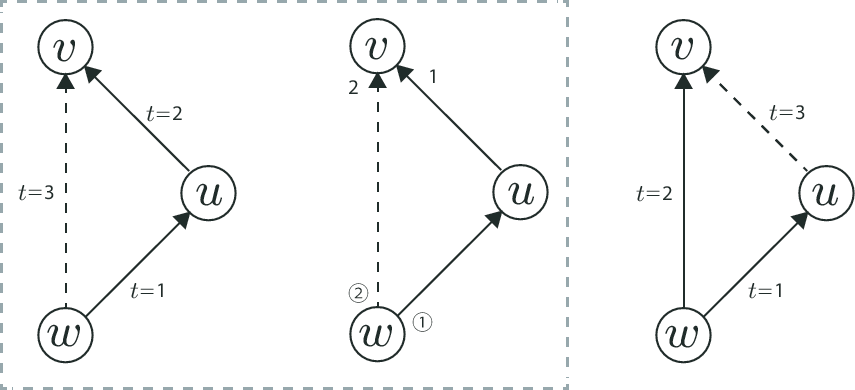
Figure 3: In the triad at left, $\langle w,v\rangle$ may be a copy of $\langle u,v\rangle$, but in the triad at right, $\langle w,v\rangle$ never be. The condition can be determined by the order of $u,v$ in the friend list of $w$ and the order of $u,w$ in the follower list of $v$, as shown at middle.

One disadvantage of this optional condition is that we need to store the time order of friends of $w$ and followers of $v$. In addition, surprisingly, this condition does not improve the performance of our method much, as explained later in Section 5.

4.3 Reciprocity of Links

Follow links in Twitter can be classified into several types, such as links to information sources and links to personal friends. There is also a practice called followback. In Twitter, some users follow back to many of its followers as an act of courtesy. Among these three types of links, the latter two are usually reciprocal. Personal friends usually link to each other [19], and links created by followback are always reciprocal. On the other hand, links to information sources are usually non-reciprocal unless the information source is a type of users who always follow back to all its followers.

In the following, $\mathit{Followers_{nr}}(u)$ denotes the set of non-reciprocal followers of $u$, i.e., $\mathit{Followers_{nr}}(u)=\mathit{Followers}(u)\setminus\mathit{Friends}(u)$. Similarly, $\mathit{Friends_{nr}}(u)$ denotes the set of non-reciprocal friends, $\mathit{Friends_{nr}}(u)=\mathit{Friends}(u)\setminus\mathit{Followers}(u)$.

For the discovery of early adopters, links to information sources are important. Therefore, we should exclude the other types of links from the consideration in our method. Although it is difficult to fully distinguish links to information sources from the others, we may be able to improve the precision of our method by excluding (or by giving lower weights to) reciprocal links because it excludes most of the other types of links (while it also excludes some links to information sources). Our experimental result, which will be shown in Section 5, shows that we can actually improve the precision by excluding reciprocal links.

Based on the discussion above, we define $\mathit{Nonrec}(u,v,w)$, the weight of the triad consisting of $u,v,w$, by the formula below:

Definition 9

The weight given to a triad of $u,v,w$:

$$\mathit{Nonrec}(u,v,w)=v\in\mathit{Friends_{nr}}(u)$$

In this paper, we simply assign the weight 0 to triads that have reciprocal links between $w$ and $v$. In other words, we exclude reciprocal links from the candidates of links created by imitation. Figure 4 illustrates this condition. By this factor, we expect that we can distinguish triadic closures corresponding to a circle of personal friends and those corresponding to imitation of links of early adopters.

Figure 4: Exclusion of reciprocal links from candidates.

4.4 Similarity between Interests of Users

By using the three conditions above, we can narrow down candidate triads corresponding to link imitation. However, if there are multiple candidates of the original link for one link, only one of them was really copied. When we have such multiple candidates, instead of selecting one of them as the original link, we assign each of them the probability that it is really the imitated one.

The simplest way to assign the probability is to assign equal probability to all the candidates. We also designed another way to assign probability that is proportional to the similarity between interests of users, which is the third optional factor.

In Twitter, various users with various interests publish or collect information. Early adopters must also have some specific interests, and each early adopter must be good at finding new useful information only on some topics. Similarly, users imitating early adopters also have some specific interests, and they are more likely to imitate early adopters that have interests similar to theirs. We compute weights given to each candidates based on these assumptions.

For example, suppose $w$ created a link to $v$, and there are multiple candidate users $u_{1},\ldots u_{n}$ as the user imitated by $w$. Figure 2 illustrates this situation. If the interests of $u_{i}$ and $v$ are very similar, $v$ is likely to be an information source on a topic for which $u_{i}$ is a good early adopter. Similarly, if the interests of $w$ and $u_{i}$ are similar, $w$ is more likely to imitate $u_{i}$ than other $u_{j}$ whose interests are not similar to interests of $w$.

We measure similarity between interests of two users by the similarity of their sets of friends. Similarity between $u,v\in V$, denoted by $\mathit{Sim}(u,v)$, is defined as follows:

Definition 10

Similarity between interests of $u$ and $v$:

$$\mathit{Sim}(u,v)=\frac{|\mathit{Friends}(u)\cap\mathit{Friends}(v)|}{|\mathit{Friends}(u)\cup\mathit{Friends}(v)|}$$

The details of how to assign weighted probability to candidates is explained in Section 4.5.

4.5 Estimation of Imitation Frequency

Now we explain how we estimate $|\mathit{Copy}(u)|$, imitation frequency of a user $u$, with including network structure and the three optional factors above. We first estimate the probability that a follow link $\langle w,v\rangle$ was created by imitating the link $\langle u,v\rangle$, denoted by $P_{\langle w,v\rangle}(u)$, by the formula below:

Definition 11

The probability that the link $\langle w,v\rangle\in E$ is a copy of $\langle u,v\rangle\in E$:

$$P_{\langle w,v\rangle}(u)=\frac{p_{\langle w,v\rangle}(u)}{\sum_{x\in V}p_{\langle w,v\rangle}(x)}$$

where

$$\begin{split}p_{\langle w,v\rangle}(x)=&\mathit{Structure(x,v,w)}\times\mathit{Time(x,v,w)}\times\\ &\mathit{Nonrec}(x,v,w)\times\mathit{Sim}(x,v)\times\mathit{Sim}(w,x)\end{split}$$

The formula above corresponds to the case where we use all three optional factors. When we do not use some of them, we simply remove terms corresponding to them from the formula. The Boolean values of $\mathit{Structure}(x,v,w)$, $\mathit{Time}(x,v,w)$, and $\mathit{Nonrec}(v,u,w)$ are interpreted as 1 or 0, and they are used to give the score 0 to accounts that cannot be the one that were imitated. $\mathit{Sim}(x,v)$ and $\mathit{Sim}(w,x)$ are used to give proper weights to multiple candidates.

We then estimate $|\mathit{Copy}(u)|$, required for the computation of the final early adopter scores, as follows:

Definition 12

$\mathit{CF}(u)$, the expected value of $|\mathit{Copy}(u)|$:

$$\mathit{CF}(u)=\sum_{\langle w,v\rangle\in E}P_{\langle w,v\rangle}(u)$$

We estimate the expected value of the number of times $u$ was imitated by summing the probability that each candidate link is a copy of the link of $u$.

4.6 Algorithms

We have designed two algorithms to compute early adopter scores of the followers of the given new accounts. The first one computes early adopter scores of all accounts in the graph by exactly following the definition above. For each follow link in the given graph, we collect candidate links that can be the original of the link, and give the owner of each link the probability that it is the original. At each account, these given probabilities are accumulated. By summing up all these probability values given to a user $u$, we obtain the expected value of $|\mathit{Copy}(u)|$. This algorithm is shown in Algorithm 1.

This algorithm evaluates $c_{\langle w,v\rangle}(u)$ for $O(md)$ times where $m$ is the number of edges in the graph and $d$ is the degree of nodes. When we use no optional factors, we actually do not need to compute $c_{\langle w,v\rangle}(u)$ in Algorithm 1 because it always returns 1 given that $\langle w,v\rangle\in E$ and $u\in\mathit{Followers}(v)\cap\mathit{Friends}(w)$. Therefore, the time complexity of this algorithm is in $O(md)$ in that case, if we assume $\mathit{Followers}(u)$ and/or $\mathit{Friends}(u)$ are stored in a hash table. Even if we include the factor $\mathit{Nonrec}$, we can simply skip the loop for such $\langle w,v\rangle$, and the complexity of the algorithm is still in $O(md)$. According to our experiments, which will be explained later, the other two factors are not actually useful, so the time complexity of our best method is in $O(md)$.

Algorithm 1 Computing Early Adopter Scores of All Nodes

  $\mathit{CF}(u):=0$ for all $u\in V$

  for all $\langle w,v\rangle\in E$ do

     $U:=\mathit{Followers}(v)\cap\mathit{Friends}(w)$

     $s:=0$

     for all $u\in U$ do

        $c[u]:=c_{\langle w,v\rangle}(u)$

        $s:=s+c[u]$

     end for

     for all $u\in U$ do

        $CF(u)=CF(u)+c[u]/s$

     end for

  end for

  return  $CF(u)$ for all $u\in V$

The algorithm above computes early adopter scores for all nodes, but when we only want to compute a future popularity score of one new account, we only need to compute early adopter scores of its followers. For such cases, we designed another algorithm to compute the early adopter score of a given user $u$. We omit the details, but it simply collects all candidate triadic closures by retrieving all the friends of the followers of $u$, and checking if they are friends of $u$. Its time complexity is in $O(d^{3})$, and therefore we can compute the future popularity score of a given account in $O(d^{4})$. According to our experiment, however, this algorithm can be slower even when we need to compute early adopter scores only for less than a thousand of nodes.

4.7 Extension to a Recursive Method

The method explained above computes the future popularity score of an account based on the early adopter scores of its direct followers. We can easily extend this method to a recursive method based on various infection models.

As explained before, $E_{1}(u,v)$ represents the expected number of link propagation from $u$ to its followers and $E_{2}(u,v)$ represents the probability that links are propagated from $u$ to its followers. We can interpret them as the propagation probability of a disease, and can run some algorithms that predict how many users will be infected starting from a given infected user. We tested such recursive versions of our method by using some simple algorithms, in our experiment, such recursive method did not improve the performance of our method. We will investigate this problem in our future research.

5 Experiment

In this section, we evaluate our method by the experiment on the Twitter data set. We first explain the data set used in our experiment and the procedure of our experiment. After that, we will explain the baseline methods with which we compared our methods. Finally, we show and discuss the results of the experiment.

5.1 Data Set

We use the snapshot of a part of Twitter follow graph created by Rui et al. in May 2011 [10]. This data set was produced by random crawling of follow links starting from randomly selected 100,000 users. In this graph, $|V|=21,604,165$ and $|E|=284,885,001$. We denote this network by $D_{11}(V,E)$ in order to distinguish it from another network explained later.

We extracted all accounts in $D_{11}$ that were within two weeks, three weeks, and four weeks from its creation date, and that had at least 10 followers, 20 followers, and 30 followers at the time of $D_{11}$. Let $T^{2}_{10}$, $T^{2}_{20}$, $T^{2}_{30}$, $T^{3}_{10}$, $T^{3}_{20}$, $T^{3}_{30}$, $T^{4}_{10}$, $T^{4}_{20}$, $T^{4}_{30}$ denote these data sets. Therefore, $T^{x}_{30}\subseteq T^{x}_{20}\subseteq T^{x}_{10}$ and $T^{2}_{x}\subseteq T^{3}_{x}\subseteq T^{4}_{x}$. Their size is shown at the top of Table 1.

5.2 Procedure of Experiment

We run our experiment in the following procedure:

1. For all accounts in the data set, we estimated their future popularity by our methods and by various baseline methods, and produce a list of accounts sorted in the order of their estimated future popularity.

2. We used the number of their non-reciprocal followers as of May 2015, which we denote $\mbox{FW}_{\mathit{nr}}^{2015}(u)$, as the true future popularity of the information sources, and produce a list of accounts sorted in that order.

3. We compare the list produced by each estimation method and the list based on $\mbox{FW}_{\mathit{nr}}^{2015}(u)$. For the comparison, we used Spearman’s rank correlation coefficient ($\rho$) and the normalized discount cumulative gain (nDCG). Spearman’s $\rho$ reflects the accuracy of the whole estimated ranking, while nDCG only reflects the accuracy of the top part of the estimated ranking.

data set			$T^{4}_{10}$	$T^{3}_{10}$	$T^{2}_{10}$	$T^{4}_{20}$	$T^{3}_{20}$	$T^{2}_{20}$	$T^{4}_{30}$	$T^{3}_{30}$	$T^{2}_{30}$	$\hat{T}^{4}_{10}$	$\hat{T}^{3}_{10}$	$\hat{T}^{2}_{10}$	$\hat{T}^{4}_{20}$	$\hat{T}^{3}_{20}$	$\hat{T}^{2}_{20}$
data size			6921	3270	1515	2259	1005	431	979	396	165	2249	1009	415	709	314R	123
	FW		0.18	0.20	0.23	0.15	0.12	0.07	0.19	0.18	0.00	0.19	0.19	0.19	0.20	0.20	0.19
	$\mbox{FW}_{\mathit{nr}}$		0.11	0.07	0.08	0.02	0.01	-0.01	0.00	-0.03	-0.01	0.07	0.10	0.08	0.00	0.03	-0.03
	FR		0.19	0.25	0.31	0.24	0.20	0.22	0.33	0.30	0.35	0.26	0.24	0.23	0.34	0.37	0.53
	$\mbox{FR}_{\mathit{nr}}$		0.04	-0.05	-0.04	-0.05	0.01	0.04	-0.05	-0.04	-0.05	0.02	0.09	0.13	-0.09	0.02	0.08
	HITS		0.15	0.11	0.10	0.11	0.13	0.10	0.04	0.07	0.08	0.13	0.16	0.12	0.12	0.11	0.02
	$\mbox{HITS}_{\mathit{nr}}$		0.26	0.27	0.31	0.30	0.30	0.35	0.38	0.38	0.46	0.33	0.31	0.33	0.41	0.45	0.61
	PR		0.20	0.15	0.13	0.20	0.15	0.14	0.24	0.19	0.25	0.16	0.14	0.14	0.21	0.19	0.26
	$\mbox{PR}_{\mathit{nr}}$		0.16	0.12	0.09	0.21	0.17	0.20	0.30	0.27	0.32	0.21	0.19	0.22	0.30	0.35	0.51
	$\mbox{AD}_{\Sigma}$		-0.06	-0.08	-0.08	-0.17	-0.21	-0.27	-0.18	-0.24	-0.26	-0.12	-0.10	-0.15	-0.22	-0.28	-0.40
	$\mbox{AD}_{\mu}$		-0.21	-0.17	-0.13	-0.30	-0.38	-0.46	-0.27	-0.37	-0.50	-0.27	-0.31	-0.31	-0.35	-0.50	-0.54
$F_{1}$	$\Sigma$	-	0.30	0.27	0.29	0.24	0.25	0.27	0.23	0.23	0.32	0.28	0.32	0.36	0.29	0.32	0.40
		r	0.36	0.35	0.38	0.32	0.32	0.38	0.34	0.36	0.46	0.35	0.36	0.39	0.38	0.42	0.57
		s	0.30	0.26	0.28	0.24	0.25	0.27	0.21	0.22	0.31	0.28	0.32	0.36	0.28	0.31	0.42
		r s	0.35	0.33	0.36	0.29	0.30	0.36	0.32	0.33	0.44	0.32	0.33	0.38	0.34	0.38	0.55
	g	-	0.30	0.28	0.31	0.27	0.27	0.31	0.25	0.24	0.35	0.29	0.31	0.36	0.31	0.34	0.43
		r	0.35	0.34	0.37	0.31	0.32	0.36	0.33	0.35	0.46	0.35	0.35	0.38	0.36	0.41	0.53
		s	0.30	0.28	0.30	0.27	0.27	0.30	0.24	0.22	0.29	0.29	0.31	0.37	0.30	0.33	0.44
		r s	0.35	0.32	0.35	0.31	0.32	0.37	0.32	0.33	0.43	0.33	0.33	0.37	0.35	0.37	0.52
$F_{2}$	$\Sigma$	-	0.39	0.37	0.39	0.36	0.37	0.42	0.34	0.32	0.40	0.39	0.40	0.44	0.44	0.50	0.62
		r	0.39	0.39	0.41	0.39	0.39	0.45	0.40	0.38	0.47	0.39	0.39	0.43	0.46	0.52	0.64
		s	0.38	0.37	0.38	0.36	0.36	0.41	0.33	0.31	0.38	0.38	0.39	0.43	0.43	0.48	0.61
		r s	0.39	0.38	0.40	0.38	0.38	0.45	0.39	0.37	0.47	0.38	0.38	0.42	0.45	0.50	0.64
	g	-	0.38	0.36	0.37	0.35	0.36	0.39	0.31	0.30	0.37	0.42	0.45	0.47	0.43	0.49	0.58
		r	0.39	0.38	0.41	0.38	0.38	0.44	0.38	0.37	0.45	0.39	0.39	0.43	0.45	0.51	0.63
		s	0.38	0.36	0.36	0.35	0.36	0.40	0.31	0.31	0.38	0.42	0.45	0.47	0.42	0.46	0.58
		r s	0.39	0.38	0.40	0.38	0.38	0.44	0.38	0.36	0.45	0.38	0.39	0.42	0.45	0.50	0.63
LR			0.43	0.43	0.46	0.43	0.45	0.50	0.45	0.46	0.58	0.47	0.50	0.50	0.52	0.57	0.65

Table 1: Spearman’s $\rho$ between $\mbox{FW}^{2015}_{\mathit{nr}}$ and each method. FW to $\mbox{AD}_{\mu}$ are baseline methods, $F_{1}$ and $F_{2}$ are our methods, and $LR$ is the logistic regression combining some baseline methods and our methods. $T$ denotes data sets including both active and non-active users. $\hat{T}$ denotes data sets only including active users. For each data set, the best scores among the baseline methods and the best score among 16 variations of our method are shown in bold fonts. The best scores among both of them are also underlined. A variation of our method $F_{2}^{\Sigma}(r)$ outperforms the baseline methods except for $T^{2}_{20}$ and $T^{2}_{30}$. Notice that $F_{2}^{\Sigma}(r)$ outperforms the baseline methods even for $\hat{T}^{x}_{10}$, where the score of $F_{2}^{\Sigma}(r)$ are not in bold fonts simply because $F_{2}^{g}$ was the best among our methods.

5.3 Tested Proposed Methods

In Section 3, we showed two definitions of early adopter scores, $E_{1}(u,v)$ and $E_{2}(u,v)$, and we also showed two ways to calculate future popularity scores, $F_{i}^{\Sigma}$ and $F_{i}^{g}$. We also have three optional factors in the estimation of $|\mathit{Copy}(u)|$, and there are eight combinations of them. In total, we have 32 combinations of them and we compared them in our experiment. In this paper, however, we omit the result of the methods that use temporal order of links because it did not improve the accuracy of our method, and also because of the spece limitation.

In the following, $r$ denotes the option of link reciprocity, and $s$ denote the option of similarity between users. For example, $F_{2}^{\Sigma}(r)$ represents our method using $E_{2}(u,v)$, $F_{i}^{\Sigma}(v)$, and only link reciprocity option.

The parameter $c$ for g-index was hand-tuned to the following values in each case. $E_{1}$: 50000, $E_{1}+r$: 100000, $E_{1}+s$: 50000, $E_{1}+r,s$: 50000, $E_{2}$: 1, $E_{2}+r$: 10, $E_{2}+s$: 1, $E_{2}+r,s$: 10.

5.4 Baseline Methods

We next explain the baseline methods we compared and their parameters.

Followers (FW): It measures the future popularity of new accounts by the number of their current followers in May 2011.

Nonreciprocal followers ($\mbox{FW}_{\mathit{nr}}$): It measures it by the number of their non-reciprocal followers in May 2011. As explained in Section 4.3, non-reciprocal follow links are likely to be links to information sources.

Friends (FR): It measures it by the number of friends in May 2011.

Nonreciprocal friends ($\mbox{FR}_{\mathit{nr}}$): It measures it by the number of their non-reciprocal friends in May 2011.

HITS: It computes authority scores and hub scores of accounts [15], and use the authority score as the indicator of future popularity. In this experiment, we set the number of iterations to 10, with which the scores sufficiently converged.

Nonreciprocal HITS ($\mbox{HITS}_{\mathit{nr}}$): The same as HITS, but it computes authority and hub score on the graph consisting only of non-reciprocal links. The number of iterations is 10, with which the scores sufficiently converged.

PageRank (PR): It estimates the future popularity by using PageRank score [13]. In this experiment, we set the damping factor $d=0.9$ and number of iterations to 100, with which the scores sufficiently converged.

Nonreciprocal PageRank ($\mbox{PR}_{\mathit{nr}}$): The same as PageRank, but it computes PageRank scores on the graph consisting only of nonreciprocal links. We set the damping factor $d=0.9$ and the number of iterations is 100, with which the scores sufficiently converged.

Adamic/Adar ($\mbox{AD}_{\Sigma}$, $\mbox{AD}_{\mu}$): It estimates the future popularity of $v$ by estimating the probability of new links to $v$ from other nodes based on Adamic/Adar index [1]. Given an account $v$, we collect all its friends, and also all the followers of those friends. Then we compute Adamic/Adar index for $v$ and all these followers with regarding their common friends as the common items. The ordinary Adamic/Adar sums all the obtained index values, but we compared both summation and average.

5.5 Result and Discussion

We next analyze and discuss the results of our experiment.

We first analyze the correlation between the ranking lists based on $\mbox{FW}_{\mathit{nr}}^{2015}$ and each method by Spearman’s $\rho$. The left half of Table 1 lists the $\rho$ values between $\mbox{FW}_{\mathit{nr}}^{2015}$ and each method. In each column in Table 1, the best scores among the baseline methods and the best score among the 16 variations of our method are shown in bold fonts.

Among the baselines, FW and FR achieved higher correlation than those without reciprocal links. On the contrary, HITS and PR without reciprocal links achieved higher correlation than those with reciprocal links. Among them, $\mbox{HITS}_{\mathit{nr}}$ was the best, and $\mbox{PR}_{\mathit{nr}}$ follows. These methods have higher correlation for the data set including accounts with more followers.

On the other hand, AD methods have negative correlation, and AD_μ has, surprisingly, high negative correlation, which means it is a good index for predicting future popularity of accounts. It also has higher correlation for the data set including accounts with more followers.

However, our method, especially $F_{2}^{\Sigma}(r)$ achieves even higher correlation except for two cases for the data set $T^{2}_{20}$ and $T^{2}_{30}$. Our method is outperformed by AD_μ in these cases, where the data set includes accounts that have already obtained many followers (more than 20 or 30) within a short time (2 weeks). This suggests that our method is especially good at the discovery of accounts that start with a fewer followers, but then become popular later.

We performed some error-analysis, and the result shows that the main factor lowering the accuracy of all the compared methods is the existence of many accounts that had some followers in $D_{11}$ but are inactive or deleted as of 2015. Therefore, we also created data sets $\hat{T}$ that include only accounts that are active as of 2015. The right half of Table 1 shows the result on these data sets. In thes data sets, we again outperforms baselines, and achieves higher accuracy than for $T$, i.e., the data set including inactive users. This suggest that we should combine our method with some method that predict if a given account will last long or not. Notice that $F_{2}^{\Sigma}(r)$ outperforms the baseline methods in all cases although their scores are not in bold fonts in some cases where they are outperformed by $F_{2}^{g}$.

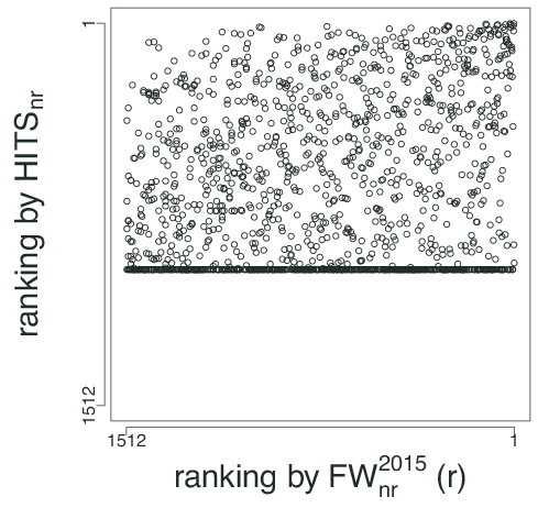
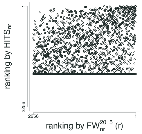
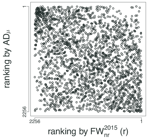
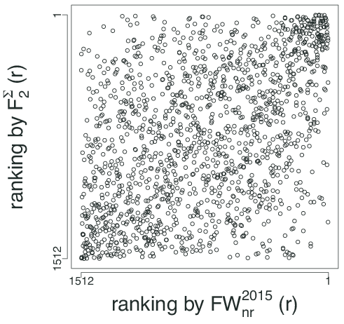
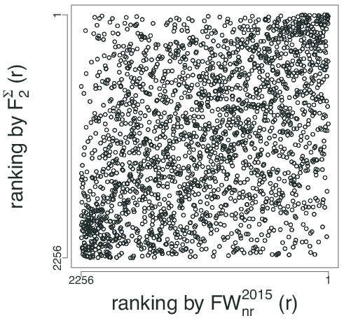
Figure 5: Scatter diagram for $\mbox{HITS}_{\mathit{nr}}$, $\mbox{AD}_{\mu}$, $F_{2}^{\Sigma}(r)$, which had high $\rho$ value, for $T^{2}_{10}$ (left) and $T^{4}_{20}$ (right). The horizontal row of points near the bottom in the daigram for $\mbox{HITS}_{\mathit{nr}}$ corresponds to the accounts that had no non-reciprocal followers in $D_{11}$.

Figure 5 show scatter diagrams between $\mbox{FW}_{\mathit{nr}}^{2015}$ and each method that showed high correlation, i.e., $\mbox{HITS}_{\mathit{nr}}$, $\mbox{AD}_{\mu}$, $F_{2}^{\Sigma}(r)$, for the data set $T^{2}_{10}$ (left) and $T^{4}_{20}$ (right). In the scatter diagrams for $\mbox{HITS}_{\mathit{nr}}$, there are a horizontal row of points near the bottom. They are accounts that had no non-reciprocal followers in $D_{11}$. The methods that use non-reciprocal links achieves higher $\rho$ values, but they also have this problem.

data set			$T^{4}_{10}$				$T^{3}_{10}$				$T^{2}_{10}$
nDCG@k			$@10$	$@20$	$@50$	$@100$	$@10$	$@20$	$@50$	$@100$	$@10$	$@20$	$@50$	$@100$
	FW		0.05	0.04	0.05	0.05	0.19	0.17	0.15	0.18	0.03	0.06	0.11	0.11
	$\mbox{FW}_{\mathit{nr}}$		0.08	0.15	0.14	0.16	0.07	0.07	0.14	0.15	0.17	0.17	0.18	0.18
	FR		0.02	0.02	0.03	0.03	0.17	0.15	0.14	0.14	0.01	0.01	0.03	0.05
	$\mbox{FR}_{\mathit{nr}}$		0.00	0.00	0.01	0.01	0.00	0.00	0.00	0.01	0.00	0.00	0.00	0.01
	HITS		0.00	0.02	0.02	0.03	0.11	0.10	0.09	0.10	0.01	0.01	0.02	0.03
	$\mbox{HITS}_{\mathit{nr}}$		0.19	0.19	0.18	0.19	0.13	0.14	0.18	0.20	0.25	0.27	0.29	0.30
	PR		0.07	0.07	0.07	0.13	0.23	0.24	0.23	0.24	0.12	0.12	0.17	0.20
	$\mbox{PR}_{\mathit{nr}}$		0.17	0.16	0.18	0.18	0.02	0.06	0.11	0.15	0.11	0.14	0.16	0.17
	$\mbox{AD}_{\Sigma}$		0.07	0.13	0.14	0.14	0.20	0.22	0.21	0.20	0.25	0.24	0.23	0.24
	$\mbox{AD}_{\mu}$		0.00	0.00	0.00	0.01	0.00	0.00	0.01	0.02	0.00	0.01	0.02	0.06
$F_{2}$	$\Sigma$	-	0.03	0.05	0.09	0.11	0.21	0.18	0.25	0.25	0.13	0.16	0.16	0.16
		r	0.00	0.00	0.00	0.00	0.00	0.00	0.00	0.00	0.00	0.00	0.01	0.06
		s	0.06	0.06	0.05	0.05	0.19	0.16	0.15	0.16	0.03	0.03	0.04	0.09
		r,s	0.06	0.13	0.14	0.15	0.12	0.14	0.17	0.17	0.22	0.21	0.20	0.22
	$g$	-	0.02	0.02	0.02	0.02	0.02	0.01	0.02	0.05	0.03	0.03	0.04	0.11
		r	0.06	0.11	0.13	0.14	0.07	0.10	0.13	0.15	0.16	0.19	0.18	0.19
		s	0.00	0.00	0.01	0.02	0.01	0.01	0.03	0.03	0.02	0.05	0.05	0.08
		r,s	0.05	0.04	0.04	0.04	0.03	0.03	0.03	0.03	0.03	0.03	0.03	0.03

Table 2: $\mbox{nDCG}@k$ by each methods where gain is $\mbox{FW}_{\mathit{nr}}^{2014}$. Each column shows values of $k$, and the bold entries are highest score among the baseline methods and among the variations of our method. The best scores among both of them are also underlined.

	FW	$\mbox{FW}_{\mathit{nr}}$	FR	$\mbox{FR}_{\mathit{nr}}$	HITS	$\mbox{HITS}_{\mathit{nr}}$	PR	$\mbox{PR}_{\mathit{nr}}$	$\mbox{AD}_{\Sigma}$	$\mbox{AD}_{\mu}$	$F_{2}^{\Sigma}$	$F_{2}^{\Sigma}(r)$	$F_{2}^{\Sigma}(s)$	$F_{2}^{\Sigma}(r,s)$
FW	1.00	0.16	0.69	0.18	0.57	0.13	0.32	0.19	0.65	0.31	0.52	-0.01	0.60	0.35
$\mbox{FW}_{\mathit{nr}}$		1.00	-0.08	0.03	0.15	0.82	0.12	0.87	-0.03	-0.08	0.08	-0.02	0.09	0.10
FR			1.00	0.71	0.57	-0.05	0.36	-0.03	0.78	0.27	0.47	0.11	0.51	0.36
$\mbox{FR}_{\mathit{nr}}$				1.00	0.32	0.05	0.25	0.04	0.47	0.06	0.21	0.14	0.20	0.22
HITS					1.00	0.07	0.35	0.16	0.64	-0.07	0.22	-0.11	0.30	0.05
$\mbox{HITS}_{\mathit{nr}}$						1.00	0.15	0.74	-0.15	-0.18	0.28	0.25	0.26	0.34
PR							1.00	0.12	0.20	-0.06	0.37	0.21	0.37	0.37
$\mbox{PR}_{\mathit{nr}}$								1.00	-0.04	-0.10	0.18	0.09	0.18	0.18
$\mbox{AD}_{\Sigma}$									1.00	0.46	0.02	-0.41	0.11	-0.12
$\mbox{AD}_{\mu}$										1.00	-0.08	-0.34	-0.02	-0.16
$F_{2}^{\Sigma}$											1.00	0.81	0.97	0.93
$F_{2}^{\Sigma}(r)$												1.00	0.71	0.85
$F_{2}^{\Sigma}(s)$													1.00	0.87
$F_{2}^{\Sigma}(r,s)$														1.00

Table 3: Spearman’s $\rho$ between each methods. Our best methods and the best baseline methods have low correlation, which suggests that they are complementary to each other.

In Figure 5, the diagram for $\mbox{AD}_{\mu}$ and $T^{4}_{20}$ shows that they are mainly good at distinguishing the least popular accounts while $F_{2}^{\Sigma}(r)$ is good at both the most popular accounts and the least popular accounts. In order to examine these aspects in more detail, we also compared baseline methods and our methods by the normalized discount cumulative gain (nDCG). nDCG is a measure of ranking quality, and takes value in the range of $[-1,1]$. In nDCG, accuracy of the top part of a ranking is more important than the lower part. nDCG@$k$ is a measure that computes nDCG only for top $k$ in the ranking. We calculated nDCG@$k$ of each method with various $k$ for some data set. Table 2 shows the result. The best scores among the baselines and those among our methods are shown in bold fonts, and the best score among both of them are also underlined.

Among the baselines, $\mbox{HITS}_{\mathit{nr}}$, $\mbox{PR}_{\mathit{nr}}$, and AD_μ have high scores for some cases. In this comparison, our method does not achieve as good performance as these baselines. It is mainly because top-ranked accounts were already popular at 2,3,4 weeks after the creation. This again suggests that our method is mainly good at detecting accounts that are not popular now but will be popular later.

We also calculated the correlation between our methods and baseline methods. Figure 3 shows the result. This result shows that there are very low correlation between the good baseline methods, such as $\mbox{HITS}_{\mathit{nr}}$ and $\mbox{AD}_{\mu}$, and our best methods. This suggest that we can achieve better performance by combining these methods. Following this observation, we tested the logistic regression combining the methods that showed high correlation in this experiment. We learned weight parameter for each combined method and evaluated their results by 10-fold validation. Table 4 shows the result. Both $F_{1}^{\Sigma}$ and $F_{2}^{\Sigma}$ were given high $\beta$ values, which means they highly contribute the result. All $p$ values are small enough, which shows this result is stasistically reliable.

The accuracy of this combined method is shown at the line LR at the bottom of Table 1. This method achieves the best accuracy in all cases.

Method	$\beta$	$p$
$(Intercept)$	-1.23115	$<2.0\times 10^{-16}$
HITS	0.46882	$1.21\times 10^{-6}$
$\mbox{HITS}_{\mathit{nr}}$	1.13858	$1.21\times 10^{-11}$
$\mbox{AD}_{\mu}$	-1.01902	$<2.00\times 10^{-16}$
$F_{1}^{\Sigma}r$	0.99312	$5.77\times 10^{-15}$
$F_{2}^{\Sigma}r$	0.98678	$2.40\times 10^{-11}$

Table 4: Result of logistic regression LR for $T^{4}_{10}$. Both $F_{1}^{\Sigma}r$ and $F_{2}^{\Sigma}r$ highly contribute to the result.

6 Conclusion

In this paper, we proposed a method of predicting future popularity of new Twitter accounts. Our approach is based on the concept of early adopters. Early adopters are users that can find new useful information sources earlier than other users. Even if a new account currently has only a few followers, if the followers are good early adopters, we expect the new account will have many followers in future. We find early adopters based on the frequency of link imitation, i.e., how often their follow links are imitated by their followers. We, therefore, need information on who imitated which links in order to find early adopters, but that information is not immediately available from the current Twitter graph. We developed a method that infer it by using four factors: network structure, temporal order of creation of links, similarity between interests of users, and reciprocity of links.

We evaluated the performance of our approach by estimating future popularity of new Twitter accounts, and comparing the result with the number of followers they actually obtained later. The results show that our approach achieves higher accuracy in the prediction of future popularity of new information sources than various baseline methods. Our approach outperforms the baselines especially for users that were not popular at the time of prediction. It means our approach is more useful when we want to find new information sources that are not popular now but will be popular in future. Because the result of our method and the best baseline method have low correlation, we also tested logistic regression combining our method and the best baseline methods, and it achieves even higher accuracy.

In this paper, we focus on the identification of early adopters, but another interesting issue is what kind of properties these early adopters have, and what makes them good early adopters. In future work, we will analyze early adopters identified by our method, and clarify why they can find new good information sources earlier than others, and why they are imitated by many users.

References

- [1] L. Adamic and E. Adar. Friends and neighbors on the web. Social Networks, 25:211–230, 2001.
- [2] E. Bakshy, B. Karrer, and L. A. Adamic. Social influence and the diffusion of user-created content. In Proc. of ACM EC, pages 325–334, 2009.
- [3] T. R. A. Board. Rss 2.0 specification. http://www.rssboard.org/rss-specification.
- [4] L. Egghe. Theory and practice of the g-index. Scientometrics, 69(1):131–152, 2006.
- [5] A. Goyal, F. Bonchi, and L. V. Lakshmanan. Discovering leaders from community actions. In Proc. of CIKM, pages 499–508, 2008.
- [6] J. Hopcroft, T. Lou, and J. Tang. Who will follow you back?: reciprocal relationship prediction. In Proc. of CIKM, pages 1137–1146. ACM, 2011.
- [7] H. Hu and X. Wang. How people make friends in social networking sites—a microscopic perspective. Physica A: Statistical Mechanics and its Applications, 391(4):1877–1886, 2012.
- [8] J. M. Kleinberg. Authoritative sources in a hyperlinked environment. Journal of the ACM, 46(5):604–632, 1999.
- [9] H. Kwak, C. Lee, H. Park, and S. Moon. What is twitter, a social network or a news media? In Proc. of WWW Conf., pages 591–600. ACM, 2010.
- [10] R. Li, S. Wang, H. Deng, R. Wang, and K. C.-C. Chang. Towards social user profiling: unified and discriminative influence model for inferring home locations. In Proc. of KDD, pages 1023–1031, 2012.
- [11] D. Liben-Nowell and J. Kleinberg. The link-prediction problem for social networks. JASIST, 58(7):1019–1031, 2007.
- [12] V.-A. Nguyen, E.-P. Lim, H.-H. Tan, J. Jiang, and A. Sun. Do you trust to get trust? a study of trust reciprocity behaviors and reciprocal trust prediction. In Proc. of SDM, pages 72–83, 2010.
- [13] L. Page, S. Brin, R. Motwani, and T. Winograd. The PageRank citation ranking: Bringing order to the web. Technical Report 1999-66, Stanford InfoLab, November 1999. Previous number = SIDL-WP-1999-0120.
- [14] A. Rapoport. Spread of information through a population with socio-structural bias: I. assumption of transitivity. The bulletin of mathematical biophysics, 15(4):523–533, 1953.
- [15] D. M. Romero and J. M. Kleinberg. The directed closure process in hybrid social-information networks, with an analysis of link formation on twitter. In Proc. of ICWSM, 2010.
- [16] D. Saez-Trumper, G. Comarela, V. Almeida, R. Baeza-Yates, and F. Benevenuto. Finding trendsetters in information networks. In Proc. of SIGKDD, pages 1014–1022, 2012.
- [17] R. S. Tol. A rational, successive g-index applied to economics departments in ireland. Journal of Informetrics, 2(2):149–155, 2008.
- [18] J. Weng, E.-P. Lim, J. Jiang, and Q. He. Twitterrank: finding topic-sensitive influential twitterers. In Proc. of WSDM, pages 261–270, 2010.
- [19] W. Xie, C. Li, F. Zhu, E.-P. Lim, and X. Gong. When a friend in twitter is a friend in life. In Proc. of WebSci, pages 344–347, 2012.
- [20] J. Zhang, C. Wang, P. S. Yu, and J. Wang. Learning latent friendship propagation networks with interest awareness for link prediction. In Proc. of SIGIR, pages 63–72. ACM, 2013.