Node-based Service-Balanced Scheduling for Provably Guaranteed Throughput and Evacuation Time Performance

Abstract

This paper focuses on the design of provably efficient online link scheduling algorithms for multi-hop wireless networks. We consider single-hop traffic and the one-hop interference model. The objective is twofold: 1) maximizing the throughput when the flow sources continuously inject packets into the network, and 2) minimizing the evacuation time when there are no future packet arrivals. The prior work mostly employs the link-based approach, which leads to throughput-efficient algorithms but often does not guarantee satisfactory evacuation time performance. In this paper, we propose a novel Node-based Service-Balanced (NSB) online scheduling algorithm. NSB aims to give scheduling opportunities to heavily congested nodes in a balanced manner, by maximizing the total weight of the scheduled nodes in each scheduling cycle, where the weight of a node is determined by its workload and whether the node was scheduled in the previous scheduling cycle(s). We rigorously prove that NSB guarantees to achieve an efficiency ratio no worse (or no smaller) than $2/3$ for the throughput and an approximation ratio no worse (or no greater) than $3/2$ for the evacuation time. It is remarkable that NSB is both throughput-optimal and evacuation-time-optimal if the underlying network graph is bipartite. Further, we develop a lower-complexity NSB algorithm, called LC-NSB, which provides the same performance guarantees as NSB. Finally, we conduct numerical experiments to elucidate our theoretical results.

1 Introduction

Resource allocation is an important problem in wireless networks. Various functionalities at different layers (transport, network, MAC, and PHY) need to be carefully designed so as to efficiently allocate network resources and achieve optimal or near-optimal network performance. Among these critical functionalities, link scheduling at the MAC layer, which, at each time decides which subset of non-interfering links can transmit data, is perhaps the most challenging component and has attracted a great deal of research effort in the past decades (see [2, 3] and references therein).

In this paper, we focus on the design of provably efficient online link scheduling algorithms for multi-hop wireless networks with single-hop traffic under the one-hop interference model. While throughput is widely shared as the first-order performance metric, which characterizes the long-term average traffic load that can be supported by the network, evacuation time is also of critical importance due to the following reasons. First, draining all existing packets within a minimum amount of time is a major concern in the settings without future arrivals. One practical example is environmental monitoring using wireless sensor networks, where all measurement data periodically generated by different nodes at the same time, need to be transmitted to one or multiple sinks for further processing. Second, evacuation time is also highly correlated with the delay performance in the settings with arrivals. For example, evacuation-time optimality is a necessary condition for the strongest delay notion of sample-path optimality [8]. Third, it is quite relevant to timely transmission of delay-sensitive data traffic (e.g., deadline-constrained packet delivery) [9, 10].

However, these different metrics may lead to conflicting scheduling decisions – an algorithm designed for optimizing one metric may be detrimental to the other metric (see [8] for such examples). Therefore, it is challenging to design an efficient scheduling algorithm that can provide provably guaranteed performance for both metrics at the same time.

While throughput has been extensively studied since the seminal work by Tassiulas and Ephremides [11] and is now well understood, evacuation time is much less studied. In the no-arrival setting, the minimum evacuation time problem is equivalent to the multigraph edge coloring problem due to the following: each multi-edge corresponds to a packet waiting to be transmitted over the link between the nodes of the multi-edge; each color corresponds to a feasible schedule (or a matching); finding the chromatic index (i.e., the minimum number of colors such that, each multi-edge is assigned a color and two multi-edges sharing a common node cannot have the same color) is equivalent to minimizing the time for evacuating all the packets by finding a matching at a time. Since edge-coloring is a classic NP-hard problem [12], a rich body of research has focused on developing approximation algorithms (see [13] for a good survey). These algorithms employ a popular recoloring technique that requires computing the colors all at once, and yield a complexity that depends on the number of multi-edges. This, however, renders them unsuitable for application in a network with arrivals. This is because the complexity would become impractically high when there are a large number of packets (or multi-edges) in the network. Therefore, it is desirable to have an online scheduling algorithm that at each time quickly computes one schedule (or color) based on the current network state (e.g., the queue lengths) and yields a complexity that only depends on the node count $n$ and/or the link count $m$.

Most existing online scheduling algorithms either make scheduling decisions based on the link load (such as Maximum Weighted Matching (MWM) [11] and Greedy Maximal Matching (GMM) [6, 7]) or are load agnostic (such as Maximal Matching (MM) [6, 14]). While these algorithms are throughput-efficient, none of them can guarantee an approximation ratio better (or smaller) than $2$ for the evacuation time [8]. In contrast, several prior work [15, 16, 8, 17] proposes algorithms based on the node workload (i.e., packets to transmit or receive), such as the Lazy Heaviest Port First (LHPF) algorithms, which are both throughput-optimal and evacuation-time-optimal in input-queued switches (which can be described as bipartite graphs) [8]. The key intuition behind the node-based approach is that the minimum evacuation time is lower bounded by the largest workload at the nodes and the odd-size cycles, and this lower bound is asymptotically tight [18]. Hence, giving a higher priority to scheduling nodes with heavy workload leads to better evacuation time performance, while the link-based approach that fails to respect this crucial fact results in unsatisfactory evacuation time performance.

While the node-based approach seems quite promising, the scheduling performance of the node-based algorithms is not well understood, and the existing studies are mostly limited to bipartite graphs [15, 16, 8]. Very recent work of [17] considers general network graphs and shows that the Maximum Vertex-weighted Matching (MVM) algorithm can guarantee an approximation ratio no worse (or no greater) than $3/2$ for the evacuation time. However, throughput performance of MVM remains unknown.

There is several other related work. In [19], the authors study the connection between throughput and (expected) minimum evacuation time, but no algorithms with provable performance guarantees are provided. The work of [20, 21, 9] considers the minimum evacuation time problem for multi-hop traffic in some special scenarios (e.g., special network topologies or wireline networks without interference).

In this paper, the goal is to develop efficient online link scheduling algorithms that can provide provably guaranteed performance for both throughput and evacuation time. We summarize our contributions as follows.

First, we propose a Node-based Service-Balanced (NSB) scheduling algorithm that makes scheduling decisions based on the node workload and whether the node was scheduled in the previous time-slot(s). NSB has a complexity of $O(m\sqrt{n}\log{n})$. We rigorously prove that NSB guarantees to achieve an approximation ratio no worse (or no greater) than $3/2$ for the evacuation time and an efficiency ratio no worse (or no smaller) than $2/3$ for the throughput. It is remarkable that NSB is both throughput-optimal and evacuation-time-optimal if the underlying network graph is bipartite. The key novelty of NSB is that it takes a node-based approach and gives balanced scheduling opportunities to the bottleneck nodes with heavy workload. A novel application of graph-factor theory is adopted to analyze how NSB schedules the heavy nodes (Lemma 4).

Second, from the performance analysis for NSB, we learn that in order to achieve the same performance guarantees, what really matters is the priority or the ranking of the nodes, rather than the exact weight of the nodes. Using this insight, we develop the Lower-Complexity NSB (LC-NSB) algorithm. We show that LC-NSB can provide the same performance guarantees as NSB, while enjoying a lower complexity of $O(m\sqrt{n})$.

In Table I, we summarize the guaranteed performance of NSB and LC-NSB as well as several most relevant online algorithms in the literature. As can be seen, none of the existing algorithms strike a more balanced performance guarantees than NSB and LC-NSB in both dimensions of throughput and evacuation time. Finally, we conduct numerical experiments to validate our theoretical results and compare the empirical performance of various algorithms.

Algorithm	Complexity	$\gamma$ (Throughput)		$\eta$ (Evacuation time)
		General	Bipartite	General	Bipartite
MWM	$O(mn)$	1	1	2	2
GMM	$O(m\log{m})$	$\geq 1/2$	$\geq 1/2$	2	2
MM	$O(m)$	$\geq 1/2$	$\geq 1/2$	2	2
MVM	$O(m\sqrt{n}\log{n})$	?	1	$\leq 3/2$	1
NSB	$O(m\sqrt{n}\log{n})$	$\geq 2/3$	1	$\leq 3/2$	1
LC-NSB	$O(m\sqrt{n})$	$\geq 2/3$	1	$\leq 3/2$	1

TABLE I: Performance comparison of NSB and LC-NSB with several most relevant online algorithms in the literature. The efficiency ratio $\gamma$ and the approximation ratio $\eta$ are used for comparing the performance of throughput and evacuation time, respectively. (See formal definitions of $\gamma$ and $\eta$ in Section 2.) For both $\gamma$ and $\eta$, a value closer to 1 is better. The complexity provided here is for making a scheduling decision at each time.

The remainder of this paper is organized as follows. First, we describe the system model and the performance metrics in Section 2. Then, we propose the NSB algorithm and analyze its performance in Section 3. A lower-complexity NSB algorithm with the same performance guarantees is developed in Section 4. Finally, we conduct numerical experiments in Section 5 and make concluding remarks in Section 6. Some detailed proofs are provided in Section 7.

2 System Model

We consider a multi-hop wireless network described as an undirected graph $G=(V,E)$, where $V$ denotes the set of nodes and $E$ denotes the set of links. The node count and the link count are denoted by $n=\lvert V\rvert$ and $m=\lvert E\rvert$, respectively. Nodes are wireless transmitters/receivers and links are wireless channels between two nodes. The set of links touching node $i\in V$ is defined as $L(i)\triangleq\{l\in E~{}|~{}i~{}\text{is an end node of link}~{}l\}$. We assume a time-slotted system with a single frequency channel. We also assume unit link capacities, i.e., a link can transmit at most one packet in each time-slot when active. However, our analysis can be extended to the general scenario with heterogeneous link capacities by considering the workload defined as $\lceil\text{number of packets}/\text{link capacity}\rceil$. We consider the one-hop interference model, under which a feasible schedule corresponds to a matching (i.e., a subset of links, $L$, that satisfies that no two links in $L$ share a common node). A matching is called maximal, if no more links can be added to the matching without violating the interference constraint. We let $\mathcal{M}$ denote the set of all matchings over $G$.

As in several previous work (e.g., [6, 22, 23, 24, 25]), we focus on link scheduling at the MAC layer, and thus we only consider single-hop traffic. We let $A_{l}(k)$ denote the cumulative amount of workload (or packet) arrivals at link $l\in E$ up to time-slot $k$ (including time-slot $k$). By slightly abusing the notations, we let $A_{i}(k)\triangleq\sum_{l\in L(i)}A_{l}(k)$ denote the cumulative amount of workload arrivals at node $i\in V$ up to time-slot $k$ (including time-slot $k$). (Indices $l$ and $i$ correspond to links and nodes, respectively; similar for other notations.) We assume that the arrival process $\{A_{l}(k),k\geq 0\}$ satisfies the strong law of large numbers (SLLN): with probability one,

$$\lim_{k\rightarrow\infty}A_{l}(k)/k=\lambda_{l}$$ (1)

for all links $l\in E$, where $\lambda_{l}$ is the mean arrival rate of link $l$. Let $\lambda\triangleq[\lambda_{l}:l\in E]$ denote the arrival rate vector. We assume that the arrival processes are independent across links. Note that the process $\{A_{i}(k),k\geq 0\}$ also satisfies SLLN: with probability one, $\lim_{k\rightarrow\infty}A_{i}(k)/k=\lambda_{i}$ for all nodes $i\in V$, where $\lambda_{i}\triangleq\sum_{l\in L(i)}\lambda_{l}$ is the mean arrival rate for node $i$.

Let $Q_{l}(k)$ be the queue length of link $l$ in time-slot $k$, and let $D_{l}(k)$ be the cumulative number of packet departures at link $l$ up to time-slot $k$. We assume that there are a finite number of initial packets in the network at the beginning of time-slot 0. Let $Q_{i}(k)\triangleq\sum_{l\in L(i)}Q_{l}(k)$ be the amount of workload at node $i\in V$ (i.e., the number of packets waiting to be transmitted to or from node $i$) in time-slot $k$, and let $D_{i}(k)\triangleq\sum_{l\in L(i)}D_{l}(k)$ be the amount of cumulative workload served at node $i\in V$ up to time-slot $k$. We also call $Q_{i}(k)$ and $D_{i}(k)$ as the queue length and the cumulative departures at node $i$ in time-slot $k$, respectively.

Without loss of generality, we assume that only links with a non-zero queue length can be activated. Let $M_{l}=1$ if matching $M\in\mathcal{M}$ contains link $l$, and $M_{l}=0$ otherwise. Let $H_{M}(k)$ be the number of time-slots in which $M$ is selected as a schedule up to time-slot $k$. We set by convention that $A_{i}(k)=0$ and $D_{i}(k)=0$ for all $i\in V$ and for all $k\leq 0$. The queueing equations of the system are as follows:

$$Q_{i}(k)=Q_{i}(0)+A_{i}(k)-D_{i}(k-1),$$ (2)

$$D_{i}(k)=\sum_{M\in\mathcal{M}}\sum_{\tau=1}^{k}\sum_{l\in L(i)}M_{l}\cdot(H_{M}(\tau)-H_{M}(\tau-1)),$$ (3)

$$\sum_{M\in\mathcal{M}}H_{M}(k)=k.$$ (4)

Next, we define system stability as follows.

Definition 1.

The network is rate stable if with probability one,

$$\lim_{k\rightarrow\infty}D_{l}(k)/k=\lambda_{l},$$ (5)

for all $l\in E$ and for any arrival processes satisfying Eq. (1).

Note that we consider rate stability for ease of presenting our main ideas. Strong stability can similarly be derived if we make stronger assumptions on the arrival processes [26].

We define the throughput region of a scheduling algorithm as the set of arrival rate vectors for which the network remains rate stable under this algorithm. Further, we define the optimal throughput region, denoted by $\Lambda^{*}$, as the union of the throughput regions of all possible scheduling algorithms. A scheduling algorithm is said to have an efficiency ratio $\gamma$ if it can support any arrival rate vector $\lambda$ strictly inside $\gamma\Lambda^{*}$. Clearly, we have $\gamma\in[0,1]$. In particular, a scheduling algorithm with an efficiency ratio $\gamma=1$ is throughput-optimal, i.e., it can stabilize the network under any feasible load. We also define another important region $\Psi$ by considering bottlenecks formed by the nodes:

$$\Psi\triangleq\{\lambda~{}|~{}\lambda_{i}\leq 1~{}\text{for all}~{}i\in V\}.$$ (6)

Clearly, we have $\Lambda^{*}\subseteq\Psi$ because at most one packet can be transmitted from or to a node in each time-slot. Similarly, any odd-size cycle $Z$ could also be a bottleneck because at most $(|Z|-1)/2$ out of the $|Z|$ links of the odd-size cycle can be scheduled at the same time. For example, the total arrival rate summed over all edges of a triangle must not exceed $1/3$ because at most one out of the three links of the triangle can be scheduled in each time-slot. For the theoretical analyses, we consider bottlenecks formed only by the nodes, which is sufficient for deriving our analytical results. We provide more discussions about odd-size cycles in Sections 3.4 and 5.1.

As we mentioned earlier, in the settings without future packet arrivals, the performance metric of interest is the evacuation time, defined as the time interval needed for draining all the initial packets. Let $T^{P}$ denote the evacuation time of scheduling algorithm $P$, and let $\mathcal{X}^{\prime}$ denote the minimum evacuation time over all possible algorithms. A scheduling algorithm is said to have an approximation ratio $\eta$ if it has an evacuation time no greater than $\eta\mathcal{X}^{\prime}$ in any network graph with any finite number of initial packets. Clearly, we have $\eta\geq 1$. In particular, a scheduling algorithm with an approximation ratio $\eta=1$ is evacuation-time-optimal.

In this paper, the goal is to develop efficient online link scheduling algorithms that can simultaneously provide provably good performance in both dimensions of throughput and evacuation time, measured through the efficiency ratio (i.e., the larger the value of $\gamma$, the better) and the approximation ratio (i.e., the smaller the value of $\eta$, the better), respectively. Note that the throughput performance has been extensively studied under quite general models in the literature (see [3, 2] and references therein), where multi-hop traffic, general interference models, and time-varying channels (which can model mobility and fading) have been considered. However, the evacuation time performance is much less understood. As we have mentioned earlier, even in the setting we consider (assuming single-hop traffic, the one-hop interference model, and fixed link capacities), the minimum evacuation time problem is already very challenging (i.e., NP-hard). Considering multi-hop traffic adds another layer of difficulty. This is mainly because of the dependence between the upstream and downstream queues, since the arrival process to an intermediate queue is no longer exogenous, but instead, it is the departure process of its previous-hop queue. In addition to link scheduling, we also need to decide which flow’s packets will be transmitted when a link is activated. This further complicates the minimum evacuation time problem.

For quick reference, we summarize the key notations of this paper in Table II.

Symbol	Meaning
$G$	Network topology as an undirected graph
$V$	Set of nodes
$E$	Set of links
$n$	Number of nodes
$m$	Number of links
$L(i)$	Set of links touching node $i\in V$
$M$	A matching over $G$
$\mathcal{M}$	Set of all the matchings over $G$
$\lambda_{l}$	Mean arrival rate of link $l$
$\lambda_{i}$	Mean arrival rate of node $i$
$\Lambda^{*}$	Optimal throughput region
$\Psi$	An outer bound of $\Lambda^{*}$; see Eq. (6)
$\gamma$	Efficiency ratio (for throughput performance)
$T^{P}$	Evacuation time of scheduling algorithm $P$
$\mathcal{X}^{\prime}$	Minimum evacuation time
$\eta$	Approximation ratio (for evacuation time performance)
$A_{l}(k)$	Cumulative arrivals at link $l$ up to time-slot $k$
$A_{i}(k)$	Cumulative arrivals at node $i$ up to time-slot $k$
$D_{l}(k)$	Cumulative departures at link $l$ up to time-slot $k$
$D_{i}(k)$	Cumulative departures at node $i$ up to time-slot $k$
$Q_{l}(k)$	Queue length at link $l$ in time-slot $k$
$Q_{i}(k)$	Workload at node $i$ in time-slot $k$
$H_{M}(k)$	Number of time-slots in which matching $M$ is selected as a schedule up to time-slot $k$
$\Delta(k)$	Largest node workload in time-slot $k$
$\mathcal{C}(k)$	Set of critical nodes in time-slot $k$
$\mathcal{H}(k)$	Set of heavy nodes in time-slot $k$
$R_{i}(k)$	Whether node $i$ is matched in time-slot $k$ or not
$U_{i}(k)$	See Eq. (7)
$w_{i}(k)$	Weight of node $i$ in time-slot $k$
$w(M)$	Weight of matching $M$

TABLE II: Summary of notations.

3 Node-based Service-Balanced Algorithm

In this section, we propose a novel Node-based Service-Balanced (NSB) scheduling algorithm and analyze its performance. Specifically, we prove that NSB guarantees an approximation ratio no worse (or no greater) than $3/2$ for the evacuation time (Subsection 3.2) and an efficiency ratio no worse (or no smaller) than $2/3$ for the throughput (Subsection 3.3). Further, we show that NSB is both throughput-optimal and evacuation-time-optimal in bipartite graphs (Subsection 3.4). To the best of our knowledge, none of the existing algorithms strike a more balanced performance guarantees than NSB in both dimensions of throughput and evacuation time.

3.1 Algorithm

Algorithm 1 Node-based Service-Balanced (NSB)

1:  In each time-slot $k$:

2:  for each node $i\in V$ do

3:     Assign node weight $w_{i}(k)$ based on Eq. (8)

4:  end for

5:  Exclude links $l\in E$ with $Q_{l}(k)=0$

6:  Find an MVM $M^{*}$ over $G$ with node weight $w_{i}(k)$’s, i.e.,

$$M^{*}\in\operatornamewithlimits{argmax}_{M\in\mathcal{M}}w(M)\triangleq\sum_{i:M\cap L(i)\neq\emptyset}w_{i}(k)$$

7:  for each link $l\in E$ do

8:     if $M^{*}_{l}=1$ then

9:        Transmit one packet over link $l$

10:     else

11:        No transmission over link $l$

12:     end if

13:  end for

We start by introducing Maximum Vertex-weighted Matching (MVM) [27, 8], which will be a key component of the NSB algorithm. Let $w_{i}$ denote the weight of node $i$. We will later describe how to assign the node weights. Also, let $w(M)\triangleq\sum_{i:M\cap L(i)\neq\emptyset}w_{i}$ denote the weight of matching $M$, i.e., the sum of the weight of the nodes matched by $M$. A matching $M^{*}$ is called an MVM if it has the maximum weight among all the matchings, i.e., $M^{*}\in\operatornamewithlimits{argmax}_{M\in\mathcal{M}}w(M)$. In [27], a very useful property of MVM is proven. We restate it in Lemma 1, which will be frequently used in the proofs of our main results.

Lemma 1 (Lemma 6 of [27]).

For any positive integer $s\leq n$, suppose that there exists a matching that matches the $s$ heaviest nodes. Then, an MVM matches all of these $s$ nodes too.

Now, we consider frames each consisting of three consecutive time-slots and describe the operations of the NSB algorithm. We first give some additional definitions and notations. Recall that $Q_{i}(k)$ denotes the workload of node $i$ in time-slot $k$. Let $\Delta(k)\triangleq\max_{i\in V}Q_{i}(k)$ denote the largest node queue length in time-slot $k$. A node $i$ is called critical in time-slot $k$ if it has the largest queue length, i.e., $Q_{i}(k)=\Delta(k)$; a node $i$ is called heavy in time-slot $k$ if its queue length is no smaller than $(n-1)/n\cdot\Delta(k)$. (Our results also hold if we replace $(n-1)/n$ with any $\alpha\in[(n-1)/n,1)$.) It will later become clearer why such a threshold is chosen. We use $\mathcal{C}(k)$ and $\mathcal{H}(k)$ to denote the set of critical nodes and the set of heavy nodes in time-slot $k$, respectively. Let $R_{i}(k)\triangleq D_{i}(k)-D_{i}(k-1)$ denote whether node $i$ is matched in time-slot $k$ or not, and define

$$U_{i}(k)\triangleq\begin{cases}R_{i}(k-1)R_{i}(k-2)&\text{if $k=3k^{\prime}+2$};\\ R_{i}(k-1)&\text{otherwise},\end{cases}$$ (7)

where $k^{\prime}$ is the frame index. Note that $U_{i}(k)$ is either 1 or 0 and will be used in Eq. (8) to determine whether a node needs to get a higher scheduling priority in time-slot $k$ or not. Specifically, the weight of a heavy node $i$ is doubled if $U_{i}(k)=0$ (i.e., this heavy node $i$ did not receive enough service in the previous time-slot(s)) such that node $i$ has a higher priority of being scheduled in time-slot $k$.

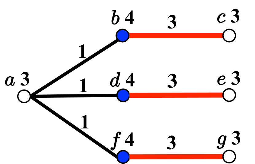
(a) Time-slot 0

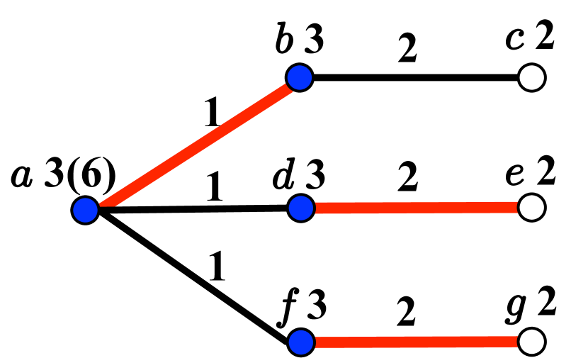
(b) Time-slot 1

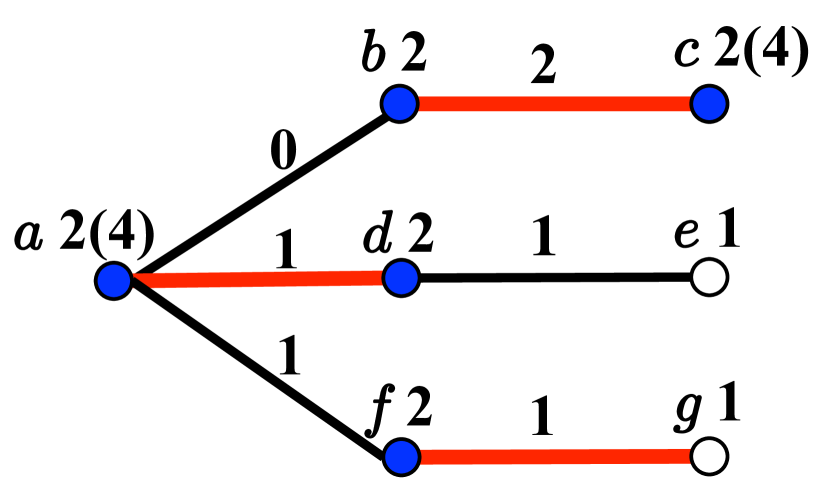
(c) Time-slot 2

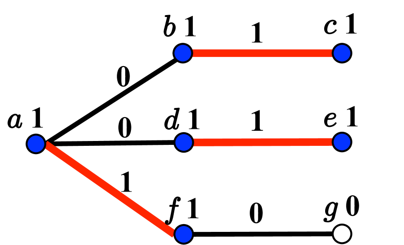
(d) Time-slot 3

Figure 1: An illustration of the operations of NSB in four time-slots. The network setting is presented in Fig. 1(a), where there are seven nodes $\{a,b,\dots,g\}$. In each subfigure, the number above each link denotes the number of packets waiting to be transmitted over that link at the beginning of each time-slot. For simplicity, we assume no future packet arrivals in this example. The node degree (i.e., the sum of queue lengths over all the links touching the node) and the node weight (in the parenthese) are both labeled after the node name; however, the node weight is not labeled if it is equal to the node degree. The heavy nodes are highlighted in blue. Take Fig. 1(b) for example: the heavy nodes are $a$, $b$, $d$, and $d$; node $a$ has a degree of 3 and has a weight of 6; node $b$ has a degree and a weight both equal to 3. Note that although both nodes $a$ and $b$ are heavy nodes in time-slot 1, the weight of $a$ equals twice the node degree because it was not scheduled in time-slot 1 (i.e., $U_{a}(2)=0$). The thick red lines denote the links activated in each time-slot.

(a) Time-slot 0

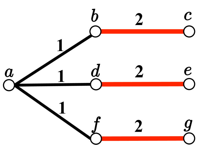
(b) Time-slot 1

(c) Time-slot 2

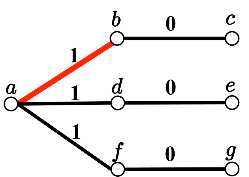
(d) Time-slot 3

Figure 2: An illustration of the operations of MWM in four time-slots. The labels are similar to that in Fig. 1. The node degree and the node weight are not labeled because they are irrelevant under MWM.

Then, in time-slot $k$, we assign a weight to node $i$ as

$$w_{i}(k)\triangleq\begin{cases}Q_{i}(k)(2-U_{i}(k))&\text{if $i\in\mathcal{H}(k)$};\\ Q_{i}(k)&\text{otherwise}.\end{cases}$$ (8)

The NSB algorithm finds an MVM [27] based on the assigned node weight $w_{i}(k)$’s in each time-slot. Note that links with a zero queue length will not be considered when MVM is computed. According to Eq. (8), the nodes are divided into two groups: the heavy nodes that were not scheduled in the previous time-slot(s) have a weight twice their workload, and all the other nodes have a weight equal to their workload. Within each group, a node with a larger workload has a larger weight. To help illustrate the operations of the NSB algorithm, we provide its pseudo code in Algorithm 1.

In addition, to help the reader better understand the operations of the NSB algorithm, we also present a simple example in Fig. 1, which demonstrates the system evolution within four time-slots. Note that a certain tie-breaking rule is applied in this example. Using a different tie-breaking rule, different schedules could be selected. For instance, in time-slot 0 we may activate link $(a,b)$ instead of link $(b,c)$ along with links $(d,e)$ and $(f,g)$. However, tie-breaking rules do not affect our analysis. As can be seen from Fig. 1, NSB drains all initial packets by the end of time-slot 3. For comparison, using the same example, in Fig. 2 we also demonstrate the system evolution under the MWM algorithm. Similarly, we observe that after time-slot 3, MWM needs two more time-slots to completely drain all initial packets. In the next subsection, we will use a similar example to show that a link-based algorithm like MWM needs about twice as much time as that of a node-based algorithm like NSB to evacuate all initial packets in the network.

3.2 Evacuation Time Performance

In this subsection, we analyze the evacuation time performance of NSB in the settings without arrivals. The main result is presented in Theorem 1.

Theorem 1.

The NSB algorithm has an approximation ratio no greater than $3/2$ for the evacuation time performance.

Proof.

Recall that for a given network with initial packets waiting to be transmitted, $\mathcal{X}^{\prime}$ denotes the minimum evacuation time, and $T^{\text{NSB}}$ denotes the evacuation time of NSB. We want to show $T^{\text{NSB}}\leq 3/2\cdot\mathcal{X}^{\prime}$. Recall that $\Delta(0)$ denotes the maximum node queue length in time-slot $0$. If $\Delta(0)=1$, this is trivial as $T^{\text{NSB}}=\mathcal{X}^{\prime}=1$. Now, suppose $\Delta(0)\geq 2$. Then, the result follows immediately from 1) Proposition 1 (stated after this proof): under NSB, the maximum node queue length decreases by at least two within each frame, i.e., $T^{\text{NSB}}\leq 3/2\cdot\Delta(0)$, and 2) an obvious fact: it takes at least $\Delta(0)$ time-slots to drain all the packets over the links incident to a node with maximum queue length, i.e., $\Delta(0)\leq\mathcal{X}^{\prime}$. ∎

Next, we state a key proposition (Proposition 1) used for proving Theorem 1.

Proposition 1.

Consider any frame. Suppose the maximum node queue length is no smaller than two at the beginning of a frame. Under the NSB algorithm, the maximum node queue length decreases by at least two by the end of the frame.

We provide the detailed proof of Proposition 1 in Section 7.1 and give a sketch of the proof below. Note that in any time-slot, the network together with the present packets can be represented as a loopless multigraph, where each multi-edge corresponds to a packet waiting to be transmitted over the link connecting the end nodes of the multi-edge. We use $G(k)$ to denote the multigraph at the beginning of time-slot $k$, and use $M(k)$ to denote the matching found by the NSB algorithm in time-slot $k$. Hence, the degree of node $i$ in $G(k)$ is equivalent to the node queue length $Q_{i}(k)$, and the maximum node degree of $G(k)$ is equal to $\Delta(k)$. Now, consider any frame $k^{\prime}$ consisting of three consecutive time-slots $\{p,p+1,p+2\}$, where $p=3k^{\prime}$. Suppose that the maximum node queue length is no smaller than two at the beginning of frame $k^{\prime}$, i.e., $\Delta(p)\geq 2$ at the beginning of time-slot $p$. Then, we want to show that under the NSB algorithm, the maximum degree will be at most $\Delta(p)-2$ at the end of time-slot $p+2$. We proceed the proof in two steps: 1) we first show that the maximum degree will decrease by at least one in the first two time-slots $p$ and $p+1$ (i.e., the maximum degree will be at most $\Delta(p)-1$ at the end of time-slot $p+1$), and then, 2) show that if the maximum degree decreases by exactly one in the first two time-slots (i.e., the maximum degree is $\Delta(p)-1$ at the end of time-slot $p+1$), then the maximum degree must decrease by one in time-slot $p+2$, and becomes $\Delta(p)-2$ at the end of time-slot $p+2$.

Remark: The key intuition that the NSB algorithm can provide provable evacuation time performance is that all the critical nodes are ensured to be scheduled at least twice within each frame (Proposition 1). This comes from the following properties of NSB: 1) it results in the desired priority or ranking of the nodes by assigning the node weights according to Eq. (8); 2) it finds an MVM based on the assigned node weights, and if a critical node was not scheduled in the first time-slot of the frame, then in the second time-slot of the frame, MVM guarantees to match all such critical nodes (Lemma 1); 3) similarly, if a critical node was not scheduled in both of the first two time-slots of the frame, then MVM guarantees to match all such critical nodes in the third time-slot of the frame.

In addition, we use an example to illustrate why a link-based algorithm like MWM could result in a bad evacuation time performance. Consider the network topology presented in Fig. 3. Since MWM aims to maximize the total weight summed over all scheduled links in each time-slot, it will choose the matching consisting of all the edges with $N$ packets. This pattern repeats until all links have one packet (after $N-1$ time-slots). Then, it takes additional $N$ or $N+1$ time-slots to drain all the remaining packets, depending on the tie-breaking rule. This results in inefficient schedules that consist of one link only about half the time, and thus, requires a total of $2N-1$ or $2N$ time-slots. Another link-based algorithm GMM performs similarly. On the other hand, as we will show in Section 3.4, NSB is evacuation-time-optimal in this example and needs only $\Delta=N+1$ time-slots since the graph is bipartite. The system evolution under NSB and MWM for a special case of $N=3$ can be found in Figs. 1 and 2, respectively.

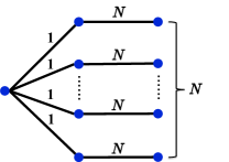
Figure 3: A network with $2N+1$ nodes, where $N$ is a positive integer. The number above each link denotes the number of initial packets waiting to be transmitted over that link.

3.3 Throughput Performance

Next, we analyze the throughput performance of NSB in the settings with arrivals. The main result is presented in Theorem 2.

Theorem 2.

The NSB algorithm has an efficiency ratio no smaller than $2/3$ for the throughput performance.

We will employ fluid limit techniques [28, 29, 26] to prove Theorem 2. Fluid limit techniques are useful for two main reasons: (i) it removes irrelevant randomness in the original stochastic system such that the considered system becomes deterministic and thus, the analysis can be simplified; (ii) the algorithm exhibits some special properties in the fluid limit (e.g., Lemma 3), which do not exist in the original stochastic system.

Before proving Theorem 2, we construct the fluid model and state some definitions and a lemma that will be used in the proof. First, we extend the process $Y=A,Q,D,H$ to continuous time $t\geq 0$ by setting $Y(t)=Y(\lfloor t\rfloor)$. Hence, $A(t)$, $Q(t)$, $D(t)$, and $H(t)$ are right continuous with left limits. Then, using the techniques of [29], we can show that for almost all sample paths and for all positive sequences ${x_{r}}\rightarrow\infty$, there exists a subsequence ${x_{r_{j}}}$ with ${x_{r_{j}}}\rightarrow\infty$ as $j\rightarrow\infty$ such that the following convergence holds uniformly over compact (u.o.c.) intervals of time $t$:

$$\frac{A_{i}({x_{r_{j}}}t)}{{x_{r_{j}}}}\rightarrow\lambda_{i}t,~{}\text{for all}~{}i\in V,$$ (9)

$$\frac{Q_{i}({x_{r_{j}}}t)}{{x_{r_{j}}}}\rightarrow q_{i}(t),~{}\text{for all}~{}i\in V,$$ (10)

$$\frac{D_{i}({x_{r_{j}}}t)}{{x_{r_{j}}}}\rightarrow d_{i}(t),~{}\text{for all}~{}i\in V,$$ (11)

$$\frac{H_{M}({x_{r_{j}}}t)}{{x_{r_{j}}}}\rightarrow h_{M}(t),~{}\text{for all}~{}M\in\mathcal{M}.$$ (12)

Since the proof of the above convergence is standard, we provide the proof in the appendix for completeness.

Next, we present the fluid model equations as follows:

$$q_{i}(t)=q_{i}(0)+\lambda_{i}t-d_{i}(t),~{}\text{for all}~{}i\in V,$$ (13)

$${\textstyle\frac{d}{dt}}d_{i}(t)=\sum_{M\in\mathcal{M}}\sum_{l\in L(i)}M_{l}\cdot{\textstyle\frac{d}{dt}}h_{M}(t),~{}\text{for all}~{}i\in V,$$ (14)

$$\sum_{M\in\mathcal{M}}h_{M}(t)=t.$$ (15)

Any such limit $(q,d,h)$ is called a fluid limit. Note that $q_{i}(\cdot),d_{i}(\cdot)$ and $h_{i}(\cdot)$ are absolutely continuous functions and are differentiable at almost all times $t\geq 0$ (called regular times). Taking the derivative of both sides of (13) and substituting (14) into it, we obtain

$$\begin{split}{\textstyle\frac{d}{dt}}q_{i}(t)&=\lambda_{i}-{\textstyle\frac{d}{dt}}d_{i}(t)\\ &=\lambda_{i}-\sum_{M\in\mathcal{M}}\sum_{l\in L(i)}M_{l}\cdot{\textstyle\frac{d}{dt}}h_{M}(t).\end{split}$$ (16)

Borrowing the results of [29], we give the definition of weak stability and state Lemma 2, which establishes the connection between rate stability of the original system and weak stability of the fluid model.

Definition 2.

The fluid model of a network is weakly stable if for every fluid model solution $(q,d,h)$ with $q(0)=0$, one has $q(t)=0$ for all regular times $t\geq 0$.

Lemma 2 (Theorem 3 of [29]).

A network is rate stable if the associated fluid model is weakly stable.

We are now ready to prove Theorem 2.

Proof of Theorem 2.

We want to show that given any arrival rate vector $\lambda$ strictly inside $2/3\cdot\Lambda^{*}$, the system is rate stable under the NSB algorithm. Note that $\lambda$ is also strictly inside $2/3\cdot\Psi$ (i.e., $\lambda_{i}<2/3$ for all $i\in V$) since $\Lambda^{*}\subseteq\Psi$. We define $\epsilon\triangleq\min_{i\in V}(2/3-\lambda_{i})$. Clearly, we must have $\epsilon>0$.

To show rate stability of the original system, it suffices to show weak stability of the fluid model due to Lemma 2. We start by defining the following Lyapunov function:

$$V(q(t))=\max_{i\in V}q_{i}(t).$$ (17)

For any regular time $t\geq 0$, we define the drift of $V(q(t))$ as its derivative, denoted by ${\textstyle\frac{d}{dt}}V(q(t))$. Since $V(q(t))$ is a non-negative function, given $q(0)=0$, in order to show $V(q(t))=0$ and thus $q(t)=0$ for all regular times $t\geq 0$, it suffices to show that if $V(q(t))>0$ for $t>0$, then $V(q(t))$ has a negative drift. This is due to a simple result in Lemma 1 of [29]. Therefore, we want to show that for all regular times $t>0$, if $V(q(t))>0$, then ${\textstyle\frac{d}{dt}}V(q(t))\leq-\epsilon$.

We first fix time $t$ and let $q_{\max}(t)=V(q(t))=\max_{i\in V}q_{i}(t)$. Define the set of critical nodes in the fluid limits at time $t$ as

$$\mathcal{C}\triangleq\{i\in V~{}|~{}q_{i}(t)=q_{\max}(t)\}.$$ (18)

Also, let $\hat{q}_{\max}(t)$ be the largest queue length in the fluid limits among the remaining nodes, i.e., $\hat{q}_{\max}(t)=\max_{i\in V\backslash\mathcal{C}}q_{i}(t)$. Since the number of nodes is finite, we have $\hat{q}_{\max}(t)<q_{\max}(t)$. Choose $\beta$ small enough such that $\hat{q}_{\max}(t)<q_{\max}(t)-3\beta$ and $\beta<q_{\max}(t)/(2n-1)$. Our choice of $\beta$ implies the following:

$$q_{\max}(t)-\beta>\frac{n-1}{n}(q_{\max}(t)+\beta).$$ (19)

Recall that $q(t)$ is absolutely continuous. Hence, there exists a small $\delta$ such that the queue lengths in the fluid limits satisfy the following condition for all times $\tau\in(t,t+\delta)$ and for all nodes $i\in V$:

$$q_{i}(\tau)\in\left(q_{i}(t)-\beta/2,q_{i}(t)+\beta/2\right).$$ (20)

This further implies that the following conditions hold:

(C1) $q_{i}(\tau)\in(q_{\max}(t)-\beta/2,q_{\max}(t)+\beta/2)$ for all $i\in\mathcal{C}$;

(C2) $q_{i}(\tau)<q_{\max}(t)-5\beta/2$ for all $i\notin\mathcal{C}$,

where (C2) is from Eq. (20) and $q_{i}(t)\leq\hat{q}_{\max}(t)<q_{\max}(t)-3\beta$ for all $i\notin\mathcal{C}$.

Let ${x_{r_{j}}}$ be a positive subsequence for which the convergence to the fluid limit holds. Consider a large enough $j$ such that $\left\lvert Q_{i}({x_{r_{j}}}\tau)/{x_{r_{j}}}-q_{i}(\tau)\right\rvert<\beta/2$ for all $\tau\in(t,t+\delta)$. Considering the interval $(t,t+\delta)$ around time $t$, we define a set of consecutive time-slots in the original system as $T\triangleq\{\lceil{x_{r_{j}}}t\rceil,\lceil{x_{r_{j}}}t\rceil+1,\dots,\lfloor{x_{r_{j}}}(t+\delta)\rfloor\}$, which corresponds to the scaled time interval $(t,t+\delta)$ in the fluid limits.

Lemma 3 states that NSB, all the critical nodes at scaled time $t$ in the fluid limits will be scheduled at least twice within each frame of interval $T$.

Lemma 3.

Under the NSB algorithm, all the nodes in $\mathcal{C}$ will be scheduled at least twice within each frame of interval $T$.

We provide the proof of Lemma 3 in Section 7.2. For now, we assume that Lemma 3 holds. Note that interval $T$ contains at least $(\lfloor{x_{r_{j}}}(t+\delta)\rfloor-\lceil{x_{r_{j}}}t\rceil-3)/3$ complete frames. Then, from Lemma 3, we have that for all $i\in\mathcal{C}$,

$$\begin{split}&\sum_{M\in\mathcal{M}}\sum_{l\in L(i)}M_{l}\cdot(H_{M}({x_{r_{j}}}(t+\delta))-H_{M}({x_{r_{j}}}t))\\ &\geq 2/3\cdot(\lfloor{x_{r_{j}}}(t+\delta)\rfloor-\lceil{x_{r_{j}}}t\rceil-3),\end{split}$$ (21)

and therefore, we have

$$\begin{split}&\sum_{M\in\mathcal{M}}\sum_{l\in L(i)}M_{l}\cdot{\textstyle\frac{d}{dt}}h_{M}(t)\\ &=\lim_{\delta\rightarrow 0}\sum_{M\in\mathcal{M}}\sum_{l\in L(i)}M_{l}\cdot\frac{h_{M}(t+\delta)-h_{M}(t)}{\delta}\\ &\stackrel{{\scriptstyle(a)}}{{=}}\lim_{\delta\rightarrow 0}\lim_{j\rightarrow\infty}\sum_{M\in\mathcal{M}}\sum_{l\in L(i)}\frac{M_{l}\cdot(H_{M}({x_{r_{j}}}(t+\delta))-H_{M}({x_{r_{j}}}t))}{{x_{r_{j}}}\delta}\\ &\stackrel{{\scriptstyle(b)}}{{\geq}}\lim_{\delta\rightarrow 0}\lim_{j\rightarrow\infty}\frac{2/3\cdot(\lfloor{x_{r_{j}}}(t+\delta)\rfloor-\lceil{x_{r_{j}}}t\rceil-3)}{{x_{r_{j}}}\delta}\\ &=2/3,\end{split}$$ (22)

where $(a)$ is from the convergence in Eq. (12) and $(b)$ is from Eq. (21). Then, it follows from Eq. (16) that for all $i\in\mathcal{C}$, we have ${\textstyle\frac{d}{dt}}q_{i}(t)\leq\lambda_{i}-2/3\leq-\epsilon$.

Also, from conditions (C1) and (C2), every node $i\notin\mathcal{C}$ has a queue length strictly smaller than that of a critical node in $\mathcal{C}$ for the entire duration $(t,t+\delta)$. Thus, we have ${\textstyle\frac{d}{dt}}V(q(t))\leq-\epsilon$, which implies that the fluid model is weakly stable. Then, we complete the proof by applying Lemma 2. ∎

Remark: The key intuition that the NSB algorithm can provide provable throughput performance is that all the critical nodes in the fluid limit are ensured to be scheduled at least twice within each frame of interval $T$ (Lemma 3). Similar to the provable evacuation time performance, this comes from the desired weight assignment (Eq. (8)) and an important property of MVM (Lemma 1).

As we mentioned earlier, the proof of Lemma 3 is provided in Section 7.2. However, we want to emphasize that the proof relies on a novel application of graph-factor theory, which is stated in Lemma 4. Lemma 4 is of critical importance in proving the guaranteed throughput performance of the NSB algorithm in general graphs. Moreover, it will play a key role in establishing both throughput optimality and evacuation time optimality for NSB in bipartite graphs (see Section 3.4).

Next, we give some additional notations that are needed to state Lemma 4. By slightly abusing the notations, we also use $G=(V,E)$ to denote a multigraph, which is possibly not loopless. Let $d_{G}(v)$ be the degree of node $v$ in $G$, where a loop associated with node $v$ counts 2 towards the degree of $v$. Also, let $G_{Z}$ denote the subgraph of $G$ induced by a subset of nodes $Z\subseteq V$.

Lemma 4.

Let $G=(V,E)$ be a multigraph with maximum degree $\Delta$. Consider a subset of nodes $Z\subseteq V$. Suppose that the following conditions are satisfied: (i) all the nodes of $Z$ are heavy nodes, i.e., $Z\subseteq\{v\in V~{}|~{}d_{G}(v)\geq(n-1)/n\cdot\Delta\}$, and (ii) $G_{Z}$ is bipartite. Then, there exists a matching of $G$ that matches every node of $Z$.

Proof.

We first introduce some additional notations. Let $g=[g_{v}:v\in V]$ and $f=[f_{v}:v\in V]$ be vectors of positive integers satisfying

$$0\leq g_{v}\leq f_{v}\leq d_{G}(v),~{}\text{for all}~{}v\in V.$$ (23)

A $(g,f)$-factor is a subgraph $F$ of $G$ with

$$g_{v}\leq d_{F}(v)\leq f_{v},~{}\text{for all}~{}v\in V.$$ (24)

Note that if vectors $g$, $f$ satisfy $g_{v},f_{v}\in\{0,1\}$ for all $v\in V$, then the edges of a $(g,f)$-factor form a matching of $G$. Let $G_{g=f}$ denote the subgraph of $G$ induced by nodes $v$ for which $g_{v}=f_{v}$, and let $[x]^{+}\triangleq\max\{x,0\}$. We restate a result of [30] in Lemma 5, which will be used in the proof.

Lemma 5 (Theorem 1.3 of [30], Property I).

Let multigraph $G$ and vectors $g$, $f$ be given. Suppose that $G_{g=f}$ is bipartite. Then, $G$ has a $(g,f)$-factor if and only if for all node subsets $S\subseteq V$,

$$\sum_{v\in S}f_{v}\geq\sum_{v\notin S}[g_{v}-d_{G-S}(v)]^{+}.$$ (25)

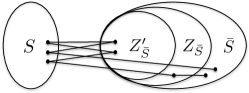
Figure 4: An illustration for the relationship of the sets in the proof of Lemma 4.

We are now ready to prove Lemma 4. Suppose that (i) all the nodes of $Z$ are heavy nodes and (ii) $G_{Z}$ is bipartite. We construct vectors $g$, $f$ by setting $g_{v}=f_{v}=1$ for node $v\in Z$ and $g_{v}=0$, $f_{v}=1$ otherwise. With our constructed vectors $g$ and $f$, not only a $(g,f)$-factor forms a matching of graph $G$, but this matching also matches every node of $Z$. Therefore, it suffices to show that $G$ has a $(g,f)$-factor.

Next, we apply Lemma 5 to show that $G$ has a $(g,f)$-factor. Note that $G_{g=f}=G_{Z}$ and $G_{Z}$ is bipartite. Then, it remains to show that Eq. (25) is satisfied for any subset of nodes $S\subseteq V$. Let $\bar{S}=V\backslash S$ be the complementary set of $S$. Let $Z_{\bar{S}}=Z\cap\bar{S}$, and let $Z_{\bar{S}}^{\prime}=\{v\in Z_{\bar{S}}~{}|~{}$ all the neighboring nodes of $v$ are in $S\}$. The relationship of these sets is illustrated in Fig. 4. Clearly, we have $\sum_{v\in S}f_{v}=\lvert S\rvert$ as $f_{v}=1$ for all $v\in V$. Also, a little thought gives $\sum_{v\notin S}[g_{v}-d_{G-S}(v)]^{+}=\lvert Z_{\bar{S}}^{\prime}\rvert$. This is because any node $v\notin S$ must belong to one of the following three cases:

1. If $v\notin Z$, then $g_{v}=0$, and thus, $[g_{v}-d_{G-S}(v)]^{+}=0$;

2. If $v\in Z_{\bar{S}}\backslash Z_{\bar{S}}^{\prime}$, then $g_{v}=1$ and $d_{G-S}(v)\geq 1$, which implies $[g_{v}-d_{G-S}(v)]^{+}=0$;

3. If $v\in Z_{\bar{S}}^{\prime}$, then $g_{v}=1$ and $d_{G-S}(v)=0$, which implies $[g_{v}-d_{G-S}(v)]^{+}=1$.

Hence, in order to show Eq. (25), it remains to show $\lvert S\rvert\geq\lvert Z_{\bar{S}}^{\prime}\rvert$. We prove it by contradiction. Suppose $\lvert S\rvert<\lvert Z_{\bar{S}}^{\prime}\rvert$. Since $S$ and $Z_{\bar{S}}^{\prime}$ are disjoint, we have $\lvert S\rvert+\lvert Z_{\bar{S}}^{\prime}\rvert\leq n$, and thus, $\lvert S\rvert<n$. We let $d_{G}(Z)=\sum_{i\in Z}d_{G}(i)$ denote the total degree of a subset of nodes $Z\subseteq V$ in $G$. Then, we state three obvious facts:

(F1) $d_{G}(Z_{\bar{S}}^{\prime})\geq(n-1)/n\cdot\Delta\lvert Z_{\bar{S}}^{\prime}\rvert$;

(F2) $d_{G}(S)\leq\Delta\lvert S\rvert$;

(F3) $d_{G}(Z_{\bar{S}}^{\prime})\leq d_{G}(S)$.

Note that (F1) is from the fact that every node of $Z$ has a degree no smaller than $(n-1)/n\cdot\Delta$, (F2) is trivial, and (F3) is from the definition of $Z_{\bar{S}}^{\prime}$ that all of its neighboring nodes belong to $S$. Then, by combining the above facts, we obtain

$$\frac{n-1}{n}\leq\frac{\lvert S\rvert}{\lvert Z_{\bar{S}}^{\prime}\rvert}.$$ (26)

This further implies $\lvert Z_{\bar{S}}^{\prime}\rvert-\lvert S\rvert\leq\lvert S\rvert/(n-1)\leq 1$, as $\lvert S\rvert<n$. Hence, we must have $\lvert Z_{\bar{S}}^{\prime}\rvert=\lvert S\rvert+1$, because $\lvert S\rvert<\lvert Z_{\bar{S}}^{\prime}\rvert$. Substituting this back into Eq. (26) gives $(n-1)/n\leq\lvert S\rvert/(\lvert S\rvert+1)$. This implies $\lvert S\rvert\geq n-1$, and thus $\lvert S\rvert+\lvert Z_{\bar{S}}^{\prime}\rvert\geq 2n-1$, which contradicts the fact that $\lvert S\rvert+\lvert Z_{\bar{S}}^{\prime}\rvert\leq n$. (We assume $n>1$ to avoid trivial discussions.)

Therefore, we have $\lvert S\rvert\geq\lvert Z_{\bar{S}}^{\prime}\rvert$, and thus, Eq. (25) is satisfied. Then, Lemma 5 implies that graph $G$ has a $(g,f)$-factor, which forms a matching of graph $G$ that matches every node of $Z$. This completes the proof. ∎

3.4 Optimality in Bipartite Graphs

As we have explained in the introduction, the minimum evacuation time is lower bounded by the largest workload at the nodes and the odd-size cycles. Hence, both the nodes and the odd-size cycles could be bottlenecks. Ideally, it would be best to consider the workload of both the nodes and the odd-size cycles when making scheduling decisions. However, this may render the algorithm very complex because it is much more difficult to explicitly consider all the odd-size cycles in a graph. Hence, we have focused on designing the node-based algorithms (such as the NSB algorithm) that do not explicitly handle the odd-size cycles. Without considering all the bottlenecks, these algorithms may not be able to achieve the best achievable performance in general. However, the theoretical results of Theorems 1 and 2 are quite remarkable in the sense that even without considering the odd-size cycles (which could also be bottlenecks), the NSB algorithm can guarantee an approximation ratio no greater than $3/2$ for the evacuation time and an efficiency ratio no smaller than $2/3$ for the throughput. We believe that NSB will perform better if odd-size cycles do not form bottlenecks. This is also observed from our simulation results in Section 5.

In this subsection, we will show that NSB is both throughput-optimal and evacuation-time-optimal in bipartite graphs, where there are no odd-size cycles. This result is stated in Theorem 3, whose proof needs to apply Lemmas 4 and 1 and follows a similar line of analysis to that of Theorems 1 and 2 for general graphs. The detailed proof is provided in the appendix for completeness.

Theorem 3.

The NSB algorithm is both throughput-optimal and evacuation-time-optimal in bipartite graphs.

Remark: The NSB algorithm has a complexity of $O(m\sqrt{n}\log n)$, as the complexity of finding an MVM is $O(m\sqrt{n}\log n)$ [27]. One important question is whether we can develop lower-complexity algorithms that provide the same performance guarantees. We answer this question in the next section.

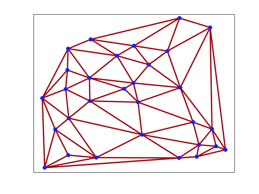
(a) Triangular Mesh

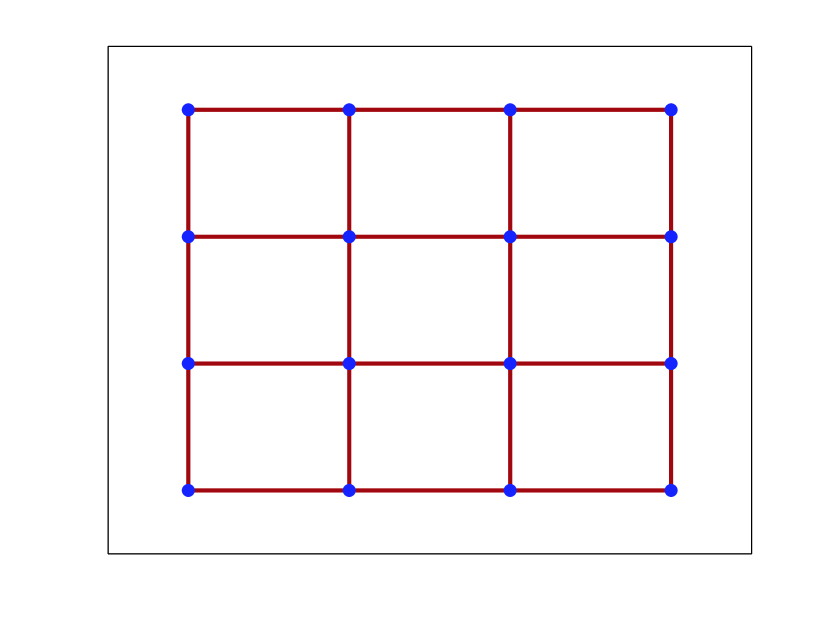
(b) 4$\times$4 grid

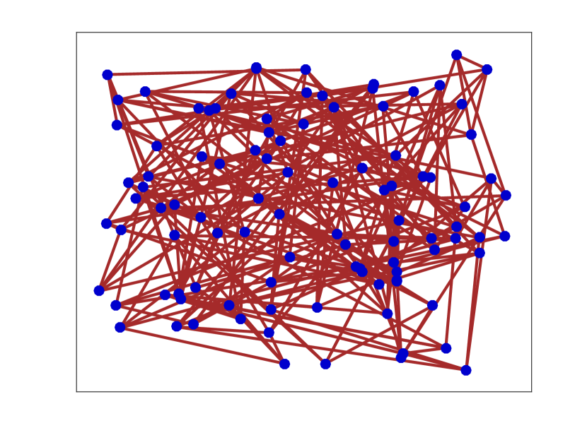
(c) Random topology

Figure 5: Simulation Topologies.

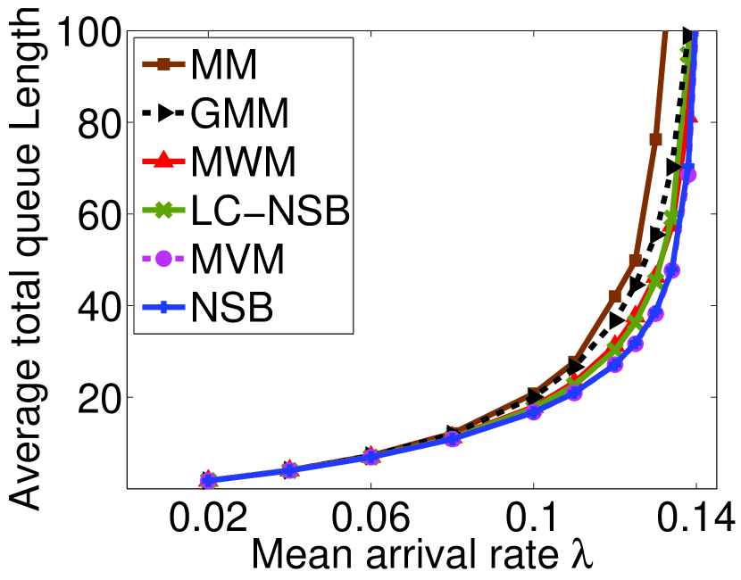
(a) Triangular Mesh

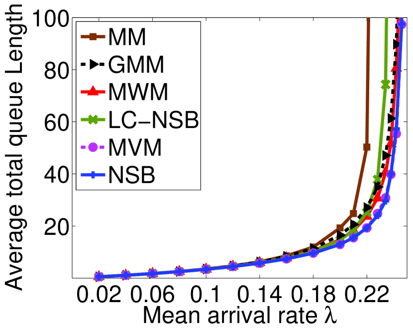
(b) 4$\times$4 grid

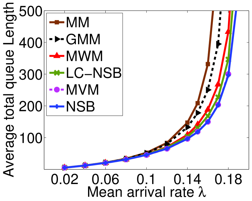
(c) Random topology

Figure 6: Simulation results for Poisson arrivals.

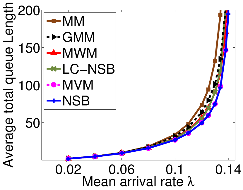
(a) Triangular Mesh

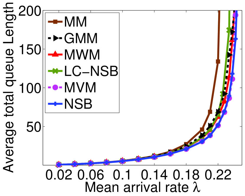
(b) 4$\times$4 grid

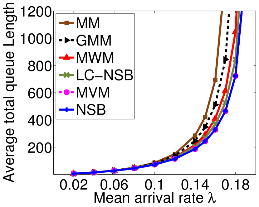
(c) Random topology

Figure 7: Simulation results for file arrivals, where the file arrival probability is $p=0.1$ and the file size follows Poisson distribution with mean $\lambda/p$.

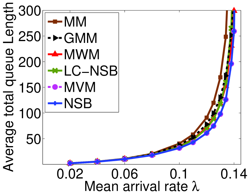
(a) Triangular Mesh

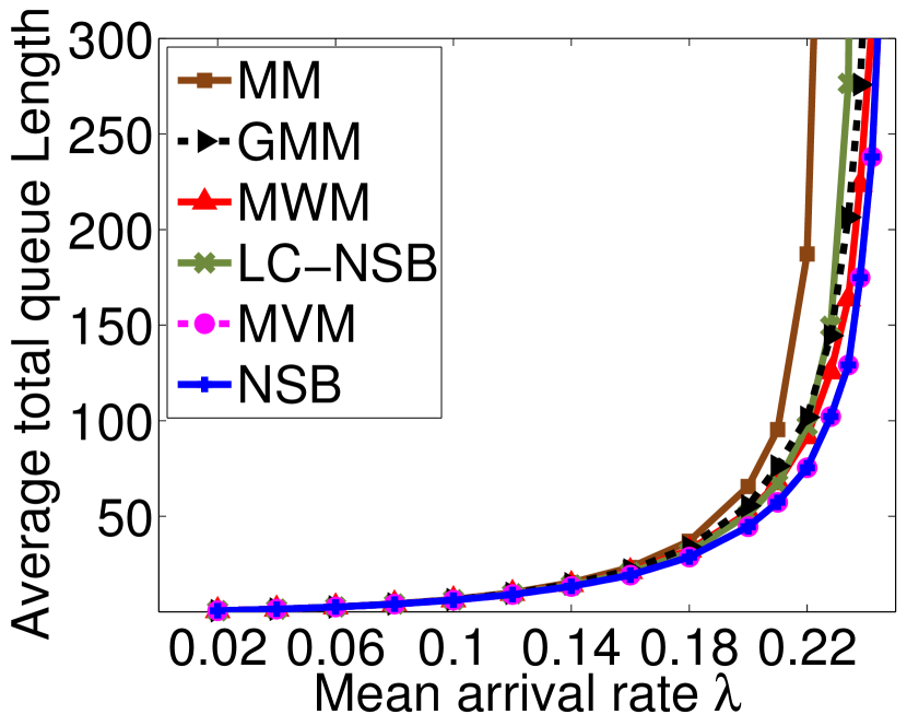
(b) 4$\times$4 grid

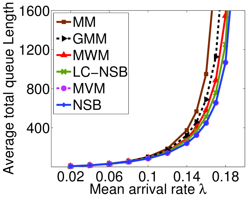
(c) Random topology

Figure 8: Simulation results for Zipf arrivals with a support of $[0,1,\dots,999]$.

4 A Lower-Complexity NSB Algorithm

Through the analysis for the NSB algorithm, we obtain the following important insights: In order to achieve the same performance guarantees as NSB, what really matters is the priority or the ranking of the nodes, rather than the exact weight of the nodes. This insight comes from the following: Note that under the NSB algorithm, the weight of each node is only used in the MVM component (line 6 of Algorithm 1). In the performance analysis of NSB (i.e., Theorems 1, 2, and 3), the only property of MVM we use is Lemma 1, which is concerned about the $s$ heaviest nodes (i.e., the $s$ highest ranking nodes) rather than about the exact weight of the nodes. Hence, if we assign the node weights in a way such that, the weights are bounded integers and the nodes still have the desired priority or ranking as in the NSB algorithm, then we can develop a new algorithm with a lower complexity. Thanks to the results of [31, 32], an $O(m\sqrt{n})$-complexity implementation of MVM can be derived if the maximum node weight is a bounded integer independent of $n$ and $m$.

Next, we propose such an algorithm, called the Lower-Complexity NSB (LC-NSB). Similarly as in NSB, we consider frames each consisting of three consecutive time-slots. Recall that $U_{i}(k)$ indicates whether node $i$ was matched in the previous time-slot (or in both of the previous two time-slots), as defined in Eq. (7). Also, recall that $\mathcal{C}(k)$ and $\mathcal{H}(k)$ denote the set of critical nodes and the set of heavy nodes in time-slot $k$, respectively. In time-slot $k$, we assign a weight to node $i$ as

$$w_{i}(k)\triangleq\begin{cases}5-2U_{i}(k)&\text{if $i\in\mathcal{C}(k)$};\\ 4-2U_{i}(k)&\text{if $i\in\mathcal{H}(k)\backslash\mathcal{C}(k)$};\\ 1&\text{otherwise}.\end{cases}$$ (27)

Then, the LC-NSB algorithm finds an MVM based on the assigned node weight $w_{i}(k)$’s in every time-slot. Note that LC-NSB has a very similar way of assigning the node weights as NSB. However, the key difference is that we now divide all the nodes into five priority groups by assigning the node weights only based on whether it is a heavy (or critical) node and whether it was scheduled in the previous time-slot(s), while in the NSB algorithm, the actual workload is used in the weight assignments. This slight yet crucial change leads to a lower-complexity algorithm with the same performance guarantees. Note that in Eq. (27), we give a higher priority to the critical nodes in order to guarantee the evacuation time performance. The proof follows a similar line of analysis to that for the NSB algorithm and is provided in the appendix for completeness.

Theorem 4.

The LC-NSB algorithm has an approximation ratio no greater than $3/2$ for the evacuation time and has an efficiency ratio no smaller than $2/3$ for the throughput. Moreover, the LC-NSB algorithm is both throughput-optimal and evacuation-time-optimal in bipartite graphs.

Remark: Although the LC-NSB algorithm can provide the same performance guarantees as NSB, we would expect that LC-NSB may have (slightly) worse empirical performance compared to NSB, since NSB has a more fine-grained priority differentiation among all the nodes. We indeed make such observations in our simulation results in Section 5. In order to improve the empirical performance, we can introduce more priority groups for the non-heavy nodes under LC-NSB rather than all being in the same priority group (of weight 1 as in Eq. (27)). As long as the number of priority groups is a bounded integer independent of $n$ and $m$, the complexity remains $O(m\sqrt{n})$.

5 Numerical Results

In this section, we conduct numerical experiments to elucidate our theoretical results. We also compare the empirical performance of our proposed NSB and LC-NSB algorithms with several most relevant algorithms as listed in Table I.

5.1 Throughput Performance

To evaluate the throughput performance, we run the simulations on three different network topologies as shown in Fig. 5. We first focus on a randomly generated triangular mesh topology with 30 nodes and 79 links as shown in Fig. 5(a). The simulations are implemented using C++. We assume that the arrivals are i.i.d. over all the links with unit capacity. The mean arrival rate of each link is $\lambda$, and the instantaneous arrivals to each link follow a Poisson distribution in each time-slot. In Fig. 6(a), we plot the average total queue length in the system against the arrival rate $\lambda$. We consider several values of $\lambda$ as indicated in Fig. 6(a). For each value of $\lambda$, the average total queue length is an average of 10 independent simulations. Each individual simulation runs for a period of $10^{5}$ time-slots. We compute the average total queue length by excluding the first $5\times 10^{4}$ time-slots in order to remove the impact of the initial transient state. Note that this network topology contains odd-size cycles. Hence, our proposed NSB and LC-NSB only guarantee to achieve $2/3$ of the optimal throughput. However, the simulation results in Fig. 6(a) show that NSB and LC-NSB algorithms both empirically achieve the optimal throughput performance. This is because the odd-size cycles (i.e., all the triangles in this case) do not form the bottlenecks in this setting. For example, a triangle requires $\lambda\leq 1/3$ because at most one of its three links can be scheduled in each time-slot. However, in Fig. 5(a) there exists a node touched by seven links, which requires $\lambda\leq 1/7$. As the load $\lambda$ increases, such a node will become congested sooner than any triangle and thus forms a scheduling bottleneck.

We also conduct simulations for a 4$\times$4 grid topology with 16 nodes and 24 links (Fig. 5(b)) and a randomly generated dense topology with 100 nodes and 248 links (Fig. 5(c)). All the other simulation settings are the same as that for the triangular mesh topology. The simulation results are presented in Fig. 6. The observations we make are similar to that for the triangular mesh topology, except that in the grid topology, LC-NSB has higher delays when the mean arrival rate approaches the boundary of the optimal throughput region. This is due to the following two reasons: 1) Under LC-NSB, all the non-heavy nodes are in the same priority group of weight 1, so a non-heavy node with a large workload would have a similar chance of getting scheduled as a non-heavy node with a small workload; 2) In the grid topology, the bottleneck nodes (i.e., the four nodes in the center) are all adjacent. Note that in most cases, at least one of the bottleneck nodes is the critical node and will have the highest priority. If another bottleneck node is adjacent to the critical node but is not a heavy node, this bottleneck node will get a lower chance of being scheduled, since the critical node could be matched with other node. This inefficiency does not occur under NSB, since the node weights of the non-heavy nodes are their workload and are more fine-grained. Hence, a non-heavy node with a large workload will have a higher priority than a non-heavy node with a small workload.

In order to evaluate the throughput performance under different arrival patterns, we also run simulations for file arrivals. Specifically, the arrivals have the following pattern: in each time-slot, there is a file arrival with probability $p$, and no file arrival otherwise; the file size follows Poisson distribution with mean $\lambda/p$. The simulation results for $p=0.1$ are presented in Fig. 7. Similar observations to that for Poisson arrivals can be made, except that all the algorithms have larger delays due to a more bursty arrival pattern. In addition, we also consider more realistic arrival patterns where the arrivals in each time-slot follow the Zipf law, which is commonly used to model the Internet traffic [33]. We assume a support of $[0,1,\dots,999]$ for the Zipf distribution. The power exponent of the Zipf distribution is determined based on the mean arrival rate $\lambda$. The simulation results are presented in Fig. 8. The overall observations are again similar to that for the previous arrival patterns.

Finally, it is remarkable that in all simulation settings we consider, our proposed node-based algorithm NSB empirically achieves the best delay performance. When the traffic load is high, NSB even results in a significant reduction (10%-30%) in the average delay performance compared to the link-based algorithms such as MWM (e.g., in Fig. 8(c) for a random topology with Zipf arrivals, the delay reduction is about 30% when $\lambda=0.18$). Although NSB ties with another node-based algorithm MVM for the empirical delay performance, as we discussed in the introduction, the throughput performance of MVM is not well understood yet.

5.2 Evacuation Time Performance

In this subsection, we evaluate the evacuation time performance of our proposed algorithms. As we discussed in the introduction, the minimum evacuation time problem is equivalent to the classic multigraph edge coloring problem, for which there are common benchmarks. Therefore, we run simulations for six DIMACS benchmark instances [34] for the graph coloring problem. In addition, we also run simulations for three regular multigraphs, three random multigraphs, and one special graph (Fig. 3 with $N=100$).

The evacuation time performance for each of the considered algorithms under each graph is presented in Table III. The simulation results show that all the algorithms have very similar evacuation time performance for the considered benchmark graphs and regular multigraphs, although they have different theoretical guarantees. For the special graph in Fig. 3, we can observe that the node-based algorithms exhibit a much better evacuation time performance compared to the link-based algorithms (e.g., MWM and GMM). Specifically, the link-based algorithms require about twice as much time as that of the node-based algorithms to evacuate all initial packets in the network.

6 Conclusion

In this paper, we studied the link scheduling problem for multi-hop wireless networks and focused on designing efficient online algorithms with provably guaranteed throughput and evacuation time performance. We developed two node-based service-balanced algorithms and showed that none of the existing algorithms strike a more balanced performance guarantees than our proposed algorithms in both dimensions of throughput and evacuation time. An important future direction is to consider more general models (which, e.g., allow for multi-hop traffic, general interference models, and time-varying channels). In such scenarios, it becomes much more challenging to provide provably good evacuation time performance.

Graph	MWM	GMM	MVM	NSB	LC-NSB	$\Delta$
dsjc125.1	23	23	23	23	23	23
dsjc125.5	76	75	75	75	75	75
dsjc125.9	140	120	120	120	120	120
dsjc250.1	38	40	38	38	38	38
dsjc250.5	147	153	147	147	147	147
dsjc250.9	234	234	234	234	234	234
regm50.20	20	25	20	20	20	20
regm50.50	50	55	51	51	51	50
regm50.80	80	84	80	80	80	80
rand100.50	366	366	366	366	366	366
rand100.100	813	813	813	813	813	813
rand100.250	2161	2161	2161	2161	2161	2161
Fig. 3	199	199	101	101	101	101

TABLE III: Evacuation time performance for six DIMACS benchmark graphs [34], three regular multigraphs, and one special graph (Fig. 3 with $N=100$). In the table, $\Delta$ denotes the maximum node degree, dsjcX.Y denotes the label of the DIMACS benchmark graphs, regmX.Y denotes a regular mutigraph with X nodes and node degree Y, and randX.Y denotes a random topology in Fig. 5(c) with X nodes and the number of multi-edges at each link being uniformly distributed over the interval [0,Y].

7 Proofs

7.1 Proof of Proposition 1

We first restate a useful result of [35] in Lemma 6, which will be used in the proof of Proposition 1. Throughout the paper, we assume that the multigraph is loopless (i.e., there is no edge connecting a node to itself) unless explicitly mentioned.

Lemma 6 (Theorem 1 of [35]).

Let $G$ be a loopless multigraph with maximum degree $\Delta$. Let $G_{\Delta}$ denote the subgraph of $G$ induced by all the nodes having maximum degree. If $G_{\Delta}$ is bipartite, then there exists a matching over $G$ that matches every node of maximum degree.

Now, we are ready to prove Proposition 1.

Proof of Proposition 1.

First, note that in any time-slot, the network together with the present packets can be represented as a loopless multigraph. Recall that $G(k)$ denotes the multigraph at the beginning of time-slot $k$ and $M(k)$ denotes the matching found by the NSB algorithm in time-slot $k$. Also, recall that the degree of node $i$ in $G(k)$ is equivalent to the node queue length $Q_{i}(k)$, and the maximum node degree of $G(k)$ is equal to $\Delta(k)$. Now, consider any frame $k^{\prime}$ consisting of three consecutive time-slots $\{p,p+1,p+2\}$, where $p=3k^{\prime}$. Suppose that the maximum node queue length is no smaller than two at the beginning of frame $k^{\prime}$, i.e., $\Delta(p)\geq 2$ at the beginning of time-slot $p$. Then, we want to show that under the NSB algorithm, the maximum degree will be at most $\Delta(p)-2$ at the end of time-slot $p+2$. We proceed the proof in two steps: 1) we first show that the maximum degree will decrease by at least one in the first two time-slots $p$ and $p+1$ (i.e., the maximum degree will be at most $\Delta(p)-1$ at the end of time-slot $p+1$), and then, 2) show that if the maximum degree decreases by exactly one in the first two time-slots (i.e., the maximum degree is $\Delta(p)-1$ at the end of time-slot $p+1$), then the maximum degree must decrease by one in time-slot $p+2$, and becomes $\Delta(p)-2$ at the end of time-slot $p+2$.

We start with step 1). It is a trivial case if the maximum degree decreases by one in time-slot $p$. Therefore, suppose the maximum degree does not decrease in time-slot $p$. Then, it suffices to show that all the nodes having maximum degree $\Delta(p)$ in $G(p+1)$ must be scheduled in time-slot $p+1$ under the NSB algorithm. Note that matching $M(k)$ must be a maximal matching over $G(k)$ for every time-slot $k$. Since $M(p)$ is a maximal matching, the nodes having maximum degree must form an independent set over $G(p+1)$ at the beginning of time-slot $p+1$. We prove this by contradiction. Note that if there is only one node having maximum degree at the beginning of time-slot $p+1$, then it is trivial that the subgraph induced by this single node must consist of this node itself only and thus forms an independent set. So we consider the case where there are at least two nodes having maximum degree at the beginning of time-slot $p+1$. Suppose node $i$ and node $j$ are two adjacent nodes having maximum degree $\Delta(p)$ at the beginning of time-slot $p+1$. Then, none of the edges incident to either $i$ or $j$ was in matching $M(p)$. This implies that the edge between $i$ and $j$ can be added to matching $M(p)$ in time-slot $p$, which, however, contradicts the fact that $M(p)$ is a maximal matching. Therefore, the nodes having maximum degree must form an independent set at the beginning of time-slot $p+1$. Clearly, the subgraph induced by all the nodes having maximum degree forms an independent set and thus has no edges. In this case, it is trivial that this induced subgraph is bipartite. Then, by Lemma 6, there exists a matching over $G(p+1)$ that matches all the nodes having maximum degree in time-slot $p+1$. Note that $M(p+1)$ is an MVM over $G(p+1)$ with the assigned node weights (as in Eq. (8)) under the NSB algorithm. It is also easy to see that all the nodes with maximum degree $\Delta(p)$ are among the ones with the heaviest weight, as they have a weight of $2\Delta(p)$ and the weight of all the other nodes is less than $2\Delta(p)$. Hence, it implies from Lemma 1 that matching $M(p+1)$ also matches all the nodes having maximum degree, i.e., the maximum degree decreases by one in time-slot $p+1$. This completes the proof of step 1).

Now, we prove step 2). Clearly, the maximum degree becomes $\Delta(p)-1$ at the beginning of time-slot $p+2$. Recall that $\mathcal{C}(p+2)$ denotes the set of critical nodes. We want to show that all the nodes in $\mathcal{C}(p+2)$ will be matched in time-slot $p+2$. We first show that all the nodes in $\mathcal{C}(p+2)$ are among the ones with the heaviest weights at the beginning of time-slot $p+2$. This is true due to the following. It is easy to see that for any node $i\in\mathcal{C}(p+2)$, it was matched at most once in time-slots $p$ and $p+1$. Hence, according to the weight assignments in Eq. (8), node $i$ has a weight of $2(\Delta(p)-1)$, while all the nodes in $V\backslash\mathcal{C}(p+2)$ must have a degree less than $\Delta(p)-1$ and thus have a weight less than $2(\Delta(p)-1)$. Therefore, all the nodes in $\mathcal{C}(p+2)$ are among the ones with the heaviest weights.

Let $G_{\mathcal{C}(p+2)}$ denote the subgraph of $G(p+2)$ induced by all the nodes in $\mathcal{C}(p+2)$. If $G_{\mathcal{C}(p+2)}$ is bipartite, then again by Lemmas 1 and 6, following the same argument as in step 1), we can show that matching $M(p+2)$ matches all the nodes in $G_{\mathcal{C}(p+2)}$ in time-slot $p+2$. Therefore, it remains to show that $G_{\mathcal{C}(p+2)}$ is bipartite. We prove this by contradiction. Suppose $G_{\mathcal{C}(p+2)}$ contains an odd cycle, say $C$. Then, no two adjacent nodes of $C$ were matched by $M(p+1)$ in time-slot $p+1$. This is true due to the following. Suppose there exist two adjacent nodes of $C$, say $i$ and $j$, matched by $M(p+1)$. Since $i$ and $j$ are in $\mathcal{C}(p+2)$ (i.e., their degree is $\Delta(p)-1$ in time-slot $p+2$), then they both have maximum degree $\Delta(p)$ at the beginning of time-slot $p+1$. However, given that $i$ and $j$ are adjacent in $G(p+2)$ (and are thus adjacent in $G(p+1)$ as well), this contradicts what we have shown earlier – the nodes of degree $\Delta(p)$ in $G(p+1)$ form an independent set. Therefore, no two adjacent nodes of $C$ were matched by $M(p+1)$ in time-slot $p+1$. This, along with the fact that cycle $C$ is of odd size, implies that cycle $C$ must contain two adjacent nodes that were not matched by $M(p+1)$ in time-slot $p+1$. This further implies that the edge between these two adjacent nodes can be added to $M(p+1)$, which contradicts the fact that $M(p+1)$ is a maximal matching over $G(p+1)$. Therefore, the induced subgraph $G_{\mathcal{C}(p+2)}$ must be bipartite. This completes the proof of step 2), as well as the proof of Proposition 1. ∎

7.2 Proof of Lemma 3

Proof.

Recall that $\mathcal{C}$ is the set of critical nodes in the fluid limits at scaled time $t$ (Eq. (18)). We want to show that under the NSB algorithm, all the nodes in $\mathcal{C}$ will be scheduled at least twice within each frame of interval $T$.

First, recall that $j$ is large enough such that $\left\lvert Q_{i}({x_{r_{j}}}\tau)/{x_{r_{j}}}-q_{i}(\tau)\right\rvert<\beta/2$ for all times $\tau\in(t,t+\delta)$. Hence, from condition (C1) and (C2), the queue lengths in the original system satisfy the following conditions for all time-slots $k\in T$:

(C1*) $Q_{i}(k)\in{x_{r_{j}}}(q_{\max}(t)-\beta,q_{\max}(t)+\beta)$ for all $i\in\mathcal{C}$;

(C2*) $Q_{i}(k)<{x_{r_{j}}}(q_{\max}(t)-2\beta)$ for all $i\notin\mathcal{C}$.

On account of condition (C1*) and Eq. (19), all the nodes in $\mathcal{C}$ are heavy nodes in all the time-slots of $T$, i.e., $Q_{i}(k)\geq(n-1)/n\cdot\Delta(k)$ for all $i\in\mathcal{C}$ and for all $k\in T$.

Note that in any time-slot, the network together with the present packets can be mapped to a multigraph, where each multi-edge corresponds to a packet. Recall that we use $G(k)$ to denote the multigraph at the beginning of time-slot $k$. Note that if there are no packets waiting to be transmitted over a link, no multi-edge connecting the end nodes of this link will appear in $G(k)$. Also, recall that $M(k)$ denotes the matching found by the NSB algorithm in time-slot $k$. Now, consider any frame $k^{\prime}$ of interval $T$ consisting of three consecutive time-slots $\{p,p+1,p+2\}$, where $p=3k^{\prime}$. We want to show that under the NSB algorithm, every node in $\mathcal{C}$ will get scheduled in at least two time-slots of $\{p,p+1,p+2\}$. We proceed the proof in two steps: 1) we first show that all the nodes in $\mathcal{C}$ will be scheduled at least once in the first two time-slots $p$ and $p+1$, and 2) then show that all the nodes in $\mathcal{C}$ that were scheduled exactly once in the first two time-slots, will get scheduled in time-slot $p+2$.

We start with step 1). Let $\mathcal{C}^{\prime}$ denote the set of nodes in $\mathcal{C}$ that were not scheduled in time-slot $p$. It is a trivial case if $\mathcal{C}^{\prime}=\emptyset$. Therefore, suppose $\mathcal{C}^{\prime}\neq\emptyset$, i.e., there exists at least one node in $\mathcal{C}$ that was not scheduled in time-slot $p$. Then, it suffices to show that all the nodes in $\mathcal{C}^{\prime}$ must be scheduled in time-slot $p+1$ under the NSB algorithm. Note that matching $M(k)$ must be a maximal matching over $G(k)$ for every time-slot $k$. Since $M(p)$ is a maximal matching, the nodes in $\mathcal{C}^{\prime}$ must form an independent set at the beginning of time-slot $p+1$, excluding the multi-edges corresponding to the new packet arrivals at the beginning of time-slot $p+1$.

Note that it is a trivial case if $\lvert\mathcal{C}^{\prime}\rvert=1$. So we consider the case of $\lvert\mathcal{C}^{\prime}\rvert\geq 2$ and prove it by contradiction. Suppose there exist two adjacent nodes $i,j\in\mathcal{C}^{\prime}$. Then, none of the edges incident to either $i$ or $j$ was in matching $M(p)$. This implies that the multi-edge between $i$ and $j$ could be added to matching $M(p)$ in time-slot $p$, which, however, contradicts the fact that $M(p)$ is a maximal matching. Therefore, the nodes in $\mathcal{C}^{\prime}$ must form an independent set at the beginning of time-slot $p+1$. Clearly, the subgraph induced by all the nodes in $\mathcal{C}^{\prime}$ forms an independent set and thus has no edges. In this case, it is trivial that this induced subgraph is bipartite. Note that conditions (C1*) and (C2*) still hold even without accounting for the new packet arrivals. Then, by Lemma 4, there exists a matching that matches all the nodes in $\mathcal{C}^{\prime}$ at the beginning of time-slot $p+1$ before new packet arrivals. Clearly, such a matching still exists even if the multi-edges corresponding to the newly arrived packets in time-slot $p+1$ are added to the grpah. Note that $M(p+1)$ is an MVM over $G(p+1)$ with the assigned weights (as in Eq. (8)). Now, if all the nodes in $\mathcal{C}^{\prime}$ are among the ones with the heaviest weights, then it implies from Lemma 1 that matching $M(p+1)$ also matches all the nodes in $\mathcal{C}^{\prime}$. This is indeed true due to conditions (C1*) and (C2*), as well as the weight assignments in Eq. (8): every node in $\mathcal{C}^{\prime}$ was not scheduled in time-slot $p$, and thus has a weight larger than $2{x_{r_{j}}}(q_{\max}(t)-\beta)$, while any node in $V\backslash\mathcal{C}^{\prime}$ cannot have a weight larger than $\max\{2{x_{r_{j}}}(q_{\max}(t)-2\beta),{x_{r_{j}}}(q_{\max}(t)+\beta)\}$.

Now, we prove step 2). Let $\mathcal{C}^{\prime\prime}$ denote the set of nodes in $\mathcal{C}$ that were scheduled exactly once in time-slots $p$ and $p+1$. We want to show that all the nodes in $\mathcal{C}^{\prime\prime}$ will get scheduled in time-slot $p+2$. Note that all the nodes in $\mathcal{C}^{\prime\prime}$ are among the ones with the heaviest weights. This is true due to conditions (C1*) and (C2*), as well as the weight assignments in Eq. (8): every node in $\mathcal{C}^{\prime\prime}$ was scheduled exactly once in time-slots $p$ and $p+1$, and thus has a weight larger than $2{x_{r_{j}}}(q_{\max}(t)-\beta)$, while any node in $V\backslash\mathcal{C}^{\prime\prime}$ cannot have a weight larger than $\max\{2{x_{r_{j}}}(q_{\max}(t)-2\beta),{x_{r_{j}}}(q_{\max}(t)+\beta)\}$. Further, let $G_{\mathcal{C}^{\prime\prime}}$ denote the subgraph induced by all the nodes in $\mathcal{C}^{\prime\prime}$ at the beginning of time-slot $p+2$, excluding all the multi-edges corresponding to the packets that arrived in time-slot $p+1$ and $p+2$. If $G_{\mathcal{C}^{\prime\prime}}$ is bipartite, then again by Lemmas 4 and 1, following the same argument as in step 1), we can show that all the nodes in $\mathcal{C}^{\prime\prime}$ are matched by $M(p+2)$ in time-slot $p+2$. Therefore, it remains to show that $G_{\mathcal{C}^{\prime\prime}}$ is bipartite.

Next, we prove that $G_{\mathcal{C}^{\prime\prime}}$ is bipartite by contradiction. Suppose $G_{\mathcal{C}^{\prime\prime}}$ contains an odd cycle, say $C$. Then, no two adjacent nodes of $C$ were matched by $M(p+1)$ in time-slot $p+1$. This is true due to the following. Suppose there exist two adjacent nodes of $C$, say $i$ and $j$, matched by $M(p+1)$. Since $i$ and $j$ are in $\mathcal{C}^{\prime\prime}$, both of them were matched exactly once in time-slots $p$ and $p+1$ from the definition of $\mathcal{C}^{\prime\prime}$. This implies that both $i$ and $j$ were not matched in time-slot $p$, i.e., we have $i,j\in\mathcal{C}^{\prime}$. However, given that $i$ and $j$ are adjacent, this contradicts what we have shown earlier – the nodes in $\mathcal{C}^{\prime}$ form an independent set. Therefore, no two adjacent nodes of $C$ were matched by $M(p+1)$ in time-slot $p+1$. This, along with the fact that cycle $C$ is of odd size, implies that cycle $C$ must contain two adjacent nodes that were not matched by $M(p+1)$ in time-slot $p+1$. This further implies that the multi-edge between these two adjacent nodes can be added to $M(p+1)$, which contradicts the fact that $M(p+1)$ is a maximal matching over $G(p+1)$. Therefore, the induced subgraph $G_{\mathcal{C}^{\prime\prime}}$ must be bipartite. This completes the proof of step 2) and that of Lemma 3. ∎

Yu Sang received his B.E. degree in Electronic Information Engineering from University of Science and Technology of China in 2014. He is currently a Ph.D. student in the CIS department at Temple University. His research interests are in wireless networks and cloud computing systems.

Gagan R. Gupta received the Bachelor of Technology degree in Computer Science and Engineering from the Indian Institute of Technology, Delhi, India in 2005. He received the M.S. degree in Computer Science from University of Wisconsin, Madison in 2006. He received his Ph.D. degree from Purdue University, West Lafayette, Indiana in 2009 for his dissertation titled “delay efficient control policies for wireless networks.” His research interests are in performance modeling and optimization of communication networks and parallel computing. He is currently working in the telecommunications industry.

Bo Ji (S’11-M’12) received his B.E. and M.E. degrees in Information Science and Electronic Engineering from Zhejiang University, China in 2004 and 2006, respectively. He received his Ph.D. degree in Electrical and Computer Engineering from The Ohio State University in 2012. He is currently an assistant professor of the CIS department at Temple University, Philadelphia, PA, and is also a faculty member of the Center for Networked Computing (CNC). Prior to joining Temple University, he was a Senior Member of Technical Staff with AT&T Labs, San Ramon, CA, from January 2013 to June 2014. His research interests are in the modeling, analysis, control, and optimization of complex networked systems, such as communication networks, information-update systems, cloud/datacenter networks, and cyber-physical systems. Dr. Ji received National Science Foundation (NSF) CAREER Award and NSF CISE Research Initiation Initiative (CRII) Award both in 2017.

Appendix A Existence of Fluid Limits (Eqs. (9)-(12))

Proof.

The proof follows a similar line of analysis in [29]. Consider a fixed sample path $\omega$. For notational simplicity, in the following proof we omit the dependency on $\omega$. Recall that a sequence of functions $f^{(s)}(\cdot)$ converges to $f(\cdot)$ uniformly on compact (u.o.c.) intervals if for every $t\geq 0$, it is satisfied that $\lim_{s\rightarrow\infty}\sup_{0\leq t^{\prime}\leq t}|f^{(s)}(t^{\prime})-f(t^{\prime})|=0$.

First, for each $x>0$, we define the following:

$$\begin{split}a_{i}^{(x)}(t)&\triangleq\frac{A_{i}(xt)}{x},\\ q_{i}^{(x)}(t)&\triangleq\frac{Q_{i}(xt)}{x},\\ d_{i}^{(x)}(t)&\triangleq\frac{D_{i}(xt)}{x},\\ h_{M}^{(x)}(t)&\triangleq\frac{H_{M}(xt)}{x}.\end{split}$$

Note that in each time-slot, only one matching can be chosen, and each node is scheduled at most once. Hence, both $\{h_{M}^{(x)}(t)\}$ and $\{d_{i}^{(x)}(t)\}$ are a uniformly bounded sequence of functions with bounded Lipschitz constant. Specifically, for any $x>0$ and $0\leq t_{1}\leq t_{2}\leq t$, the following is satisfied:

$$\begin{split}h_{M}^{(x)}(t_{2})-h_{M}^{(x)}(t_{1})&=\frac{H_{M}(xt_{2})-H_{M}(xt_{1})}{x}\\ &\leq\frac{x(t_{2}-t_{1})}{x}=t_{2}-t_{1},\end{split}$$

and similarly,

$$d_{i}^{(x)}(t_{2})-d_{i}^{(x)}(t_{1})\leq t_{2}-t_{1}.$$

Then, the Arzela-Ascoli Theorem (e.g., see [36]) implies that for any positive sequence ${x_{r}}\rightarrow\infty$, there exists a subsequence ${x_{r_{j}}}$ with ${x_{r_{j}}}\rightarrow\infty$ as $j\rightarrow\infty$ and continuous functions $h_{M}(\cdot)$ and $d_{i}(\cdot)$ such that for any $t\geq 0$,

$$\lim_{j\rightarrow\infty}\sup_{0\leq t^{\prime}\leq t}\left|h_{M}^{({x_{r_{j}}})}(t^{\prime})-h_{M}(t^{\prime})\right|=0,$$ (28)

$$\lim_{j\rightarrow\infty}\sup_{0\leq t^{\prime}\leq t}\left|d_{i}^{({x_{r_{j}}})}(t^{\prime})-d_{i}(t^{\prime})\right|=0.$$ (29)

Also, it is easy to see that

$$\lim_{x\rightarrow\infty}\sup_{0\leq t^{\prime}\leq t}\left|a_{i}^{(x)}(t^{\prime})-\lambda_{i}t^{\prime}\right|=0$$ (30)

for all the sample paths that satisfy the SLLN assumption (i.e., Eq. (1)). By combining Eqs. (29) and (30), we have that, for almost all sample paths (i.e., those that satisfy the SLLN assumption) and for any positive sequence ${x_{r}}\rightarrow\infty$, there exists a subsequence ${x_{r_{j}}}$ with ${x_{r_{j}}}\rightarrow\infty$ as $j\rightarrow\infty$ and continuous function $q_{i}(\cdot)$ such that for any $t\geq 0$,

$$\lim_{j\rightarrow\infty}\sup_{0\leq t^{\prime}\leq t}\left|q_{i}^{({x_{r_{j}}})}(t^{\prime})-q_{i}(t^{\prime})\right|=0,$$

and Eqs. (28) and (29) hold. This completes the proof of the convergence in Eqs. (9)-(12). ∎

Appendix B Proof of Theorem 3

Proof.

Suppose that the underlying network graph is bipartite. We first show that NSB achieves evacuation time optimality. Recall that for a given network with initial packets waiting to be transmitted, $\Delta(0)$ denotes the maximum node degree at the very beginning, and $\mathcal{X}^{\prime}$ denotes the minimum evacuation time. If the underlying network is bipartite, there are no odd-size cycles, and we have $\mathcal{X}^{\prime}=\Delta(0)$ (e.g., see [37, 38, 8]). Hence, if the maximum degree decreases by one in every time-slot, the minimum evacuation time can be achieved. Therefore, we want to show that in every time-slot, all the critical nodes are matched under NSB.

Consider any time-slot $k$. Since the underlying network graph is bipartite, it is obvious that the subgraph induced by all the heavy nodes is also bipartite. By Lemma 4, we have that there exists a matching that matches all the heavy nodes. Due to the weight assignment rule in Eq. (8), we have $w_{i}(k)>w_{i^{\prime}}(k)$ for any $i\in\mathcal{H}(k)$ and any $i^{\prime}\notin\mathcal{H}(k)$. This is because the weight of any heavy node is equal to either its queue length or twice its queue length, which is at least $(n-1)/n\cdot\Delta(k)$, i.e., $w_{i}(k)\geq(n-1)/n\cdot\Delta(k)$ for any $i\in\mathcal{H}(k)$, and the weight of any non-heavy node is equal to its queue length, which is less than $(n-1)/n\cdot\Delta(k)$, i.e., $w_{i^{\prime}}(k)<(n-1)/n\cdot\Delta(k)$ for any $i^{\prime}\notin\mathcal{H}(k)$. Then, due to Lemma 1, NSB matches all the heavy nodes, including all the critical nodes. Therefore, NSB is evacuation-time-optimal.

Next, we show that NSB is throughput-optimal. The analysis follows a similar line of argument as in the proof of Theorem 2 for general graphs. We now want to show that for any given arrival rate vector $\lambda$ strictly inside $\Lambda^{*}$, the system is rate stable under the NSB algorithm. Note that $\lambda$ is also strictly inside $\Psi$ (i.e., $\lambda_{i}<1$ for all $i\in V$) since $\Lambda^{*}\subseteq\Psi$. (In fact, we have $\Lambda^{*}\subseteq\Psi$ for bipartite graphs.) We define $\epsilon\triangleq\min_{i\in V}(1-\lambda_{i})$. Clearly, we must have $\epsilon>0$.

Similarly, we proceed the proof using the fluid limit technique. Recall that existence of fluid limits (i.e., Eqs. (9)-(12)) has been shown in Section A. We also have the fluid model equations (i.e., Eqs. (13)-(16)). Then, to show rate stability of the original system, it suffices to show weak stability of the fluid model due to Lemma 2. Recall that the Lyapunov function is defined as $V(q(t))=\max_{i\in V}q_{i}(t)$. We want to show that if $V(q(t))>0$ for $t>0$, then $V(q(t))$ has a negative drift. Specifically, we want to show that for all regular times $t>0$, if $V(q(t))>0$, we have ${\textstyle\frac{d}{dt}}V(q(t))\leq-\epsilon$.

Recall that $\mathcal{C}$ is the set of critical nodes in the fluid limits at scaled time $t$ (Eq. (18)), ${x_{r_{j}}}$ denotes a positive subsequence for which the convergence to the fluid limit holds, and $T\triangleq\{\lceil{x_{r_{j}}}t\rceil,\lceil{x_{r_{j}}}t\rceil+1,\dots,\lfloor{x_{r_{j}}}(t+\delta)\rfloor\}$ denotes a set of consecutive time-slots in the original system corresponding to the scaled time interval $(t,t+\delta)$ in the fluid limits, where $\delta$ is a small enough positive number. Now, if we can show that under the NSB algorithm, all the nodes in $\mathcal{C}$ will be scheduled in every time-slot of interval $T$, i.e., for all $i\in\mathcal{C}$, we have $\sum_{M\in\mathcal{M}}\sum_{l\in L(i)}M_{l}\cdot(H_{M}({x_{r_{j}}}(t+\delta))-H_{M}({x_{r_{j}}}t))=\lfloor{x_{r_{j}}}(t+\delta)\rfloor-\lceil{x_{r_{j}}}t\rceil+1$, then we can show $\sum_{M\in\mathcal{M}}\sum_{l\in L(i)}M_{l}\cdot{\textstyle\frac{d}{dt}}h_{M}(t)=1$ (similar to Eq. (22)), and thus, it follows from Eq. (16) that for all $i\in\mathcal{C}$, we have ${\textstyle\frac{d}{dt}}q_{i}(t)\leq\lambda_{i}-1\leq-\epsilon$.

We know from the proof of Lemma 3 that all the nodes in $\mathcal{C}$ are heavy nodes in every time-slot of $T$. Then, following our earlier proof of evacuation time optimality and using Lemmas 4 and 1, we can show that all the nodes in $\mathcal{C}$ will be scheduled in every time-slot of interval $T$. This completes the proof of Theorem 3. ∎

Appendix C Proof of Theorem 4

Proof.

The proof is almost the same as that of Theorems 1, 2, and 3 for the NSB algorithm. Hence, in the following we mainly focus on explaining the key differences of the proof and omit the details.

We first want to show that the LC-NSB algorithm has an approximation ratio no greater than $3/2$ for the evacuation time. From the proof of Theorem 1, it is not difficult to see that the result follows exactly if Proposition 2 (similar to Proposition 1 for NSB) holds.

Proposition 2.

Consider any frame. Suppose the maximum node queue length is no smaller than two at the beginning of a frame. Under the LC-NSB algorithm, the maximum node queue length decreases by at least two by the end of the frame.

The proof of Proposition 2 is the same as that of Proposition 1, except that we need to replace both $2\Delta(p)$ and $2(\Delta(p)-1)$ in the proof of Proposition 1 with 5. This is due to the new way of assigning the node weights in Eq. (27) under the LC-NSB algorithm.

Next, we want to show that the LC-NSB algorithm has an efficiency ratio no smaller than $2/3$ for the throughput. From the proof of Theorem 2, it is not difficult to see that the result follows exactly if Lemma 7 (similar to Lemma 3 for NSB) holds. Recall that $\mathcal{C}$ is the set of critical nodes in the fluid limits at scaled time $t$ (Eq. (18)).

Lemma 7.

Under the LC-NSB algorithm, all the nodes in $\mathcal{C}$ will be scheduled at least twice within each frame of interval $T$.

The proof of Lemma 7 is the same as that of Lemma 3, except that we need to replace both $2{x_{r_{j}}}(q_{\max}(t)-\beta)$ and $\max\{2{x_{r_{j}}}(q_{\max}(t)-2\beta),{x_{r_{j}}}(q_{\max}(t)+\beta)\}$ in the proof of Lemma 3 with 3. This is due to the new way of assigning the node weights in Eq. (27) under the LC-NSB algorithm.

Finally, we want to show that the LC-NSB algorithm is both throughput-optimal and evacuation-time-optimal in bipartite graphs. The proof of this part is the same as that of Theorem 3, except that we need to replace $(n-1)/n\cdot\Delta(k)$ in the proof of Theorem 3 with 2. This is because the weight of any heavy node is at least 2 and the weight of any non-heavy node is equal to 1 in all time-slots, due to the new way of assigning the node weights in Eq. (27) under the LC-NSB algorithm. ∎

References

- [1] B. Ji, G. R. Gupta, and Y. Sang, “Node-based service-balanced scheduling for provably guaranteed throughput and evacuation time performance,” in Proceedings of IEEE INFOCOM, 2016.
- [2] L. Georgiadis, M. J. Neely, and L. Tassiulas, “Resource allocation and cross-layer control in wireless networks,” Foundations and Trends in Networking, vol. 1, no. 1, pp. 1–144, 2006.
- [3] X. Lin, N. Shroff, and R. Srikant, “A tutorial on cross-layer optimization in wireless networks,” IEEE Journal on Selected Areas in Communications, vol. 24, no. 8, pp. 1452–1463, Aug. 2006.
- [4] B. Hajek and G. Sasaki, “Link scheduling in polynomial time,” IEEE Transactions on Information Theory, vol. 34, no. 5, pp. 910–917, 1988.
- [5] S. Sarkar and L. Tassiulas, “End-to-end bandwidth guarantees through fair local spectrum share in wireless ad-hoc networks,” IEEE Transactions on Automatic Control, vol. 50, no. 9, pp. 1246–1259, Sept 2005.
- [6] X. Lin and N. Shroff, “The impact of imperfect scheduling on cross-Layer congestion control in wireless networks,” IEEE/ACM Transactions on Networking, vol. 14, no. 2, pp. 302–315, 2006.
- [7] C. Joo, X. Lin, and N. Shroff, “Greedy Maximal Matching: Performance Limits for Arbitrary Network Graphs Under the Node-exclusive Interference Model,” IEEE Transactions on Automatic Control, vol. 54, no. 12, pp. 2734–2744, 2009.
- [8] G. R. Gupta, “Delay efficient control policies for wireless networks,” Ph.D. thesis, Purdue University, 2009.
- [9] P. Soldati, H. Zhang, and M. Johansson, “Deadline-constrained transmission scheduling and data evacuation in wirelessHART networks,” in European Control Conference (ECC). IEEE, 2009, pp. 4320–4325.
- [10] R. Singh and P. R. Kumar, “Throughput optimal decentralized scheduling of multi-hop networks with end-to-end deadline constraints: Unreliable links,” arXiv preprint arXiv:1606.01608, 2016.
- [11] L. Tassiulas and A. Ephremides, “Stability properties of constrained queueing systems and scheduling policies for maximum throughput in multihop radio networks,” IEEE Transactions on Automatic Control, vol. 37, no. 12, pp. 1936–1948, 1992.
- [12] I. Holyer, “The NP-completeness of edge-coloring,” SIAM Journal on Computing, vol. 10, no. 4, pp. 718–720, 1981.
- [13] M. Stiebitz, D. Scheide, B. Toft, and L. M. Favrholdt, Graph Edge Coloring: Vizing’s Theorem and Goldberg’s Conjecture. John Wiley & Sons, 2012.
- [14] X. Wu, R. Srikant, and J. Perkins, “Scheduling Efficiency of Distributed Greedy Scheduling Algorithms in Wireless Networks,” IEEE Transactions on Mobile Computing, pp. 595–605, 2007.
- [15] A. Mekkittikul and N. McKeown, “A practical scheduling algorithm to achieve 100% throughput in input-queued switches,” in Proceedings of IEEE INFOCOM, 1998, pp. 792–799.
- [16] V. Tabatabaee and L. Tassiulas, “MNCM: a critical node matching approach to scheduling for input buffered switches with no speedup,” IEEE/ACM Transactions on Networking, vol. 17, no. 1, pp. 294–304, 2009.
- [17] B. Ji and J. Wu, “Node-based scheduling with provable evacuation time,” in Proceedings of IEEE CISS, March 2015.
- [18] J. Kahn, “Asymptotics of the chromatic index for multigraphs,” Journal of Combinatorial Theory, Series B, vol. 68, no. 2, pp. 233–254, 1996.
- [19] L. Georgiadis, G. S. Paschos, L. Libman, and L. Tassiulas, “Minimal evacuation times and stability,” IEEE/ACM Transactions on Networking, vol. 23, no. 3, pp. 931––945, 2015.
- [20] L. Tassiulas and J. Joung, “Performance measures and scheduling policies in ring networks,” IEEE/ACM Transactions on Networking, vol. 3, no. 5, pp. 576–584, 1995.
- [21] L. Tassiulas, “Cut-through switching, pipelining, and scheduling for network evacuation,” IEEE/ACM Transactions on Networking, vol. 7, no. 1, pp. 88–97, 1999.
- [22] C. Joo and N. B. Shroff, “Performance of random access scheduling schemes in multi-hop wireless networks,” IEEE/ACM Transactions on Networking, vol. 17, no. 5, pp. 1481–1493, 2009.
- [23] M. Leconte, J. Ni, and R. Srikant, “Improved bounds on the throughput efficiency of greedy maximal scheduling in wireless networks,” IEEE/ACM Transactions on Networking, vol. 19, no. 3, pp. 709–720, June 2011.
- [24] J. Ni, B. Tan, and R. Srikant, “Q-CSMA: queue-length-based CSMA/CA algorithms for achieving maximum throughput and low delay in wireless networks,” IEEE/ACM Transactions on Networking, vol. 20, no. 3, pp. 825–836, 2012.
- [25] B. Li, A. Eryilmaz, and R. Srikant, “Emulating round-robin in wireless networks,” in Proceedings of the 18th ACM International Symposium on Mobile Ad Hoc Networking and Computing, ser. Mobihoc ’17. ACM, 2017, pp. 21:1–21:10.
- [26] M. Andrews, K. Kumaran, K. Ramanan, A. Stolyar, R. Vijayakumar, and P. Whiting, “Scheduling in a queuing system with asynchronously varying service rates,” Probability in the Engineering and Informational Sciences, vol. 18, no. 02, pp. 191–217, 2004.
- [27] T. H. Spencer and E. W. Mayr, “Node weighted matching,” in Automata, Languages and Programming. Springer, 1984, pp. 454–464.
- [28] J. G. Dai, “On positive Harris recurrence of multiclass queueing networks: a unified approach via fluid limit models,” The Annals of Applied Probability, pp. 49–77, 1995.
- [29] J. G. Dai and B. Prabhakar, “The throughput of data switches with and without speedup,” in Proceedings of IEEE INFOCOM, 2000, pp. 556–564.
- [30] R. P. Anstee, “Simplified existence theorems for ()-factors,” Discrete applied mathematics, vol. 27, no. 1, pp. 29–38, 1990.
- [31] C.-C. Huang and T. Kavitha, “Efficient algorithms for maximum weight matchings in general graphs with small edge weights,” in Proceedings of the Twenty-Third Annual ACM-SIAM Symposium on Discrete Algorithms. SIAM, 2012, pp. 1400–1412.
- [32] S. Pettie, “A simple reduction from maximum weight matching to maximum cardinality matching,” Information Processing Letters, vol. 112, no. 23, pp. 893–898, 2012.
- [33] A. Feldmann, N. Kammenhuber, O. Maennel, B. Maggs, R. De Prisco, and R. Sundaram, “A methodology for estimating interdomain web traffic demand,” in Proceedings of the 4th ACM SIGCOMM conference on Internet measurement. ACM New York, NY, USA, 2004, pp. 322–335.
- [34] “DIMACS Graphs.” [Online]. Available: http://www.info.univ-angers.fr/pub/porumbel/graphs/
- [35] R. P. Anstee and J. R. Griggs, “An application of matching theory of edge-colourings,” Discrete Mathematics, vol. 156, no. 1, pp. 253–256, 1996.
- [36] S. I. Resnick, A probability path. Springer Science & Business Media, 2013.
- [37] D. König, “Über graphen und ihre anwendung auf determinantentheorie und mengenlehre,” Mathematische Annalen, vol. 77, no. 4, pp. 453–465, 1916.
- [38] A. Kapoor and R. Rizzi, “Edge-coloring bipartite graphs,” Journal of Algorithms, vol. 34, no. 2, pp. 390–396, 2000.