Kuramoto model with uniformly spaced frequencies:
Finite- asymptotics of the locking threshold
Abstract
We study phase locking in the Kuramoto model of coupled oscillators in the special case where the number of oscillators, , is large but finite, and the oscillators’ natural frequencies are evenly spaced on a given interval. In this case, stable phase-locked solutions are known to exist if and only if the frequency interval is narrower than a certain critical width, called the locking threshold. For infinite , the exact value of the locking threshold was calculated 30 years ago; however, the leading corrections to it for finite have remained unsolved analytically. Here we derive an asymptotic formula for the locking threshold when . The leading correction to the infinite- result scales like either or , depending on whether the frequencies are evenly spaced according to a midpoint rule or an endpoint rule. These scaling laws agree with numerical results obtained by Pazó [Phys. Rev. E 72, 046211 (2005)]. Moreover, our analysis yields the exact prefactors in the scaling laws, which also match the numerics.
pacs:
05.45.XtI Introduction
In 1975, Kuramoto proposed an elegant model of coupled nonlinear oscillators, now known as the Kuramoto model kuramoto75 ; kuramoto84 . Since then the model has been applied to a wide range of physical, biological, chemical, social, and technological systems, and its analysis has stimulated theoretical work in nonlinear dynamics, statistical physics, network science, control theory, and pure mathematics. For reviews, see Refs. strogatz00 ; pikovsky03 ; strogatz03 ; acebron05 ; dorfler14 ; pikovsky15 ; rodrigues16 .
The governing equations for the Kuramoto model are
| (1) |
for , where is the phase of oscillator and is its natural frequency. Inspired by Winfree’s work on self-synchronizing systems of biological oscillators winfree67 , Kuramoto restricted attention to attractive coupling, , and assumed that the were randomly distributed across the population according to a prescribed probability distribution , which he took to be unimodal and symmetric about its mean. Without loss of generality the mean frequency can be set to 0 by going into a rotating frame, and the coupling can be set to by rescaling time. Both of these normalizations will be assumed in what follows.
One adjustable parameter remains: the characteristic width of the frequency distribution. When is sufficiently large, numerical simulations show that the oscillators behave incoherently and run at their natural frequencies. At the other extreme, when the oscillators have identical frequencies and approach a perfectly synchronized solution with for all and . Kuramoto’s achievement was to analyze the dynamics of the model in between these two extremes. He solved the model in the continuum limit and obtained a number of beautiful results kuramoto75 ; kuramoto84 , opening up a fruitful line of research for many subsequent studies (reviewed in strogatz00 ; pikovsky03 ; strogatz03 ; acebron05 ). In particular, he showed that as is decreased from large values, a bifurcation takes place at a critical value . This bifurcation gives rise to a branch of partially synchronized states: the oscillators with natural frequencies near the mean (= 0) lock to that frequency, forming a synchronized pack, while the others run at different frequencies from the pack and from each other. Along this branch, the order parameter , defined by
| (2) |
grows continuously from 0 as decreases through . Most strikingly, Kuramoto showed that the onset of partial synchronization at is analogous to a second-order phase transition, and he derived exact results for the order parameter along the partially synchronized branch.
For finite , however, much less is known. The most important advances have come in three areas: finite-size corrections to the critical coupling at the phase transition, and finite-size scaling laws for the dynamical fluctuations of the order parameter just past the transition daido87 ; daido89 ; daido90 ; hong05 ; hong07 ; hong15 ; finite- corrections to the model’s kinetic theory hildebrand07 ; buice07 ; and analysis of the model’s phase-locked states and their bifurcations ermentrout85 ; vanhemmen93 ; jadbabaie04 ; maistrenko04 ; aeyels04 ; mirollo05 ; pazo05 ; quinn07 ; verwoerd08 ; verwoerd11 ; dorfler11 .
Our work in this paper was motivated by an open problem in the third vein, about the threshold for phase locking. To explain what this means and why the question is interesting, we briefly review two definitions and two prior studies. By a phase-locked state, we mean a solution of (1) that satisfies for all and . Equivalently, a phase-locked state is a solution in which all the mutual phase differences are unchanging in time. The earliest results about phase locking in the Kuramoto model were obtained by Ermentrout ermentrout85 . In 1985, he analyzed the infinite- version of (1) for frequency distributions supported on a bounded interval . The restriction to distributions without tails was necessary to avoid trivialities; otherwise phase locking would always be impossible in the infinite- limit. Ermentrout found that phase-locked solutions were possible if and only if was less than a critical value , which we will refer to as the locking threshold. In particular, for a uniform distribution of frequencies on the interval , Ermentrout proved that the infinite- limit of (1) has phase-locked states precisely when . Hence the locking threshold is in this case.
In 2005, Pazó pazo05 analyzed a finite- counterpart of the same problem. He considered two schemes for arranging frequencies evenly on the interval , thereby providing two different deterministic approximations to the same uniform distribution. One scheme, which we refer to as the midpoint rule, is given by
| (3) |
for . This rule comes from dividing the interval into equal subintervals and then placing the frequencies at their midpoints. The second scheme, which we call the endpoint rule, is given by
| (4) |
for . This rule also spaces frequencies evenly on , but starts at the endpoint and continues in equal steps to the other endpoint, . By computing the locking thresholds numerically for both rules, Pazó pazo05 observed that for ,
| (5) |
with for the midpoint rule (3), and
| (6) |
for the endpoint rule (4). He then derived (6) analytically under the assumption that (5) is correct. The derivation used the facts that and
which holds because the midpoint rule maps onto the endpoint rule if we rescale by a factor of . To see that this is the right scaling factor, notice that when the maximal frequency satisfies
| (7) |
for the endpoint rule (4), whereas
| (8) |
for the midpoint rule (3). Thus
The unsolved problem, however, was to prove (5) itself.
In this paper we derive the leading asymptotic behavior of the locking threshold for the midpoint and endpoint rules. Besides accounting for the scaling exponents of and seen numerically, the asymptotics also yield exact expressions for the prefactors. We prove that
for the midpoint rule (3) and
for the endpoint rule (4). Here
| (9) |
is the Hurwitz zeta function and is the QRS constant, defined by Bailey et al. bailey09 as the unique zero of in the interval .
II The locking threshold
II.1 Background
We recall a few standard results about phase locking in the finite- Kuramoto model. It it convenient to rewrite the governing equations (1) as
where and are defined in (2). Then, because we are assuming that the mean has been normalized to zero by going into a suitable rotating frame, phase-locked solutions satisfy for . By rotational symmetry, we can simplify the system further by choosing coordinates such that . Thus . Rescaling time so that , we obtain
| (10) |
With these choices, the order parameter simplifies as well; since , the real part of (2) gives
or equivalently,
| (11) |
where the angle brackets denote an average over all oscillators.
The condition that determines the locking threshold for finite has been derived by several authors aeyels04 ; mirollo05 ; quinn07 ; verwoerd08 ; dorfler11 . It is given implicitly by
| (12) |
Equation (12) in turn yields a formula for the maximum phase that an oscillator can reach before stable phase locking is lost. As one would expect intuitively, that maximal phase is achieved by the oscillator with the maximal frequency, . Quinn et al. quinn07 showed that corresponding phase at the locking threshold is given implicitly by
| (13) |
Here the normalized frequencies are defined by
| (14) |
and satisfy ; in fact, for both the midpoint rule (3) and the endpoint rule (4),
| (15) |
for . By solving (13) numerically for these , and assuming , Quinn et al. quinn07 found that the maximal phase at the locking threshold satisfies
where . Bailey et al. bailey09 then took the calculations out to 1500 digits and, by a skillful asymptotic analysis, proved that
| (16) |
where is the unique zero of the Hurwitz zeta function in the interval . Furthermore, they proved that the second coefficient in the series is related to the first by
| (17) |
Numerically, . In later work they calculated the coefficients and of the third and fourth terms of the asymptotic series as well durgin08 .
II.2 Formula for the maximal frequency
The results above can be leveraged to give an exact formula for the locking threshold . From (10) the maximal phase is related to the maximal frequency via
| (18) |
In turn, is related to the locking threshold via Eqs. (7) and (8). So if we can derive a formula for in terms of (whose asymptotics are known), we will have opened a pathway to understanding the large- asymptotics of the locking threshold.
To obtain the desired formula for , first combine Eqs. (11) and (12) to get
Then express in terms of , as follows. Divide by to get . Hence (14) implies
| (19) |
and so
| (20) |
where the are given by (15). Thus (18) becomes
| (21) |
The technical challenge, then, is to analyze the asymptotic behavior of the sum (21), where is given by (16) and with .
II.3 Rewriting the sum
Let us recast (21) as a Riemann sum. From (19) we get
| (22) |
Recall that so the spacing between consecutive values of is
where is shorthand for . On the other hand, the explicit formula (15) for gives . Equating these two expressions for gives
(which makes sense since changes from to in steps). Replacing the factor in (22) with then gives the desired Riemann sum:
| (23) |
where
As , the Riemann sum (23) for the maximal frequency converges to , which agrees with Ermentrout’s result for the locking threshold in the continuum limit ermentrout85 . Notice that this integral has integrable singularities at its endpoints . The counterparts of those singularities have be dealt with carefully when estimating the sum for finite .
III Estimating the sum
III.1 Changing the notation
Before beginning the asymptotic analysis, it turns out to be helpful to reindex the sum (23) and to revise the notation accordingly. Let and , so that the sum now runs from to instead of to . Replace the dependent variable with its reindexed version, denoted and defined by . Then (23) becomes
where
| (24) |
Let denote the summands of :
| (25) |
In (25) the mesh points that were formerly have now become
| (26) |
and their spacing is
| (27) |
where and is the transformed version of . From (16),
| (28) |
Expanding in inverse powers of yields
| (29) |
III.2 Strategy
What makes the sum in (24) difficult to estimate is that and as ; hence more and more of the mesh points approach the integrable singularities at the endpoints as . That is why naive approximation methods for estimating sums based on integrals fail for this problem. A further complication is that the mesh points have a nonstandard dependence on through .
To make progress, we need to understand and isolate the behavior of a typical summand as we approach the singularities at . In particular, near we want to find an approximation such that for small . Likewise, we seek an approximation that captures the dominant behavior of near , where . Actually, because our problem has left-right symmetry, it satisfies identities like and . Therefore it suffices to study the dominant behavior near one of the endpoints, say , and then double its contribution to any relevant sums by invoking the symmetry.
Our strategy thus involves three steps: (1) Isolate, but do not yet evaluate, the dominant contributions and coming from the fringes near the endpoint singularities. (2) Subtract off the dominant terms and estimate the remaining sum, which we call the bulk. This portion of the sum is sufficiently well behaved that it can be approximated by an integral. (3) Only now evaluate the dominant asymptotic behavior in the fringes by summing and .
III.3 Isolating the dominant terms
The first step is to substitute (26), (27), and (29) into (25). Then expand the resulting expression for in powers of while holding fixed. The result is
As we will see below, it turns out to be more helpful to write in the following equivalent form, which has the nice property that the dependence on occurs solely though the variable :
Note that because the error term is smaller than , we can identify the first three terms above as the desired approximation to the summand , for fixed and . Thus
| (30) |
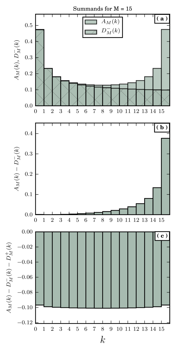
Now break the sum into two parts, which we denote as ( for bulk) and ( for fringe):
| (31) |
When the left-right symmetry is applied, this becomes
| (32) |
III.4 Bulk
To estimate the bulk sum, , we examine its summand , as shown in Fig. 1. By construction, ) decays at least as fast as as approaches 0, and similarly decays as approaches . Moreover, each of has a single singularity which cancels that at corresponding endpoint in . So in this sense, the sum does not inherit the singular behavior that the summand of once had, meaning that we can safely replace it with a corresponding midpoint integral at the cost of an error no larger than .
To begin, use the left-right symmetry to combine the sums:
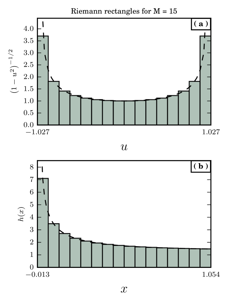
From Fig. 2(a) and Eq. (25), the first sum can be approximated by
To handle the second sum, regard
| (33) |
for as mesh points in the midpoint integral for , so that . Then from Fig. 2(b) and the first two terms of (30), we see that the second sum can be approximated by integrating
| (34) |
Thus
Here, in the second integral, the upper limit is the rightmost edge of the rightmost Riemann rectangle in Fig. 2(b). The integral must go up to this value to properly capture the terms. Evaluating the integrals gives
| (35) |
III.5 Fringe
Next we need to to estimate the fringe sum . Substitution of (30) for yields
| (36) |
All the sums above are variations on , whose asymptotics for large follow from results obtained in Refs. oliver10 ; vepstas07 . Those authors showed that, in general,
| (37) |
where is the Hurwitz zeta function (9). For our purposes, we evaluate the above with for , and . Inserting these results into (36) gives
| (38) |
III.6 Locking threshold
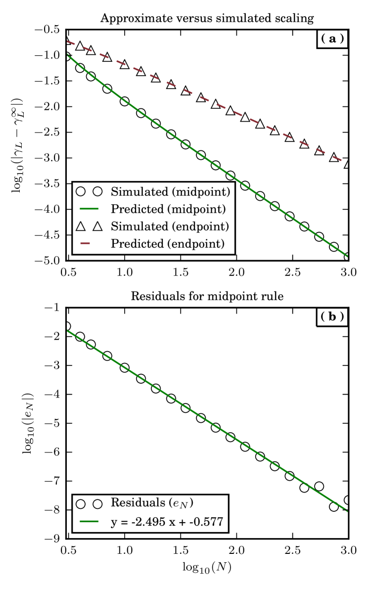
With the final piece of the puzzle in place, we can now derive an asymptotic approximation for the locking threshold . First recall that for the midpoint rule (3), the maximal frequency and the locking threshold are related via , from (8), whereas is related to the sum via , from (23); hence . To calculate , we add (35) and (38). Then becomes
This equation looks worrisome until one recalls the results of Bailey et al. bailey09 mentioned in the Introduction: satisfies and is related to by . Then the equation above for collapses to
| (39) |
where we have also made use of . The corresponding result for the endpoint rule is
| (40) |
In these equations, , which not only successfully recreates the scaling exponents found numerically pazo05 , but also gives the exact prefactors. Figure 3 shows that these predictions agree with numerics.
IV Discussion
An important thing to notice is that even though the midpoint rule (3) and the endpoint rule (4) both approach a uniform distribution on , their locking thresholds (their critical widths at which stable phase locking is lost) scale entirely differently. It is possible to blame this on analytic corrections to scaling, but that downplays the level of flexibility we have on the critical exponent.
For example, consider the following distribution of natural frequencies:
where and . Then, following our previous analysis, we find to leading order that . So in principle, the scaling exponent can be made as close to zero as we like (and the prefactor is equally flexible), despite this distribution also approaching the same uniform distribution as the two we have studied.
Interestingly, the opposite situation can also happen. Namely, consider the following distribution:
Numerically speaking, the will dominate the term for all , so this still approaches the uniform distribution from the inside. However, if we try to estimate the locking threshold for this case, we get
Now we get a distribution whose locking threshold has a critical exponent larger than what our approach above can estimate. In principle, we could do a more careful analysis using the and coefficients to be able to say exactly what the prefactor and coefficient should be in this case, but we will leave this as an exercise for the diligent student.
Research supported in part by a Sloan Fellowship to Bertrand Ottino-Löffler, and by NSF grants DMS-1513179 and CCF-1522054.
References
- (1) Y. Kuramoto, in International Symposium on Mathematical Problems in Theoretical Physics, H. Araki, ed., Lecture Notes in Phys. 39 (Springer, Berlin, 1975), p. 420.
- (2) Y. Kuramoto, Chemical Oscillations, Waves, and Turbulence (Springer, Berlin, 1984).
- (3) S. H. Strogatz, Physica D 143, 1 (2000).
- (4) A. Pikovsky, M. Rosenblum, and J. Kurths, Synchronization: A Universal Concept in Nonlinear Sciences (Cambridge University Press, 2003).
- (5) S. H. Strogatz, Sync (Hyperion, New York, 2003).
- (6) J. A. Acebrón, L. L. Bonilla, C. J. P. Vicente, F. Ritort, and R. Spigler, Rev. Mod. Phys. 77, 137 (2005).
- (7) F. Dörfler and F. Bullo, Automatica 50, 1539 (2014).
- (8) A. Pikovsky and M. Rosenblum, Chaos 25, 097616 (2015)
- (9) F. A. Rodrigues, T. K. DM. Peron, P. Ji and J. Kurths, Phys. Rep. 610, 1 (2016).
- (10) A. T. Winfree, J. Theor Biol. 16, 15 (1967).
- (11) H. Daido, J. Phys. A 20, L629 (1987).
- (12) H. Daido, Prog. Theor. Phys. 81, 727 (1989)
- (13) H. Daido, J. Stat. Phys. 60, 753 (1990).
- (14) H. Hong, H. Park, and M. Y. Choi, Phys. Rev. E 72, 036217 (2005).
- (15) H. Hong, H. Chaté, H. Park, and L.-H. Tang, Phys. Rev. Lett. 99, 184101 (2007).
- (16) H. Hong, H. Chaté, L.-H. Tang, and H. Park, Phys. Rev. E 92, 022122 (2015).
- (17) E. J. Hildebrand, M. A. Buice, and C. C. Chow, Phys. Rev. Lett. 98, 054101 (2007).
- (18) M. A. Buice and C. C. Chow, Phys. Rev. E 76, 031118 (2007).
- (19) G.B. Ermentrout, J. Math. Biol. 22, 1 (1985).
- (20) J.L. van Hemmen and W.F. Wreszinski, J. Stat. Phys. 72, 145 (1993).
- (21) A. Jadbabaie, N. Motee, and M. Barahona, in Proceedings of the American Control Conference, Boston, MA, 2004, p. 4296.
- (22) Yu. Maistrenko, O. Popovych, O. Burylko, and P. A. Tass, Phys. Rev. Lett. 93, 084102 (2004).
- (23) D. Aeyels and J. Rogge, Prog. Theor. Phys. 112, 921 (2004).
- (24) R.E. Mirollo and S.H. Strogatz, Physica D 205, 249 (2005).
- (25) D. Pazó, Phys. Rev. E 72, 046211 (2005).
- (26) D. Quinn, R. Rand, and S. H. Strogatz, Phys. Rev. E 75, 36218 (2007).
- (27) M. Verwoerd and O. Mason, SIAM J. Applied Dynamical Systems 7, 134 (2008).
- (28) M. Verwoerd and O. Mason, SIAM J. Applied Dynamical Systems 10, 906 (2011).
- (29) F. Dörfler and F. Bullo, SIAM J. Applied Dynamical Systems 10, 1070 (2011).
- (30) D. Bailey, J. Borwein, R. Crandall, Experimental Mathematics 18, 107 (2009).
- (31) N. Durgin, S. Garcia, T. Flournoy, D. Bailey, https://escholarship.org/uc/item/0kr400n1 (2008).
- (32) F. W. J. Olver, D. W. Lozier, R. F. Boisvert, and C. W. Clark, NIST Handbook of Mathematical Functions (Cambridge University Press, 2010).
- (33) L. Vepštas, http://arxiv.org/abs/math/0702243 (2007).