The time-dependent Aharonov-Casher effect

Abstract

In this paper we give a covariant expression for Aharonov-Casher phase. This expression is a combination of the canonical electric field, Aharonov-Casher phase plus a magnetic field phase shift. We use this covariant expression for the Aharonov-Casher phase to investigate the case of a neutral particle with a non-zero magnetic moment moving in the time dependent electric and magnetic fields of a plane electromagnetic wave background. We focus on the case where the magnetic moment of the particle is oriented so that both the electric and magnetic field lead to non-zero phases, and we look at the interplay between these electric and magnetic phases.

I Introduction

The Aharonov-Bohm (AB) effect AB ; ES and its experimental confirmation chambers ; tonomura are an important consequence of combining quantum mechanics with gauge theories. The basic AB set-up is the quantum mechanical two-slit experiment for charged particles but with a magnetic-flux-carrying infinite solenoid placed between the two slits. Even though there is no magnetic field outside the solenoid, there is a non-vanishing vector potential, which leads to a shift in the interference pattern formed by the charged particles going through the slits. However, this shift in the interference pattern depends only on the magnetic flux carried inside the solenoid. This gives the AB effect a non-local character since the phase of the particle is influenced by the magnetic field, which is zero at the location of the particle.

The closely related Aharonov-Casher (AC) effect AC ; anadan is also a modified version of the quantum mechanical two-slit experiment, but using neutral particles with a non-vanishing magnetic moment traveling through the slits with a line of charge placed between the slits. One again finds a quantum phase shift due to the presence of the electric field coming from the line of charge. This phase shift leads to an observable shift in the interference pattern cimmino .

The AC effect can be seen as the dual of the AB effect in the following sense: In the AB set-up one has a magnetic flux carrying solenoid, which can be pictured as a line of magnetic dipoles laid end-to-end, with electrically charged particles moving around the solenoid. A duality transformation exchanges the magnetic dipoles with the electric charge so that for the AC set-up one has a line of charges with neutral, magnetic dipoles moving around this line of charge. In both cases the particles pick up an additional quantum phase which manifests itself as a shift in the usual two-slit interference pattern.

Both the AB and AC effects are topological since they depend on the non-simply connected nature of each set-up. The infinite solenoid or the infinite line of charge exclude some region of the space-time so that the space is not simply connected (for more discussion on this point see ryder ). Further the AB effect has been connected to Berry Phases berry which are general “geometric” phases that arise in certain quantum systems.

While the time-independent AB and AC effects have been extensively studied both theoretically and experimentally, the same does not hold for the time-dependent cases when the magnetic flux in the solenoid or the electric charge on the wire are time-dependent. The theoretical predictions as to the outcome of a time-dependent AB experiment have been studied in chiao singleton singleton2 . There is some disagreement, theoretically, as to the outcome of the time-dependent AB effect. The authors of chiao predict that the interference pattern should shift with time according to the time dependence of the magnetic flux, whereas the authors of singleton singleton2 find a cancellation between the usual magnetic AB phase shift and the additional phase shift that arises due to the electric field that exists in the time-dependent case. The one experiment performed to date on the time dependent AB effect chentsov ; ageev did find no shifting of the interference pattern, but the parameters used in the set-up did not allow one to definitely conclude which prediction – a time dependent shifting of the interference pattern or little/no time dependent shifting of the interference pattern – is correct. Thus additional experiments are called for in the case of the time-dependent AB effect.

In this paper we write down a covariant version of the AC phase shift, and then use this expression to study the time-dependent AC effect. The covariant expression which we find for the Aharonov-Casher phase has some relationship to the geometrical phases obtained in casana from Lorentz-violating terms from fermion interaction from certain Standard Model extensions.

II Covariant expression for Aharonov-Casher Phase

In this section we begin by reviewing the derivation of the time-independent Aharonov-Casher phase AC and also the derivation of the Bernstein phase bernstein which is also known as the scalar Aharonov-Bohm phase. We use these two time-independent phases to give a motivation for our proposed expression for the covariant Aharonov-Casher phase, and then we give a more rigorous derivation of this covariant expression for the Aharonov-Casher phase.

In the original AC proposal AC (see also anadan for an earlier, closely related study) a neutral, spin-$\frac{1}{2}$ particle was taken to move through an electric field. In reference AC the neutral, spin-$\frac{1}{2}$ particle was taken to be a neutron and the electric field was taken to be that of an infinite line of charge. The non-relativistic Hamiltonian for this system is

$$H_{NR}=\frac{1}{2m}\left({\vec{p}}-{\vec{E}}\times{\vec{\mu}}\right)^{2}-\frac{\mu^{2}E^{2}}{m}~{},$$ (1)

where ${\vec{p}}=-i\nabla$ is the momentum operator and we have set $\hbar=1$. Also the vector magnetic moment is given as ${\vec{\mu}}=\mu{\vec{s}}$ (where the spin of the particle is ${\vec{s}}=\frac{1}{2}{\vec{\sigma}}$ with ${\vec{\sigma}}$ the standard Pauli matrices) and $E=|{\vec{E}}|$. The last term, $\frac{\mu^{2}E^{2}}{m}$, is negligible if $\mu E\ll mv$. The main point to note about (1) is that one can define an effective momentum operator ${\vec{p}}\rightarrow{\vec{p}}-{\vec{E}}\times{\vec{\mu}}$ analogously to the minimal coupling definition of the momentum operator for a particle with non-zero electric charge $e$ i.e. ${\vec{p}}\rightarrow{\vec{p}}-e{\vec{A}}$ with ${\vec{A}}$ being the 3-vector potential. This operator, ${\vec{p}}-e{\vec{A}}$, results in the additional AB phase for a charged particle moving along a path $L$ of the form

$$\Delta\alpha_{AB}=-e\int_{L}{\vec{A}}\cdot d{\vec{r}}~{}.$$ (2)

In the same way the operator, ${\vec{p}}-{\vec{E}}\times{\vec{\mu}}$, from (1) results in an additional AC phase for neutral particle with a magnetic moment moving along a path $L$

$$\Delta\alpha_{AC}=-\int_{L}({\vec{E}}\times{\vec{\mu}})\cdot d{\vec{r}}=-\mu\int_{L}({\vec{E}}\times{\vec{s}})\cdot d{\vec{r}}~{},$$ (3)

Next we move on to the Bernstein phase bernstein or the scalar AB effect. When a neutral particle with a magnetic momentum passes through a magnetic field the non-relativistic Hamiltonian for such a system is

$$H_{NR}=\frac{1}{2m}{\vec{p}}~{}^{2}-{\vec{\mu}}\cdot{\vec{B}}~{}.$$ (4)

It was shown by Bernstein bernstein that this Hamiltonian also results in a quantum phase shift if the magnetic moment, ${\vec{\mu}}$, moves through a magnetic field, ${\vec{B}}$. The additional phase picked up due to the ${\vec{\mu}}\cdot{\vec{B}}$ term in (4) can be written as

$$\Delta\alpha_{B}=\int_{L}({\vec{\mu}}\cdot{\vec{B}})dt=\mu\int_{L}({\vec{s}}\cdot{\vec{B}})\frac{dx}{v}~{},$$ (5)

where in the second integral the time integration has been turned into a space integration via $v=\frac{dx}{dt}$ where $v$ is the velocity of the particle. This is done to make the connection with the form of the Bernstein phase as given in the original paper bernstein . However, the main thing to note is that $\Delta\alpha_{AC}$ involves a spatial integration while $\Delta\alpha_{B}$ involves a time integration. This previews the eventual combination of these two phase shifts into a covariant space-time integral. The magnetic moment in (5) has again been split as ${\vec{\mu}}=\mu{\vec{s}}$. This phase shift given in (5) was experimentally observed by Werner et al. werner .

The phase shifts due to the electric field (the Aharonov-Casher effect) and magnetic field (the Bernstein effect) as written in equations (3) and (5) are in non-covariant, 3-vector notation. Here we suggest a 4-vector, covariant expression for the AC effect (which also therefore includes the Bernstein effect). The phase shifts in (3) and (5) can be combined and written covariantly via the expression

$$\Delta\alpha_{AC-B}=\mu\int{\cal F}_{\mu\nu}S^{\nu}dx^{\mu}~{},$$ (6)

where $\mu$ is the magnitude of the magnetic moment defined previously. The term ${\cal F}_{\mu\nu}$ is the dual Faraday field strength tensor ${\cal F}_{\mu\nu}=\frac{1}{2}\epsilon_{\mu\nu\alpha\beta}F^{\alpha\beta}$ with $\epsilon_{\mu\nu\alpha\beta}$ being the 4D anti-symmetric Levi-Civita symbol and $F^{\alpha\beta}=\partial^{\alpha}A^{\beta}-\partial^{\beta}A^{\alpha}$ is the Faraday field strength tensor. The term $S^{\nu}$ is the axial spin 4-vector (see the discussion in jackson ) which is given as

$$S^{\mu}=\left(\gamma{\vec{\beta}}\cdot{\vec{s}}~{},~{}{\vec{s}}+\frac{\gamma^{2}}{1+\gamma}({\vec{\beta}}\cdot{\vec{s}}){\vec{\beta}}\right)=(S^{0},{\vec{S}})~{},$$ (7)

with ${\vec{s}}=\frac{1}{2}{\vec{\sigma}}$ the standard 3-vector spin and $\gamma$, ${\vec{\beta}}$ the usual relativistic gamma and beta factors. In the low velocity limit $S^{\nu}\rightarrow(0,{\vec{s}})$, one can show that $\Delta\alpha_{AC-B}$ from (6) reduces to the sum of $\Delta\alpha_{AC}$ and $\Delta\alpha_{B}$ from (3) and (5). Using $S^{\nu}\rightarrow(0,{\vec{s}})$ one can split (6) into spatial and time integrals as

$$\Delta\alpha_{AC-B}=\mu\int\left({\cal F}_{ij}s^{j}dx^{i}+{\cal F}_{0j}s^{j}dx^{0}\right)~{}.$$ (8)

Where in the low velocity limit the 4-vector spin has become just the ordinary 3-vector spin. Combining this with the dual field strength tensor time-space component – ${\cal F}_{0j}=B_{j}$ – one finds that in the low velocity limit the integrand of the second term in (8) becomes $\mu{\cal F}_{0j}s^{j}\rightarrow{\vec{\mu}}\cdot{\vec{B}}$ where ${\vec{\mu}}=\mu{\vec{s}}$. Next for the dual field strength tensor the space-space components are ${\cal F}_{ij}=\epsilon_{ijk}E_{k}$. Combining this with low velocity limit for $S^{\nu}$ the integrand of the first term in (8) becomes $\mu{\cal F}_{ij}s^{j}\rightarrow\mu\epsilon_{ijk}s^{j}E_{k}\rightarrow\mu{\vec{s}}\times{\vec{E}}\rightarrow-{\vec{E}}\times{\vec{\mu}}$, which is just the integrand of the Aharonov-Casher phase in (3).

The above development is a motivation that the expression given in (6) is the covariant generalization of the Aharonov-Casher phase (3) and the Bernstein phase (5). It is possible to obtain this covariant phase more rigorously. As in the original work of Aharonov and Casher we start with the Dirac equation for a neutral particle non-minimally coupled to via its magnetic moment to the electromagnetic field, $F_{\mu\nu}$

$${\cal L}={\bar{\Psi}}\left(i\gamma^{\mu}\partial_{\mu}-\frac{\mu}{2}F_{\mu\nu}\sigma^{\mu\nu}-m\right)\Psi~{},$$ (9)

where $m$ is the mass of the particle, $\mu$ is the magnitude of its magnetic moment, $\gamma^{\mu}$ are Dirac matrices and $\sigma^{\mu\nu}=\frac{i}{2}[\gamma^{\mu},\gamma^{\nu}]$. Next we define the spin projection operators

$$\Sigma_{\pm}({\vec{S}})=\frac{1}{2}\left(1\pm\gamma^{5}\gamma^{\mu}S_{\mu}\right)~{}.$$ (10)

This operator projects out the $+{\vec{S}}$ and $-{\vec{S}}$ components of the spinor $\Psi$ along the direction ${\vec{S}}$ via the expressions

$$\Psi_{\pm}=\Sigma_{\pm}\Psi~{}~{}~{};~{}~{}~{}{\bar{\Psi}}_{\pm}=\Sigma_{\pm}{\bar{\Psi}}~{}.$$ (11)

Thus the spinor $\Psi$ can be decomposed as $\Psi=\Psi_{+}+\Psi_{-}$. The Lagrangian in (9) can now be written as

$${\cal L} = \left({\bar{\Psi}}_{+}+{\bar{\Psi}}_{-}\right)\left(i\gamma^{\mu}\partial_{\mu}-\frac{\mu}{2}F_{\mu\nu}\sigma^{\mu\nu}-m\right)\left(\Psi_{+}+\Psi_{-}\right)$$

$${\cal L}_{\pm} = {\bar{\Psi}}_{\pm}\left(i\gamma^{\mu}\partial_{\mu}-\frac{\mu}{2}F_{\mu\nu}\sigma^{\mu\nu}-m\right)\Psi_{\pm}~{}.$$ (12)

In the last line we note that the Lagrangian has split into two forms – ${\cal L}_{+}$ or ${\cal L}_{-}$ – depending on if one has ${\bar{\Psi}}_{+}\left(\cdots\right){\bar{\Psi}}_{+}$ or ${\bar{\Psi}}_{-}\left(\cdots\right){\bar{\Psi}}_{-}$. This split occurs since for the canonical Aharonov-Casher set-up the particle beam is polarized so that one has $\Psi_{+}$ or $\Psi_{-}$. This is the reason that in the Lagrangians in (II) does not have mixed terms like ${\bar{\Psi}}_{+}\left(\cdots\right){\bar{\Psi}}_{-}$ since the beam is either $\Psi_{+}$ or $\Psi_{-}$. Thus the Lagrangian in (II) has been split into two separate Lagrangians – one for $\Psi_{+}$ (i.e. ${\bar{\Psi}}_{+}\left(i\gamma^{\mu}\partial_{\mu}-\frac{\mu}{2}F_{\mu\nu}\sigma^{\mu\nu}-m\right)\Psi_{+}$) and one for $\Psi_{-}$ (i.e. ${\bar{\Psi}}_{-}\left(i\gamma^{\mu}\partial_{\mu}-\frac{\mu}{2}F_{\mu\nu}\sigma^{\mu\nu}-m\right)\Psi_{-}$).

We now want to work on the terms from (II) of the form ${\bar{\Psi}}_{\pm}\left(\frac{\mu}{2}F_{\mu\nu}\sigma^{\mu\nu}\right)\Psi_{\pm}$. First, we use the standard properties of Dirac matrices and the antisymmetry of $F_{\mu\nu}$ and $\sigma^{\mu\nu}$ to write $F_{\mu\nu}\sigma^{\mu\nu}=iF_{\mu\nu}\gamma^{\mu}\gamma^{\nu}$. Next we note that

$$\gamma^{\mu}\gamma^{\nu}=\left\{\Sigma_{\pm},\gamma^{\mu}\gamma^{\nu}\right\}\mp\eta^{\mu\nu}\gamma^{5}\gamma^{\alpha}S_{\alpha}\pm i\epsilon^{\alpha\beta\mu\nu}\gamma_{\beta}S_{\alpha}~{}.$$ (13)

Since we are interested in the term ${\bar{\Psi}}_{\pm}\left(\frac{\mu}{2}F_{\mu\nu}\sigma^{\mu\nu}\right)\Psi_{\pm}\rightarrow{\bar{\Psi}}_{\pm}\left(i\frac{\mu}{2}F_{\mu\nu}\gamma^{\mu}\gamma^{\nu}\right)\Psi_{\pm}$ we can drop $\eta^{\mu\nu}\gamma^{5}\gamma^{\alpha}S_{\alpha}$ from (13) since $F_{\mu\nu}$ is antisymmetric and $\eta^{\mu\nu}$ is symmetric. For the remaining terms, remembering $\Psi_{\pm}=\Sigma_{\pm}\Psi$, we apply $\Sigma_{\pm}$ to the left and right of $\gamma^{\mu}\gamma^{\nu}$ above to get

$$\Sigma_{\pm}\gamma^{\mu}\gamma^{\nu}\Sigma_{\pm} = \Sigma_{\pm}\left\{\Sigma_{\pm},\gamma^{\mu}\gamma^{\nu}\right\}\Sigma_{\pm}\pm i\Sigma_{\pm}\epsilon^{\alpha\beta\mu\nu}\gamma_{\beta}S_{\alpha}\Sigma_{\pm}$$

$$= 2\Sigma_{\pm}\gamma^{\mu}\gamma^{\nu}\Sigma_{\pm}\pm i\Sigma_{\pm}\epsilon^{\alpha\beta\mu\nu}\gamma_{\beta}S_{\alpha}\Sigma_{\pm}$$

$$= \mp i\Sigma_{\pm}\epsilon^{\alpha\beta\mu\nu}\gamma_{\beta}S_{\alpha}\Sigma_{\pm}~{},$$

where in the second line we have used the fact that $\Sigma_{\pm}$ is a projection operator i.e. $\Sigma_{\pm}\Sigma_{\pm}=\Sigma_{\pm}$. Putting all this together we can write the Lagrangians in (II) as

$${\cal L}_{\pm}={\bar{\Psi}}_{\pm}\left(\gamma^{\mu}[i\partial_{\mu}-\mu{\cal F}_{\mu\nu}S^{\nu}]-m\right)\Psi_{\pm}~{},$$ (15)

The Lagrangian of the usual minimally coupled Dirac particle with charge $e$ has the form ${\cal L}_{Dirac}={\bar{\Psi}}\left(\gamma^{\mu}[i\partial_{\mu}-eA_{\mu}]-m\right)\Psi$ with $A_{\mu}$ being the 4-vector potential. Comparing this Dirac Lagrangian with those in (15) we find the correspondence $eA_{\mu}\leftrightarrow\mu{\cal F}_{\mu\nu}S^{\nu}$ (this correspondence was also noted in dulat ). Then using the fact that the minimal coupling $i\partial_{\mu}-eA_{\mu}$ gives the covariant Aharonov-Bohm phase as $e\oint A_{\mu}dx^{\mu}$ we conclude that the coupling in (15), $i\partial_{\mu}-\mu{\cal F}_{\mu\nu}S^{\nu}$ gives the covariant Aharonov-Casher phase

$$\Delta\alpha_{AC-B}=\mu\int{\cal F}_{\mu\nu}S^{\nu}dx^{\mu}~{}.$$ (16)

This agrees with the previously given form in (6). However here we have derived the covariant Aharonov-Casher phase starting from the Lagrangian in (9), whereas previously we only gave a motivation for the covariant form of the AC phase via heuristic arguments starting from the 3-vector form of the Aharonov-Casher phase (i.e. - $\mu\int_{L}({\vec{E}}\times{\vec{s}})\cdot d{\vec{r}}$) and the 3-vector form of the Bernstein/scalar Aharonov-Bohm phase (i.e. $\int_{L}({\vec{\mu}}\cdot{\vec{B}})dt$).

We now use the expression in (8) to make two comments about the combined Aharonov-Casher and Bernstein effect.

First, from the (8) we can write the integrand as a total differential

$$d(\Delta\alpha_{AC-B})=\partial_{i}(\Delta\alpha_{AC-B})dx^{i}+\partial_{0}(\Delta\alpha_{AC-B})dx^{0}=\mu\left({\cal F}_{ij}s^{j}dx^{i}+{\cal F}_{0j}s^{j}dx^{0}\right)~{},$$

which gives the identities $\partial_{i}(\Delta\alpha_{AC-B})=\mu{\cal F}_{ij}s^{j}$ and $\partial_{0}(\Delta\alpha_{AC-B})=\mu{\cal F}_{0j}s^{j}$. Now by the equality of mixed partial derivatives $\partial_{0}\partial_{i}(\Delta\alpha_{AC-B})=\partial_{i}\partial_{0}(\Delta\alpha_{AC-B})$ we have

$$\partial_{0}(\mu{\cal F}_{ij}s^{j})=\partial_{i}(\mu{\cal F}_{0j}s^{j})~{}.$$ (17)

Using ${\cal F}_{ij}s^{j}=\epsilon_{ijk}E_{k}s^{j}=-{\vec{E}}\times{\vec{s}}$ and $\mu{\cal F}_{0j}s^{j}={\vec{B}}\cdot{\vec{s}}$. Plugging this into (17) yields

$$\frac{1}{c}\frac{d}{dt}({\vec{E}}\times{\vec{s}})=-\nabla({\vec{B}}\cdot{\vec{s}})~{}.$$ (18)

In (18) we were able to replace the partial time derivative by the full time derivative since

$$\frac{d}{dt}({\vec{E}}\times{\vec{s}})=\frac{d{\bf x}}{dt}\cdot\left[\nabla({\vec{E}}\times{\vec{s}})\right]+\frac{\partial}{\partial t}({\vec{E}}\times{\vec{s}})\approx\frac{\partial}{\partial t}({\vec{E}}\times{\vec{s}})~{},$$

since in the low velocity limit $\frac{d{\bf x}}{dt}\approx 0$. The result in (18) implies that the force on the neutral magnetic moment, ${\vec{\mu}}=\mu{\vec{s}},$ moving in the combined electric and magnetic field is zero in the low velocity limit. The vanishing of the classical force on the particle is one of the conditions of the AB and AC effects.

Second, the canonical Aharonov-Casher effect as given by the phase in (3) is non-dispersive i.e. the phase shift is independent of the velocity of the particle. This same non-dispersive feature holds for the Aharonov-Bohm effect as well. This is a crucial aspect of the Aharonov-Bohm effect since if a charged particle interacts directly with a magnetic field, ${\vec{B}}$, one will also in general get phase shifts due to the ${\vec{v}}\times{\vec{B}}$ forces on the particle. However the phase shifts associated with the ${\vec{v}}\times{\vec{B}}$ forces are explicitly velocity dependent and thus dispersive. Now for the covariant expression of the AC phase given in (6) or (8) we see that, if we do not make the low velocity limit, that the AC phase shift will depend on the velocity ${\vec{\beta}}$, and will in general be dispersive. Thus the non-dispersive nature of the Aharonov-Casher effect is a result of taking the low velocity limit. For the non-covariant forms of the Aharonov-Bohm phase of (2) or the Aharonov-Casher phase of (3), the non-dispersive character of these phases is one of their fundamental features. From the covariant expression of the phase in equation (6) one finds that there will in general be a velocity dependence due to the form of the $4$-spin in (7). Thus in general the AC effect is dispersive. In contrast the covariant AB phase given by $e\oint A_{\mu}dx^{\mu}$ is still independent of the particle velocity and is non-dispersive even if one relaxes the low velocity limit.

In the next section we will examine the case where a neutral particle with a magnetic moment moves in the background field of a plane electromagnetic wave. The plane wave has both electric and magnetic fields, and both fields lead to non-zero phases which have an interesting interplay with one another.

III Aharonov-Casher-Bernstein effect in a plane electromagnetic wave background

We now want to use the results of the previous section to study a specific example of the time-dependent Aharonov-Casher-Bernstein effect. In the original Aharonov-Casher paper and in the original Bernstein paper the electric and magnetic fields were static. For example, the original Aharonov-Casher setup was for the static electric field of an infinite line charge. If this line charge were allowed to varying in time then one would generate magnetic fields which would lead to additional phase shifts and therefore the simple 3-vector expression for the Aharonov-Casher phase, equation (3), would not be correct; one would need a covariant expression, such as our proposal in equation (8), in order to handle the additional phase shift coming from the time dependence of the fields.

The particular time varying electric and magnetic background we consider is a plane electromagnetic wave traveling in the $+z$ direction and polarized along the $x$ direction. The fields for this are

$${\vec{E}}=f(\omega t-kz){\hat{\bf x}}~{}~{}~{}~{};~{}~{}~{}~{}{\vec{B}}=f(\omega t-kz){\hat{\bf y}}$$ (19)

We have written the electric and magnetic fields in terms of arbitrary wave forms, but for concreteness one can take them to be sinusoidal e.g $f(\omega t-kz)=E_{0}\sin(\omega t-kz)$. We now use the covariant phase shift expression given in (8) to investigate the phase shift on a neutron moving in the background of the linearly polarized plane wave of (19). There are three choices for the direction of ${\vec{s}}$ (and therefore the direction of ${\vec{\mu}}$): ${\hat{\bf x}}$, ${\hat{\bf y}}$, or ${\hat{\bf z}}$. Choosing ${\vec{s}}\sim{\hat{\bf x}}$ gives ${\vec{E}}\times{\vec{s}}=0$ and ${\vec{B}}\cdot{\vec{s}}=0$ so we would get no additional phase shift for this case. If ${\vec{s}}\sim{\hat{\bf z}}$ then ${\vec{B}}\cdot{\vec{s}}=0$ while ${\vec{E}}\times{\vec{s}}\sim{\hat{\bf y}}$. In this case, if the particle follows a path along the $y$ direction with $d{\vec{r}}\sim{\hat{\bf y}}$, one gets a time varying AC phase shift from the electric field, but no Bernstein phase shift. The details of this time varying AC phase shift will depend on the details of the velocity of the particle and the frequency of the wave , $\omega$. The case ${\vec{s}}\sim{\hat{\bf y}}$ is the most interesting and most general since now both the Aharonov-Casher and Bernstein phase shifts are non-zero since ${\vec{E}}\times{\vec{s}}\neq 0$ and ${\vec{B}}\cdot{\vec{s}}\neq 0$. In this case one finds an interesting interplay between the two effects.

For the electromagnetic fields given by (19) and the spin in the direction ${\vec{s}}\sim{\hat{\bf y}}$, the combined Aharonov-Casher-Bernstein phase shift according to (3) (5) and (8) for the particle traveling with velocity $v$ in the $\pm z$-direction is (we restore a factor of $\frac{1}{c}$)

$$\Delta\alpha_{AC-B} = \frac{\mu}{c}\int{\cal F}_{\mu\nu}S^{\nu}dx^{\mu}=\frac{\mu}{c}\int_{L}({\vec{s}}\cdot{\vec{B}})c~{}dt-\frac{\mu}{c}\int_{L}({\vec{E}}\times{\vec{s}})\cdot d{\vec{r}}$$

$$= \frac{\mu}{2v}\int_{L}[f(\omega t-kz)]dz-\frac{\mu}{2c}\int_{L}[f(\omega t-kz)]{\hat{\bf z}}\cdot(\pm dz{\hat{\bf z}})$$

$$= \frac{\mu}{2c}\int_{0}^{L}[f(\omega t-kz)]\left(\frac{c}{v}\mp 1\right)dz~{}.$$

In the second line we have used $dt=dz/|{\bf v}|$ and the $\pm$ in the electric field contribution indicates if the particle is going along $\pm{\hat{\bf z}}$. The factor of $\frac{1}{2}$ comes from the spin half of the particle. Note that when the particle moves with the wave (i.e. for particles moving in the $+{\hat{\bf z}}$ direction) the magnetic and electric effects tend to cancel. This can be seen from the factor of $\frac{c}{v}-1$ in (III) which goes to zero as the particle velocity approaches $c$ i.e $v\sim c$. (However in this ultra-relativistic limit we would need to take into account the full 4-vector spin, $S^{\mu}$, rather than simply the 3-vector spin , ${\vec{s}}$, as we did in (III)). When the particle moves against the direction of the wave (i.e. for particles moving in the - ${\hat{\bf z}}$ direction) the magnetic and electric effects tend to add. This can be seen from the factor of $\frac{c}{v}+1$ in (III) which goes to $2$ as the particle velocity approaches $c$ i.e $v\sim c$. This cancellation or adding, depending on the direction of travel of the particle in comparison to that of the wave, was also found in the case of the time-dependent Aharonov-Bohm for plane waves bright .

We now use (III) to calculate the total Aharonov-Casher-Bernstein phase shift for two particles starting at $z=0$ and $t=0$ going out to $z=\pm\Delta z$ in time $t=\Delta t$, then turning around and returning to $z=0$ at time $t=2\Delta t$. The magnitude of the velocity of the particles is $|{\bf v}|=\frac{\Delta z}{\Delta t}$. The closed space-time path of the particles is shown in figure 1. One particle moves along paths $1+2$ and the other particle moves along the paths $3+4$. To get a closed space-time path we reverse the direction of the particle going along paths $3+4$ by multiplying the line integrals for these paths by a minus sign and then adding them to the line integrals from paths $1+2$. This is indicated in the figure by the reversal of the arrows along paths $3+4$.

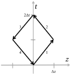
Figure 1: The closed space-time loop in the $t-z$ plane

Path 1 : For path 1 we have $z=vt$ and $\Delta z=v\Delta t$ so that the argument of the function $f$ becomes $\omega t-kz=\frac{\omega}{v}z-kz=k\left(\frac{c}{v}-1\right)z$, where we have used $\frac{\omega}{k}=c$. Now defining $k_{-}=k\left(\frac{c}{v}-1\right)$ the line integral for path 1 from (III) is

$$\frac{\mu}{c}\int_{1}{\cal F}_{\mu\nu}S^{\nu}dx^{\mu}=\frac{\mu}{2c}\left(\frac{c}{v}-1\right)\int_{0}^{\Delta z}f(k_{-}z)dz~{}.$$ (21)

Now defining $F(\zeta)=\int f(\zeta)d\zeta$ (e.g. if $f(\zeta)=E_{0}\sin(\zeta)$ then $F(\zeta)=-E_{0}\cos(\zeta)+K$) (21) integrates to

$$\frac{\mu}{c}\int_{1}{\cal F}_{\mu\nu}S^{\nu}dx^{\mu}=\frac{\mu}{2k_{-}c}\left(\frac{c}{v}-1\right)[F(k_{-}\Delta z)-F(0)]=\frac{\mu}{2\omega}[F(k_{-}\Delta z)-F(0)]~{},$$ (22)

where we have used $k_{-}=k\left(\frac{c}{v}-1\right)$ and $kc=\omega$.

Path 2 : For path 2 we have $z=-vt+2\Delta z$ and $\Delta t<t<2\Delta t$ so that $z$ goes from $z=\Delta z$ to $z=0$. The argument of the function $f$ becomes $\omega t-kz=2\Delta k\frac{c}{v}-k\left(\frac{c}{v}+1\right)z$. Now defining $k_{+}=k\left(\frac{c}{v}+1\right)$ the line integral for path 3 from (III) is

$$\frac{\mu}{c}\int_{2}{\cal F}_{\mu\nu}S^{\nu}dx^{\mu}=\frac{\mu}{2c}\left(\frac{c}{v}+1\right)\int^{0}_{\Delta z}f\left(2\Delta k\frac{c}{v}-k_{+}z\right)dz~{}.$$ (23)

Integration of (23) leads to

$$\frac{\mu}{c}\int_{2}{\cal F}_{\mu\nu}S^{\nu}dx^{\mu}=-\frac{\mu}{2\omega}\left[F\left(2k\Delta z\frac{c}{v}\right)-F(k_{-}\Delta z)\right]~{},$$ (24)

Note that while the integral in (23) begins with $k_{+}$ the final result has $k_{-}$.

Path 3 : For path 3 we have $z=vt-2\Delta z$ and $\Delta t<t<2\Delta t$ so that $z$ goes from $z=-\Delta z$ to $z=0$. The argument of the function $f$ becomes $\omega t-kz=2\Delta k\frac{c}{v}+k\left(\frac{c}{v}-1\right)z$. Recalling the definition $k_{-}=k\left(\frac{c}{v}-1\right)$ the line integral for path 3 from (III) is

$$\frac{\mu}{c}\int_{3}{\cal F}_{\mu\nu}S^{\nu}dx^{\mu}=\frac{\mu}{2c}\left(\frac{c}{v}-1\right)\int^{0}_{-\Delta z}f\left(2\Delta k\frac{c}{v}+k_{-}z\right)dz~{}.$$ (25)

Integration of (25) leads to

$$\frac{\mu}{c}\int_{3}{\cal F}_{\mu\nu}S^{\nu}dx^{\mu}=\frac{\mu}{2\omega}\left[F\left(2k\Delta z\frac{c}{v}\right)-F(k_{+}\Delta z)\right]~{},$$ (26)

The integral in (25) begins with $k_{-}$ the final result has $k_{+}$. A similar thing happened in the integration of path 2.

Path 4 : Finally, for path 4 we have $z=-vt$ and $\Delta z=-v\Delta t$ so that the argument of the function $f$ becomes $\omega t-kz=\frac{\omega}{c}z-kz=k\left(\frac{c}{v}+1\right)z$, where we have used $\frac{\omega}{k}=c$. Recalling $k_{+}=k\left(\frac{c}{v}+1\right)$ the line integral for path 4 from (III) is

$$\frac{\mu}{c}\int_{4}{\cal F}_{\mu\nu}S^{\nu}dx^{\mu}=\frac{\mu}{2c}\left(\frac{c}{v}+1\right)\int_{0}^{-\Delta z}f(-k_{+}z)dz~{}.$$ (27)

Integration of (27) leads to

$$\frac{\mu}{c}\int_{4}{\cal F}_{\mu\nu}S^{\nu}dx^{\mu}=-\frac{\mu}{2k_{+}c}\left(\frac{c}{v}+1\right)[F(k_{+}\Delta z)-F(0)]=\frac{\mu}{2\omega}[F(k_{+}\Delta z)-F(0)]~{},$$ (28)

where we have used $k_{+}=k\left(\frac{c}{v}-1\right)$ and $kc=\omega$.

We now combine the results from (22) (24) (26) (28) (remembering to put a minus sign in front of the results from path 3 and path 4 so that we get a closed space-time path) to get

$$\frac{\mu}{c}\oint{\cal F}_{\mu\nu}S^{\nu}dx^{\mu} = \frac{\mu}{c}\left(\int_{1}{\cal F}_{\mu\nu}S^{\nu}dx^{\mu}+\int_{2}{\cal F}_{\mu\nu}S^{\nu}dx^{\mu}+\int_{3}{\cal F}_{\mu\nu}S^{\nu}dx^{\mu}+\int_{4}{\cal F}_{\mu\nu}S^{\nu}dx^{\mu}\right)$$ (29)

$$= \frac{\mu}{\omega}\left[-F(0)-F\left(2k\Delta z\frac{c}{v}\right)+F(k_{+}\Delta z)+F(k_{-}\Delta z)\right]~{},$$

where $k_{\pm}=\left(1\pm\frac{c}{v}\right)$. Expanding the integration functions to second order $F(\eta)=F(0)+\eta F^{\prime}(0)+\frac{1}{2}\eta^{2}F^{\prime\prime}(0)+...$ gives for the loop integral in (29)

$$\frac{\mu}{c}\oint{\cal F}_{\mu\nu}S^{\nu}dx^{\mu}\approx\frac{\mu}{\omega}\left[F^{\prime\prime}(0)k^{2}\Delta z^{2}\left(1-\frac{c^{2}}{v^{2}}\right)\right]~{}.$$ (30)

The zero and first order terms cancel so that one finds that $\frac{\mu}{c}\oint{\cal F}_{\mu\nu}S^{\nu}dx^{\mu}$ is non-zero only starting at second order. A similar result was found in the case of the Aharonov-Bohm phase for a plane wave background bright . This result can be attributed to the interplay and partial cancellation between the electric and magnetic field contribution to the phases.

IV Summary and Conclusions

Here we have given a covariant expression for the Aharonov-Casher effect in equations (6) (16) as a generalization of the usual non-covariant 3-vector expression from (3). This covariant expression also includes the Bernstein or scalar Aharonov-Bohm phase shift. In 3-vector, non-covariant form the Bernstein phase is given in equation (5). One encounters the Bernstein/scalar Aharonov-Bohm effect when a neutral particle with a magnetic dipole moment moves through a magnetic field. One conclusion of the of the covariant expression (8) is that in general the Aharonov-Casher phase is dispersive i.e. depends on the velocity of the particle. This velocity dependence comes in through the form of the 4-vector spin, $S^{\mu}$, given in (7) which depends on ${\vec{\beta}}$. In contrast one of the hallmarks of the Aharonov-Bohm phase, $\frac{e}{\hbar c}\oint A_{\mu}dx^{\mu}$, is its non-dispersive character. As well the standard non-covariant, 3-vector Aharonov-Casher phase of (3) is velocity independent/non-dispersive.

The covariant expression of (6) (16) can be used to analyze situations where one has both electric and magnetic fields such as occurs generally in time dependent situations. Here we used the covariant expression to investigate the phase shift that occurs when a neutron moves in the background field of a plane, linearly polarized electromagnetic wave. The final result of the phase shift for this kind of background (and for the diamond path shown in figure 1) is that the time-dependent Aharonov-Casher phase vanishes to first order – from (30) we see that the first non-zero term comes from the second order term in the expansion of $F(\zeta)$. This approximate vanishing can be attributed to the interplay and partial cancellation between the electric and magnetic contributions to the phase. A similar partial cancellation between the electric and magnetic contributions to the phase has been seen in the case of the time-dependent Aharonov-Bohm effect singleton ; singleton2 ; bright .

Acknowledgments: DS is supported by a 2015-2016 Fulbright Scholars Grant to Brazil. DS wishes to thank the ICTP-SAIFR in São Paulo for it hospitality. DS also acknowledges support by a grant (number 1626/GF3) in Fundamental Research in Natural Sciences by the Science Committee of the Ministry of Education and Science of Kazakhstan.

References

- (1) Y Aharonov and D. Bohm, Phys. Rev. 115, 484 (1959).
- (2) W. Ehrenberg and R. E. Siday, Proc. Phys. Society B 62, 8 (1949).
- (3) R. G. Chambers, Phys. Rev. Lett. 5, 3 (1960).
- (4) A. Tonomura, et al., Phys. Rev. Lett. 56, 792 (1986).
- (5) Y. Aharonov and A. Casher, Phys. Rev. Lett., 53, 319 (1984).
- (6) J. Anandan, Phys. Rev. Lett., 48, 1660 (1982).
- (7) A. Cimmino, et al., Phys. Rev. Lett., 63, 380 (1989).
- (8) L. Ryder, Quantum Field Theory 2nd edition, section 3.4 (Cambridge Press, Cambridge UK 1996)
- (9) M.V. Berry, Proc. R. Soc. Lond. A392, 45 (1984).
- (10) B. Lee, E. Yin, T. K. Gustafson, and R. Chiao, Phys. Rev. A 45, 4319 (1992).
- (11) D. Singleton and E. Vagenas, Phys. Lett. B 723, 241 (2013).
- (12) J. MacDougall and D. Singleton, J. Math. Phys. 55, 042101 (2014).
- (13) J.D. Jackson, Classical Electrodynamics, 3rd edition, section 11.11 (John Wiley & Sons Inc., New York).
- (14) Yu. V. Chentsov, Yu. M. Voronin, I. P. Demenchonok, and A. N. Ageev, Opt. Zh. 8, 55 (1996).
- (15) A. N. Ageev, S. Yu. Davydov, and A. G. Chirkov, Technical Phys. Letts. 26, 392 (2000).
- (16) R. Casana, M.M. Ferreira, V.E. Mouchrek-Santos, and E. O. Silva, Phys.Lett. B 746, 171 (2015).
- (17) H. J. Bernstein, Phys. Rev. Lett., 18, 1102 (1967).
- (18) S.A. Werner, R. Colella, A. W. Overhauser, and C. F. Eagen, Phys. Rev. Lett., 35, 1053 (1975)
- (19) S. Dulat and K. Ma, Phys. Rev. Lett., 108, 070405 (2012)
- (20) A. Kholmetskii, O. Missevitch, and T. Yarman, Eur. Phys. J. Plus 129, 215 (2014).
- (21) M. Bright, D. Singleton and A. Yoshida, Eur. J. Phys. C 75, 446 (2015)