Ion-acoustic Shocks with Self-Regulated Ion Reflection and Acceleration

Abstract

An analytic solution describing an ion-acoustic collisionless shock, self-consistently with the evolution of shock-reflected ions, is obtained. The solution extends the classic soliton solution beyond a critical Mach number, where the soliton ceases to exist because of the upstream ion reflection. The reflection transforms the soliton into a shock with a trailing wave and a foot populated by the reflected ions. The solution relates parameters of the entire shock structure, such as the maximum and minimum of the potential in the trailing wave, the height of the foot, as well as the shock Mach number, to the number of reflected ions. This relation is resolvable for any given distribution of the upstream ions. In this paper, we have resolved it for a simple “box” distribution. Two separate models of electron interaction with the shock are considered. The first model corresponds to the standard Boltzmannian electron distribution in which case the critical shock Mach number only insignificantly increases from $M\approx 1.6$ (no ion reflection) to $M\approx 1.8$ (substantial reflection). The second model corresponds to adiabatically trapped electrons. They produce a stronger increase, from $M\approx 3.1$ to $M\approx 4.5$. The shock foot that is supported by the reflected ions also accelerates them somewhat further. A self-similar foot expansion into the upstream medium is also described analytically.

I Introduction

Collisionless shocks emerged in the 50s and 60s of the last century as an important branch of plasma physics (see Sagdeev66 ; tidman1971shock ; Kennel85 ; Papad85 for review) and have remained ever since. Meanwhile, new applications have posed new challenges to our understanding of collisionless shock mechanisms. Particle acceleration in astrophysical settings, primarily studied to test the hypothesis of cosmic ray origin in supernova remnant shocks (see, e.g., BlandEich87 ; MDru01 ; BlandfordCRorig2014 for review), stands out, and the collisionless shock mechanism is the key. Among recent laboratory applications, a laser-based tabletop proton accelerator is frequently highlighted as an affordable compact alternative to the expensive synchrotron accelerators, currently used to treat cancers Bulanov02 ; Haberberger2012NatPh ; FiuzaUCLA2013 .

The goal of this article is twofold. First, we will obtain a self-consistent analytic solution for the electrostatic structure of an ion-acoustic collisionless shock with the Mach numbers beyond a critical value $M=M_{*}\simeq 1.6$ (for Boltzmannian electrons, and $M_{*}\approx 3.1$ for adiabatically trapped electrons). At $M=M_{*},$ the shock is about to reflect some of the upstream ions. Second, we will study the dynamics of reflected ions, including their further acceleration. A self-similar simple wave solution for electrostatic potential in the foot region will be obtained selfconsistently with the incident and reflected ion dynamics. We will show that an additional drop in the foot electrostatic potential critically affects the ion reflection from the main part of the shock. So, unlike most of the earlier analyzes, treated the ion reflection using the test particle approximation, e.g., Medvedev09 ; FiuzaUCLA2013 , we incorporate it into the global shock structure. This study is relevant to the electrostatic shock propagation in laser-produced plasmas, especially to the problem of generation of monoenergetic ion beams, ion injection into the diffusive shock acceleration in astrophysical shocks, and other shock-related processes in astrophysical and space plasmas.

In non-isothermal plasmas, with the electron temperature much higher than ion temperature, $T_{e}\gg T_{i}$, a nonlinear Korteweg - de Vries (KdV) equation applies as long as the nonlinearity remains weak. Of course, the KdV equation is famous for its soliton solution, one of the most remarkable mathematical construction widely used in physics. In plasmas, the solitons emerge when neither collisional nor Landau damping is present. The ion-acoustic solitons, in particular, are the building blocks of collisionless shock waves at $T_{e}\gg T_{i}$. Most lucidly they emerge from a solution pseudopotential, for an arbitrarily strong nonlinearity, thus comprising the limiting case of a cnoidal wave solution with an infinite period Sagdeev66 . This solution can also be interpreted as the uppermost “energy level” in a continuum of bound states in the pseudopotential, whereas the lower energy bound states correspond to the periodic (cnoidal) waves. The use of pseudopotential also illuminates formation of a soliton wave-train, when even a small damping leads to the “particle” energy change in the pseudopotential which in reality corresponds to the inner structure of the shock front MoisSagd63 . The underlying mechanism here is the nonlinear Landau damping. Just a few ions upstream reflected by the electric potential of the first soliton will result in such damping. Then, by the “nonlinear saturation” effect, there are no more “resonant” ions to interact with the soliton train past the leading soliton.

In the absence of resonant ions upstream, the first soliton breaks down at $M>M_{*}\simeq 1.6$ (this particular number is valid for cold upstream ions and Boltzmann electrons). The solution ceases to exist beyond this point, as there is no proper “energy level” in the pseudopotential. This solution disappearance was thought to be the point of “overturning of the shock front” and the end of the so-called “laminar” regime of ion-acoustic collisionless shocks. However, the results of this paper prove otherwise. Namely, by including the reflected ions into the shock structure, we have found the laminar solution beyond $M=M_{*}$! More specifically, we found that when the ions begin to reflect from the soliton tip at $M=M_{1}\lesssim M_{*}$, the classical single soliton solution bifurcates into a more complex structure. It comprises (i) the first soliton, (ii) the infinite periodic wave train downstream of it, and (iii) the foot occupied by the reflected ions. The front edge of the foot undergoes self-similar spreading in a comoving reference frame of reflected ions. This solution continues up to $M=M_{2}\gtrsim M_{*}$.

At the second critical Mach number $M_{2}$, almost all incident ions reflect, so the foot potential raises to increase the total shock Mach number well above $M_{*}$. For the cold upstream ions, $T_{i}\ll T_{e}$, $M_{1}$ approaches $M_{*}$, that is $M_{1}=M_{*}-\mathcal{O}\left(\sqrt{T_{i}/T_{e}}\right)$, while $M_{2}\approx\sqrt{M_{*}^{2}+\left(1-1/4M_{*}^{2}\right)^{-1}\ln\left(1+\alpha\right)}$, where $\alpha$ is the fraction of reflected ions. Note that $M_{2}\approx 1.8$ for $\alpha=1$ and Boltzmannian electrons. The case of adiabatically trapped electrons, in which $M_{*}\approx 3.1$, gives a significantly higher Mach number, $M_{2}\approx 4.5$. The same pseudopotential technique Sagdeev66 , also recovers the shock profile, although by introducing two separate pseudopotentials $\Phi^{\pm}\left(\phi\right)=4\pi e\intop\left(n_{e}-n_{i}^{\pm}\right)d\phi$, used for the plasma upstream and downstream of the leading soliton ($n_{i}^{+}\neq n_{i}^{-}$ due to the ion reflection). Here $\phi$ denotes the shock electrostatic potential.

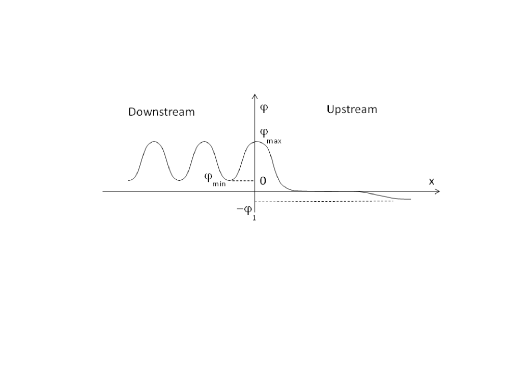
Figure 1: Electrostatic potential of the shock structure consisting of a pedestal, leading soliton and trailing wave

Within the range between the two critical points $M_{1}<M<M_{2}$, the only time-dependent part of the solution is near the leading edge of the reflected ion population. They support a pedestal upstream of the leading soliton on which it rests. The reflected ions escape upstream with double the shock speed in the pedestal reference frame, Fig.1. Their further fate is determined by a relatively slow spreading of the initially sharp front edge. By even a small velocity dispersion, ions with higher initial velocity undergo additional electrostatic acceleration by passing through the shock pedestal. This process is described analytically as a self-similar solution, which also yields the maximum velocity of reflected ions.

One usually employs two forms of electron density $n_{e}\left(\phi\right)$ in the pseudopotential. One form is the Boltzmannian, $n_{e}=n_{0}\exp\left(e\phi/T_{e}\right)$, which yields $M_{*}\approx 1.6$ Sagdeev66 . The other form corresponds to adiabatically trapped electrons, in which case $M_{*}\approx 3.1$ Gurevich68 . Depending on the practical situation either model can be used. The Boltzmannian requires a Maxwellian distribution for electrons trapped into potential wells (in analogy with barometric formula). One can expect such scenario in the case when a higher density plasma expands into a lower density (upstream) region. A suitable example found in the conventional gas dynamics is a shock tube, in which the shock is generated by breaking up a diaphragm, that was separating the areas with different densities. By contrast, the adiabatic trapping can be expected in a piston tube, in which the piston moves into an initially uniform medium. Therefore, it models the shocks generated in the pulsed laser-plasmas more accurately. Under these circumstances, the production of reflected ions can be considered as the laser-driven acceleration. It becomes more energy-efficient at $M>M_{*}$, while producing almost monoenergetic ions over an extended time interval.

The paper is organized as follows. In Sec.II we discuss the shock model. Sec.III describes the main part of the shock transition that forms in place of the parent soliton after it has reflected a first few ions. Sec.IV presents a self-similar solution for the shock precursor supported by reflected ions. We conclude with a Discussion in Sec.V.

II The Shock Model

The analytic solution for an ion-acoustic soliton was first obtained for the Boltzmannian electron distribution Sagdeev66 and extended later to the case of adiabatically trapped electrons Gurevich68 . Ions were assumed to be cold in both instances, which strictly limited the maximum Mach numbers to $M_{*}\simeq 1.6$ and $M_{*}\simeq 3.1$ for the Boltzmann and adiabatic electrons, respectively. When the Mach number reaches the maximum, the soliton begins to reflect some of the upstream ions and the shock model must include them. Unlike the soliton, the shock profile resulting from the ion reflection is asymmetric about the reflection point. As shown in Ref.MoisSagd63 , its downstream part oscillates. Upstream of the soliton, reflected ions will create a foot with an elevated electrostatic potential.

Seeking to extend the analytic solution beyond the ion reflection point, we need a manageable reflection model. At a minimum, the model should be able to relate the shock potential $\phi_{{\rm max}}$ and Mach number $M$ to the number of reflected ions. Therefore, the model must be kinetic, so one obtains the shock potential given the shock speed and upstream ion distribution with a finite temperature. If the ion temperature upstream was zero ($V_{Ti}=0$) the ions would reflect all at once when the shock Mach number crosses the point $M=$$\sqrt{2e\phi_{{\rm max}}/T_{e}}$. By contrast, if $V_{Ti}\neq 0$, then the reflection parameter $\alpha=n_{{\rm refl}}/n_{{\rm\infty}}$, which is the ratio of reflected ion density to that of the incident ions far away from the soliton, will continuously depend on the shock parameters $M$ and $\phi_{{\rm max}}$. The region ahead of the shock filled with the reflected ions of constant density (foot of the shock) is mathematically regarded as “infinity” in the treatment of the main part of the shock transition. There, all the relevant quantities, such as the electrostatic potential $\phi$ are considered asymptotically constant. The shock foot (precursor) will obviously expand linearly with time after the first ions are reflected. In considering the main part of the shock transition, we will count the plasma potential from its value in the foot, so that we set the potential at “infinity” to $\phi=0$ in this section. Turning to the transition near the leading edge of reflected ions in Sec.IV, we will account for the foot potential $\phi_{1}$ in the solution obtained in this section, Fig.1.

To describe ion reflection we use a simple generalization of a cold ion distribution upstream that provides an ion reflection model satisfying the above requirements. So we use a “box” ion distribution with the finite thermal velocity defined as $V_{Ti}=v_{2}-v_{1}$:

$$f_{i}^{\infty}\left(v\right)=\frac{1}{v_{2}-v_{1}}\begin{cases}1,&-v_{2}<v<-v_{1}\\ 0,&v\notin\left(-v_{2},-v_{1}\right)\end{cases}$$ (1)

The normalization of $f_{i}^{\infty}$ implies a unity density of incident ions far enough from the shock but not farther than the slowest particles in the leading group of reflected ions at a given time, as we discussed earlier. We use the shock frame throughout this section. It is convenient to introduce a dimensionless potential by replacing $e\phi/T_{e}\to\phi$ and measure the coordinate in units of $\lambda_{D}=\sqrt{T_{e}/4\pi e^{2}n_{\infty}}$, while the ion velocity in units of the sound speed, $C_{s}=\sqrt{T_{e}/m_{i}}$.

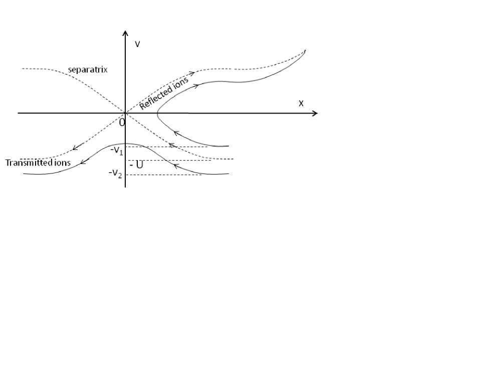
Figure 2: Phase plane of ions at reflection point and propagation of reflected ion beam accompanied by its further acceleration into the upstream medium and narrowing its velocity distribution at large $x$.

Suppose the soliton propagates in the positive $x$- direction with a nominal speed $U=\sqrt{2\phi_{{\rm max}}}$ (w.r.t. the foot), where $\phi_{{\rm max}}=\phi\left(0\right)$ is the maximum of its potential, and $v_{1}\leq U\leq v_{2}$. The ion density upstream and downstream can then be written as follows, Fig.2

$$n_{i}\left(\phi\right)=\frac{1}{v_{2}-v_{1}}\begin{cases}\sqrt{v_{2}^{2}-2\phi}-\sqrt{U^{2}-2\phi},&x\leq 0\\ \sqrt{v_{2}^{2}-2\phi}+\sqrt{U^{2}-2\phi}-2\sqrt{v_{1}^{2}-2\phi,}&x>0,\quad 0<\phi<v_{1}^{2}/2\\ \sqrt{v_{2}^{2}-2\phi}+\sqrt{U^{2}-2\phi}&x>0,\quad v_{1}^{2}/2\leq\phi\leq U^{2}/2\end{cases}$$ (2)

Again, we count the electrostatic potential from its value in the shock foot. We note that $U$ is not precisely the soliton velocity but rather a convenient notation for $\sqrt{2\phi_{{\rm max}}}$, while the soliton velocity with respect to the foot plasma (Mach number in this reference frame) is $M=\left(v_{1}+v_{2}\right)/2$. The soliton speed in the upstream plasma frame can only be determined when the foot potential $\phi_{1}$ is obtained, Fig.1. It is also important to note here that our choice of the simplest form of ion distribution, eq.(1) resulting in the ion density including the reflected ions should lead to the same shock structure in the limit $V_{Ti}\to 0$ as in the case of, say, Maxwellian distribution. In the latter case, the ion density in eq.(2) would be expressed through the error function. However, the limit $V_{Ti}\to 0$ can only be taken after the solution for the shock profile is obtained.

From this point on, our treatment will depend on the particular electron model, Boltzmannian or adiabatically trapped electrons. In the next two subsections, these two models are considered separately.

II.1 Boltzmannian Electrons

Based on the above definitions, the Poisson equation for the shock electrostatic potential can be written as follows

$$\frac{d^{2}\phi}{dx^{2}}=\left(1+\alpha\right)e^{\phi}-n_{i}\left(\phi\right)$$ (3)

where

$$\alpha=\frac{U-v_{1}}{v_{2}-v_{1}}$$ (4)

is the fraction of ions reflected off the shock, so that the first term on the r.h.s of eq.(3) corresponds to the electron contribution. We have chosen its normalization in such a way as to neutralize the sum of the incident and reflected ions in the foot, according to their normalization in eq.(1). We may now integrate eq.(3) once, also imposing the condition $\phi^{\prime}\left(\phi_{{\rm max}}\right)=0$. The resulting equation takes the following form

$$\frac{1}{2}\left(\frac{d\phi}{dx}\right)^{2}=\Phi\left(\phi\right)+\mathcal{F}^{\pm}\left(\phi\right)\equiv\Phi^{\pm}\left(\phi\right)$$ (5)

where ${}^{\prime}+^{\prime}$ or ${}^{\prime}-$’ sign should be taken for $x\geq 0$ and $x<0$, respectively. The functions $\Phi$ and $\mathcal{F}^{\pm}$ are given by the following relations

$$\Phi=\left(1+\alpha\right)\left(e^{\phi}-e^{U^{2}/2}\right)+\frac{\left(v_{2}^{2}-2\phi\right)^{3/2}-\left(v_{2}^{2}-U^{2}\right)^{3/2}}{3\left(v_{2}-v_{1}\right)}$$ (6)

$$\mathcal{F}^{\pm}=\frac{1}{3\left(v_{2}-v_{1}\right)}\begin{cases}\left(U^{2}-2\phi\right)^{3/2}-2\left(v_{1}^{2}-2\phi\right)^{3/2}\vartheta\left(v_{1}^{2}-2\phi\right),&x\geq 0\\ -\left(U^{2}-2\phi\right)^{3/2},&x<0\end{cases}$$ (7)

where $\vartheta$ is a Heaviside function. These relations are written for the case $U\geq v_{1}$, while the opposite case would correspond to the standard soliton solution with no ion reflection but with finite upstream ion temperature, which we do not consider in this paper. It is convenient to refer to the functions $\Phi^{\pm}\left(\phi\right)$ as to pseudopotentials of anharmonic oscillators of unit masses, whose kinetic and potential energies correspond, respectively, to the l.h.s. and the r.h.s of eq.(5). Here, $\phi$ represents the oscillator coordinate and $x$ represents time Sagdeev66 . The shock structure $\phi\left(x\right)$ is thus completely determined by eq.(5) in a form of an inverse function $x\left(\phi\right)$ under an appropriate choice of its branches upstream and downstream. In the next section, we specify the critical parameters of the shock profile $\phi_{{\rm max}}$ and $\phi_{{\rm min}}$, depending on the upstream ion temperature and Mach number. Again, by “upstream” we mean here the shock foot region where $\phi=0,$ Fig.1.

II.2 Adiabatically Trapped Electrons

Boltzmann distribution for electrons near the shock that we considered above is not always the best choice. If they drive the shock by themselves, the shock may confine them, at least in part, to the downstream side by trapping them in its potential. The trapped electrons acquire then a flat distribution while the free electrons maintain their Maxwellian distribution Gurevich68 . Hence, the following electron density distribution replaces the Boltzmann distribution in the Poisson equation given by eq.(3):

$$\frac{d^{2}\phi}{dx^{2}}=\left(1+\alpha\right)\frac{F\left(\phi+\phi_{1}\right)}{F\left(\phi_{1}\right)}-n_{i}\left(\phi\right),$$ (8)

where

$$F\left(\phi\right)\equiv e^{\phi}{\rm erfc}\sqrt{\phi}+2\sqrt{\phi/\pi}$$

while the ion distribution remains the same as in eqs.(2,3). In deriving eq.(8) we assumed electrons with negative energy $E_{e}=mv^{2}/2-e\phi\left(x\right)\leq 0$ to remain on the downstream side of the shock structure, where their distribution $f_{0}$ is constant, while the rest of the electrons obey the standard Maxwell-Boltzmann distribution. Apart from the normalization factor that accounts for the ion reflection rate $\alpha$ and the finite shock foot potential $\phi_{1}$, this distribution is identical to that used by Gurevich in Ref. Gurevich68 for collisionless electrons trapped into a soliton. Similarly to eq.(5), the first integral of the Poisson equation can be written as follows

$$\frac{1}{2}\left(\frac{d\phi}{dx}\right)^{2}=\Phi_{a}\left(\phi\right)+\mathcal{F}^{\pm}\left(\phi\right)\equiv\Phi_{a}^{\pm}\left(\phi\right)$$

where

$$\Phi_{a}\left(\phi\right) = \left(1+\alpha\right)\frac{F\left(\phi+\phi_{1}\right)-F\left(\phi_{{\rm max}}+\phi_{1}\right)-\frac{4}{3\sqrt{\pi}}\left[\left(\phi+\phi_{1}\right)^{3/2}-\left(\phi_{{\rm max}}+\phi_{1}\right)^{3/2}\right]}{F\left(\phi_{1}\right)}$$ (9)

$$+ \frac{\left(v_{2}^{2}-2\phi\right)^{3/2}-\left(v_{2}^{2}-U^{2}\right)^{3/2}}{3\left(v_{2}-v_{1}\right)}$$ (10)

and $\mathcal{F}^{\pm}$ is given by eq.(7). Again, we have added an integration constant to ensure that $d\phi/dx=0$ at $\phi=\phi_{{\rm max}}$. Once the shock model is defined for the two types of electron distribution, we proceed with the solutions for the respective shock structures.

III Solution for the main part of the shock transition

III.1 Boltzmannian Electrons

An implicit solution for the potential $\phi\left(x\right)$ in the regions $x\gtrless 0$ may be written using eq.(5) by the following inverse relations for $x\left(\phi\right)$

$$x\left(\phi\right)=\pm\frac{1}{\sqrt{2}}\intop_{\phi}^{\phi_{{\rm max}}}\frac{d\phi^{\prime}}{\sqrt{\Phi^{\pm}\left(\phi^{\prime}\right)}}$$ (11)

At the point where ions are about to reflect off the soliton tip, that is when $U=v_{1}$ ($\alpha=0$), two pseudopotentials are equal, $\Phi^{+}=\Phi^{-}.$ Therefore, the (soliton) solution remains symmetric, as it has to be in the case with no ion reflection. It is selected by imposing an additional constraint on the pseudopotential $\Phi^{+}$. Namely, $\Phi^{+}\left(\phi\right)$ must have a double root at $\phi=0$: $\Phi^{+}\left(0\right)=0$, $\Phi^{+\prime}\left(0\right)=0$ regardless of $\alpha$ being zero or positive. Note that the second condition, $\Phi^{+\prime}\left(0\right)=0$ is satisfied automatically via our choice of normalization of electron contribution, eq.(3), that ensures charge neutrality at $+\infty$. The condition $d\phi/dx=0$ at $x=\infty$, that amounts to $\Phi^{+}\left(\phi=0\right)=0$, yields the following nonlinear dispersion relation for the shock

$$\left(1+\alpha\right)\left(e^{U^{2}/2}-1\right)=\frac{v_{2}^{3}+U^{3}-2v_{1}^{3}-\left(v_{2}^{2}-U^{2}\right)^{3/2}}{3\left(v_{2}-v_{1}\right)}$$ (12)

Indeed, this is a relation between the shock amplitude $\phi_{{\rm max}}=U^{2}/2$ and its speed (Mach number w.r.t shock foot) $M=\left(v_{1}+v_{2}\right)/2$, just as in the case of conventional ion-acoustic soliton of Ref.Sagdeev66 . An important difference, however, is that this relation also includes the ion reflection coefficient $\alpha=\left(U-v_{1}\right)/\left(v_{2}-v_{1}\right)$ and the upstream velocity dispersion $V_{Ti}=v_{2}-v_{1}$, through which the upstream ion bounding velocities $v_{1}$ and $v_{2}$ in eq.(12) may always be expressed. In particular, $M=U+\left(1-2\alpha\right)V_{Ti}$. Assuming that $V_{Ti}\ll U$, from eq.(12) we obtain

$$e^{U^{2}/2}-1-U^{2}=-\frac{1}{3}\left(2U\right)^{3/2}\frac{\left(1-\alpha\right)^{3/2}}{1+\alpha}V_{Ti}^{1/2}$$ (13)

The left hand side (l.h.s.) of this relation is identical to the soliton dispersion relation (l.h.s.=0) taken at the ion reflection potential ($\phi_{{\rm max}}=U^{2}/2$). Therefore, the ion reflection does not change the shock speed w.r.t. the shock precursor in a plasma with cold ions upstream, $V_{Ti}\to 0$. Comparing eqs.(12) with (13) we see how this results from canceling out of the factor $1+\alpha$. However, the shock speed does grow with ion reflection rate $\alpha$ w.r.t. the upstream frame (since the precursor height $\phi_{1}$ grows as well), which we discuss later. It is also interesting to observe that the thermal correction to the shock speed diminishes with an increase in ion reflection, $\alpha\to 1$.

Neglecting the r.h.s. (cold upstream ions, $V_{Ti}\to 0$, or $\alpha\to 0$) gives the solution for the critical Mach number $U=M_{*}\approx 1.6$ Sagdeev66 . For a finite $V_{Ti}\ll v_{1,2}$ and arbitrary $\alpha<\alpha_{c}\approx 1$ (see below), we obtain the following dispersion relation

$$U\approx M_{*}-\frac{2^{3/2}}{3}\frac{\left(1-\alpha\right)^{3/2}M_{*}^{1/2}V_{Ti}^{1/2}}{\left(1+\alpha\right)\left(M_{*}^{2}-1\right)}$$ (14)

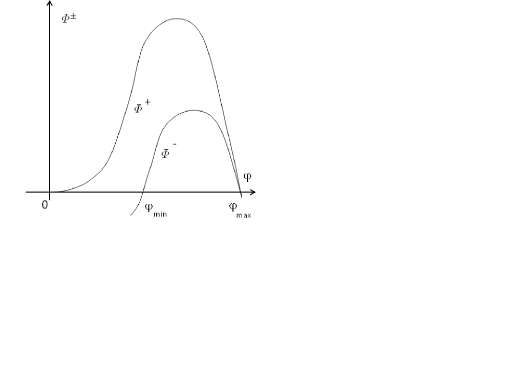
Figure 3: Pseudopotentials of “oscillators” described by eq.(5).

Turning to the spatial profile of the potential downstream ($x<0$), from eq.(5) and Fig.3 we see that it oscillates between its minimum value $\phi_{{\rm min}}$ and $\phi_{{\rm max}}=U^{2}/2$ that is given by eq.(14). Similarly to the above equation for $\phi_{{\rm max}}$, given by eq.(13), from eq.(5) we obtain the following equation for $\phi_{{\rm min}}$

$$e^{U^{2}/2}-e^{\phi_{{\rm min}}}=\frac{\left(v_{2}^{2}-2\phi_{{\rm min}}\right)^{3/2}-\left(U^{2}-2\phi_{{\rm min}}\right)^{3/2}-\left(v_{2}^{2}-U^{2}\right)^{3/2}}{3\left(1+\alpha\right)\left(v_{2}-v_{1}\right)}$$ (15)

The solution for $\phi_{{\rm min}}$ simplifies for the cases of weak and strong reflection. So, for $\alpha\ll 1$, using also eq.(14) we find

$$\phi_{{\rm min}}\simeq\frac{2M_{*}^{2}\sqrt{\alpha}}{\sqrt{M_{*}^{2}-1}}$$

The opposite case of strong reflection, $1-\alpha\ll 1$, should be treated with care when the small parameter $1-\alpha$ approaches the thermal spread of incident ions, $V_{Ti}$. First, assuming that $V_{Ti}\ll 1-\alpha\ll 1$, we obtain

$$\phi_{min}\simeq\phi_{max}-\frac{2M_{*}^{2}\left(1-\alpha\right)^{2}}{\left(1+M_{*}^{2}\right)^{2}}$$

For smaller $1-\alpha$ we may write

$$\phi_{min}\simeq\phi_{max}-\frac{9}{4}\left(1-\alpha\right)V_{T_{i}}M_{*}\left[1-\sqrt{\frac{V_{Ti}}{2\left(1-\alpha\right)}}\frac{\left(1+M_{*}^{2}\right)}{\sqrt{M_{*}}}\right]^{2}$$ (16)

The last solution cannot be continued to $\alpha=1$, as $\phi_{{\rm min}}$ reaches $\phi_{{\rm max}}$ at

$$\alpha=\alpha_{c}\simeq 1-V_{Ti}\left(1+M_{*}^{2}\right)^{2}/2M_{*}<1$$ (17)

It is not difficult to understand why there is no solution corresponding to complete ion reflection as $\alpha_{c}\neq 1$. Indeed, a solution with all particles reflected from the shock would nevertheless require a finite density downstream (to neutralize electrons), which could be possible only if the incident ions had no velocity dispersion (that is why $1-\alpha_{c}\sim V_{Ti}$ in eq.[17]). Therefore, when $\alpha$ increases to $\alpha=\alpha_{c}$, a solution $\phi\left(x\right)\equiv\phi_{{\rm max}}=const$ establishes downstream (pure shock transition). Instead of using eqs.(12) and (16), this special solution is easier to find directly by requiring charge neutrality condition fulfilled identically downstream, eq.(3)

$$e^{U^{2}/2}=\frac{1-\alpha}{1+\alpha}\sqrt{\frac{2U}{V_{Ti}\left(1-\alpha\right)}+1}.$$

This result, in combination with eq.(13), yields the critical value $\alpha=\alpha_{c}$ in eq.(17). Under this condition, the maximum potential $\phi_{{\rm max}}=U^{2}/2$ is determined by

$$U=M_{*}-\frac{V_{Ti}^{2}}{3M_{*}^{2}}\frac{\left(M_{*}^{2}+1\right)^{3}}{M_{*}^{2}-1}.$$ (18)

Together with eq.(14), the latter expression constrains the range of the shock Mach numbers for $0<\alpha<\alpha_{c}\approx 1$. These values of the shock potential and Mach number ($\simeq U$) relate to the upstream region occupied by reflected ions (where $\phi=0$). This region is located to the right from the leading soliton, but not farther than the slowest ions out of those that have been reflected first, Fig.1. A more precise meaning of this condition will be given in the next section. Now we turn to the calculation of the shock parameters for adiabatically trapped electrons.

III.2 Adiabatically Trapped Electrons

The calculation of shock characteristics for adiabatically trapped electrons is similar to that for the Boltzmannian electrons, but with one significant difference: the foot potential $\phi_{1}$ explicitly enters the Poisson equation also for the main part of the shock transitioin, cf. eqs.(3,8). Therefore, unlike in the Boltzmannian case, where the ion reflection rate $\alpha$ explicitly enters the shock solution only in conjunction with the incident ion thermal spread (see, e.g., eq.[14]), in the case of adiabatically trapped electrons the ion reflection effect is significantly stronger. The foot elevation $\phi_{1}$ is the largest contributing factor to that. Although, the latter is also determined by $\alpha$ that we will discuss in the next section.

Turning now to the shock solution, for its potential $\phi_{{\rm max}}\equiv U^{2}/2$ we obtain from eq.(9) the following relation:

$$\frac{F\left(\phi_{{\rm max}}+\phi_{1}\right)+\frac{4}{3\sqrt{\pi}}\left[\left(\phi_{{\rm max}}+\phi_{1}\right)^{3/2}-\phi_{1}^{3/2}\right]}{F\left(\phi_{1}\right)}-1-2\phi_{{\rm max}}=-\frac{2^{9/4}}{3}\phi_{{\rm max}}^{3/4}\frac{\left(1-\alpha\right)^{3/2}}{1+\alpha}V_{Ti}^{1/2}$$ (19)

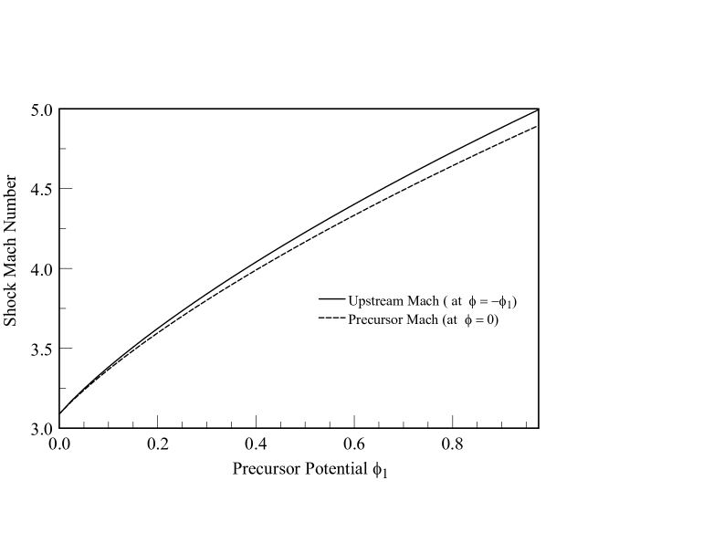
Figure 4: Solution of eq.(19) in the limit $V_{Ti}=0$ shown in the form of the shock Mach number related to the upstream frame, $M$, and to the foot ion reference frames, $U=\sqrt{2\phi_{{\rm max}}}$ (see text).

Unlike in the Boltzmann case, where the shock amplitude $\phi_{{\rm max}}$ was given by just a number $M_{*}^{2}/2$ in the limit $V_{Ti}\to 0$, now $\phi_{{\rm max}}$ depends directly on $\phi_{1}$. This dependence can be determined by solving eq.(19) numerically for $V_{Ti}\to 0$, as the major contributing factor is $\phi_{1}$. Fig.4 shows this solution in the form of the shock Mach number related to the far upstream medium and to the shock precursor, where $\phi=0$. The latter is given by the relation $U\left(\phi_{1}\right)=\sqrt{2\phi_{{\rm max}}}$, shown with the dashed line. As expected, it starts from the value $U\approx 3.1$, which is the maximum speed of a non-reflecting soliton calculated by Gurevich Gurevich68 . As the ion reflection rate $\alpha$ increases, so do $\phi_{1}\left(\alpha\right)$ and $U$.

To calculate the shock Mach number in the far upstream reference frame rather than the foot frame, one has to take into account the foot potential $\phi_{1}$. Indeed, the incident ions first slow down by passing through the potential $\phi_{1}$ before they hit the leading soliton in the shock structure and specularly reflect off it. The total Mach number (i.e. the absolute shock speed, again, given for $V_{Ti}\to 0$) then amounts to

$$M=2^{3/2}\sqrt{\phi_{{\rm max}}+\phi_{1}/4}-\sqrt{2\phi_{{\rm max}}}\approx\sqrt{2\phi_{{\rm max}}+\phi_{1},}$$ (20)

where the last expression is an approximation for $\phi_{1}\ll 2\phi_{{\rm max}}$ which holds up reasonably well for even a strong ion reflection. This dependence is shown in Fig.4 with the solid line. We see from the last equation that the direct effect of the foot elevation $\phi_{1}$ on the total Mach number is quite small, so that in the case of Boltzmannian electrons, where $\phi_{{\rm max}}$ does not depend on $\phi_{1}$ explicitly (eq.[12]) the maximum Mach number remains close to $M_{*}$. The dependence of the Mach number on $\alpha$ is considerably stronger for adiabatically trapped electrons, where $\phi_{{\rm max}}$ explicitly depends on $\phi_{1}\left(\alpha\right)$.

Now that we have obtained the shock structure up the location of first reflected ions, we turn to the dynamics of these ions. Obviously, they are at the front end of the shock precursor, where the shock potential drops to its upstream value. Depending on the time elapsed from the moment when the first ion reflection occurred, this area may be far away from the main part of the entire shock structure. Therefore, the assumption about the adiabatic trapping of electrons may not be justified there, so we restrict our calculation of $\phi_{1}$ to the case of Boltzmannian electrons. In the next section, we will relate the foot potential $\phi_{1}$ to $\alpha$. This relation provides the shock parameters depending only on the reflection parameter $\alpha$, by using eq.(20) and Fig.4.

IV Solution for the ion precursor

As we have seen, in the case of $\alpha>0$ the shock propagates through a foot region with the electrostatic potential elevated to $\psi=\phi_{1}$ from its level $\psi=0$ at $+\infty$. By entering this area the incident ions slow down before they encounter the leading soliton. It is convenient to account for this change in the shock structure potential by shifting the variable $\phi$ used in the previous sections to $\psi$ as follows $\psi=\phi+\phi_{1}$. So, we now focus on that part of the shock transition where $\psi$ varies in the interval $0<\psi<\phi_{1}$, Fig.1. From the physics perspective, one may assume that after an initial propagation of the reflected beam upstream, a quasi-steady flow at a constant speed and potential $\psi=\phi_{1}$ will be established between the ion-reflecting soliton and the head of the beam. Our consideration of the beam dynamics below (see, in particular, Appendix) implies that this assumption is not justified if the beam reflection is not strictly stationary, so the beam may continue to evolve all the way through its extension. However, under a stationary reflection most of the beam will also be stationary, and only its head will continue to spread via a self-induced electric field. In this region, the potential will gradually decrease from $\psi=\phi_{1}$ to $\psi=0$, and the respective electric field will further accelerate the reflected particles. We will also see that although the ion velocity distribution narrows locally in the course of acceleration, the spatially averaged distribution, in fact, broadens. Therefore, if the reflected beam impinges on a target upstream, for example, the average particle energy will be decreasing until the target has absorbed all the transient part of the beam coming from the region where $0<\psi<\phi_{1}$. Then, the stationary part of the reflected beam, which carries potential $\phi_{1}$ reaches the target. This phase, characterized by the constant energy deposition, will continue until the leading edge of the shock arrives at the target.

In describing the pedestal part of the shock transition, it is natural to use the reference frame in which the stationary part of the reflected ion beam is at rest. It is also clear that this part of the shock profile can be described almost independently of the main part of the shock transition, presented earlier in the paper. Then, a matching condition in the region where $\phi=0$ or, equivalently, $\psi=\phi_{1}$, applies. Here, all the relevant particle groups have a constant density. Using the plasma neutrality requirement for the Boltzmannian electrons and ions that enter this region at the speed -w from $+\infty$, we obtain

$$e^{\phi_{1}}=\frac{1+\alpha}{\sqrt{1-2\phi_{1}/w^{2}}}$$ (21)

which, for $2\phi_{1}/w^{2}\ll 1$, can be written also as $\exp\left[\left(1-w^{-2}\right)\phi_{1}\right]\approx 1+\alpha$. Hence,

$$\phi_{1}\simeq\frac{\ln\left(1+\alpha\right)}{1-w^{-2}}$$ (22)

for any $0<\alpha<1$. In the current reference frame, the velocity of the incoming upstream ions is $-w\simeq-2U$, so the requirement for eq.(22) to be valid is $2\phi_{1}/w^{2}\approx\phi_{1}/2\phi_{{\rm\max}}\ll 1$. This condition is warranted by eq.(22), if $\alpha\ll 1$ but, because $\phi_{1}$ is not large even for $\alpha\lesssim 1$, the approximate formula in eq.(22) is accurate to within $1\%$ for all $0<\alpha<1$. The thermal spread of ions is neglected here. To further simplify notations, we rescale the spatial variable $x$ here as follows $x^{\prime}=\left(1-2\phi_{1}/w^{2}\right)^{1/4}x$. This change of variable is not significant for the sequel, though. Denoting the reflected ion density by $\rho$ we can write the Poisson equation in the following way

$$\frac{d^{2}\psi}{dx^{\prime 2}}=e^{\psi}-\frac{1}{\sqrt{1-2\psi/w^{2}}}-\rho.$$ (23)

The limiting values for $\rho$ are $\rho\left(\psi=0\right)=0$ and

$$\rho\left(\psi=\phi_{1}\right)=\frac{\alpha}{\sqrt{1-2\phi_{1}/w^{2}}}.$$ (24)

As before, we assume that the front-running beam particles already escaped the main part of the shock and have spread to an area much larger than the Debye length. Hence, the following “quasi-neutral” version of eq.(23) applies

$$\rho=e^{\psi}-\frac{1}{\sqrt{1-2\psi/w^{2}}}.$$ (25)

The last relation can be used as an equation of state of the reflected ion gas. Furthermore, at this stage the problem of subsequent spreading of the reflected beam lacks any characteristic length. Therefore, as in the case of its gasdynamics counterpart, the solution should depend only on the variable

$$\xi=x/t.$$

Placing the spreading front edge of the reflected ion beam at the origin, we obtain the following boundary conditions for the beam density, its velocity and plasma potential: $\rho\left(\infty\right)=u(-\infty)=\psi\left(\infty\right)=0$, $\psi\left(-\infty\right)=\phi_{1}$, and

$$\rho\left(-\infty\right)=\frac{\alpha}{\sqrt{1-2\phi_{1}/w^{2}}}\equiv\rho_{1}.$$ (26)

An additional limitation to this treatment, that uses the particle energy conservation in eqs.(21-23), is that the potential $\psi$ should not vary significantly during the crossing time of incident ions. The reason for such variation is, of course, the spreading of the reflected ions entering eq.(23) through the term $\rho\left(x,t\right)$. Again, the above limitation is easily fulfilled as $\phi_{1}\ll w^{2}/2$ even for $\alpha\sim 1$. By neglecting also the ion pressure, we arrive at the following hydrodynamic equations for the reflected ions:

$$\frac{\partial\rho}{\partial t}+\frac{\partial}{\partial x}\rho u=0$$ (27)

$$\frac{\partial u}{\partial t}+u\frac{\partial u}{\partial x}=-\frac{\partial\psi}{\partial x},$$ (28)

where $u$ is the flow velocity of reflected ions in the comoving reference frame. As we use dimensionless variables introduced in Sec. II for $x$, $u$ and $\psi$, time is now measured in the units of $\omega_{pi}^{-1}=\sqrt{m_{i}/4\pi e^{2}n_{\infty}}$.

The problem, given by eqs.(23,27-28), has a close relation to the problem of expansion of one gas into another (or into vacuum) LLFM ; GurevichPit75 . Indeed, as we assume the pedestal having already spread to a region larger than the Debye length, we use quasi-neutrality condition, eq.(25) in place of the Poisson equation (23). This implies $\psi=\psi\left(\rho\right)$ (simple wave solution) and the r.h.s. of eq.(28) corresponds to the specific enthalpy gradient of the gasdynamics analog of eqs.(27-28). Looking for such solution, from eqs.(27-28) we obtain (see also Appendix for a more general treatment of eqs.[27-28])

$$\left[\left(u-\xi\right)^{2}-\left(\frac{\partial\ln\rho}{\partial\psi}\right)^{-1}\right]\frac{\partial\psi}{\partial\xi}=0,$$ (29)

where

$$u=\intop_{\psi}^{\phi_{1}}d\psi\sqrt{\frac{\partial\ln\rho}{\partial\psi}}$$ (30)

and $\rho\left(\psi\right)$, again, obeys the “equation of state” of the reflected ion gas given by eq.(25). Eq.(29), in turn, is satisfied by the following piecewise continuous solution

$$\psi=\begin{cases}\phi_{1},&\xi\leq\xi_{1}<0\\ 0,&\xi\geq\xi_{2}>0\end{cases}$$ (31)

In the expanding wave region $\xi_{1}<\xi<\xi_{2}$, the solution is given by

$$u=\xi+\left(\frac{\partial\ln\rho}{\partial\psi}\right)^{-1/2}$$ (32)

Together with eq.(30), the last equation determines the profile of the expanding wave in the form of $\xi\left(\psi\right)$:

$$\xi\left(\psi\right)=\intop_{\psi}^{\phi_{1}}d\psi\sqrt{\frac{\partial\ln\rho}{\partial\psi}}-\left(\frac{\partial\ln\rho}{\partial\psi}\right)^{-1/2}$$ (33)

By applying the boundary conditions $\psi\left(\xi_{1}\right)=\phi_{1}$ and $\psi\left(\xi_{2}\right)=0$, for the edges $\xi_{1,2}$ of the simple wave, given by eq.(31-32), we obtain

$$\xi_{1}=-\left(\frac{\partial\ln\rho}{\partial\psi}\right)_{\psi=\phi_{1}}^{-1/2}$$ (34)

$$\xi_{2}=\intop_{0}^{\phi_{1}}d\psi\sqrt{\frac{\partial\ln\rho}{\partial\psi}}.$$ (35)

These are the velocities with which the simple wave expands back into the beam and the upstream plasma, respectively.

From eq.(30), for the maximum beam velocity (at $\psi=0$) we obtain $u_{{\rm max}}\simeq 2\sqrt{\phi_{1}}$. The total speed of the shock is $M\simeq\sqrt{2\phi_{\max}+\phi_{1}}$ ($\phi_{1}\ll 2\phi_{{\rm max}}$, eq.[20]). Neglecting the upstream ion temperature in eqs.(14-18) and using eq.(22), this Mach number can be written as $M\approx\sqrt{M_{*}^{2}+\left(1-1/4M_{*}^{2}\right)^{-1}\ln\left(1+\alpha\right)}$, which yields $M=M_{{\rm max}}\approx 1.8$ for $\alpha\approx 1$ under a Boltzmannian electron distribution. The maximum reflected beam speed w.r.t. the upstream rest frame is $V_{b}=M+M_{*}+u_{{\rm max}}\approx 2\left[M_{*}+\sqrt{\ln\left(1+\alpha\right)}\right]$. For the adiabatically trapped electrons, the calculation of $M\left(\alpha\right)$ is somewhat more complicated since the shock maximum potential $\phi_{{\rm max}}$ explicitly depends on $\phi_{1}$, as we discussed in Sec.III.2.

IV.1 Acceleration of reflected ions

It follows that, even when ions are bouncing off the shock front, the laminar shock structure persists for up to a maximum Mach number $M_{{\rm max}}$. This value is somewhat higher than the classical limit $M=M_{*}\approx 1.6$ for the Boltzmannian electrons ($M_{{\rm max}}\approx 1.8$) and considerably higher for adiabatically trapped electrons, where $M_{*}\approx 3.1$, Fig.4. In the meanwhile, the fraction of reflected particles may approach almost unity, eq.(17). At $\psi=0$ in eq.(30), the reflected beam velocity reaches its maximum. By expanding eq.(30) for small $\alpha$ we obtain $u_{{\rm max}}\simeq 2\sqrt{\phi_{1}}$ which is a factor of $\sqrt{2}$ higher than what the front running particles would gain from the energy conservation after being accelerated from the shock foot of a height $\phi_{1}$. The difference is explained by the expansion of reflected particles.

An equally important aspect of the reflected beam dynamics is that the beam, while being accelerated by the self-generated electric field, substantially narrows its velocity distribution. Indeed, consider the beam temperature evolution during its expansion upstream. As before, we neglect the internal pressure of the beam in the hydrodynamic equations (27) and (28) that describe the flow. But once we have described the ion beam flow, we may also calculate the evolution of its temperature in a test-particle regime. Assuming that the beam expands adiabatically, the equation for its temperature $T_{b}$ takes the following form

$$\frac{\partial T_{b}}{\partial t}+u\frac{\partial T_{b}}{\partial x}+\left(\gamma-1\right)T_{b}\frac{\partial u}{\partial x}=0$$ (36)

where $\gamma$ is the ion adiabatic index. By combining this equation with the continuity eq.(27), we obtain

$$\frac{T_{b}\left(\psi\right)}{T_{b}\left(\phi_{1}\right)}=\left[\frac{\rho\left(\psi\right)}{\rho\left(\phi_{1}\right)}\right]^{\gamma-1}$$ (37)

where $T_{b}\left(\phi_{1}\right)$ is the reflected beam temperature in the foot region where $\psi=\phi_{1}$, Fig.1. For the simple “box” model, $T_{b}\left(\phi_{1}\right)=\left(v_{2}-U\right)^{2}/24$. The result shown in eq.(37) is, as expected, just a familiar adiabatic law. Asymptotically, the width of reflected ion beam distribution narrows down to zero far upstream where $\psi\to 0$. Note that the local beam density also vanishes ($\rho\to 0$) at this point, according to eq.(25). We see from eq.(37) that the most efficient energy collimation occurs in 1D motion ($\gamma=3$), e.g., if there is a strong magnetic field present.

Unfortunately, the beam energy changes in space (and time) while it accelerates through the pedestal region, where the potential $\psi$ changes between $0$ and $\phi_{1}$. Therefore, an integrated energy deposition at a given point (target) cannot be strictly monoenergetic, even if the bulk of the beam is. Indeed, the head of the beam (which is at $\psi=0)$ escapes the bulk of it with the speed $2\sqrt{\phi_{1}}$ (one may use eq.(22 for $\phi_{1}$). However, the density of these fast moving beam particles is nominally zero, while the bulk of the beam has the density $\rho_{1}$, eq.(26). Therefore, the net effect of this beam energy spreading needs to be investigated depending on the nature of the target. Such investigation is beyond the scope of the present paper. We merely mention here that from the perspective of the proton/carbon radiation therapy, for example, the beam energy deposition is largely a collective phenomenon (e.g., 2015PhT….68j..28P and referenced therein). If so, then the beam energy density $\rho V_{b}^{2}$/2 is probably more relevant than the individual particle energy, $m_{i}V_{b}^{2}/2.$ Therefore, dumping the rarefied head will not necessarily result in a significant additional spreading of the “hot spot” produced by the bulk of the beam.

Notwithstanding the above remarks, it is worthwhile to calculate the velocity spread of the beam. For cold upstream ions, we may neglect this spread for the bulk of the beam that carries the potential $\psi=\phi_{1}$, and calculate the spread for its head, where $0<\psi<\phi_{1}$, using the approximation, $\phi_{1}\ll w^{2}$. Defining the beam velocity spread as

$$\Delta u=\frac{\int u\rho du}{\int\rho du}$$

where $0<u<u_{{\rm max}}\simeq 2\sqrt{\phi_{1}}$, using eqs.(25) and (30), we obtain for $\Delta u$ the following simple result

$$\Delta u=u_{{\rm max}}/4\ll V_{b}$$

The beam density $\rho$, is falling off with its velocity as follows

$$\rho\left(u\right)=\frac{1}{4}\left(1-w^{-2}\right)\left(u_{{\rm max}}-u\right)^{2}.$$

One sees that the beam velocity distribution remains relatively narrow despite the acceleration of particles from its front. Also, the relative contribution to the integrated energy deposition of the head of the beam can be reduced by increasing the length of the primary beam; that is the system length.

V Discussion and Conclusions

A better understanding of ion-acoustic collisionless shocks, including ion reflection, is required for the operation of laser-based accelerators BulanovRMP06 ; Dudnikova11PRL ; Haberberger2012NatPh ; FiuzaUCLA2013 ; Macchi13RMP (and many other applications, mentioned in passing in the Introduction section). Turning to the astrophysical applications, by far the most demanded particle acceleration mechanism, the diffusive shock acceleration (DSA) is also likely to be fed in by the shock-reflected particles. Although the DSA operates in magnetized plasmas, typically at much larger than Debye scale, the particle reflection can hardly be understood without understanding the DSA microscopics, to which the results of the present paper are directly relevant. Identifying a seed population (“injected” particles) for the DSA in the background plasma and understanding their selection mechanisms mv95 ; m98 ; ZankInj01 presents a genuine challenge for interpreting the new, unprecedentedly accurate observations of cosmic rays, e.g., Adriani11 ; AMS02_2014 . These observations point to the elemental discrimination of particle acceleration that almost certainly is a carry-over from the injection of thermal particles into the DSA MDSPamela12 . Operating at the outer shocks of the supernova remnants, the DSA is the basis of contemporary models for the origin of galactic cosmic rays BerezBook90 ; Hillas05 ; Drury12 ; Gaisser2013 ; BlandfordCRorig2014 ; 2014BrJPh..44..415B .

Injection has been studied numerically mostly with hybrid simulations KuchScholer91 ; Scholer02 ; Burgess12 ; Giacalone2013 ; CaprioliInj15 . An accurate calculation of injection efficiency using the results of the present paper would go far beyond its scope and focus. At a minimum, such calculation must include the magnetic shock structure. Conversely, the particle reflection analyzes for magnetized shocks presented in many publications, e.g. Woods71 ; Gedalin08 ; Zank96 ; LeeSS96 , as well as the above-cited hybrid simulations, do not include the electrostatic structure into the reflection process self-consistently with electron and ion kinetics. In this paper, we addressed the questions of how does the reflection affect the shock speed, its structure and reflected ions themselves. We have determined their distribution, given that of the incident ions and the shock Mach number. These results will, therefore, be important for the comprehensive DSA injection models yet to be build. Note that in the case of magnetized quasi-parallel shocks, the injection seed particles other than reflected ones have also been considered (see, e.g., Giacalone2013 for a recent discussion of the alternatives). In particular, the thermalized downstream particles have long been deemed to be a viable source for injection EdmistonKennelEichler82 (so-called thermal leakage). One may argue, however, that if such leakage occurs from the downstream region within 1-2 Larmor radii off the shock ramp, the difference between them and reflected particles is rather semantic from the DSA perspective MDSPamela12 .

We further highlight the following findings of this paper: (i) when the soliton Mach number increases to the point of ion reflection, and the soliton transforms into a soliton train downstream, this structure persists with the increasing Mach number until most of the incident ions reflect off the first soliton . The reflection coefficient approaches $\alpha=\alpha_{c}\simeq 1-3.9\sqrt{T_{i}/T_{e}}$, (ii) at this point the downstream potential is equal to $\phi_{max}\simeq M_{*}^{2}/2\simeq 1.26$. In addition, the foot rises to $\phi_{1}\simeq\ln\left(1+\alpha_{c}\right)/\left(1-1/8\phi_{{\rm max}}\right)\simeq 0.77$ (for $\alpha_{c}\to 1$) , so that the total shock Mach number approaches $M=M_{2}\simeq 1.8$. This result is obtained for the Boltzmannian electrons, while in the case of adiabatically trapped electrons the maximum Mach number approaches $M=M_{2}\simeq 4.5$, (iii) the laminar shock structure cannot continue beyond this point.

Based on the numerous PIC simulations, available in the literature (e.g., Haberberger2012NatPh ; FiuzaUCLA2013 ; Liseykina15 ), we may speculate that when the Mach number exceeds its critical value $M_{2},$ obtained in this paper, the shock evolution becomes time dependent; ions reflect intermittently. One example of such dynamics, Fig.5, we adopted from the recent PIC simulations Liseykina15 (see also Appendix for a further brief discussion of this result). For yet higher Mach numbers, the upstream and downstream flows do not couple together, but rather penetrate through each other, not being perturbed significantly. In a piston driven flow, ions reflect only from the piston, so the shock does not form. As for the prospects for a laser-based accelerator, this is probably a favorable scenario for generating ion beams when the high energy is a priority. Indeed, the maximum Mach number for a laminar shock, with sustainable ion reflection from its front, is rather low. Therefore, ions reflected directly from the piston may be a better solution.

In this paper, the main part of the shock structure was resolved exactly, by adopting a simplified kinetic model for a finite-temperature “box” distribution of upstream ions, using the shock pseudopotential. Considering $T_{i}/T_{e}$ as a small parameter, the number of reflected ions is calculated as a function of the shock Mach number self-consistently with the shock foot potential. The dynamics of the reflected ion beam in the foot is investigated.

To recapitulate the relation of this and earlier studies, we note that many analyzes were limited to the case of monoenergetic upstream ions. For that reason, they could not resolve ion reflection as the incident ions should all reflect at once, when the peak of wave potential $e\phi_{max}$ becomes equal to the ion energy $m_{i}V_{{\rm shock}}^{2}/2$. As we pointed out already, this happens when the Mach number $M=\sqrt{V_{s}/C_{s}}$ reaches $M=M_{*}\approx 1.6$ for Boltzmann electrons Sagdeev66 , and $M=M_{*}\approx 3.1$, for adiabatically trapped electrons Gurevich68 . Numerical treatments, however, included finite ion temperature and have been able to address the effect of ion reflection on the shock structure by using PIC simulations, e.g. FiuzaUCLA2013 ; Liseykina15 . The ion reflection alters the shock amplitude and speed, thus impacting the reflection threshold itself. The most striking result of this feedback loop, we have studied in this paper, is a pedestal of the electrostatic potential, built upstream. It changes the speed of inflowing ions and thus, again, the condition for their subsequent reflection from the main shock. To our best knowledge, this important aspect of the collisionless shock physics has not yet been studied systematically in PIC simulations.

*

Appendix

By analogy with their gasdynamics counterparts, we rewrite eqs.(27-28) in a form of two Riemann invariants conserved along two families of characteristics. To this end, we first change the dependent variable in eq.(27) $\rho\mapsto J$, so that this equation rewrites:

$$\frac{\partial J}{\partial t}+u\frac{\partial J}{\partial x}+\sqrt{\rho\left(\frac{\partial\rho}{\partial\psi}\right)^{-1}}\frac{\partial u}{\partial x}=0$$ (1)

where

$$J=\intop d\psi\sqrt{\frac{\partial\ln\rho}{\partial\psi}}$$ (2)

By summing and negating Eqs.(28) and (1), we arrive at the following characteristic form of them

$$\frac{\partial R_{\pm}}{\partial t}+C_{\pm}\frac{\partial R_{\pm}}{\partial x}=0$$ (3)

with the Riemann’s invariants $R_{\pm}$ and the characteristics $C_{\pm}$, respectively, given by

$$R_{\pm}=u\pm\intop_{\phi_{1}}^{\psi}d\psi\sqrt{\frac{\partial\ln\rho}{\partial\psi}}\;\;\;{\rm and}\;\;\;C_{\pm}=u\pm\left(\frac{\partial\ln\rho}{\partial\psi}\right)^{-1/2}.$$ (4)

Therefore, the most general solution of the problem, described in Sec.IV by eqs.(27-28), is determined by conservation of $R_{\pm}$ along the characteristics $C_{\pm}$. From this perspective, the simple wave solution given by eqs.(31-35) corresponds a decaying discontinuity with $u\left(x<0\right)=0$ and $u\left(x\geq 0\right)=u_{1}\equiv u\left(\psi=0\right)$, (eq.[30]). The initial beam density jump is defined in a similar way, $\rho\left(x\geq 0\right)=0$ and $\rho\left(x<0\right)=\rho_{1}$, eq.(26). Under these initial conditions, the Riemann’s invariant $R_{+}\equiv 0$ everywhere. Thus, the initial value problem given by eq.(3), significantly simplifies with only $R_{-}\neq 0$ and a single family of characteristics $C_{-}$ involved in it. As $C_{-}$ characteristics diverge from the origin, the simple wave solution described in Sec.IV emerges, and it is consistent with the initial conditions specified above.

It is important to emphasize that under more general initial conditions, the beam dynamics can be much more complicated. In particular, the flow characteristics generally intersect. As the beam “hydrodynamics” is truly collisionless, their intersection will result in a multi-flow state of the reflected beam. Such states copiously emerge in simulations, e.g., Macchi13 ; FiuzaUCLA2013 ; Liseykina15 , along with laminar reflected beam flows described in Sec.IV. An illustrative example, taken from recent PIC simulations Liseykina15 , is shown in Fig.5. Even though the shock is super-critical, the quasi-laminar part of the reflected ion beam, described in this paper, can be easily identified in the area $x>175$. Here the flat part of beam density distribution ($175<x<200)$ transitions into an accelerating, rarefied part at $x>200$. Other reflected ion components in this area stem from later, non-stationary and highly intermittent reflection events. Being more energetic, these ions are catching up with the laminar part at the moment shown in the Figure. Based on the color coding, however, they are considerably (about 10 times) lower in phase space density than the main reflected component is.

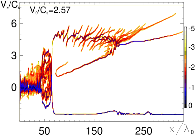
Figure 5: PIC simulation result from Ref. Liseykina15 . Shown is the ion phase plane at $t\omega_{pe}=2800$, $M_{0}=V_{0}/C_{s}=2.57$; the resulting velocity of the shock is around 3.8. The color coding corresponds to the ion phase space density normalized to that of the upstream ions (logarithmic scale).

References

- (1) R. Z. Sagdeev, Reviews of Plasma Physics 4, 23 (1966).
- (2) D. Tidman and N. Krall, Shock waves in collisionless plasmas, Wiley series in plasma physics (Wiley-Interscience, ADDRESS, 1971).
- (3) C. F. Kennel, J. P. Edmiston, and T. Hada, Washington DC American Geophysical Union Geophysical Monograph Series 34, 1 (1985).
- (4) K. Papadopoulos, Washington DC American Geophysical Union Geophysical Monograph Series 34, 59 (1985).
- (5) R. Blandford and D. Eichler, Phys. Rep. 154, 1 (1987).
- (6) M. A. Malkov and L. O. Drury, Reports on Progress in Physics 64, 429 (2001).
- (7) R. Blandford, P. Simeon, and Y. Yuan, Nuclear Physics B Proceedings Supplements 256, 9 (2014).
- (8) S. V. Bulanov et al., Physics Letters A 299, 240 (2002).
- (9) D. Haberberger et al., Nature Physics 8, 95 (2012).
- (10) F. Fiuza et al., Physics of Plasmas 20, 056304 (2013).
- (11) Y. V. Medvedev, Plasma Physics Reports 35, 62 (2009).
- (12) S. S. Moiseev and R. Z. Sagdeev, Journal of Nuclear Energy 5, 43 (1963).
- (13) A. V. Gurevich, Soviet Journal of Experimental and Theoretical Physics 26, 575 (1968).
- (14) L. D. Landau and E. M. Lifshitz, Fluid Mechanics (Pergamon Press, ADDRESS, 1987).
- (15) A. V. Gurevich and L. P. Pitaevskii, Progress in Aerospace Sciences 16, 227 (1975).
- (16) J. C. Polf and K. Parodi, Physics Today 68, 28 (2015).
- (17) G. A. Mourou, T. Tajima, and S. V. Bulanov, Reviews of Modern Physics 78, 309 (2006).
- (18) C. A. J. Palmer et al., Phys. Rev. Lett. 106, 014801 (2011).
- (19) A. Macchi, M. Borghesi, and M. Passoni, Rev. Mod. Phys. 85, 751 (2013).
- (20) M. A. Malkov and H. J. Völk, Astronomy and Astrophys.300, 605 (1995).
- (21) M. A. Malkov, Phys. Rev. E 58, 4911 (1998).
- (22) G. P. Zank et al., Physics of Plasmas 8, 4560 (2001).
- (23) O. Adriani et al., Science 332, 69 (2011).
- (24) L. Accardo et al., Physical Review Letters 113, 121101 (2014).
- (25) M. A. Malkov, P. H. Diamond, and R. Z. Sagdeev, Physical Review Letters 108, 081104 (2012).
- (26) V. S. Berezinskii, S. V. Bulanov, V. A. Dogiel, and V. S. Ptuskin, in Astrophysics of cosmic rays, edited by V. L. Ginzburg (Amsterdam: North-Holland, ADDRESS, 1990).
- (27) A. M. Hillas, Journal of Physics G Nuclear Physics 31, 95 (2005).
- (28) L. O. . Drury, Astroparticle Physics 39, 52 (2012).
- (29) T. K. Gaisser, T. Stanev, and S. Tilav, Frontiers of Physics 8, 748 (2013).
- (30) A. R. Bell, Brazilian Journal of Physics 44, 415 (2014).
- (31) H. Kucharek and M. Scholer, J. Geophys. Res. 96, 21195 (1991).
- (32) M. Scholer, H. Kucharek, and C. Kato, Physics of Plasmas 9, 4293 (2002).
- (33) D. Burgess, E. Möbius, and M. Scholer, Space Sci. Rev. 50 (2012).
- (34) F. Guo and J. Giacalone, Astrophys. J. 773, 158 (2013).
- (35) D. Caprioli, A.-R. Pop, and A. Spitkovsky, Astrophys. J. Lett. 798, L28 (2015).
- (36) L. C. Woods, Plasma Physics 13, 289 (1971).
- (37) M. Gedalin, M. Liverts, and M. A. Balikhin, Journal of Geophysical Research (Space Physics) 113, 5101 (2008).
- (38) G. P. Zank, H. L. Pauls, I. H. Cairns, and G. M. Webb, J. Geophys. Res. 101, 457 (1996).
- (39) M. A. Lee, V. D. Shapiro, and R. Z. Sagdeev, J. Geophys. Res. 101, 4777 (1996).
- (40) J. P. Edmiston, C. F. Kennel, and D. Eichler, Geophys. Res. Lett. 9, 531 (1982).
- (41) T. V. Liseykina, G. I. Dudnikova, V. A. Vshivkov, and M. A. Malkov, Journal of Plasma Physics 81, (2015).
- (42) A. Macchi et al., Plasma Physics and Controlled Fusion 55, 124020 (2013).