Lessons learnt from the Solar neighbourhood and the Kepler field

Abstract

Setting the timeline of the events which shaped the Milky Way disc through its 13 billion year old history is one of the major challenges in the theory of galaxy formation. Achieving this goal is possible using late-type stars, which in virtue of their long lifetimes can be regarded as fossil remnants from various epochs of the formation of the Galaxy. There are two main paths to reliably age-date late-type stars: astrometric distances for stars in the turn-off and subgiant region, or oscillation frequencies along the red giant branch. So far, these methods have been applied to large samples of stars in the solar neighbourhood, and in the Kepler field. I review these studies, emphasize how they complement each other, and highlight some of the constraints they provide for Galactic modelling. I conclude with the prospects and synergies that astrometric (Gaia) and asteroseismic space-borne missions reserve to the field of Galactic Archaeology, and advocate that survey selection functions should be kept as simple as possible, relying on basic observables such as colours and magnitudes only.

1 Introduction

Late-type stars (broadly FGKM) are long-lived objects and can be regarded as snapshots of the stellar populations that are formed at different times and places over the history of our Galaxy. The fundamental properties of a sizeable number of these stars in the Milky Way enable us to directly access different phases of its formation and evolution, and for obvious reasons, stars in the vicinity of the Sun have been preferred targets to this purpose, both in photometric and spectroscopic investigations (e.g., Gliese 1957; Wallerstein 1962; Twarog 1980; Strömgren 1987; Edvardsson et al. 1993; Nordström et al. 2004; Reddy et al. 2006; Casagrande et al. 2011; Haywood et al. 2013; Bensby et al. 2014). Properties of stars in the solar neighbourhood, in particular ages and metallicities, are still one of the main constraints for Galactic chemo(dynamical) models, and provide important clues to understand some of the main processes at play in galaxy formation and evolution (e.g., Matteucci & Francois 1989; Portinari et al. 1998; Chiappini et al. 2001; Roškar et al. 2008; Schönrich & Binney 2009; Just & Jahreiß 2010; Minchev et al. 2013; Bird et al. 2013; Kubryk et al. 2015).

A common feature of all past and current stellar surveys is that, while it is relatively straightforward to derive some sort of information on the chemical composition of the targets observed (and in many cases even detailed abundances), this is not always the case when it comes to stellar masses, radii, and in particular, ages. When accurate astrometric distances are available to allow comparison of stars with isochrones (assuming other parameters involved in this comparison – such as effective temperatures and metallicities – are also well determined), reliable stellar ages can be derived in restricted regions of the HR diagram, such as the turnoff and subgiant phase, where stars of different ages occupy clearly different positions (roughly FG spectral types). However, even in this favourable condition, statistical techniques are still needed to avoid biases, in particular that arising from the different evolutionary speed of stellar models that populate the same region of observed parameters (the so-called terminal-age bias, e.g., Pont & Eyer 2004; Jørgensen & Lindegren 2005; Serenelli et al. 2013).

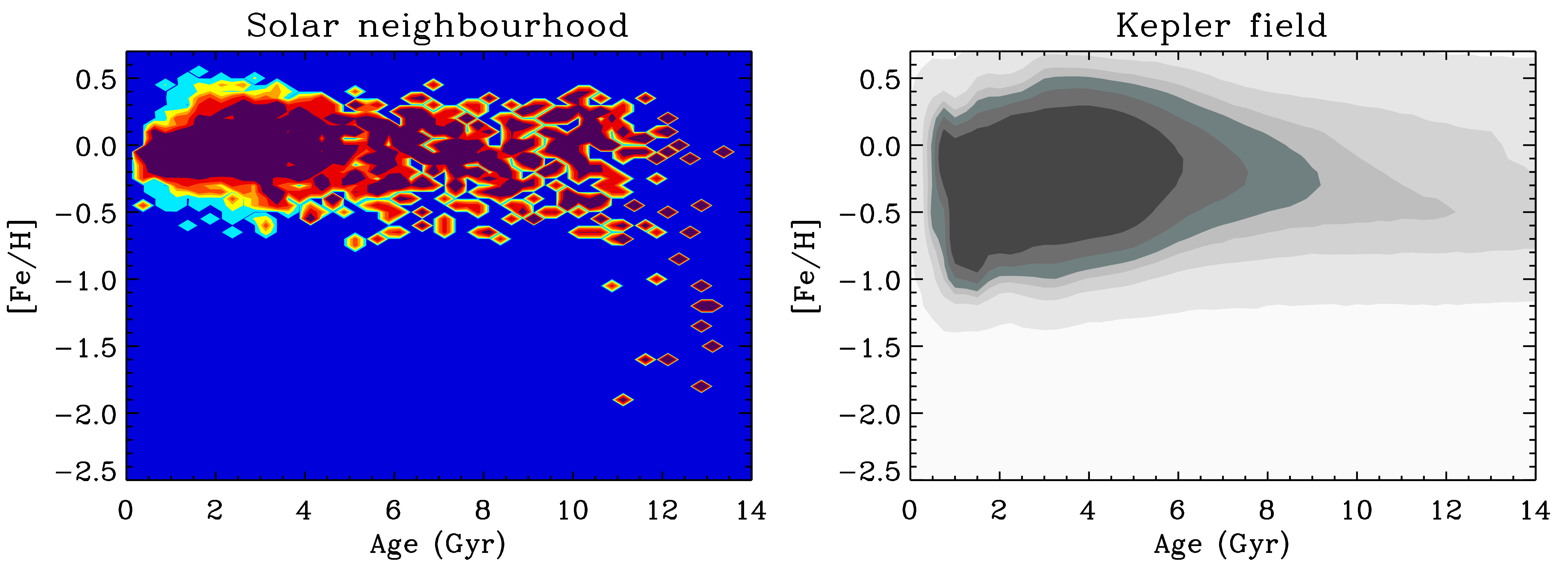
Figure 1: Left panel: age-metallicity relation from the GCS, using stars with effective temperatures determined from the InfraRed Flux Method (irfm pedigree), relative age uncertainty below 25% or absolute uncertainty below 1 Gyr (whichever is satisfied). Contours density levels are obtained using bins of $0.25$ Gyr and $0.05$ dex, to equally represent region with fewer stars. See Casagrande et al. (2011) for details. Right panel: age-metallicity relation of the Kepler field from SAGA. Contour levels have been obtained by convolving each star with its age, and metallicity uncertainties, and assigning a weight proportional to the logarithm of the inverse probability of being observed. Notice that sample selection excludes metal poor giants, thus preventing us from tracing the early chemical enrichment seen e.g. in the left hand panel. See text, and Casagrande et al. (2016) for details.

The temperature regime of late type stars is also dominated by surface convection, which is the main driver of the oscillation modes (called solar-like) that we are now able to detect in several thousands of stars thanks to space borne asteroseismic missions such as CoRoT and Kepler/K2. In particular, global oscillation frequencies not only are the easiest ones to detect and analyze, but via scaling-relations they are also linked to fundamental physical quantities such as masses and radii of stars (see e.g., Chaplin & Miglio 2013, for a review). Despite the accuracy of seismic scaling-relations has not yet been fully explored, particularly in the metal poor regime, stellar radii have been shown to be accurate to better than a few percent in dwarfs and subgiants (e.g., Huber et al. 2012; Silva Aguirre et al. 2012; White et al. 2013; Coelho et al. 2015), while masses are likely to be better than 10%, but are also less tested (Miglio et al. 2013a). More importantly, these relations are applicable to all stars displaying solar-like oscillations, i.e. also to red giants. Thus, while awaiting for more stringent tests on scaling-relations, we can already say that asteroseismology of late-type stars is able to provide stellar masses and radii to an accuracy that goes from being comparable to, to generally (much) better than achievable by isochrone fitting.

2 The Solar neighbourhood

The region of the Milky Way where we currently have the most complete chemo-dynamical inventory of stars is the Solar neighbourhood, i.e. a region of order 100 pc from us, and for which the Hipparcos satellite has measured accurate stellar distances (Perryman et al. 1997; van Leeuwen 2007). The latter, coupled with proper motions and radial velocities give the complete six-dimensional phase space information. Fundamental stellar properties, such as effective temperatures and metallicities (and even detailed elemental abundances, if possible) provide further pieces to understand the puzzle of the Milky Way’s formation.

Historically, two different approaches have been adopted to achieve this goal using stars in the Solar neighbourhood. While spectroscopic studies allow detailed abundance investigations, they have been limited to small samples of a few hundred or about a thousand stars at most, and have used sophisticated kinematic selections to sample significant numbers of members belonging to different Galactic subpopulations (e.g., Allende Prieto et al. 2004; Reddy et al. 2006; Ramírez et al. 2007; Bensby et al. 2014). Multi-object spectrographs are now changing this paradigm, but the combination of instruments’ field of view, stellar number densities, limiting magnitudes etc…makes these facilities better suited to probe pencil beams through the Galaxy. Another approach consists instead of using photometry to build large sample of stars with well defined selection criteria in observational space, typically colours and magnitudes. In turns, this implies well controlled and/or little selection biases, though at the price of not being able to derive detailed elemental abundances from photometry. See e.g., Ivezić et al. (2012) for the latest review on stellar surveys, or Casagrande (2015) for the rationale behind photometric parameters, and a brief discussion of pros and cons between photometric and spectroscopic surveys.

Arguably, the most complete census of Solar neighbourhood stars is currently provided by the Geneva-Copenhagen Survey (GCS, Nordström et al. 2004) an all-sky, shallow survey comprising over $14,000$ main-sequence and subgiant stars closer than $\simeq 100$ pc (40 pc volume limited). The GCS provides the ideal dataset for studies dealing with Galactic chemical and dynamical evolution: it is kinematically unbiased, all its stars have radial velocities, proper motions, Hipparcos parallaxes, plus highly homogeneous photometry to derive fundamental stellar parameters. Stellar parameters in the GCS have undergone a number of revisions (Holmberg et al. 2007, 2009; Casagrande et al. 2011). All results presented in the following are based on the latest one, which has improved upon stellar effective temperatures, metallicities and ages.

Given its nearly volume complete nature, the GCS is well suited for the study of the metallicity distribution function in the solar neighbourhood. The peak of this function is only slightly subsolar, thus making the Sun a rather average star given its metallicity. The metallicity distribution function has been historically used to constrain the gas infall rate (e.g., Lynden-Bell 1975), but slicing it into different age bins suggests that old stars are also a relevant ingredient in describing the wings of the metallicity distribution function. A natural explanation to this is provided by radial migration, where the solar neighbourhood is not only assembled from local stars, following a local age-metallicity relation, but also from objects originating from the inner (more metal-rich) and outer (more metal-poor) Galactic disc that have migrated to the present position on different timescales (e.g., Roškar et al. 2008; Schönrich & Binney 2009; Kubryk et al. 2015). Continuing along the same line of reasoning, it thus follows that in the presence of stellar migration, the age-metallicity relation measured locally will be flat, due to the superposition of monotonic relations expected at different Galactocentric radii (see e.g., figure 6 in Schönrich & Binney 2009). This is indeed what is seen in the GCS (Figure 1, left hand panel). As we have already pointed out, the GCS has a small spatial extent, but the stellar properties measured locally can be dynamically stretched across several kiloparsecs using kinematics. For example, the azimuthal velocities ($V$) of stars can be used to derive radial gradients across several kpc. Likewise, vertical velocities ($W$), or the velocity dispersion of stars can be use infer vertical gradients well beyond the small volume covered by the GCS (see e.g., Holmberg et al. 2007; Casagrande et al. 2011). In this context, of particular interests is the age-velocity dispersion relation, a dynamical tracer of the formation history of the disc. Its exact form has been debated over the years (e.g., Wielen 1977; Carlberg et al. 1985; Edvardsson et al. 1993; Binney et al. 2000; Holmberg et al. 2007; Casagrande et al. 2011), yet its existence clearly indicates the presence of a vertical age gradient in the disc. As we see in the next Section, asteroseismology of red giants in the Kepler field allows this to be measured quantitatively for the first time.

Figure 2: Top panel: comparison between seismic masses (Chaplin et al. 2014) and isochrone masses (Casagrande et al. 2011) for dwarf and subgiant stars in common between the GCS and the Kepler field. Open circles are the seismic results obtained when assuming an average metallicity of $-0.2$ dex for the Kepler field (see Chaplin et al. 2014, for details). Filled circles when adopting instead the proper [Fe/H] of each star. Bottom panel: same as above, but comparing seismic vs. isochrone ages. Typical error bars are shown in the upper corners.

3 The Kepler field

Asteroseismology has emerged as a powerful new tool for studying stellar populations, and the synergy between classical and asteroseismic stellar parameters is now sought by all major surveys in Galactic archaeology (e.g., Casagrande et al. 2014; Pinsonneault et al. 2014; De Silva et al. 2015; De Cat et al. 2015). Most of the stars with measured oscillations in the Kepler field are red giants, although there are more than 500 dwarfs/subgiants for which seismic radii, masses and ages have been derived (Chaplin et al. 2014). Some of these stars are also in the GCS, and a comparison between seismic parameters and those derived from isochrone fitting is shown in Figure 2. The level of agreement is reassuring, anticipating that when Gaia parallaxes will be available, isochrone dating of turn-off and subgiant stars will nicely complement with asteroseismology.

The breakthrough of asteroseismology, however, is the possibility of deriving reliable stellar ages for red giant stars, where traditional isochrone fitting fails. This is due to the fact that along the red giant branch isochrones with vastly different ages can fit observational data such as effective temperatures, metallicities, and surface gravities equally well within their errors. However, once a star has evolved into a red giant, its age is determined to good approximation by the time spent in the hydrogen burning phase, and this is predominantly a function of mass. Thus, seismic masses provide powerful age constraints. It should be noted however that in case of mass-loss, the actual mass measured by seismology will be somewhat smaller than the initial stellar mass (which sets the evolutionary timescale), and uncertainties related to mass-loss might be the main limiting factor to derive precise seismic ages for red giants. Another advantage of using red giants stems from their intrinsic luminosities, meaning that they can be easily used to probe distances up to a few kpc.

Various schemes are now being developed to derive seismic ages across the HR diagram, using different stellar models, and assessing the impact of different input physics (e.g., Silva Aguirre et al. 2013, 2015; Lebreton & Goupil 2014; Rodrigues et al. 2014). The first effort of using seismic ages for the sake of Galactic studies has been put into place with the Strömgren survey for Asteroseismology and Galactic Archaeology (SAGA), which so far has derived classical and seismic stellar parameters for giants in the Kepler field, covering Galactic latitudes from about $8^{\circ}$ to $20^{\circ}$, at a fixed Galactic longitude, implying nearly constant Galactocentric distances. This choice of geometry minimizes radial variations, and makes the sample ideal to study the vertical structure of the disc, thus allowing a direct measurement of the vertical age gradient kinematically inferred from the GCS (see previous Section). SAGA builds on the legacy of the GCS by using Strömgren photometry, although it leverages on asteroseismology. For a detailed accounting of the SAGA survey and its application to Galactic studies see Casagrande et al. (2014); Casagrande et al. (2016).

The right hand panel in Figure 1 shows the age-metallicity relation derived using red giants with seismic ages. This plot has been corrected to factor out the main biases due to the complicated Kepler selection function, as well as target selection effects. Similarly to what is seen in the solar neighbourhood, also for the Kepler field there is a rather flat age-metallicity relation. There is a somewhat larger metallicity spread, although this is likely due to the lower precision of the Strömgren [Fe/H] calibration adopted for giants in SAGA, compared to dwarfs and subgiants in the GCS. It should also be pointed out that sample selection excludes metal poor giants, thus preventing us from tracing the early chemical enrichment, well visible instead in the steep rise at $\sim 12$ Gyr for the Solar neighbourhood (left hand panel).

4 Selection functions and selection effects: preventing them, dealing with them

As we have already pointed out, despite being spatially limited, the GCS is ideal for a number of Galactic studies because of its volume complete nature. However, more often than not, this is not the case for other surveys. For example, pencil beam geometries are prone to various biases (among which a correlation between Galactic heights and distances, see e.g., Schönrich et al. 2014). In the case of the Kepler field, further biases stem from the fact that the mission was not designed for population nor Galactic studies, and thus it is not straightforward to assess whether stars with different properties have been preferentially, or not, observed.

As it is often the case, before using any sample of stars for studies dealing with Galactic structure, two questions must be answered. First, the survey selection function must the understood. In the case of Kepler it means understanding to which extent asteroseismic giants are representative of the underlying population of giants in the field. The best way of assessing this is by using a sample unbiased over a large colour and magnitude range, built e.g., from a magnitude complete photometric catalogue. More specifically, this means benchmarking the asteroseismic sample against a (photometrically) unbiased sample, to derive the colour and magnitude ranges where the asteroseismic sample can be thought as randomly drawn from the field. In the ideal case, a survey selection function should be clearly defined before observations even begin, although contingent situations (known and unknown unknowns, sic) might also play a role in modifying it. The crucial point is that a survey selection function should always be defined upon simple observables, such as colour and magnitude intervals. More generally, one can also envisage doing this in a multi-dimensional space, using different combinations of filters (see e.g., Bessell 2005; Casagrande & VandenBerg 2014, for the sensitivity of bandpasses to various parameters). Colour and magnitude intervals should be sufficiently large to minimize boundary effects, such as diffusion of stars in and out of the boundaries due to observational errors. Reddening will also play a role, and again defining sufficiently large intervals will minimize the impact of extinction-driven colour and magnitude shifts across a selection function. Also, reddening corrections should not be applied beforehand, or a selection function will depend upon our (in)ability to estimate reddening at a given time. More generally, while observations will stay unchanged, defining a selection function upon variables which are not observed (including stellar parameters) will make the selection itself subject to the unavoidable biases and inaccuracies of those variables. Further, future improvements in determining certain parameters might clutter the original selection criteria, thus making very hard –if at all possible– to have control on them. On the contrary, a clear and simple selection based on observables can always be reproduced, and future improvements in determining stellar parameters, correcting for reddening, predicting synthetic colours, etc…can always be incorporated when forward modelling observations.

Once clear selection criteria are defined, we must still quantify the probability that a star with certain stellar parameters will be observed. This is due to target selection effects, i.e. how stellar parameters affect the location of a star on the HR diagram, and thus how likely it is that a star having certain parameters will pass our colour and magnitude cuts. To assess these effects, a certain degree of modelling is needed. See e.g., Casagrande et al. (2016) for a discussion of different approaches to cope with the target selection function and target selection effects of seismic targets in the Kepler field; an excellent and more general discussion can be found in Rix & Bovy (2013).

Looking ahead, the prospects of current and future asteroseismic missions for Galactic studies are bright. To this purpose, now that CoRoT and Kepler have demonstrated the potential of using red-giants for Galactic studies (e.g., Miglio et al. 2013b; Chiappini et al. 2015; Martig et al. 2015; Casagrande et al. 2016), a better selection function has been adopted for K2 (Stello et al. 2015). The relevance of Galactic science has also surged in future space-borne missions with asteroseismic capabilities, such as TESS, PLATO and WFIRST. Much before those, Gaia astrometry will dramatically increase the volume for which we will know the full stellar phase space information, and soon make possible to derive ages for turn-off and subgiant stars across different Galactic components. The mapping and dating of our Galaxy have just begun!