Asymptotic Normality of Quadratic Estimators

Abstract

We prove conditional asymptotic normality of a class of quadratic U-statistics that are dominated by their degenerate second order part and have kernels that change with the number of observations. These statistics arise in the construction of estimators in high-dimensional semi- and non-parametric models, and in the construction of nonparametric confidence sets. This is illustrated by estimation of the integral of a square of a density or regression function, and estimation of the mean response with missing data. We show that estimators are asymptotically normal even in the case that the rate is slower than the square root of the observations.

1 Introduction

Let $(X_{1},Y_{1}),\ldots,(X_{n},Y_{n})$ be i.i.d. random vectors, taking values in sets ${\cal X}\times\mathbb{R}$, for an arbitrary measurable space $({\cal X},{\cal A})$ and $\mathbb{R}$ equipped with the Borel sets. For given symmetric, measurable functions $K_{n}:{\cal X}\times{\cal X}\to\mathbb{R}$ consider the $U$-statistics

$$U_{n}={1\over n(n-1)}\mathop{\mathchar 4944\relax\mathchar 4944\relax}\limits_{1\leq r\not=s\leq n}K_{n}(X_{r},X_{s})Y_{r}Y_{s}.$$ (1)

Would the kernel $(x_{1},y_{1},x_{2},y_{2})\mapsto K_{n}(x_{1},x_{2})y_{1}y_{2}$ of the $U$-statistic be independent of $n$ and have a finite second moment, then either the sequence $\sqrt{n}(U_{n}-\mathord{\rm E}U_{n})$ would be asymptotically normal or the sequence $n(U_{n}-\mathord{\rm E}U_{n})$ would converge in distribution to Gaussian chaos. The two cases can be described in terms of the Hoeffding decomposition $U_{n}=\mathord{\rm E}U_{n}+U_{n}^{(1)}+U_{n}^{(2)}$ of $U_{n}$, where $U_{n}^{(1)}$ is the best approximation of $U_{n}-\mathord{\rm E}U_{n}$ by a sum of the type ${\sum_{i=1}^{n}}h(X_{r},Y_{r})$ and $U_{n}^{(2)}$ is the remainder, a degenerate $U$-statistic (compare (28) in Section 5). For a fixed kernel $K_{n}$ the linear term $U_{n}^{(1)}$ dominates as soon as it is nonzero, in which case asymptotic normality pertains; in the other case $U_{n}^{(1)}=0$ and the $U$-statistic possesses a nonnormal limit distribution.

If the kernel depends on $n$, then the separation between the linear and quadratic cases blurs. In this paper we are interested in this situation and specifically in kernels $K_{n}$ that concentrate as $n\rightarrow\infty$ more and more near the diagonal of ${\cal X}\times{\cal X}$. In our situation the variance of the $U$-statistics is dominated by the quadratic term $U_{n}^{(2)}$. However, we show that the sequence $(U_{n}-\mathord{\rm E}U_{n})/{\sigma}(U_{n})$ is typically still asymptotically normal. The intuitive explanation is that the $U$-statistics behave asymptotically as “sums across the diagonal $r=s$” and thus behave as sums of independent variables. Our formal proof is based on establishing conditional asymptotic normality given a binning of the variables $X_{r}$ in a partition of the set ${\cal X}$.

Statistics of the type (1) arise in many problems of estimating a functional on a semiparametric model, with $K_{n}$ the kernel of a projection operator (see [1]). As illustrations we consider in this paper the problems of estimating $\int g^{2}(x)\,dx$ or $\int f^{2}(x)\,dG(x)$, where $g$ is a density and $f$ a regression function, and of estimating the mean treatment effect in missing data models. Rate-optimal estimators in the first of these three problems were considered by [2, 3, 4, 5, 6], among others. In Section 3 we prove asymptotic normality of the estimators in [4, 5], also in the case that the rate of convergence is slower than $\sqrt{n}$, usually considered to be the “nonnormal domain”. For the second and third problems estimators of the form (1) were derived in [1, 7, 8, 9] using the theory of second-order estimating equations. Again we show that these are asymptotically normal, also in the case that the rate is slower than $\sqrt{n}$.

Statistics of the type (1) also arise in the construction of adaptive confidence sets, as in [10], where the asymptotic normality can be used to set precise confidence limits.

Previous work on $U$-statistics with kernels that depend on $n$ includes [11, 12, 13, 14, 15]. These authors prove unconditional asymptotic normality using the martingale central limit theorem, under somewhat different conditions. Our proof uses a Lyapounov central limit theorem (with moment $2+{\varepsilon}$) combined with a conditioning argument, and an inequality for moments of $U$-statistics due to E. Giné. Our conditions relate directly to the contraction of the kernel, and can be verified for a variety of kernels. The conditional form of our limit result should be useful to separate different roles for the observations, such as for constructing preliminary estimators and for constructing estimators of functionals. Another line of research (as in as in [16]) is concerned with $U$-statistics that are well approximated by their projection on the initial part of the eigenfunction expansion. This has no relation to the present work, as here the kernels explode and the $U$-statistic is asymptotically determined by the (eigen) directions “added” to the kernel as the number of observations increases. By making special choices of kernel and variables $Y_{i}$, the statistics (1) can reduce to certain chisquare statistics, studied in [17, 18].

The paper is organized as follows. In Section 2 we state the main result of the paper, the asymptotic normality of $U$-statistics of the type (1) under general conditions on the kernels $K_{n}$. Statistical applications are given in Section 3. In Section 4 the conditions of the main theorem shown to be satisfied by a variety of popular kernels, including wavelet, spline, convolution, and Fourier kernels. The proof of the main result is given in Section 5, while proofs for Section 4 are given in an appendix.

The notation $a\lesssim b$ means $a\leq Cb$ for a constant $C$ that is fixed in the context. The notations $a_{n}\sim b_{n}$ and $a_{n}\ll b_{n}$ mean that $a_{n}/b_{n}\rightarrow 1$ and $a_{n}/b_{n}\rightarrow 0$, as $n\rightarrow\infty$. The space $L_{2}(G)$ is the set of measurable functions $f:{\cal X}\to\mathbb{R}$ that are square-integrable relative to the measure $G$ and $\|f\|_{G}$ is the corresponding norm. The product $f\times g$ of two functions is to be understood as the function $(x_{1},x_{2})\mapsto f(x_{1})g(x_{2})$, whereas the product $F\times G$ of two measures is the product measure.

2 Main result

In this section we state the main result of the paper, the asymptotic normality of the $U$-statistics (1), under general conditions on the kernels $K_{n}$ and distributions of the vectors $(X_{r},Y_{r})$. For $q>0$ let

$${\mu}(x) =\mathord{\rm E}\bigl{(}Y_{1}\mathchar 25194\relax X_{1}=x\bigr{)},$$

$${\mu}_{q}(x) =\mathord{\rm E}\bigl{(}|Y_{1}|^{q}\mathchar 25194\relax X_{1}=x\bigr{)}$$

be versions of the conditional (absolute) moments of $Y_{1}$ given $X_{1}$. For simplicity we assume that ${\mu}_{1}$ and and ${\mu}_{2}$ are uniformly bounded. The marginal distribution of $X_{1}$ is denoted by $G$.

The kernels are assumed to be measurable maps $K_{n}:{\cal X}\times{\cal X}\to\mathbb{R}$ that are symmetric in their two arguments and satisfy $\int\!\!\int K_{n}^{2}\,d(G\times G)<\infty$ for every $n$. Thus the corresponding kernel operators (with abuse of notation denoted by the same symbol)

$$K_{n}f(x)=\int f(v)K_{n}(x,v)\,dG(v),$$ (2)

are continuous, linear operators $K_{n}:L_{2}(G)\to L_{2}(G)$. We assume that their operator norms $\|K_{n}\|=\sup\{\|K_{n}f\|_{G}:\|f\|_{G}=1\}$ are uniformly bounded:

$$\sup_{n}\|K_{n}\|<\infty.$$ (3)

By the Banach-Steinhaus theorem this is certainly the case if $K_{n}f\rightarrow f$ in $L_{2}(G)$ as $n\rightarrow\infty$ for every $f\in L_{2}(G)$. The operator norms $\|K_{n}\|$ are typically much smaller than the $L_{2}(G\times G)$-norms of the kernels. The squares of the latter are typically of the same order of magnitude as the square $L_{2}(G\times G)$-norms weighted by ${\mu}_{2}\times{\mu}_{2}$, which we denote by

$$k_{n}:=\int\!\!\int K_{n}^{2}(x,y)\ ({\mu}_{2}\times{\mu}_{2})(x,y)\,d(G\times G)(x,y).$$ (4)

We consider the situation that these square weighted norms are strictly larger than $n$:

$${k_{n}\over n}\rightarrow\infty.$$ (5)

Under condition (5) the variance of the $U$-statistic (1) is dominated by the variance of the quadratic part of its Hoeffding decomposition. In contrast, if $k_{n}=n$, the linear and quadratic parts contribute variances of equal order. This case can be handled by the methods of this paper, but requires a special discussion, which we omit. The remaining case $k_{n}\ll n$ leads to asymptotically linear $U$-statistics, and is well understood.

The remaining conditions concern the concentration of the kernels $K_{n}$ to the diagonal of ${\cal X}\times{\cal X}$. We assume that there exists a sequence of finite partitions ${\cal X}=\cup_{m}{\cal X}_{n,m}$ in measurable sets such that

$${1\over k_{n}}\sum_{m}\int_{{\cal X}_{n,m}}\!\!\int_{{\cal X}_{n,m}}K_{n}^{2}\ ({\mu}_{2}\times{\mu}_{2})\,d(G\times G) \rightarrow 1,$$ (6)

$${1\over k_{n}}\max_{m}\int_{{\cal X}_{n,m}}\!\!\int_{{\cal X}_{n,m}}K_{n}^{2}\ ({\mu}_{2}\times{\mu}_{2})\,d(G\times G) \rightarrow 0,$$ (7)

$$\max_{m}G({\cal X}_{n,m}) \rightarrow 0,$$ (8)

$$\liminf_{n\rightarrow\infty}n\,\min_{m}G({\cal X}_{n,m}) >0.$$ (9)

The sum in the first condition (6) is the integral of the square kernel (weighted by the function ${\mu}_{2}\times{\mu}_{2}$) over the set $\cup_{m}({\cal X}_{n,m}\times{\cal X}_{n,m})$ (shown in Figure 1). The condition requires this to be asymptotically equivalent to the integral $k_{n}$ of this same function over the whole product space ${\cal X}\times{\cal X}$. The other conditions implicitly require that the partitioning sets are not too different and not too numerous.

Figure 1: The diagonal of ${\cal X}\times{\cal X}$ covered by the set $\cup_{m}({\cal X}_{n,m}\times{\cal X}_{n,m})$.

A final condition requires implicitly that the partitioning is fine enough. For some $q>2$, the partitions should satisfy

$$\frac{1}{k_{n}^{q/2}}\max_{m}\Bigl{(}{G({\cal X}_{n,m})\over n}\Bigr{)}^{q/2-1}\sum_{m}\int_{{\cal X}_{n,m}}\!\!\int_{{\cal X}_{n,m}}\!\!|K_{n}|^{q}({\mu}_{q}\times{\mu}_{q})\,d(G\times G)\!\rightarrow 0.$$ (10)

This condition will typically force the number of partitioning sets to infinity at a rate depending on $n$ and $k_{n}$ (see Section 4). In the proof it serves as a Lyapounov condition to enforce normality.

The existence of partitions satisfying the preceding conditions depends mostly on the kernels $K_{n}$, and is established for various kernels in Section 4. The following theorem is the main result of the paper. Its proof is deferred to Section 5.

Let $I_{n}$ be the vector with as coordinates $I_{n,1},\ldots,I_{n,n}$ the indices of the partitioning sets containing $X_{1},\ldots,X_{n}$, i.e. $I_{n,r}=m$ if $X_{r}\in{\cal X}_{n,m}$. Recall that the bounded Lipschitz distance generates the weak topology on probability measures.

Theorem 2.1.

Assume that the function ${\mu}_{2}$ is uniformly bounded. If (3) and (5) hold and there exist finite partitions ${\cal X}=\cup_{m}{\cal X}_{n,m}$ such that (6)–(10) hold, then the bounded Lipschitz distance between the conditional law of $(U_{n}-\mathord{\rm E}U_{n})/{\sigma}(U_{n})$ given $I_{n}$ and the standard normal distribution tends to zero in probability. Furthermore $\mathop{\rm var}\nolimits U_{n}\sim 2k_{n}/n^{2}$ for $k_{n}$ given in (4).

The conditional convergence in distribution implies the unconditional convergence. It expresses that the randomness in $U_{n}$ is asymptotically determined by the fine positions of the $X_{i}$ within the partitioning sets, the numbers of observations falling in the sets being fixed by $I_{n}$.

In most of our examples the kernels are pointwise bounded above by a multiple of $k_{n}$, and (4) arises, because the area where $K_{n}$ is significantly different from zero is of the order $k_{n}^{-1}$. Condition (10) can then be simplified to

$$\max_{m}G({\cal X}_{n,m})\frac{k_{n}}{n}\rightarrow 0.$$ (11)

Lemma 2.1.

Assume that the functions ${\mu}_{2}$ and ${\mu}_{q}$ are bounded away from zero and infinity, respectively. If $\|K_{n}\|_{\infty}\lesssim k_{n}$, then (10) is implied by (11).

Proof.

The sum in (10) is bounded up to a constant by $\int\int|K_{n}|^{q}\,d(G\times G)$, which is bounded above by a constant times $k_{n}^{q-2}\int\int K_{n}^{2}\,d(G\times G)\lesssim k_{n}^{q-1}$, by the definition of $k_{n}$.   

3 Statistical applications

In this section we give examples of statistical problems in which statistics of the type (1) arise as estimators.

3.1 Estimating the integral of the square of a density

Let $X_{1},\ldots,X_{n}$ be i.i.d. random variables with a density $g$ relative to a given measure ${\nu}$ on a measurable space $({\cal X},{\cal A})$. The problem of estimating the functional $\int g^{2}\,d{\nu}$ has been addressed by many authors, including [2], [6] and [19]. The estimators proposed by [4, 5], which are particularly elegant, are based on an expansion of $g$ on an orthonormal basis $e_{1},e_{2},\ldots$ of the space $L_{2}({\cal X},{\cal A},{\nu})$, so that $\int g^{2}\,d{\nu}=\sum_{i=1}^{\infty}{\theta}_{i}^{2}$, for ${\theta}_{i}=\int ge_{i}\,d{\nu}$ the Fourier coefficients of $g$. Because $\mathord{\rm E}e_{i}(X_{1})e_{i}(X_{2})={\theta}_{i}^{2}$, the square Fourier coefficient ${\theta}_{i}^{2}$ can be estimated unbiasedly by the $U$-statistic with kernel $(x_{1},x_{2})\mapsto e_{i}(x_{1})e_{i}(x_{2})$. Hence the truncated sum of squares ${\sum_{i=1}^{k}}{\theta}_{i}^{2}$ can be estimated unbiasedly by

$$U_{n}={\sum_{i=1}^{k}}{1\over n(n-1)}\mathop{\mathchar 4944\relax\mathchar 4944\relax}\limits_{r\not=s}e_{i}(X_{r})e_{i}(X_{s}).$$

This statistic is of the type (1) with kernel $K_{n}(x_{1},x_{2})={\sum_{i=1}^{k}}e_{i}(x_{1})e_{i}(x_{2})$ and the variables $Y_{1},\ldots,Y_{n}$ taken equal to unity.

The estimator $U_{n}$ is unbiased for the truncated series ${\sum_{i=1}^{k}}{\theta}_{i}^{2}$, but biased for the functional of interest $\int g^{2}\,d{\nu}=\sum_{i=1}^{\infty}{\theta}_{i}^{2}$. The variance of the estimator can be computed to be of the order $k/n^{2}\vee 1/n$ (cf. (29) below). If the Fourier coefficients are known to satisfy $\sum_{i=1}^{\infty}{\theta}_{i}^{2}i^{2{\beta}}\leq 1$, then the bias can be bounded by $\sum_{i=k+1}^{\infty}{\theta}_{i}^{2}\leq k^{-2{\beta}}$, and trading square bias versus the variance leads to the choice $k=n^{1/(2{\beta}+1/2)}$.

In the case that ${\beta}>1/4$, the mean square error of the estimator is $1/n$ and the sequence $\sqrt{n}(U_{n}-\int g^{2}\,d{\nu})$ can be shown to be asymptotically linear in the efficient influence function $2(g-\int g^{2}\,d{\nu})$ (see (28) with ${\mu}(x)=\mathord{\rm E}(Y_{1}\mathchar 25194\relax X_{1}=x)\equiv 1$ and [4], [5]). More interesting from our present perspective is the case that $0<{\beta}<1/4$, when the mean square error is of order $n^{-4{\beta}/(2{\beta}+1/2)}\gg 1/n$, and the variance of $U_{n}$ is dominated by its second-order term. By Theorem 2.1 the estimator, centered at its expectation, and with the orthonormal basis $(e_{i})$ one of the bases discussed in Section 4, is still asymptotically normally distributed.

3.2 Estimating the integral of the square of a regression function

Let $(X_{1},Y_{1}),\ldots,(X_{n},Y_{n})$ be i.i.d. random vectors following the regression model $Y_{i}=b(X_{i})+{\varepsilon}_{i}$ for unobservable errors ${\varepsilon}_{i}$ that satisfy $\mathord{\rm E}({\varepsilon}_{i}\mathchar 25194\relax X_{i})=0$. It is desired to estimate $\int b^{2}\,dG$ for $G$ the marginal distribution of $X_{1},\ldots,X_{n}$.

If the distribution $G$ is known, then an appropriate estimator can take exactly the form (1), for $K_{n}$ the kernel of an orthonormal projection on a suitable $k_{n}$-dimensional space in $L_{2}(G)$. Its asymptotics are as in Section 3.1.

Because an orthogonal projection in $L_{2}(G)$ can only be constructed if $G$ is known, the preceding estimator is not available if $G$ is unknown. If the regression function $b$ is regular of order ${\beta}\geq 1/4$, then the parameter can be estimated at $\sqrt{n}$-rate (see [1]). In this section we consider an estimator that is appropriate if $b$ is regular of order ${\beta}<1/4$ and the design distribution $G$ permits a Lebesgue density $g$ that is bounded away from zero and sufficiently smooth.

Given initial estimators $\hat{b}_{n}$ and $\hat{g}_{n}$ for the regression function $b$ and design density $g$, we consider the estimator

$$T_{n} ={1\over n}\sum_{r=1}^{n}\Bigl{(}\hat{b}_{n}(X_{r})^{2}+2\hat{b}_{n}(X_{r})\bigl{(}Y_{r}-\hat{b}_{n}(X_{r})\bigr{)}\Bigr{)}$$

$$\qquad+{1\over n(n-1)}\mathop{\mathchar 4944\relax\mathchar 4944\relax}\limits_{1\leq r\not=s\leq n}\bigl{(}Y_{r}-\hat{b}_{n}(X_{r})\bigr{)}K_{k_{n},\hat{g}_{n}}(X_{r},X_{s})\bigl{(}Y_{s}-\hat{b}_{n}(X_{s})\bigr{)}.$$ (12)

Here $(x_{1},x_{2})\mapsto K_{k,g}(x_{1},x_{2})$ is a projection kernel in the space $L_{2}(G)$. For definiteness we construct this in the form (14), where the basis $e_{1},\ldots,e_{k}$ may be the Haar basis, or a general wavelet basis, as discussed in Section 4. Alternatively, we could use projections on the Fourier or spline basis, or convolution kernels, but the latter two require twicing (see (16)) to control bias, and the arguments given below must be adapted.

The initial estimators $\hat{b}_{n}$ and $\hat{g}_{n}$ may be fairly arbitrary rate-optimal estimators if constructed from an independent sample of observations. (e.g. after splitting the original sample in parts used to construct the initial estimators and the estimator (12)). We assume this in the following theorem, and also assume that the norm of $\hat{b}_{n}$ in $C^{\beta}[0,1]$ is bounded in probability, or alternatively, if the projection is on the Haar basis, that this estimator is in the linear span of $e_{1},\ldots,e_{k_{n}}$. This is typically not a loss of generality.

Let $\hat{\mathord{\rm E}}$ and $\hat{\mathop{\rm var}\nolimits}$ denote expectation and variance given the additional observations. Set ${\mu}_{q}(x)=\mathord{\rm E}(|{\varepsilon}_{1}|^{q}\mathchar 25194\relax X_{1}=x)$ and let $\|\cdot\|_{3}$ denote the $L_{3}$-norm relative to Lebesgue measure.

Corollary 3.1.

Let $\hat{b}_{n}$ and $\hat{g}_{n}$ be estimators based on independent observations that converge to $b$ and $g$ in probability relative to the uniform norm and satisfy $\|\hat{b}_{n}-b\|_{3}=O_{P}(n^{-{\beta}/(2{\beta}+1)})$ and $\|\hat{g}_{n}-g\|_{3}=O_{P}(n^{-{\gamma}/(2{\gamma}+1)})$. Let ${\mu}_{q}$ be finite and uniformly bounded for some $q>2$. Then for $b\in C^{\beta}[0,1]$ and strictly positive $g\in C^{\gamma}[0,1]$, with ${\gamma}\geq{\beta}$, and for $k_{n}$ satisfying (5),

$$\Bigl{|}\hat{\mathord{\rm E}}_{b,g}T_{n}-\int b^{2}dG\Bigr{|} =O_{P}\Bigl{(}{1\over k_{n}}\Bigr{)}^{2{\beta}}+O_{P}\Bigl{(}{1\over n}\Bigr{)}^{2{\beta}/(2{\beta}+1)+{\gamma}/(2{\gamma}+1)},$$

$$\hat{\mathop{\rm var}\nolimits}_{b,g}T_{n} ={2\over n^{2}}\int\!\!\int({\mu}_{2}\times{\mu}_{2})K_{k_{n},g}^{2}\,d(G\times G)\bigl{(}1+o_{P}(1)\bigr{)}=O_{P}\Bigl{(}{k_{n}\over n^{2}}\Bigr{)}.$$

Furthermore, the sequence $(T_{n}-\hat{\mathord{\rm E}}_{b,g}T_{n})/\hat{\mathop{\rm sd}\nolimits}_{b,g}(T_{n})$ tends in distribution to the standard normal distribution.

For $k_{n}=n^{1/(2{\beta}+1/2)}$ the estimator $T_{n}$ of $\int b^{2}\,dG$ attains a rate of convergence of the order $n^{-2{\beta}/(2{\beta}+1/2)}+n^{-2{\beta}/(2{\beta}+1)-{\gamma}/(2{\gamma}+1)}$. If ${\gamma}>{\beta}/(4{\beta}^{2}+{\beta}+1/2)$, then this reduces to $n^{-4{\beta}/(1+4{\beta})}$, which is known to be the minimax rate when $g$ is known and $b$ ranges over a ball in $C^{\beta}[0,1]$, for ${\beta}\leq 1/4$ (see [3] or [20]). For smaller values of ${\gamma}$ the estimator can be improved by considering third or higher order $U$-statistics (see [9]).

3.3 Estimating the mean response with missing data

Suppose that a typical observation is distributed as $X=(YA,A,Z)$ for $Y$ and $A$ taking values in the two-point set $\{0,1\}$ and conditionally independent given $Z$, with conditional mean functions $b(z)=\mathord{\rm P}(Y=1\mathchar 25194\relax Z=z)$ and $a(z)^{-1}=\mathord{\rm P}(A=1\mathchar 25194\relax Z=z)$, and $Z$ possessing density $g$ relative to some dominated measure ${\nu}$.

In [7] we introduced a quadratic estimator for the mean response $\mathord{\rm E}Y=\int bg\,d{\nu}$, which attains a better rate of convergence than the conventional linear estimators. For initial estimators $\hat{a}_{n}$, $\hat{b}_{n}$ and $\hat{g}_{n}$, and $K_{k,\hat{\alpha}_{n},\hat{g}_{n}}$ a projection kernel in $L_{2}(g/a)$, this takes the form

$$\frac{1}{n}\sum_{r=1}^{n}\Bigl{(}A_{r}\hat{a}_{n}(Z_{r})\bigl{(}Y_{r}-\hat{b}_{n}(Z_{r})\bigr{)}+\hat{b}_{n}(Z_{r}\Bigr{)}$$

$$\quad-\frac{1}{n(n-1)}\mathop{\mathchar 4944\relax\mathchar 4944\relax}\limits_{1\leq r\not=s\leq n}\Bigl{(}A_{r}\bigl{(}Y_{r}-\hat{b}_{n}(Z_{r})\bigr{)}K_{k_{n},\hat{\alpha}_{n},\hat{g}_{n}}(Z_{r},Z_{s})\bigl{(}A_{s}\hat{a}_{n}(Z_{s})-1\bigr{)}\Bigr{)}.$$

Apart from the (inessential) asymmetry of the kernel, the quadratic part has the form (1). Just as in the preceding section, the estimator can be shown to be asymptotically normal with the help of Theorem 2.1.

4 Kernels

In this section we discuss examples of kernels that satisfy the conditions of our main result. Detailed proofs are given in an appendix.

Most of the examples are kernels of projections $K$, which are characterised by the identity $Kf=f$, for every $f$ in their range space. For a projection given by a kernel, the latter is equivalent to $f(x)=\int f(v)K(x,v)\,dG(v)$ for (almost) every $x$, which suggests that the measure $v\mapsto K(x,v)\,dG(v)$ acts on $f$ as a Dirac kernel located at $x$. Intuitively, if the projection spaces increase to the full space, so that the identity is true for more and more $f$, then the kernels $(x,v)\mapsto K(x,v)$ must be increasingly dominated by their values near the diagonal, thus meeting the main condition of Theorem 2.1.

For a given orthonormal basis $e_{1},e_{2},\ldots$ of $L_{2}(G)$, the orthogonal projection onto $\mathop{\rm lin\,}\nolimits(e_{1},\ldots,e_{k})$ is the kernel operator $K_{k}:L_{2}(G)\to L_{2}(G)$ with kernel

$$K_{k}(x_{1},x_{2})={\sum_{i=1}^{k}}e_{i}(x_{1})e_{i}(x_{2}).$$ (13)

It can be checked that it has operator norm 1, while the square $L_{2}$-norm $\int\int K_{k}^{2}\,d(G\times G)=k$ of the kernel is $k$.

A given orthonormal basis $e_{1},e_{2},\ldots$ relative to a given dominating measure, can be turned into an orthonormal basis $e_{1}/\sqrt{g},e_{2}/\sqrt{g},\ldots$ of $L_{2}(G)$, for $g$ a density of $G$. The kernel of the orthogonal projection in $L_{2}(G)$ onto $\mathop{\rm lin\,}\nolimits(e_{1}/\sqrt{g},\ldots,e_{k}/\sqrt{g})$ is

$$K_{k,g}(x_{1},x_{2})={{\sum_{i=1}^{k}}e_{i}(x_{1})e_{i}(x_{2})\over\sqrt{g(x_{1})}\sqrt{g(x_{2})}}.$$ (14)

If $g$ is bounded away from zero and infinity, the conditions of Theorem 2.1 will hold for this kernel as soon as they hold for the kernel (13) relative to the dominating measure.

The orthogonal projection in $L_{2}(G)$ onto the linear span $\mathop{\rm lin\,}\nolimits(f_{1},\ldots,f_{k})$ of an arbitrary set of functions $f_{i}$ possesses the kernel

$$K_{k}(x_{1},x_{2})={\sum_{i=1}^{k}}{\sum_{j=1}^{k}}A_{i,j}f_{i}(x_{1})f_{j}(x_{2}),$$ (15)

for $A$ the inverse of the $(k\times k)$-matrix with $(i,j)$-element $\langle f_{i},f_{j}\rangle_{G}$. In statistical applications this projection has the advantage that it projects onto a space that does not depend on the (unknown) measure $G$. For the verification of the conditions of Theorem 2.1 it is useful to note that the matrix $A$ is well-behaved if $f_{1},\ldots,f_{k}$ are orthonormal relative to a measure $G_{0}$ that is not too different from $G$: from the identity ${\alpha}^{T}\bigl{(}\langle f_{i},f_{j}\rangle_{G}\bigr{)}{\alpha}=\int({\sum_{i=1}^{k}}{\alpha}_{i}f_{i})^{2}\,dG$, one can verify that the eigenvalues of $A$ are bounded away from zero and infinity if $G$ and $G_{0}$ are absolutely continuous with a density that is bounded away from zero and infinity.

Orthogonal projections $K$ have the important property of making the inner product $\langle(I-K)f,f\rangle_{G}=\|(I-K)f\|_{G}^{2}$ quadratic in the approximation error. Nonorthogonal projections, such as the convolution kernels or spline kernels discussed below, lack this property, and may result in a large bias of an estimator. Twicing kernels, discussed in [21] as a means to control the bias of plug-in estimators, remedy this problem. The idea is to use the operator $K+K^{*}-KK^{*}$, where $K^{*}$ is the adjoint of $K:L_{2}(G)\to L_{2}(G)$, instead of the original operator $K$. Because $I-K-K^{*}+KK^{*}=(I-K)(I-K^{*})$, it follows that

$$\bigl{\langle}(I-K-K^{*}+KK^{*})f,f\bigr{\rangle}_{G}=\bigr{\langle}(I-K)f,(I-K)f\bigr{\rangle}_{G}=\bigr{\|}(I-K)f\bigr{\|}^{2}_{G}.$$

If $K$ is an orthogonal projection, then $K=K^{*}$ and the twicing kernel is $K+K^{*}-KK^{*}=K$, and nothing changes, but in general using a twicing kernel can cut a bias significantly.

If $K$ is a kernel operator with kernel $(x_{1},x_{2})\mapsto K(x_{1},x_{2})$, then the adjoint operator is a kernel operator with kernel $(x_{1},x_{2})\mapsto K(x_{2},x_{1})$, and the twicing operator $K+K^{*}-KK^{*}$ is a kernel operator with kernel (which depends on $G$)

$$(x_{1},x_{2})\mapsto K(x_{1},x_{2})+K(x_{2},x_{1})-\int K(x_{1},z)K(x_{2},z)\,dG(z).$$ (16)

4.1 Wavelets

Consider expansions of functions $f\in L_{2}(\mathbb{R}^{d})$ on an orthonormal basis of compactly supported, bounded wavelets of the form

$$f(x)=\sum_{j\in\mathbb{Z}^{d}}\sum_{v\in\{0,1\}^{d}}\!\langle f,\psi_{0,j}^{v}\rangle\psi_{0,j}^{v}(x)+\sum_{i=0}^{\infty}\sum_{j\in\mathbb{Z}^{d}}\sum_{v\in\{0,1\}^{d}-\{0\}}\!\!\langle f,\psi_{i,j}^{v}\rangle\psi_{i,j}^{v}(x),$$ (17)

where the base functions $\psi_{i,j}^{v}$ are orthogonal for different indices $(i,j,v)$ and are scaled and translated versions of the $2^{d}$ base functions $\psi_{0,0}^{v}$:

$$\psi_{i,j}^{v}(x)=2^{id/2}\psi_{0,0}^{v}(2^{i}x-j).$$

Such a higher-dimensional wavelet basis can be obtained as tensor products $\psi_{0,0}^{v}=\phi^{v_{1}}\times\cdots\times\phi^{v_{d}}$ of a given father wavelet $\phi^{0}$ and and mother wavelet $\phi^{1}$ in one dimension. See for instance Chapter 8 of [22].

We shall be interested in functions $f$ with support ${\cal X}=[0,1]^{d}$. In view of the compact support of the wavelets, for each resolution level $i$ and vector $v$ only to the order $2^{id}$ base elements $\psi_{i,j}^{v}$ are nonzero on ${\cal X}$; denote the corresponding set of indices $j$ by $J_{i}$. Truncating the expansion at the level of resolution $i=I$ then gives an orthogonal projection on a subspace of dimension $k$ of the order $2^{Id}$. The corresponding kernel is

$$K_{k}(x_{1},x_{2}) =\sum_{j\in J_{0}}\sum_{v\in\{0,1\}^{d}}\!\psi_{0,j}^{v}(x_{1})\psi_{0,j}^{v}(x_{2})$$ (18)

$$\hskip 40.00006pt+\sum_{i=0}^{I}\sum_{j\in J_{i}}\sum_{v\in\{0,1\}^{d}-\{0\}}\!\!\psi_{i,j}^{v}(x_{1})\psi_{i,j}^{v}(x_{1}).$$

Proposition 4.1.

For the wavelet kernel (18) with $k=k_{n}=2^{Id}$ satisfying $k_{n}/n\rightarrow\infty$ and $k_{n}/n^{2}\rightarrow 0$ conditions (3), (6), (7), (8), (9) and (10) are satisfied for any measure $G$ on $[0,1]^{d}$ with a Lebesgue density that is bounded and bounded away from zero and regression functions ${\mu}_{2}$ and ${\mu}_{q}$ (for some $q>2$) that are bounded and bounded away from zero.

4.2 Fourier basis

Any function $f\in L_{2}[-\pi,\pi]$ can be represented through the Fourier series $f=\sum_{j\in\mathbb{Z}}f_{j}e_{j}$, for the functions $e_{j}(x)=e^{ijx}/\sqrt{2\pi}$ and the Fourier coefficients $f_{j}=\int_{-\pi}^{\pi}fe_{j}\,d{\lambda}$. The truncated series $f_{k}=\sum_{|j|\leq k}f_{j}e_{j}$ gives the orthogonal projection of $f$ onto the linear span of the function $\{e_{j}:|j|\leq k\}$, and can be written as $K_{k}f$ for $K_{k}$ the kernel operator with kernel (known as the Dirichlet kernel)

$$K_{k}(x_{1},x_{2})=\sum_{|j|\leq k}e_{j}(x_{1})e_{j}(x_{2})={\sin\bigl{(}(k+{\textstyle{\frac{1}{2}}})(x_{1}-x_{2})\bigr{)}\over 2\pi\sin\bigl{(}{\textstyle{\frac{1}{2}}}(x_{1}-x_{2})\bigr{)}}.$$ (19)

Proposition 4.2.

For the Fourier kernel (19) with $k=k_{n}$ satisfying $n\ll k_{n}\ll n^{2}$ conditions (3), (6)–(10) are satisfied for any measure $G$ on $\mathbb{R}$ with a bounded Lebesgue density and regression functions ${\mu}_{2}$ and ${\mu}_{q}$ (for some $q>2$) that are bounded and bounded away from zero.

4.3 Convolution

For a uniformly bounded function $\phi:\mathbb{R}\to\mathbb{R}$ with $\int|\phi|\,d{\lambda}<\infty$, and a positive number ${\sigma}$, set

$$K_{\sigma}(x_{1},x_{2})={1\over{\sigma}}\phi\Bigl{(}{x_{1}-x_{2}\over{\sigma}}\Bigr{)}:=\phi_{\sigma}(x_{1}-x_{2}).$$ (20)

For ${\sigma}\downarrow 0$ these kernels tend to the diagonal, with square norm of the order ${\sigma}^{-1}$.

Proposition 4.3.

For the convolution kernel (20) with ${\sigma}={\sigma}_{n}$ satisfying $n^{-2}\ll{\sigma}_{n}\ll n^{-1}$ conditions (3), (6)–(10) are satisfied for any measure $G$ on $[0,1]$ with a Lebesgue density that is bounded and bounded away from zero and regression functions ${\mu}_{2}$ and ${\mu}_{q}$ (for some $q>2$) that are bounded and bounded away from zero.

4.4 Splines

The Schoenberg space $S_{r}(T,d)$ of order $r$ for a given knot sequence $T:t_{0}=0<t_{1}<t_{2}<\cdots<t_{l}<1=t_{l+1}$ and vector of defects $d=(d_{1},\ldots,d_{l})\in\{0,\ldots,r-1\}$ are the functions $f:[0,1]\rightarrow\mathbb{R}$ whose restriction to each subinterval $(t_{i},t_{i+1})$ is a polynomial of degree $r-1$ and which are $r-1-d_{i}$ times continuously differentiable in a neighbourhood of each $t_{i}$. (Here “0 times continuously differentiable” means “continuous” and “-1 times continuously differentiable” means no restriction.) The Schoenberg space is a $k=r+\sum_{i}d_{i}$-dimensional vector space. Each “augmented knot sequence”

$$-t_{r+1}\leq\cdots\leq t_{0}=0<t_{1}<t_{2}<\cdots<t_{l}<1=t_{l+1}\leq\cdots\leq t_{l+r}$$ (21)

defines a basis $N_{1},\ldots,N_{k}$ of B-splines. These are nonnegative splines with $\sum_{j}N_{j}=1$ such that $N_{j}$ vanishes outside the interval $(t_{j}^{\prime},t_{j+r}^{\prime})$. Here the “basic knots” $(t_{j}^{\prime})$ are defined as the knot sequence $(t_{j})$, but with each $t_{i}\in(0,1)$ repeated $d_{i}$ times. See [23], pages 137, 140 and 145). We assume that $|t_{i-1}-t_{i}|\leq|t_{-1}-t_{0}|$ if $i<0$ and $|t_{i+1}-t_{i}|\leq|t_{l+1}-t_{l}|$ if $i>l$.

The quasi-interpolant operator is a projection $K_{k}:L_{1}[0,1]\to S_{r}(T,d)$ with the properties

$$\|f-K_{k}f\|_{p} \leq C_{r}\|f-S_{r}(T,d)\|_{p},$$

$$\|K_{k}f\|_{p} \leq C_{r}\|f\|_{p}.$$

for every $1\leq p\leq\infty$ and a constant $C_{r}$ depending on $r$ only (see [23], pages 144–147). It follows that the projection $K_{k}$ inherits the good approximation properties of spline functions, relative to any $L_{p}$-norm. In particular, it gives good approximation to smooth functions.

The quasi-interpolant operator $K_{k}$ is a projection onto $S_{r}(T,d)$ (i.e. $K_{k}^{2}=K_{k}$ and $K_{k}f=f$ for $f\in S_{r}(T,d)$), but not an orthogonal projection. Because the B-splines form a basis for $S_{r}(T,d)$, the operator can be written in the form $K_{k}f=\sum_{j}c_{j}(f)N_{j}$ for certain linear functionals $c_{j}:L_{1}[0,1]\to\mathbb{R}$. It can be shown that, for any $1\leq p\leq\infty$,

$$|c_{j}(f)|\leq C_{r}{1\over(t_{j+r}^{\prime}-t_{j}^{\prime})^{1/p}}\|f1_{[t_{j}^{\prime},t_{j+r}^{\prime}]}\|_{p}.$$ (22)

([23], page 145.) In particular, the functionals $c_{j}$ belong to the dual space of $L_{1}[0,1]$ and can be written as $c_{j}(f)=\int fc_{j}\,d{\lambda}$ for (with abuse of notation) certain functions $c_{j}\in L_{\infty}[0,1]$. This yields the representation of $K_{k}$ as a kernel operator with kernel

$$K_{k}(x_{1},x_{2})={\sum_{j=1}^{k}}N_{j}(x_{1})c_{j}(x_{2}).$$ (23)

Proposition 4.4.

Consider a sequence (indexed by $l$) of augmented knot sequences (21) with $l^{-1}\lesssim t_{i+1}^{l}-t_{i}^{l}\lesssim l^{-1}$ for every $0\leq i\leq l$ and splines with fixed defects $d_{i}=d$. For the corresponding (symmetrized) spline kernel (23) with $l=l_{n}$ conditions (3), (6), (7), (8), (9) and (10) are satisfied if $l_{n}/n\rightarrow\infty$ and $l_{n}/n^{2}\rightarrow 0$ for any measure $G$ on $[0,1]$ with a Lebesgue density that is bounded and bounded away from zero and regression functions ${\mu}_{2}$ and ${\mu}_{q}$ (for some $q>2$) that are bounded and bounded away from zero.

5 Proof of Theorem 2.1

For $M_{n}$ the cardinality of the partition ${\cal X}=\cup_{m}{\cal X}_{n,m}$, let $N_{n,1},\ldots,N_{n,M_{n}}$ be the numbers of $X_{r}$ falling in the partitioning sets, i.e.

$$I_{n,r} =m\quad\hbox{ if }X_{r}\in{\cal X}_{n,m},$$

$$N_{n,m} =\#(1\leq r\leq n:I_{n,r}=m).$$

The vector $N_{n}=(N_{n,1},\ldots,N_{n,M_{n}})$ is multinomially distributed with parameters $n$ and vector of success probabilities $p_{n}=(p_{n,1},\ldots,p_{n,M_{n}})$ given by

$$p_{n,m}=G({\cal X}_{n,m}).$$

Given the vector $I_{n}=(I_{n,1},\ldots,I_{n,n})$ the vectors $(X_{1},Y_{1}),\ldots,(X_{n},Y_{n})$ are independent with distributions determined by

$$X_{r} G_{n,I_{n,r}} dG_{n,I_{n,r}}=1_{{\cal X}_{n,I_{n,r}}}\,dG/p_{n,I_{n,r}}$$ has distribution given by (24)

$$Y_{r} X_{r}$$ has the same conditional distribution given as before. (25)

We define $U$-statistics $V_{n}$ by restricting the kernel $K_{n}$ to the set $\cup_{m}{\cal X}_{n,m}\times{\cal X}_{n,m}$, as follows:

$$V_{n}={1\over n(n-1)}\mathop{\mathchar 4944\relax\mathchar 4944\relax}\limits_{1\leq r\not=s\leq n}K_{n}(X_{r},X_{s})Y_{r}Y_{s}1_{(X_{r},X_{s})\in\cup_{m}{\cal X}_{n,m}\times{\cal X}_{n,m}}.$$ (26)

The proof of Theorem 2.1 consists of three elements. We show that the difference between $U_{n}$ and $V_{n}$ is asymptotically negligible due to the fact that the kernels shrink to the diagonal, we show that the statistics $V_{n}$ are conditionally asymptotically normal given the vector of bin indicators $I_{n}$, and we show that the conditional and unconditional means and variances of $V_{n}$ are asymptotically equivalent. These three elements are expressed in the following four lemmas, which should be understood all implicitly to assume the conditions of Theorem 2.1.

Lemma 5.1.

$\mathop{\rm var}\nolimits(U_{n}-V_{n})/\mathop{\rm var}\nolimits U_{n}\rightarrow 0$.

Lemma 5.2.

$\sup_{x}\bigl{|}\mathord{\rm P}(\bigl{(}V_{n}-\mathord{\rm E}(V_{n}\mathchar 25194\relax I_{n})\bigr{)}/\mathop{\rm sd}\nolimits(V_{n}\mathchar 25194\relax I_{n})\leq x\mathchar 25194\relax I_{n}\bigr{)}-\Phi(x)\bigr{|}\ {\mathchoice{\raise-1.5pt\hbox{$\buildrel\small P\over{\rightarrow}$}}{\raise-2.0pt\hbox{$\buildrel\small P\over{\rightarrow}$}}{}{}}\ 0$.

Lemma 5.3.

$\bigl{(}\mathord{\rm E}V_{n}-\mathord{\rm E}(V_{n}\mathchar 25194\relax I_{n})\bigr{)}/\mathop{\rm sd}\nolimits V_{n}\ {\mathchoice{\raise-1.5pt\hbox{$\buildrel\small P\over{\rightarrow}$}}{\raise-2.0pt\hbox{$\buildrel\small P\over{\rightarrow}$}}{}{}}\ 0$.

Lemma 5.4.

$\mathop{\rm var}\nolimits(V_{n}\mathchar 25194\relax I_{n})/\mathop{\rm var}\nolimits V_{n}\ {\mathchoice{\raise-1.5pt\hbox{$\buildrel\small P\over{\rightarrow}$}}{\raise-2.0pt\hbox{$\buildrel\small P\over{\rightarrow}$}}{}{}}\ 1$.

5.1 Proof of Theorem 2.1

By Lemmas 5.1 and 5.3 the sequence $\bigl{(}(U_{n}-\mathord{\rm E}U_{n})-(V_{n}-\mathord{\rm E}(V_{n}\mathchar 25194\relax I_{n})\bigr{)}/\mathop{\rm sd}\nolimits V_{n}$ tends to zero in probability. Because conditional and unconditional convergence in probability to a constant is the same, we see that it suffices to show that $(V_{n}-\mathord{\rm E}(V_{n}\mathchar 25194\relax I_{n})\bigr{)}/\mathop{\rm sd}\nolimits V_{n}$ converges conditionally given $I_{n}$ to the normal distribution, in probability. This follows from Lemmas 5.4 and 5.2.

The variance of $U_{n}$ is computed in (29) in Section 5.2. By the Cauchy-Schwarz inequality (cf. (2)),

$$\langle K_{n}{\mu},{\mu}\rangle_{G}^{2} \leq\|K_{n}{\mu}\|_{G}^{2}\|{\mu}\|_{G}^{2}\leq\|K_{n}\|^{2}\|{\mu}\|_{G}^{4},$$

$$\|(K_{n}{\mu})\sqrt{{\mu}_{2}}\|_{G}^{2} \leq\|{\mu}_{2}\|_{\infty}\|K_{n}{\mu}\|_{G}^{2}\leq\|{\mu}_{2}\|_{\infty}\|K_{n}\|^{2}\|{\mu}\|_{G}^{2}.$$

Because ${\mu}_{2}$ is bounded by assumption and the norms $\|K_{n}\|$ are bounded in $n$ by assumption (3), the right sides are bounded in $n$. In view of (5) it follows that the first two terms in the final expression for the variance are of lower order than the third, whence

$$\mathop{\rm var}\nolimits U_{n}\sim{2k_{n}\over n^{2}}.$$ (27)

5.2 Moments of $U$-statistics

To compute or estimate moments of $U_{n}$ we employ the Hoeffding decomposition (e.g. [24], Sections 11.4 and 12.1) $U_{n}=\mathord{\rm E}U_{n}+U_{n}^{(1)}+U_{n}^{(2)}$ of $U_{n}$ given by

$$U_{n}^{(1)} ={2\over n}\sum_{r=1}^{n}\bigl{(}K_{n}{\mu}(X_{r})Y_{r}-\mathord{\rm E}U_{n}\bigr{)},$$ (28)

$$U_{n}^{(2)} =\textstyle{1\over n(n-1)}\mathop{\mathchar 4944\relax\mathchar 4944\relax}\limits_{1\leq r\not=s\leq n}\Bigl{[}K_{n}(X_{r},X_{s})Y_{r}Y_{s}-K_{n}{\mu}(X_{r})Y_{r}-K_{n}{\mu}(X_{s})Y_{s}+\mathord{\rm E}U_{n}\Bigr{]}.$$

The variables $U_{n}^{(1)}$ and $U_{n}^{(2)}$ are uncorrelated, and so are all the variables in the single and double sums defining $U_{n}^{(1)}$ and $U_{n}^{(2)}$. It follows that

$$\mathop{\rm var}\nolimits U_{n} ={4\over n}\mathop{\rm var}\nolimits\bigl{(}K_{n}{\mu}(X_{1})Y_{1}\bigr{)}$$ (29)

$$\quad+{2\over n(n-1)}\mathop{\rm var}\nolimits\bigl{(}K_{n}(X_{1},X_{2})Y_{1}Y_{2}-K_{n}{\mu}(X_{1})Y_{1}-K_{n}{\mu}(X_{2})Y_{2}\bigr{)}$$

$$=\Bigl{[}{4\over n}-{4\over n(n-1)}\Bigr{]}\mathop{\rm var}\nolimits\bigl{(}K_{n}{\mu}(X_{1})Y_{1}\bigr{)}+{2\over n(n-1)}\!\mathop{\rm var}\nolimits\bigl{(}K_{n}(X_{1},X_{2})Y_{1}Y_{2}\bigr{)}$$

$$={4(n-2)\over n(n-1)}\|(K_{n}{\mu})\sqrt{{\mu}_{2}}\|_{G}^{2}-{4(n-2)+2\over n(n-1)}\langle K_{n}{\mu},{\mu}\rangle_{G}^{2}+{2k_{n}\over n(n-1)}$$

See equation (4) for the definition of $k_{n}$.

There is no similarly simple expression for higher moments of a $U$-statistic, but the following useful bound is (essentially) established in [25].

Lemma 5.5 (Giné, Latala, Zinn).

For any $q\geq 2$ there exists a constant $C_{q}$ such that for any i.i.d. random variables $X_{1},\ldots,X_{n}$ and degenerate symmetric kernel $K$,

$$\mathord{\rm E}\Bigl{|}{1\over n(n-1)}\mathop{\mathchar 4944\relax\mathchar 4944\relax}\limits_{1\leq r\not=s\leq n}K(X_{r},X_{s})\Bigr{|}^{q}$$

$$\qquad\leq C_{q}n^{-q}\,\Bigl{(}\mathord{\rm E}K^{2}(X_{1},X_{2})\Bigr{)}^{q/2}\vee n^{-3q/2+1}\,\mathord{\rm E}|K(X_{1},X_{2})|^{q}$$

$$\qquad\leq C_{q}n^{-q}\,\mathord{\rm E}|K(X_{1},X_{2})|^{q}.$$

Proof.

The second inequality is immediate from the fact that the $L_{2}$-norm is bounded above by the $L_{q}$-norm, and $3q/2-1\geq q$, for $q\geq 2$. For the first inequality we use (3.3) in [25] (and decoupling as explained in Section 2.5 of that paper) to see that the left side of the lemma is bounded above by a multiple of

$$n^{-q}\,\Bigl{(}\mathord{\rm E}K^{2}(X_{1},X_{2})\Bigr{)}^{q/2}\vee n^{-3q/2+1}\,\mathord{\rm E}\bigl{(}\mathord{\rm E}(K^{2}(X_{1},X_{2})\mathchar 25194\relax X_{2})\bigr{)}^{q/2}$$

$$\hskip 40.00006pt\hskip 40.00006pt\hskip 40.00006pt\hskip 40.00006pt\vee n^{2-2q}\,\mathord{\rm E}|K(X_{1},X_{2})|^{q}.$$

Because $L_{q}$-norms are increasing in $q$, the second term on the right is bounded above by $n^{-3q/2+1}\mathord{\rm E}|K(X_{1},X_{2})|^{q}$, which is also a bound on the third term, as $n^{2-2q}\leq n^{-3q/2+1}$ for $q\geq 2$.   

We can apply the preceding inequality to the degenerate part of the Hoeffding decomposition (28) of $U_{n}$ and combine it with the Marcinkiewicz-Zygmund inequality to obtain a bound on the moments of $U_{n}$.

Corollary 5.1.

For any $q\geq 2$ there exists a constant $C_{q}$ such that for the $U$-statistic given by (1) and (28),

$$\mathord{\rm E}|U_{n}^{(1)}|^{q} \leq C_{q}\,n^{-q/2}\int|K_{n}{\mu}|^{q}\,{\mu}_{q}\,dG,$$

$$\mathord{\rm E}|U_{n}^{(2)}|^{q} \leq C_{q}\,n^{-q}\,\Bigl{(}\int\!\!\int K_{n}^{2}\ {\mu}_{2}\times{\mu}_{2}\,dG\times G\Bigr{)}^{q/2}$$

$$\hskip 40.00006pt\hskip 40.00006pt\vee C_{q}\,n^{-3q/2+1}\,\int\!\!\int|K_{n}|^{q}\ {\mu}_{q}\times{\mu}_{q}\,dG\times G.$$

Proof.

The first inequality follows from the Marcinkiewicz-Zygmund inequality and the fact that $\mathord{\rm E}|Z-\mathord{\rm E}Z|^{q}\leq 2^{q}\mathord{\rm E}|Z|^{q}$, for any random variable $Z$. To obtain the second we apply Lemma 5.5 to $U_{n}^{(2)}$, which is a degenerate $U$-statistic with kernel $K_{n}(X_{1},X_{2})Y_{1}Y_{2}-\Pi_{n}(X_{1},X_{2},Y_{1},Y_{2})$, for $\Pi_{n}$ the sum of the conditional expectations of $K_{n}(X_{1},X_{2})Y_{1}Y_{2}$ relative to $(X_{1},Y_{1})$ and $(X_{2},Y_{2})$ minus $\mathord{\rm E}U_{n}$. Because (conditional) expectation is a contraction for the $L_{q}$-norm ($\mathord{\rm E}\bigl{|}\mathord{\rm E}(Z\mathchar 25194\relax{\cal A})\bigr{|}^{q}\leq\mathord{\rm E}|Z|^{q}$ for any random variable $Z$ and conditioning ${\sigma}$-field ${\cal A}$), we can bound the $L_{2}$- and $L_{q}$-norms of the degenerate kernel, appearing in the bound obtained from Lemma 5.5, by a constant (depending on $q$) times the $L_{2}$- of $L_{q}$-norm of the kernel $K_{n}(X_{1},X_{2})Y_{1}Y_{2}$.   

5.3 Proof of Lemma 5.1

The statistic $U_{n}-V_{n}$ is a $U$-statistic of the same type as $U_{n}$, except that the kernel $K_{n}$ is replaced by $K_{n}(1-1_{{\cal X}_{n}})$ for ${\cal X}_{n}=\cup_{m}({\cal X}_{n,m}\times{\cal X}_{n,m})$. The variance of $U_{n}-V_{n}$ is given by formula (29), but with $K_{n}$ replaced by the kernel operator with kernel $K_{n,n}=K_{n}(1-1_{{\cal X}_{n}})$. The corresponding kernel operator is $K_{n,n}f=K_{n}f-\sum_{m}K_{n}(f1_{{\cal X}_{n,m}})1_{{\cal X}_{n,m}}$, and hence

$${\textstyle{\frac{1}{2}}}\|K_{n,n}f\|_{G}^{2} \leq\|K_{n}f\|_{G}^{2}+\Bigl{\|}\sum_{m}K_{n}(f1_{{\cal X}_{n,m}})1_{{\cal X}_{n,m}}\Bigr{\|}_{G}^{2}$$

$$\leq\|K_{n}f\|_{G}^{2}+\sum_{m}\|K_{n}(f1_{{\cal X}_{n,m}})\|_{G}^{2}$$

$$\leq\|K_{n}\|^{2}\|f\|_{G}^{2}+\sum_{m}\|K_{n}\|^{2}\|f1_{{\cal X}_{n,m}}\|_{G}^{2}\leq 2\|K_{n}\|^{2}\|f\|_{G}^{2}.$$

It follows that the operator norms $\|K_{n,n}\|_{2}$ of the operators $K_{n,n}$ are uniformly bounded in $n$ (cf. equation (3) for the operators $K_{n}$). Applying decomposition (29) to the kernel $K_{n,n}$ we see that $\mathop{\rm var}\nolimits(U_{n}-V_{n})=O(n^{-1})+2k_{n,n}/n^{2}$, where $k_{n,n}$ is the $L_{2}(G\times G)$-norm $k_{n,n}$ of the kernel $K_{n,n}$ weighted by ${\mu}_{2}\times{\mu}_{2}$, as in (4) but with $K_{n}$ replaced by $K_{n,n}$. By assumption (6) the norm $k_{n,n}$ is negligible relative to the same norm (denoted $k_{n}$) of the original kernel. Because the variance of $U_{n}$ is asymptotically equivalent to $2k_{n}/n^{2}$ and $k_{n}/n\rightarrow\infty$, this proves the claim.

5.4 Proof of Lemma 5.2

The variable $V_{n}$ can be written as the sum $V_{n}=\sum_{m}V_{n,m}$, for

$$V_{n,m}={1\over n(n-1)}\mathop{\mathchar 4944\relax\mathchar 4944\relax}\limits_{1\leq r\not=s\leq n}K_{n}(X_{r},X_{s})Y_{r}Y_{s}1_{(X_{r},X_{s})\in{\cal X}_{n,m}\times{\cal X}_{n,m}}.$$ (30)

Given the vector of bin-indicators $I_{n}$ the observations $(X_{r},Y_{r})$ are independently generated from the conditional distributions in which $X_{r}$ is conditioned to fall in bin ${\cal X}_{n,I_{n,r}}$, as given in (24)-(25). Because each variable $V_{n,m}$ depends only on the observations $(X_{r},Y_{r})$ for which $X_{r}$ falls in bin ${\cal X}_{n,m}$, the variables $V_{n,1},\ldots,V_{n,M_{n}}$ are conditionally independent. The conditional asymptotic normality of $V_{n}$ given $I_{n}$ can therefore be established by a central limit theorem for independent variables.

The variable $V_{n,m}$ is equal to $N_{n,m}(N_{n,m}-1)/\bigl{(}n(n-1)\bigr{)}$ times a $U$-statistic of the type (1), based on $N_{n,m}$ observations $(X_{r},Y_{r})$ from the conditional distribution where $X_{r}$ is conditioned to fall in ${\cal X}_{n,m}$. The corresponding kernel operator is given by

$$K_{n,m}f(x) =\int K_{n}(x,v)f(v)1_{{\cal X}_{n,m}\times{\cal X}_{n,m}}(x,v)\,{dG(v)\over p_{n,m}}$$

$$={K(f1_{{\cal X}_{n,m}})(x)1_{{\cal X}_{n,m}}(x)\over p_{n,m}}.$$ (31)

We can decompose each $V_{n,m}$ into its Hoeffding decomposition $V_{n,m}=\mathord{\rm E}(V_{n,m}\mathchar 25194\relax I_{n})+V_{n,m}^{(1)}+V_{n,m}^{(2)}$ relative to the conditional distribution given $I_{n}$. We shall show that

$$\mathord{\rm E}\left({|\sum_{m}V_{n,m}^{(1)}|\over\mathop{\rm sd}\nolimits(V_{n}\mathchar 25194\relax I_{n})}\mathchar 25194\relax I_{n}\right)\ {\mathchoice{\raise-1.5pt\hbox{$\buildrel\small P\over{\rightarrow}$}}{\raise-2.0pt\hbox{$\buildrel\small P\over{\rightarrow}$}}{}{}}\ 0.$$ (32)

To prove Lemma 5.2 it then suffices to show that the sequence $\sum_{m}V_{n,m}^{(2)}/\mathop{\rm sd}\nolimits(V_{n}\mathchar 25194\relax I_{n})$ converges conditionally given $I_{n}$ weakly to the standard normal distribution, in probability. By Lyapounov’s theorem, this follows from, for some $q>2$,

$${\sum_{m}\mathord{\rm E}\bigl{(}|V_{n,m}^{(2)}|^{q}\mathchar 25194\relax I_{n}\bigr{)}\over\mathop{\rm sd}\nolimits(V_{n}\mathchar 25194\relax I_{n})^{q}}\ {\mathchoice{\raise-1.5pt\hbox{$\buildrel\small P\over{\rightarrow}$}}{\raise-2.0pt\hbox{$\buildrel\small P\over{\rightarrow}$}}{}{}}\ 0.$$ (33)

By Lemma 5.4 the conditional standard deviation $\mathop{\rm sd}\nolimits(V_{n}\mathchar 25194\relax I_{n})$ is asymptotically equivalent in probability to the unconditional standard deviation, and by Lemma 5.1 this is equivalent to $\mathop{\rm sd}\nolimits U_{n}$, which is equivalent to $\sqrt{2k_{n}/n^{2}}$. Thus in both (32) and (33) the conditional standard deviation in the denominator may be replaced by $\sqrt{2k_{n}/n^{2}}$.

In view of the first assertion of Corollary 5.1,

$$\mathop{\rm var}\nolimits(V_{n,m}^{(1)}\mathchar 25194\relax I_{n})\leq C_{2}\Bigl{(}{N_{n,m}(N_{n,m}-1)\over n(n-1)}\Bigr{)}^{2}\,N_{n,m}^{-1}\int\left|{K_{n}({\mu}1_{{\cal X}_{n,m}})\over p_{n,m}}\right|^{2}{\mu}_{2}\,1_{{\cal X}_{n,m}}{dG\over p_{n,m}}.$$

By Lemma 5.6 (below, note that $(np_{n,m})^{2}\lesssim(np_{n,m})^{3}$ in view of (9)) the expectation of the right side is bounded above by a constant times

$${(np_{n,m})^{3}\over n^{2}(n-1)^{2}p_{n,m}^{3}}\,\|{\mu}_{2}\|_{\infty}\,\|K_{n}({\mu}1_{{\cal X}_{n,m}})\|_{G}^{2}\leq{1\over n}\,\|{\mu}_{2}\|_{\infty}\,\|K_{n}\|^{2}\,\|{\mu}1_{{\cal X}_{n,m}}\|_{G}^{2}.$$

In view of (3) the sum over $m$ of this expression is bounded above by a multiple of $1/n$, which is $o(k_{n}/n^{2})$ by assumption (5). Because $\mathord{\rm E}(V_{n,m}^{(1)}\mathchar 25194\relax I_{n})=0$, this concludes the proof of (32).

In view of the second assertion of Corollary 5.1,

$$\mathord{\rm E}|V_{n,m}^{(2)}|^{q} \leq C_{q}\,\Bigl{(}{N_{n,m}(N_{n,m}-1)\over n(n-1)}\Bigr{)}^{q}\times$$

$$\biggl{[}N_{n,m}^{-q}\,\Bigl{(}\int\!\!\int K_{n}^{2}\ {\mu}_{2}\times{\mu}_{2}\,1_{{\cal X}_{n,m}\times{\cal X}_{n,m}}\,{dG\times G\over p_{n,m}^{2}}\Bigr{)}^{q/2}$$

$$\hskip 40.00006pt\qquad\vee N_{n,m}^{-3q/2+1}\,\int\!\!\int|K_{n}|^{q}\ {\mu}_{q}\times{\mu}_{q}\,1_{{\cal X}_{n,m}\times{\cal X}_{n,m}}\,{dG\times G\over p_{n,m}^{2}}\biggr{]}.$$

By Lemma 5.6 the expectation of the right side is bounded above by a constant times

$${(np_{n,m})^{q}\over n^{q}(n-1)^{q}p_{n,m}^{q}}\,\Bigl{(}\int\!\!\int K_{n}^{2}\ {\mu}_{2}\times{\mu}_{2}\,1_{{\cal X}_{n,m}\times{\cal X}_{n,m}}\,dG\times G\Bigr{)}^{q/2}$$

$$\hskip 40.00006pt+{(np_{n,m})^{q/2+1}\over n^{q}(n-1)^{q}p_{n,m}^{2}}\,\int\!\!\int|K_{n}|^{q}\ {\mu}_{q}\times{\mu}_{q}\,1_{{\cal X}_{n,m}\times{\cal X}_{n,m}}\,dG\times G.$$

With ${\alpha}_{n,m}(q)=\int\!\!\int|K_{n}|^{q}\ {\mu}_{q}\times{\mu}_{q}\,1_{{\cal X}_{n,m}\times{\cal X}_{n,m}}\,dG\times G$ it follows that

$$\sum_{m}{\mathord{\rm E}|V_{n,m}^{(2)}|^{q}\over(k_{n}/n^{2})^{q/2}} \lesssim\sum_{m}\Bigl{(}{{\alpha}_{n,m}(2)\over k_{n}}\Bigr{)}^{q/2}+\sum_{m}\Bigl{(}{p_{n,m}\over n}\Bigr{)}^{q/2-1}\,{{\alpha}_{n,m}(q)\over k_{n}^{q/2}}$$

$$\hskip-20.00003pt\hskip-20.00003pt\hskip-20.00003pt\leq\max_{m}\Bigl{(}{{\alpha}_{n,m}(2)\over k_{n}}\Bigr{)}^{q/2-1}\sum_{m}{{\alpha}_{n,m}(2)\over k_{n}}+\max_{m}\Bigl{(}{p_{n,m}\over n}\Bigr{)}^{q/2-1}\sum_{m}\,{{\alpha}_{n,m}(q)\over k_{n}^{q/2}}.$$

The right side tends to zero by assumptions (6), (7) and (10). This concludes the proof of (33).

5.5 Proof of Lemma 5.3

Only pairs $(X_{r},X_{s})$ that fall in one of the sets ${\cal X}_{n,m}\times{\cal X}_{n,m}$ contribute to the double sum (26) that defines $V_{n}$. Given $I_{n}$ there are $N_{n,m}(N_{n,m}-1)$ pairs that fall in ${\cal X}_{n,m}$ and the distribution of the corresponding vectors $(X_{r},Y_{r}),(X_{s},Y_{s})$ is determined as in (24)-(25). From this it follows that

$$\mathord{\rm E}(V_{n}\mathchar 25194\relax I_{n})={1\over n(n-1)}\sum_{m}N_{n,m}(N_{n,m}-1)\int\!\int\!\!\!K_{n}\,{\mu}\times{\mu}\,1_{{\cal X}_{n,m}\times{\cal X}_{n,m}}{dG\times G\over p_{n,m}^{2}}.$$

Defining the numbers ${\alpha}_{n,m}=\int\int K_{n}\ {\mu}\times{\mu}\,1_{{\cal X}_{n,m}\times{\cal X}_{n,m}}\,dG\times G$, we infer that

$$\mathord{\rm E}(V_{n}\mathchar 25194\relax I_{n})-\mathord{\rm E}V_{n}=\sum_{m}\Bigl{(}{N_{n,m}(N_{n,m}-1)\over n(n-1)p_{n,m}^{2}}-1\Bigr{)}{\alpha}_{n,m}.$$

By the Cauchy-Schwarz inequality, the numbers ${\alpha}_{n,m}$ satisfy

$$|{\alpha}_{n,m}|\leq\|K_{n}({\mu}1_{{\cal X}_{n,m}})\|_{G}\|{\mu}1_{{\cal X}_{n,m}}\|_{G}\leq\|K_{n}\|\|{\mu}1_{{\cal X}_{n,m}}\|_{G}^{2}\lesssim\|K_{n}\|\|{\mu}\|_{\infty}^{2}p_{n,m}.$$

In particular $\sum_{m}|{\alpha}_{n,m}|\lesssim 1$. In view of (3) the numbers $s_{n}^{2}$ given in (34) (below) are of the order $M_{n}/n^{2}+1/n$. Lemma 5.7 (below) therefore implies that the right side of the second last display is of the order $O_{P}(\sqrt{M_{n}}/n+1/\sqrt{n})=O(1/\sqrt{n})$, because (9) implies that $M_{n}\lesssim n$. By assumption (5) this is smaller than $\sqrt{k_{n}/n^{2}}$, which is of the same order as $\mathop{\rm sd}\nolimits V_{n}$.

5.6 Proof of Lemma 5.4

By (29) applied to the variables $V_{n,m}$ defined in (30),

$$\mathop{\rm var}\nolimits(V_{n}\mathchar 25194\relax I_{n}) =\sum_{m}\mathop{\rm var}\nolimits(V_{n,m}\mathchar 25194\relax I_{n})$$

$$=\sum_{m}\Bigl{(}{N_{n,m}(N_{n,m}-1)\over n(n-1)}\Bigr{)}^{2}\biggl{[}{4(N_{n,m}-2)\over N_{n,m}(N_{n,m}-1)}\|(K_{n,m}{\mu})\sqrt{{\mu}_{2}}\|_{G_{n,m}}^{2}$$

$$\hskip 40.00006pt-{4(N_{n,m}-2)+2\over N_{n,m}(N_{n,m}-1)}\langle K_{n,m}{\mu},{\mu}\rangle_{G_{n,m}}^{2}+{2k_{n,m}\over N_{n,m}(N_{n,m}-1)}\biggr{]},$$

where the operator $K_{n,m}$ is given in (31), the distribution $G_{n,m}$ is defined in (24), and

$$k_{n,m}=\int\!\!\int K_{n}^{2}\,{\mu}_{2}\times{\mu}_{2}\ 1_{{\cal X}_{n,m}\times{\cal X}_{n,m}}\,{dG\times G\over p_{n,m}^{2}}=:{{\alpha}_{n,m}(2)\over p_{n,m}^{2}}.$$

We can split this into three terms. By Lemma 5.6 the expected value of the first term is bounded by a multiple of

$$\sum_{m}{(np_{n,m})^{3}\over n^{2}(n-1)^{2}p_{n,m}^{3}}\|{\mu}_{2}\|_{\infty}\|K_{n}({\mu}1_{{\cal X}_{n,m}})\|_{G}^{2}\leq{1\over n}\|{\mu}_{2}\|_{\infty}\|K_{n}\|^{2}\|{\mu}\|_{G}^{2}.$$

Similarly the expected value of the absolute value of the second term is bounded by a multiple of

$$\sum_{m}{(np_{n,m})^{3}\over n^{2}(n-1)^{2}p_{n,m}^{4}}\langle K_{n}({\mu}1_{{\cal X}_{n,m}}),{\mu}1_{{\cal X}_{n,m}}\rangle_{G}^{2} \leq\sum_{m}{1\over np_{n,m}}\|K_{n}\|^{2}\|{\mu}1_{{\cal X}_{n,m}}\|_{G}^{4}$$

$$\leq{1\over n}\|K_{n}\|^{2}\|{\mu}\|_{\infty}^{2}\|{\mu}\|_{G}^{2}.$$

These two terms divided by $k_{n}/n^{2}$ tend to zero, by (5).

By Lemma 5.1 and (27) we have that $\mathop{\rm var}\nolimits V_{n}\sim 2k_{n}/n(n-1)$, which in term is asymptotically equivalent to $2\sum_{m}{\alpha}_{n,m}(2)/n(n-1)$, by (6). It follows that

$$\mathop{\rm var}\nolimits(V_{n}\mathchar 25194\relax I_{n})-\mathop{\rm var}\nolimits V_{n} =2\sum_{m}{N_{n,m}(N_{n,m}-1)\over n^{2}(n-1)^{2}}k_{n,m}-2{k_{n}\over n(n-1)}+o\Bigl{(}{k_{n}\over n^{2}}\Bigr{)}$$

$$=2\sum_{m}\Bigl{(}{N_{n,m}(N_{n,m}-1)\over n(n-1)p_{n,m}^{2}}-1\Bigr{)}{{\alpha}_{n,m}(2)\over n(n-1)}+o\Bigl{(}{k_{n}\over n^{2}}\Bigr{)}.$$

Here the coefficients ${\alpha}_{n,m}(2)/k_{n}$ satisfy the conditions imposed on ${\alpha}_{n,m}$ in Corollary 5.2, in view of (6) and (7). Therefore this corollary shows that the expression on the right is $o_{P}(k_{n}/n^{2})$.

5.7 Auxiliary lemmas on multinomial variables

Lemma 5.6.

Let $N$ be binomially distributed with parameters $(n,p)$. For any $r\geq 2$ there exists a constant $C_{r}$ such that $\mathord{\rm E}N^{r}1_{N\geq 2}\leq C_{r}\bigl{(}(np)^{r}\vee(np)^{2}\bigr{)}$.

Proof.

For $r={\underline{r}}+{\delta}$ with ${\underline{r}}$ an integer and $0\leq{\delta}<1$ there exists a constant $C_{r}$ with $N^{r}1_{N\geq 2}\leq C_{r}N^{\delta}N(N-1)\cdots(N-{\underline{r}}+1)+C_{r}N^{\delta}N(N-1)$ for every $N$. Hence

$$\mathord{\rm E}N^{r}1_{N\geq 2} \leq C_{r}\sum_{k=2}^{n}k^{\delta}\Bigl{(}k(k-1)\cdots(k-{\underline{r}}+1)+k(k-1)\Bigr{)}{n\choose k}p^{k}(1-p)^{n-k}$$

$$=C_{r}\Bigl{(}(np)^{\underline{r}}\,\mathord{\rm E}N_{1}^{\delta}+(np)^{2}\,\mathord{\rm E}N_{2}^{\delta}\Bigr{)},$$

for $N_{1}$ and $N_{2}$ binomially distributed with parameters $n-{\underline{r}}$ and $p$ and $n-2$ and $p$, respectively. By Jensen’s inequality $\mathord{\rm E}N_{j}^{\delta}\leq(\mathord{\rm E}N_{j})^{\delta}$, which is bounded above by $(np)^{\delta}$, yielding the upper bound $C_{r}\bigl{(}(np)^{r}+(np)^{2+{\delta}}\bigr{)}$. If $np\leq 1$, then this is bounded above by $2C_{r}(np)^{2}$ and otherwise by $2C_{r}(np)^{r}$.   

The next result is a law of large numbers for a quadratic form in multinomial vectors of increasing dimension. The proof is based on a comparison of multinomial variables to Poisson variables along the lines of the proof of a central limit theorem in [17].

Lemma 5.7.

For each $n$ let $N_{n}$ be multinomially distributed with parameters $(n,p_{n,1},\ldots,p_{n,M_{n}})$ with $\max_{m}p_{n,m}\rightarrow 0$ as $n\rightarrow\infty$ and $\liminf_{n\rightarrow\infty}n\min_{m}p_{n,m}>0$. For given numbers ${\alpha}_{n,m}$ let

$$s_{n}^{2}={2\over n^{2}}\sum_{m}{{\alpha}_{n,m}^{2}\over p_{n,m}^{2}}+{4\over n}\sum_{m}p_{n,m}\Bigl{(}{{\alpha}_{n,m}\over p_{n,m}}-\sum_{m}{\alpha}_{n,m}\Bigr{)}^{2}.$$ (34)

Then

$$\sum_{m}{\alpha}_{n,m}\Bigl{(}{N_{n,m}(N_{n,m}-1)\over n(n-1)p_{n,m}^{2}}-1\Bigr{)}=O_{P}\Bigl{(}s_{n}+{\sum_{m}|{\alpha}_{n,m}|\over\sqrt{n}}\Bigr{)}.$$

Proof.

Because $\sum_{m}{\alpha}_{n,m}\bigl{(}(n-1)/n-1\bigr{)}=\sum_{m}{\alpha}_{n,m}(-1/n)$, it suffices to prove the statement of the lemma with $n(n-1)$ replaced by $n^{2}$. Using the fact that $\sum_{m}N_{n,m}=n$ we can rewrite the resulting quadratic form as, with ${\lambda}_{n,m}=np_{n,m}$,

$$\sum_{m}{\alpha}_{n,m}\Bigl{(} {N_{n,m}(N_{n,m}-1)\over n^{2}p_{n,m}^{2}}-1\Bigr{)}=\sqrt{2}\sum_{m}{{\alpha}_{n,m}\over{\lambda}_{n,m}}C_{2}(N_{n,m},{\lambda}_{n,m})$$

$$\hskip 40.00006pt+2\sum_{m}\sqrt{{\lambda}_{n,m}}\Bigl{(}{{\alpha}_{n,m}\over{\lambda}_{n,m}}-{\sum_{m}{\alpha}_{n,m}\over n}\Bigr{)}C_{1}(N_{n,m},{\lambda}_{n,m}),$$

for $C_{1}$ and $C_{2}$ the Poisson-Charlier polynomials of degrees 1 and 2, given by

$$C_{1}(x,{\lambda})={x-{\lambda}\over\sqrt{\lambda}},\qquad C_{2}(x,{\lambda})={x(x-1)-2{\lambda}x+{\lambda}^{2}\over\sqrt{2}{\lambda}}.$$

Together with $x\mapsto C_{0}(x)=1$ the functions $x\mapsto C_{1}(x,{\lambda})$ and $x\mapsto C_{2}(x,{\lambda})$ are the polynomials $1,x,x^{2}$ orthonormalized for the Poisson distribution with mean ${\lambda}$ by the Gramm-Schmidt procedure. For $X=(X_{1},\ldots,X_{M_{n}})$ let

$$T_{n}(X) =\sum_{m}{{\alpha}_{n,m}\over{\lambda}_{n,m}}C_{2}(X_{m},{\lambda}_{n,m})$$

$$\hskip 40.00006pt+\sum_{m}\sqrt{2{\lambda}_{n,m}}\Bigl{(}{{\alpha}_{n,m}\over{\lambda}_{n,m}}-{\sum_{m}{\alpha}_{n,m}\over n}\Bigr{)}C_{1}(X_{m},{\lambda}_{n,m}).$$

Thus up to a factor $\sqrt{2}$ the statistic $T_{n}(N_{n})$ is the quadratic form of interest.

If the variables $N_{n,1},\ldots,N_{n,M_{n}}$ were independent Poisson variables with mean values ${\lambda}_{n,m}$, then the mean of $T_{n}(N_{n})$ would be zero and the variance would be given by $s_{n}^{2}/2$, and hence in that case $T_{n}(N_{n})=O_{P}(s_{n})$. We shall now show that the difference between multinomial and Poisson variables is of the order $\sum_{m}|{\alpha}_{n,m}|/\sqrt{n}$.

To make the link between multinomial and Poisson variables, let $\tilde{n}$ be a Poisson variable with mean $n$ and given $\tilde{n}=k$ let $\tilde{N}_{n}=(\tilde{N}_{n,1},\ldots,\tilde{N}_{n,M_{n}})$ be multinomially distributed with parameters $k$ and $p_{n}=(p_{n,1},\ldots,p_{n,M_{n}})$. The original multinomial vector $N_{n}$ is then equal in distribution to $\tilde{N}_{n}$ given $\tilde{n}=n$. Furthermore, the vector $\tilde{N}_{n}$ is unconditionally Poisson distributed as in the preceding paragraph, whence, for any $M_{n}\rightarrow\infty$,

$$\mathord{\rm P}\bigl{(}|T_{n}(\tilde{N}_{n})|>M_{n}s_{n}\bigr{)}\rightarrow 0.$$

The left side is bigger than

$$\sum_{k:|k-n|\leq\sqrt{n}}\mathord{\rm P}\bigl{(}|T_{n}(\tilde{N}_{n})|>M_{n}s_{n}\mathchar 25194\relax\tilde{n}=k\bigr{)}\mathord{\rm P}(\tilde{n}=k)$$

$$\hskip 40.00006pt\geq\min_{k:|k-n|\leq\sqrt{n}}\mathord{\rm P}\bigl{(}|T_{n}(N_{n}(k))|>M_{n}s_{n}\bigr{)}\mathord{\rm P}\bigl{(}|\tilde{n}-n|\leq\sqrt{n}\bigr{)},$$

where the vector $N_{n}(k)$ is multinomial with parameters $k$ and $p_{n}$. Because the sequence $(\tilde{n}-n)/\sqrt{n}$ tends to a standard normal distribution as $n\rightarrow\infty$, the probability $\mathord{\rm P}\bigl{(}|\tilde{n}-n|\leq\sqrt{n}\bigr{)}$ tends to the positive constant $\Phi(1)-\Phi(-1)$. We conclude that the sequence of minima on the right tends to zero. The probability of interest is the term with $k=n$ in the minimum. Therefore the proof is complete once we show that the minimum and maximum of the terms are comparable.

To compare the terms with different $k$ we couple the multinomial vectors $N_{n}(k)$ on a single probability space. For given $k<k^{\prime}$ we construct these vectors such that $N_{n}(k^{\prime})=N_{n}(k)+N_{n}^{\prime}(k^{\prime}-k)$ for $N_{n}^{\prime}(k^{\prime}-k)$ a multinomial vector with parameters $k^{\prime}-k$ and $p_{n}$ independent of $N_{n}(k)$. For any numbers $N$ and $N^{\prime}$ we have that $C_{2}(N+N^{\prime},{\lambda})-C_{2}(N,{\lambda})=\bigl{(}(N^{\prime})^{2}+2NN^{\prime}-N^{\prime}(1+2{\lambda})\bigr{)}/(\sqrt{2}{\lambda})$. Therefore,

$$\qquad\mathord{\rm E}\Bigl{|}\sum_{m}{{\alpha}_{n,m}\over{\lambda}_{n,m}}C_{2}\bigl{(}N_{n,m}(k^{\prime}),{\lambda}_{m,n}\bigr{)}-\sum_{m}{{\alpha}_{n,m}\over{\lambda}_{n,m}}C_{2}\bigl{(}N_{n,m}(k),{\lambda}_{m,n}\bigr{)}\Bigr{|}$$

$$\leq\sum_{m}{|{\alpha}_{n,m}|\over{\lambda}_{n,m}}{\mathord{\rm E}\bigl{|}N_{n,m}^{\prime}(k^{\prime}\!\!-k)^{2}+2N_{n,m}^{\prime}(k^{\prime}\!\!-k)N_{n,m}(k)-N_{n,m}^{\prime}(k^{\prime}\!\!-k)(1\!+\!2{\lambda}_{n,m})\bigr{|}\over\sqrt{2}{\lambda}_{n,m}}.$$

For $|k^{\prime}-n|\leq\sqrt{n}$ and $|k-n|\leq\sqrt{n}$ the binomial variable $N_{n,m}(k^{\prime}-k)$ has first and second moment bounded by a multiple of $\sqrt{n}p_{n,m}$ and $np_{n,m}^{2}$. From this the right side of the display can be seen to be of the order $\sum_{m}|{\alpha}_{n,m}|O(n^{-1/2}):={\rho}_{n}$. Similarly, we have $C_{1}(N+N^{\prime},{\lambda})-C_{1}(N,{\lambda})=N^{\prime}/\sqrt{\lambda}$ and

$$\mathord{\rm E}\Bigl{|}\sum_{m}\sqrt{{\lambda}_{n,m}}\Bigl{(}{{\alpha}_{n,m}\over{\lambda}_{n,m}}-{\sum_{m}{\alpha}_{n,m}\over n}\Bigr{)}\bigl{(}C_{1}(N_{n,m}(k^{\prime}),{\lambda}_{n,m})-C_{1}(N_{n,m}(k),{\lambda}_{n,m})\bigr{)}\Bigr{|}$$

can be seen to be of the order $\sum_{m}|{\alpha}_{n,m}/{\lambda}_{n,m}-\sum_{m}{\alpha}_{n,m}/n|\sqrt{n}p_{n,m}$, which is also of the order ${\rho}_{n}$.

We infer from this that $\mathord{\rm E}\bigl{|}T_{n}(N_{n}(k))-T_{n}(N_{n}(n))\bigr{|}=O({\rho}_{n})$, uniformly in $|k-n|\leq\sqrt{n}$, and therefore

$$\mathord{\rm P}\bigl{(}|T_{n}(N_{n}(n))|>M_{n}(s_{n}+{\rho}_{n})\bigr{)}$$

$$\qquad\leq\mathord{\rm P}\bigl{(}|T_{n}(N_{n}(k))|>M_{n}s_{n}\bigr{)}+\mathord{\rm P}\bigl{(}|T_{n}(N_{n}(n))-T_{n}(N_{n}(k))|>M_{n}{\rho}_{n}\bigr{)}$$

$$\qquad\leq\mathord{\rm P}\bigl{(}|T_{n}(N_{n}(k))|>M_{n}s_{n}\bigr{)}+o(1),$$

uniformly in $|k-n|\leq\sqrt{n}$, for every $M_{n}\rightarrow\infty$, by Markov’s inequality. In the preceding paragraph it was seen that the minimum of the right side over $k$ with $|k-n|\leq\sqrt{n}$ tends to zero for any $M_{n}\rightarrow\infty$. Hence so does the left side.   

Under the additional condition that

$${1\over s_{n}^{2}}\max_{m}\biggl{[}{{\alpha}_{n,m}^{2}\over n^{2}p_{n,m}^{2}}+{p_{n,m}\over n}\Bigl{(}{{\alpha}_{n,m}\over p_{n,m}}-\sum_{m}{\alpha}_{n,m}\Bigr{)}^{2}\biggr{]}\rightarrow 0,$$

it follows from Corollary 4.1 in [17] that the sequence $s_{n}^{-1}$ times the quadratic form in the preceding lemma tends in distribution to the standard normal distribution. Thus in this case the order claimed by the lemma is sharp as soon as $n^{-1/2}\sum_{m}|{\alpha}_{n,m}|$ is not bigger than $s_{n}$.

Corollary 5.2.

For each $n$ let $N_{n}$ be multinomially distributed with parameters $(n,p_{n,1},\ldots,p_{n,M_{n}})$ with $\liminf_{n\rightarrow\infty}n\min_{m}p_{n,m}>0$. If ${\alpha}_{n,m}$ are numbers with $\sum_{m}|{\alpha}_{n,m}|=O(1)$ and $\max_{m}|{\alpha}_{n,m}|\rightarrow 0$ as $n\rightarrow\infty$, then

$$\sum_{m}{\alpha}_{n,m}\Bigl{(}{N_{n,m}(N_{n,m}-1)\over n(n-1)p_{n,m}^{2}}-1\Bigr{)}\ {\mathchoice{\raise-1.5pt\hbox{$\buildrel\small P\over{\rightarrow}$}}{\raise-2.0pt\hbox{$\buildrel\small P\over{\rightarrow}$}}{}{}}\ 0.$$

Proof.

Since $np_{n,m}\gtrsim 1$ by assumption the numbers $s_{n}$ defined in (34) satisfy

$$s_{n}^{2} \leq 2\sum_{m}{{\alpha}_{n,m}^{2}\over n^{2}p_{n,m}^{2}}+4\sum_{m}{{\alpha}_{n,m}^{2}\over np_{n,m}}\lesssim\sum_{m}{\alpha}_{n,m}^{2}.$$

The corollary is a consequence of Lemma 5.7.   

6 Proofs for Section 3

Proof of Corollary 3.1.

We consider the distribution of $T_{n}$ conditionally given the observations used to construct the initial estimators $\hat{b}_{n}$ and $\hat{g}_{n}$. By passing to subsequences of $n$, we may assume that these sequences converge almost surely to $b$ and $g$ relative to the uniform norm. In the proof of distributional convergence the initial estimators $\hat{b}_{n}$ and $\hat{g}_{n}$ may therefore be understood to be deterministic sequences that converge to limits $b$ and $g$.

The estimator (12) is a sum $T_{n}=T_{n}^{(1)}+T_{n}^{(2)}$ of a linear and quadratic part. The (conditional) variance of the linear term $T_{n}^{(1)}$ is of the order $1/n$, which is of smaller order than $k_{n}/n^{2}$. It follows that $(T_{n}^{(1)}-\mathord{\rm E}T_{n}^{(1)})/(\sqrt{k_{n}}/n)$ tends to zero in probability.

To study the quadratic part $T_{n}^{(2)}$ we apply Theorem 2.1 with the kernel $K_{n}$ of the theorem taken equal to the present $K_{k_{n},\hat{g}_{n}}$ and the $Y_{r}$ of the theorem taken equal to the present $Y_{r}-\hat{b}_{n}(X_{r})$. For given functions $b_{1}$ and $g_{1}$, set

$${\mu}_{q}(b_{1})(x) =\mathord{\rm E}\bigl{(}|Y_{1}-b_{1}(X_{1})|^{q}\mathchar 25194\relax X_{1}=x\bigr{)}=\mathord{\rm E}\bigl{(}|{\varepsilon}_{1}+(b-b_{1})(x)|^{q}\mathchar 25194\relax X_{1}=x\bigr{)},$$

$$k_{n}(b_{1},g_{1}) =\int\!\!\int({\mu}_{2}(b_{1})\times{\mu}_{2}(b_{1}))\,K_{k_{n},g_{1}}^{2}\,d(G\times G).$$

The function ${\mu}_{q}(\hat{b}_{n})$ converges uniformly to the function ${\mu}_{q}(b)$, which is uniformly bounded by assumption, for $q=1$, $q=2$ and some $q>2$. Furthermore $K_{k_{n},\hat{g}_{n}}=K_{k_{n},g}\sqrt{g\times g/\hat{g}_{n}\times\hat{g}_{n}}$, where the function $g\times g/\hat{g}_{n}\times\hat{g}_{n}$ converges uniformly to one. Therefore, the conditions of Theorem 2.1 (for the case that the observations are non-i.i.d.; cf. the remark following the theorem) are satisfied by Theorem 4.1 or 4.2. Hence the sequence $(T_{n}^{(2)}-\mathord{\rm E}T_{n}^{(2)})/\sqrt{\hat{k}_{n}}/n^{2}$ tends to a standard normal distribution, for $\hat{k}_{n}=k_{n}(\hat{b}_{n},\hat{g}_{n})$. From the conditions on the initial estimators it follows that $\hat{k}_{n}/k_{n}(b,g)\rightarrow 1$. Here $k_{n}(b,g)$ is of the order the dimension $k_{n}$ of the kernel.

Let $T_{n}(b_{1},g_{1})$ be as $T_{n}$, but with the initial estimators $\hat{b}_{n}$ and $\hat{g}_{n}$ replaced by $b_{1}$ and $g_{1}$. Its expectation is given by

$$e(b_{1},g_{1})=\mathord{\rm E}_{b,g}T_{n}(b_{1},g_{1})$$

$$\qquad=\int b_{1}^{2}\,dG+\int 2b_{1}(b-b_{1})\,dG+\int\!\!\int(b-b_{1})\times(b-b_{1})\,K_{k_{n},g_{1}}\,dG\times G.$$

In particular $e(b,g)=\int b^{2}\,dG$. Using the fact that $K_{k_{n},g}$ is an orthogonal projection in $L_{2}(G)$ we can write

$$e(b_{1},g_{1})-e(b,g) =-\int(b_{1}-b)^{2}\,dG+\int\!\!\int(b-b_{1})\times(b-b_{1})\,K_{k_{n},g_{1}}\,dG\times G$$

$$=-\bigl{\|}(I-K_{k_{n},g})(b_{1}-b)\bigr{\|}_{G}^{2}$$ (35)

$$\qquad\qquad+\int\!\!\int(b-b_{1})\times(b-b_{1})\,(K_{k_{n},g_{1}}-K_{k_{n},g})\,dG\times G.$$

By the definition of $K_{k_{n},g}$ the absolute value of the first term on the right can be bounded as

$$\Bigl{\|}(b-b_{1})-\mathop{\rm lin\,}\nolimits\Bigl{(}{e_{1}\over\sqrt{g}},\ldots,{e_{k}\over\sqrt{g}}\Bigr{)}\Bigr{\|}_{G}^{2}=\Bigl{\|}(b-b_{1})\sqrt{g}-\mathop{\rm lin\,}\nolimits\bigl{(}e_{1},\ldots,e_{k}\bigr{)}\Bigr{\|}_{\lambda}^{2}.$$

By assumption $b$ is ${\beta}$-Hölder and $g$ is ${\gamma}$-Hölder for some ${\gamma}\geq{\beta}$ and bounded away from zero. Then $b\sqrt{g}$ is ${\beta}$-Hölder and hence its uniform distance to $\mathop{\rm lin\,}\nolimits(e_{1},\ldots,e_{k})$ is of the order $(1/k)^{\beta}$. If the norm of $\hat{b}_{n}$ in $C^{\beta}[0,1]$ is bounded, then we can apply the same argument to the functions $\hat{b}_{n}\sqrt{g}$, uniformly in $n$, and conclude that the expression in the display with $\hat{b}_{n}$ instead of $b_{1}$ is bounded above by $O_{P}(1/k_{n})^{2{\beta}}$. If the projection is on the Haar basis and $\hat{b}_{n}$ is contained in $\mathop{\rm lin\,}\nolimits(e_{1},\ldots,e_{k_{n}})$, then the approximation error can be seen to be of the same order, from the fact that the product of two projections on the Haar basis is itself a projection on this basis.

For $h=(\sqrt{g}-\sqrt{g}_{1})/\sqrt{gg_{1}}$ we can write

$${1\over\sqrt{g_{1}(x_{1})}\sqrt{g_{1}(x_{2})}}-{1\over\sqrt{g(x_{1})}\sqrt{g(x_{2})}}=h(x_{1})\Bigl{(}{1\over\sqrt{g_{1}(x_{2})}}\Bigr{)}+h(x_{2})\Bigl{(}{1\over\sqrt{g(x_{1})}}\Bigr{)}.$$

If multiplied by a symmetric function in $(x_{1},x_{2})$ and integrated with respect to $G\times G$, the arguments $x_{1}$ and $x_{2}$ in the second term can be exchanged. The second term on the right in (35) can therefore be written

$$\Bigl{\langle}K_{k_{n},{\lambda}}\bigl{(}(b-b_{1})h\bigr{)},(b-b_{1})\Bigl{(}{1\over\sqrt{g_{1}}}+{1\over\sqrt{g}}\Bigr{)}\Bigr{\rangle}_{G}$$

$$\qquad\lesssim\bigl{\|}K_{k_{n},{\lambda}}\bigl{(}(b-b_{1})h\bigr{)}\bigr{\|}_{G,3/2}\|b-b_{1}\|_{G,3}$$

$$\qquad\lesssim\bigl{\|}(b-b_{1})h\bigr{\|}_{G,3/2}\|b-b_{1}\|_{G,3}\lesssim\|b-b_{1}\|_{{\lambda},3}\|h\|_{{\lambda},3}\|b-b_{1}\|_{{\lambda},3}.$$

Here $\|\cdot\|_{G,3}$ is the $L_{3}(G)$-norm, we use the fact that $L_{2}$-projection on a wavelet basis decreases $L_{p}$-norms for $p=3/2$ up to constants, and the multiplicative constants depend on uniform upper and lower bounds on the functions $g_{1}$ and $g$. We evaluate this expression for $b_{1}=\hat{b}_{n}$ and $g_{1}=\hat{g}_{n}$, and see that it is of the order $O\bigl{(}\|\hat{b}_{n}-b\|_{3}^{2}\|\hat{g}_{n}-g\|_{3}\bigr{)}$.

Finally we note that $\hat{\mathord{\rm E}}_{b,g}T_{n}=e(\hat{b}_{n},\hat{g}_{n})$ and combine the preceding bounds.   

7 Appendix: proofs for Section 4

Lemma 7.1.

The kernel of an orthogonal projection on a $k$-dimensional space has operator norm $\|K_{k}\|_{2}=1$, and square $L_{2}(G\times G)$-norm $\int\int K_{k}^{2}\,d(G\times G)=k$.

Proof.

The operator norm is one, because an orthogonal projection decreases norm and acts as the identity on its range. It can be verified that the kernel of a kernel operator is uniquely defined by the operator. Hence the kernel of a projection on a $k$-dimensional space can be written in the form (13), from which the $L_{2}$-norm can be computed.   

Proof of Proposition 4.1.

We can reexpress the wavelet expansion (17) to start from level $I$ as

$$f(x)=\sum_{j\in\mathbb{Z}^{d}}\sum_{v\in\{0,1\}^{d}}\langle f,\psi_{I,j}^{v}\rangle\psi_{I,j}^{v}(x)+\sum_{i=I+1}^{\infty}\sum_{j\in\mathbb{Z}^{d}}\sum_{v\in\{0,1\}^{d}-\{0\}}\langle f,\psi_{i,j}^{v}\rangle\psi_{i,j}^{v}(x).$$

The projection kernel $K_{k}$ sets the coefficients in the second sum equal to zero, and hence can also be expressed as

$$K_{k}(x_{1},x_{2})=\sum_{j\in J_{I}}\sum_{v\in\{0,1\}^{d}}\psi_{I,j}^{v}(x_{1})\psi_{I,j}^{v}(x_{2}).$$

The double integral of the square of this function over $\mathbb{R}^{2d}$ is equal to the number of terms in the double sum (cf. (13) and the remarks following it), which is $O(2^{Id})$. The support of only a small fraction of functions in the double sum intersects the boundary of ${\cal X}$. Because also the density of $G$ and the function ${\mu}_{2}$ are bounded above and below, it follows that the weighted double integral $k_{n}$ of $K_{k}^{2}$ relative to $G$ as in (4) is also of the exact order $O(2^{Id})$.

Each function $(x_{1},x_{2})\mapsto\psi_{I,j}^{v}(x_{1})\psi_{I,j}^{v}(x_{2})$ has uniform norm bounded above by $2^{Id}$ times the uniform norm of the base wavelet of which it is a shift and dilation. A given point $(x_{1},x_{2})$ belongs to the support of fewer than $C_{1}^{d}$ of these functions, for a constant $C_{1}$ that depends on the shape of the support of the wavelets. Therefore, the uniform norm of the kernel $K_{k}$ is of the order $k_{n}$.

By assumption each function $\psi_{I,j}^{v}$ is supported within a set of the form $2^{-I}(C+j)$ for a given cube $C$ that depends on the type of wavelet, for any $v$. It follows that the function $(x_{1},x_{2})\mapsto\psi_{I,j}^{v}(x_{1})\psi_{I,j}^{v}(x_{2})$ vanishes outside the cube $2^{-I}(C+j)\times 2^{-I}(C+j)$. There are $O(2^{Id})$ of these cubes that intersect ${\cal X}\times{\cal X}$; these intersect the diagonal of ${\cal X}\times{\cal X}$, but may be overlapping. We choose the sets ${\cal X}_{n,m}$ to be blocks (cubes) of $l_{n}^{d}$ adjacent cubes $2^{-I}(C+j)$, giving $M_{n}=O(k_{n}/l_{n}^{d})$ sets ${\cal X}_{n,m}$. [In the case $d=1$, the “cubes” are intervals and they can be ordered linearly; the meaning of “adjacent” is then clear. For $d>1$ cubes are “adjacent” in $d$ directions. We stack $l_{n}$ cubes $2^{-I}(C+j)$ in each direction, giving cubes ${\cal X}_{n,m}$ of sides with lengths $l_{n}$ times the length of a cube $2^{-I}(C+j)$.]

Because the kernels are bounded by a multiple of $k_{n}$, condition (10) is implied by (11), in view of Lemma 2.1, The latter condition reduces to $M_{n}^{-1}k/n\rightarrow 0$, the probabilities $G({\cal X}_{n,m})$ being of the order $1/M_{n}$.

The set of cubes $2^{-I}(C+j)$ that intersects more than one set ${\cal X}_{n,m}$ is of the order $M_{n}^{1/d}k_{n}^{1-1/d}$. To see this picture the set ${\cal X}$ as a supercube consisting of the $M$ cubes ${\cal X}_{n,m}$, stacked together in a $M^{1/d}\times\cdots\times M^{1/d}$-pattern. For each coordinate $i=1,\ldots,d$ the stack of cubes ${\cal X}$ can be sliced in $M^{1/d}$ layers each consisting of $(M^{1/d})^{d-1}$ cubes ${\cal X}_{m,n}$, which are $l_{n}(k_{n}^{1/d})^{d-1}=l_{n}^{d}(M_{n}^{1/d})^{d-1}$ cubes $2^{-I}(C+j)$. The union of the boundaries of all slices ($i=1,\ldots,d$ and $M_{n}^{1/d}$ slices for each $i$) contains the union of the boundaries of the sets ${\cal X}_{n,m}$. The boundary between two particular slices is intersected by at most $C_{2}(k_{n}^{1/d})^{d-1}$ cubes $2^{-I}(C+j)$, for a constant $C_{2}$ depending on the amount of overlap between the cubes. Thus in total of the order $dM_{n}^{1/d}(k_{n}^{1/d})^{d-1}$ cubes intersect some boundary.

If $K_{k}(x_{1},x_{2})\not=0$, then there exists $j$ and $v$ with $\psi_{I,j}^{v}(x_{1})\psi_{I,j}^{v}(x_{2})\not=0$, which implies that there exists $j$ such that $x_{1},x_{2}\in 2^{-I}(C+j)$. If the cube $2^{-I}(C+j)$ is contained in some ${\cal X}_{n,m}$, then $(x_{1},x_{2})\in{\cal X}_{n,m}\times{\cal X}_{n,m}$. In the other case $2^{-I}(C+j)$ intersects the boundary of some ${\cal X}_{n,m}$. It follows that the set of $(x_{1},x_{2})$ in the complement of $\cup_{m}{\cal X}_{n,m}\times{\cal X}_{n,m}$ where $K_{k}(x_{1},x_{1})\not=0$ is contained in the union $U$ of all cubes $2^{-I}(C+j)$ that intersect the boundary of some ${\cal X}_{n,m}$. The integral of $K_{k}^{2}$ over this set satisfies

$${1\over k_{n}}\mathop{\int\!\!\int}\limits_{U}K_{k}^{2}\,d(G\times G) \lesssim{1\over k_{n}}\,k_{n}^{2}\,(G\times G)(U)$$

$$\lesssim{1\over k_{n}}\,k_{n}^{2}\,M_{n}^{1/d}k_{n}^{1-1/d}\,\Bigl{(}{1\over k_{n}}\Bigr{)}^{2}=\Bigl{(}{M_{n}\over k_{n}}\Bigr{)}^{1/d}.$$

Here we use that $G\bigl{(}2^{-I}(C+j)\bigr{)}\lesssim 1/k_{n}$. This completes the verification of (6).

By the spatial homogeneity of the wavelet basis, the contributions of the sets ${\cal X}_{n,m}\times{\cal X}_{n,m}$ to the integral of $K_{k}^{2}$ are comparable in magnitude. Hence condition (7) is satisfied for any $M_{n}\rightarrow\infty$.

In order to satisfy conditions (8) and (9) we must choose $M_{n}\rightarrow\infty$ with $M_{n}\lesssim n$. This is compatible with choices such that $M_{n}/k_{n}\rightarrow 0$ and $M_{n}^{-1}k/n\rightarrow 0$.   

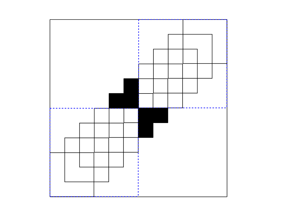
Figure 2: The support cubes of the wavelets and the bigger cubes ${\cal X}_{n,m}\times{\cal X}_{n,m}$.

Proof of Proposition 4.2.

Because $K_{k}$ is an orthogonal projection on a $(2k+1)$-dimensional space, Lemma 7.1 gives that the operator norm satisfies $\|K_{k}\|=1$ and that the numbers $k_{n}$ as in (4) but with ${\mu}_{2}=1$ are equal to $\int\int K_{k}^{2}\,d{\lambda}\,d{\lambda}=2k+1$.

By the change of variables $x_{1}-x_{2}=u$, $x_{1}+x_{2}=v$ we find, for any ${\varepsilon}\in(0,\pi]$, and $K_{k}(x_{1},x_{2})=D_{k}(x_{1}-x_{2})$,

$$\int_{-\pi}^{\pi}\!\!\int_{-\pi}^{\pi}1_{|x_{1}-x_{2}|>{\varepsilon}}K_{k}^{2}(x_{1},x_{2})\,dx_{1}\,dx_{2} =2\int_{\varepsilon}^{2\pi}\!\!\int_{u-2\pi}^{2\pi-u}D_{k}^{2}(u){\textstyle{\frac{1}{2}}}\,dv\,du$$

$$=2\int_{\varepsilon}^{2\pi}D_{k}^{2}(u)(2\pi-u)\,du.$$

By the symmetry of the Dirichlet kernel about $\pi$ we can rewrite $\int_{\pi}^{2\pi}D_{k}^{2}(u)(2\pi-u)\,du$ as $\int_{0}^{\pi}D_{k}^{2}(u)u\,du$. Splitting the integral on the right side of the preceding display over the intervals $({\varepsilon},\pi]$ and $(\pi,2\pi]$, and rewriting the second integral, we see that the preceding display is equal to

$$2\int_{\varepsilon}^{\pi}D_{k}^{2}(u)(2\pi-u)\,du+2\int_{0}^{\pi}D_{k}^{2}(u)u\,du=4\pi\int_{\varepsilon}^{\pi}D_{k}^{2}(u)\,du+2\int_{0}^{\varepsilon}D_{k}^{2}(u)u\,du.$$

For ${\varepsilon}=0$ this expression is equal to the square $L_{2}$-norm of the kernel $K_{k}$, which shows that $4\pi\int_{0}^{\pi}D_{k}^{2}(u)\,du=2k+1$. On the interval $({\varepsilon},\pi)$ the kernel $D_{k}$ is bounded above by $\bigl{(}2\pi\sin({\textstyle{\frac{1}{2}}}{\varepsilon})\bigr{)}^{-1}$. Therefore, the preceding display is bounded above by

$${4\pi\over\bigl{(}2\pi\sin({\textstyle{\frac{1}{2}}}{\varepsilon})\bigr{)}^{2}}\int_{\varepsilon}^{\pi}\,du+2{\varepsilon}\int_{0}^{\varepsilon}D_{k}^{2}(u)\,du\lesssim{1\over\sin^{2}({\textstyle{\frac{1}{2}}}{\varepsilon})}+{\varepsilon}k.$$

We conclude that, for small ${\varepsilon}>0$,

$${1\over 2k+1}\int_{-\pi}^{\pi}\!\!\int_{-\pi}^{\pi}1_{|x_{1}-x_{2}|>{\varepsilon}}K_{k}^{2}(x_{1},x_{2})\,dx_{1}\,dx_{2}\lesssim{\varepsilon}+{1\over{\varepsilon}^{2}k}.$$

This tends to zero as $k\rightarrow\infty$ whenever ${\varepsilon}={\varepsilon}_{k}\downarrow 0$ such that ${\varepsilon}\gg 1/\sqrt{k}$.

We choose a partition $(-\pi,\pi]=\cup_{m}{\cal X}_{n,m}$ in $M_{n}=2\pi/{\delta}$ intervals of length ${\delta}$ for ${\delta}\rightarrow 0$ with ${\delta}\gg{\varepsilon}$ and ${\varepsilon}$ satisfying the conditions of the preceding paragraph. Then the complement of $\cup_{m}{\cal X}_{n,m}\times{\cal X}_{n,m}$ is contained in $\{(x_{1},x_{2}):|x_{1}-x_{2}|>{\varepsilon}\}$ except for a set of $2(M_{n}-1)$ triangles, as indicated in Figure 3. In order to verify (6) it suffices to show that $(2k+1)^{-1}$ times the integral of $K_{k}^{2}$ over the union of the triangles is negligible. Each triangle has sides of length of the order ${\varepsilon}$, whence, for a typical triangle $\Delta$, by the change of variables $x_{1}-x_{2}=u$, $x_{2}=v$, and an interval $I$ of length of the order ${\varepsilon}$,

$$\mathop{\int\!\!\int}\limits_{\Delta}K_{k}^{2}(x_{1},x_{2})\,dx_{1}\,dx_{2}\lesssim\int_{I}\!\int_{0}^{\varepsilon}D_{k}^{2}(u)\,du\,dv\lesssim{\varepsilon}(2k+1).$$

Hence (6) is satisfied if $2(M_{n}-1){\varepsilon}\rightarrow 0$, i.e. ${\varepsilon}\ll{\delta}$.

Because $\int_{{\cal X}_{n,m}}\int_{X_{n,m}}K_{k}^{2}\,d({\lambda}\times{\lambda})$ is independent of $m$, (7) is satisfied as soon as the number of sets in the partitions tends to infinity.

Because $0\leq K_{k}\leq 2k+1$, condition (10) is implied by (11), which is satisfied if ${\delta}\ll n/k$.

The desired choices $1/\sqrt{k}\ll{\varepsilon}\ll{\delta}\ll n/k$ are compatible, as by assumption $k/n^{2}\rightarrow 0$.   

Figure 3: The triangles used in the proofs of Theorems 4.2 and 4.3, and the sets ${\cal X}_{n,m}\times{\cal X}_{n,m}$.

Proof of Proposition 4.3.

Without loss of generality we can assume that $\int|\phi|\,d{\lambda}=1$. By a change of variables

$$\int K_{\sigma}^{2}\,d(G\times G)={1\over{\sigma}}\int\phi^{2}(v)\int g(x-{\sigma}v)g(x)\,dx\,dv.$$

Here $\bigl{|}\int g(x-{\sigma}v)g(x)\,dx\bigr{|}\leq\|g\|_{\infty}$ and, as ${\sigma}\downarrow 0$,

$$\Bigl{|}\int g(x-{\sigma}v)g(x)\,dx-\int g^{2}(x)\,dx\Bigr{|}\leq\|g\|_{\infty}\int\bigl{|}g(x-{\sigma}v)-g(x)\bigr{|}\,dx\rightarrow 0,$$

for every fixed $v$, by the $L_{1}$-continuity theorem. We conclude by the dominated convergence theorem that ${\sigma}\int K_{\sigma}^{2}\,d(G\times G)\rightarrow\int g^{2}\,d{\lambda}\int\phi^{2}\,d{\lambda}$. Because ${\mu}_{2}$ is bounded away from 0 and $\infty$, the numbers $k_{n}$ defined in (4) are of the exact order ${\sigma}^{-1}$.

By another change of variables, followed by an application of the Cauchy-Schwarz inequality, for any $f\in L_{2}(G)$,

$$\int(K_{\sigma}f)^{2}\,dG =\int\Bigl{(}\int\phi(v)(fg)(x-{\sigma}v)\,dv\Bigr{)}^{2}\,dG(x)$$

$$\leq\|g\|_{\infty}^{2}\int\!\!\int|\phi|(v)(f^{2}g)(x-{\sigma}v)\,dv\,dx=\|g\|_{\infty}^{2}\int f^{2}g\,d{\lambda}.$$

Therefore, the operator norms of the operators $K_{\sigma}$ are uniformly bounded in ${\sigma}>0$.

We choose a partition $\mathbb{R}=\cup_{m}{\cal X}_{n,m}$ consisting of two infinite intervals $(-\infty,-a]$ and $(a,\infty)$ and a regular partition of the interval $(-a,a]$ in such a way that every partitioning set satisfies $G({\cal X}_{n,m})\leq{\delta}$. We can achieve this with a partition in $M_{n}=O(1/{\delta})$ sets.

Because $|K_{\sigma}|$ is bounded by a multiple of ${\sigma}^{-1}$, condition (10) is implied by (11), which takes the form ${\delta}/({\sigma}n)\rightarrow 0$, in view of Lemma 2.1.

For an arbitrary partitioning set ${\cal X}_{n,m}$,

$${\sigma}\int_{{\cal X}_{n,m}}\!\!\int_{{\cal X}_{n,m}}K_{\sigma}^{2}\,d(G\times G) \leq\int_{{\cal X}_{n,m}}\int\phi^{2}(v)\,g(x-{\sigma}v)g(x)\,dv\,dx$$

$$\leq\|g\|_{\infty}\int\phi^{2}(v)\,dv\,G({\cal X}_{n,m}).$$

It follows that (7) is satisfied as soon as ${\delta}\rightarrow 0$.

Finally, we verify condition (6) in two steps. First, for any ${\varepsilon}\downarrow 0$, by the change of variables $x_{1}-x_{2}=v$, $x_{2}=x$,

$${\sigma}\!\!\mathop{\int\!\!\int}\limits_{|x_{1}-x_{2}|>{\varepsilon}}K_{\sigma}^{2}\,d(G\times G) =\mathop{\int\!\!\int}\limits_{|v|>{\varepsilon}/{\sigma}}\phi^{2}(v)\,g(x-{\sigma}v)g(x)\,dx\,dv$$

$$\leq\|g\|_{\infty}\int_{|v|>{\varepsilon}/{\sigma}}\phi^{2}(v)\,dv.$$

This converges to zero as ${\sigma}\rightarrow 0$ for any ${\varepsilon}={\varepsilon}_{\sigma}>0$ with ${\varepsilon}\gg{\sigma}$. Second, for ${\varepsilon}\ll{\delta}$ the complement of the set $\cup_{m}{\cal X}_{n,m}\times{\cal X}_{n,m}$ is contained in $\{(x_{1},x_{2}):|x_{1}-x_{2}|>{\varepsilon}\}$ except for a set of $2(M_{n}-1)$ triangles, as indicated in Figure 3. In order to verify (6) it suffices to show that ${\sigma}$ times the integral of $K_{\sigma}^{2}$ over the union of the triangles is negligible. Each triangle has sides of length of the order ${\varepsilon}$, whence, for a typical triangle $\Delta$, with projection $I$ on the $x_{1}$-axis,

$${\sigma}\mathop{\int\!\!\int}\limits_{\Delta}K_{\sigma}^{2}\,d(G\times G)\lesssim\int_{I}\!\!\int_{|v|<{\varepsilon}/{\sigma}}\phi^{2}(v)\,g(x-{\sigma}v)g(x)\,dv\,dx\leq{\varepsilon}\|g\|_{\infty}\int\phi^{2}(v)\,dv.$$

The total contribution of all triangles is $2(M_{n}-1)$ times this expression. Hence (6) is satisfied if $2(M_{n}-1){\varepsilon}\rightarrow 0$, i.e. ${\varepsilon}\ll{\delta}$.

The preceding requirements can be summarized as ${\sigma}\ll{\varepsilon}\ll{\delta}\ll{\sigma}n$, and are compatible.   

Proof of Proposition 4.4.

Inequality (22) implies that $c_{j}(f)=0$ for every $f$ that vanishes outside the interval $(t_{j}^{\prime},t_{j+r}^{\prime})$, whence the representing function $g_{j}$ is supported on this interval. It follows that the function $(x_{1},x_{2})\mapsto N_{j}(x_{1})c_{j}(x_{2})$ vanishes outside the square $[t_{j}^{\prime},t_{j+r}^{\prime}]\times[t_{j}^{\prime},t_{j+r}^{\prime}]$, which has area of the order $l^{-2}$. We form a partition $(0,1]=\cup_{m}{\cal X}_{n,m}$ by selecting subsets $0=s_{0}^{l}<s_{1}^{l}<\cdots<s_{M_{n}}^{l}=1$ of the basic knot sequences such that $M_{n}^{-1}\lesssim s_{i+1}^{l}-s_{i}^{l}\lesssim M_{n}^{-1}$ for every $i$ and define ${\cal X}_{n,m}=(s_{m-1}^{l},s_{m}^{l}]$. The numbers $M_{n}$ are chosen integers much smaller than $l_{n}$, and we may set $s_{i}^{l}=t_{ip}^{l}$ for $p=\lfloor l_{n}/M_{n}\rfloor$.

Because $K_{k}$ is a projection on $S_{r}(T,d)$ and the function $x_{1}\mapsto K_{k}(x_{1},x_{2})$ is contained in $S_{r}(T,d)$ for every $x_{2}$, it follows that $\int K_{k}(x_{1},x_{2})K_{k}(x_{1},x_{2})\,dx_{1}=K_{k}(x_{2},x_{2})$ for every $x_{2}$, and hence

$$\int\!\!\int K_{k}(x_{1},x_{2})^{2}\,dx_{1}\,dx_{2}=\int K_{k}(x_{1},x_{1})\,d{\lambda}(x_{1})$$

$$\hskip 40.00006pt=\int\sum_{j}N_{j}(x_{1})c_{j}(x_{1})\,dx_{1}=\sum_{j}c_{j}(N_{j})=\sum_{j}1=k,$$

because the identities $N_{i}=K_{k}N_{i}=\sum_{j}c_{j}(N_{i})N_{j}$ imply that $c_{j}(N_{i})={\delta}_{ij}$ by the linear independence of the B-splines. Because the density of $G$ and the function ${\mu}_{2}$ are bounded above and below the $L_{2}(G\times G)$-norm $k_{n}$ as in (4) is of the same order as the dimension $k_{n}=r+l_{n}d$ of the spline space.

Inequality (22) implies that the norm of the linear map $c_{j}$, which is the infinity norm $\|c_{j}\|_{\infty}$ of the representing function, is bounded above by a constant times $(t_{j+r}^{\prime}-t_{j}^{\prime})^{-1}$, which is of the order $k_{n}$. Therefore,

$${1\over k_{n}}\int\!\!\int_{(\cup_{m}{\cal X}_{n,m}\times{\cal X}_{n,m})^{c}}K_{n}^{2}\ ({\mu}_{2}\times{\mu}_{2})\,d(G\times G)$$

$$\qquad\lesssim{1\over k_{n}}\,k_{n}^{2}\,\|{\mu}_{2}\|_{\infty}^{2}\,{\lambda}\Bigl{(}\bigcup_{j}(t_{j}^{\prime},t_{j+r}^{\prime}]\times(t_{j}^{\prime},t_{j+r}^{\prime}]-\bigcup_{m}(s_{m-1},s_{m}]\times(s_{m-1},s_{m}]\Bigr{)}.$$

The set in the right side is the union of $M_{n}$ cubes of areas not bigger than the area of the sets $(t_{j}^{\prime},t_{j+r}^{\prime}]\times(t_{j}^{\prime},t_{j+r}^{\prime}]$, which is bounded above by a constant times $k_{n}^{-2}$. (See Figure 2.) The preceding display is therefore bounded above by

$${1\over k_{n}}k_{n}^{2}\,\|{\mu}_{2}\|_{\infty}^{2}\,M_{n}\,{1\over k_{n}^{2}}.$$

For $M_{n}/k_{n}\rightarrow 0$ this tends to zero. This completes the verification of (6).

The verification of the other conditions follows the same lines as in the case of the wavelet basis.

References

-
[1]
J. Robins, L. Li, E. Tchetgen, A. van der Vaart,
Higher order influence
functions and minimax estimation of nonlinear functionals, in: Probability
and statistics: essays in honor of David A. Freedman, Vol. 2 of Inst.
Math. Stat. Collect., Inst. Math. Statist., Beachwood, OH, 2008, pp.
335–421.
doi:10.1214/193940307000000527.
URL http://dx.doi.org/10.1214/193940307000000527 - [2] P. J. Bickel, Y. Ritov, Estimating integrated squared density derivatives: sharp best order of convergence estimates, Sankhyā Ser. A 50 (3) (1988) 381–393.
- [3] L. Birgé, P. Massart, Estimation of integral functionals of a density, Ann. Statist. 23 (1) (1995) 11–29.
- [4] B. Laurent, Efficient estimation of integral functionals of a density, Ann. Statist. 24 (2) (1996) 659–681.
- [5] B. Laurent, Estimation of integral functionals of a density and its derivatives, Bernoulli 3 (2) (1997) 181–211.
- [6] B. Laurent, P. Massart, Adaptive estimation of a quadratic functional by model selection, Ann. Statist. 28 (5) (2000) 1302–1338.
-
[7]
J. Robins, L. Li, E. Tchetgen, A. W. van der Vaart,
Quadratic semiparametric
von Mises calculus, Metrika 69 (2-3) (2009) 227–247.
doi:10.1007/s00184-008-0214-3.
URL http://dx.doi.org/10.1007/s00184-008-0214-3 - [8] A. van der Vaart, Higher order tangent spaces and influence functions, Statist. Sci. 29 (4) (2014) 679–686. doi:10.1214/14-STS478.
- [9] E. Tchetgen, L. Li, J. Robins, A. van der Vaart, Higher order estimating equations for high-dimensional semiparametric models, preprint.
- [10] J. Robins, A. van der Vaart, Adaptive nonparametric confidence sets, Ann. Statist. 34 (1) (2006) 229–253.
-
[11]
N. C. Weber, Central limit
theorems for a class of symmetric statistics, Math. Proc. Cambridge Philos.
Soc. 94 (2) (1983) 307–313.
doi:10.1017/S0305004100061168.
URL http://dx.doi.org/10.1017/S0305004100061168 -
[12]
R. N. Bhattacharya, J. K. Ghosh,
A class of
-statistics and asymptotic normality of the number of -clusters,
J. Multivariate Anal. 43 (2) (1992) 300–330.
doi:10.1016/0047-259X(92)90038-H.
URL http://dx.doi.org/10.1016/0047-259X(92)90038-H - [13] S. R. Jammalamadaka, S. Janson, Limit theorems for a triangular scheme of -statistics with applications to inter-point distances, Ann. Probab. 14 (4) (1986) 1347–1358.
-
[14]
P. de Jong, A central limit theorem
for generalized quadratic forms, Probab. Theory Related Fields 75 (2) (1987)
261–277.
doi:10.1007/BF00354037.
URL http://dx.doi.org/10.1007/BF00354037 -
[15]
P. de Jong, A central
limit theorem for generalized multilinear forms, J. Multivariate Anal.
34 (2) (1990) 275–289.
doi:10.1016/0047-259X(90)90040-O.
URL http://dx.doi.org/10.1016/0047-259X(90)90040-O - [16] T. Mikosch, A weak invariance principle for weighted -statistics with varying kernels, J. Multivariate Anal. 47 (1) (1993) 82–102.
- [17] C. Morris, Central limit theorems for multinomial sums, Ann. Statist. 3 (1975) 165–188.
- [18] M. S. Ermakov, Asymptotic minimaxity of chi-squared tests, Teor. Veroyatnost. i Primenen. 42 (4) (1997) 668–695.
- [19] G. Kerkyacharian, D. Picard, Estimating nonquadratic functionals of a density using Haar wavelets, Ann. Statist. 24 (2) (1996) 485–507.
-
[20]
J. Robins, E. Tchetgen Tchetgen, L. Li, A. van der Vaart,
Semiparametric minimax rates,
Electron. J. Stat. 3 (2009) 1305–1321.
doi:10.1214/09-EJS479.
URL http://dx.doi.org/10.1214/09-EJS479 - [21] W. K. Newey, F. Hsieh, J. M. Robins, Twicing kernels and a small bias property of semiparametric estimators, Econometrica 72 (3) (2004) 947–962.
- [22] I. Daubechies, Ten lectures on wavelets, Vol. 61 of CBMS-NSF Regional Conference Series in Applied Mathematics, Society for Industrial and Applied Mathematics (SIAM), Philadelphia, PA, 1992.
- [23] R. A. DeVore, G. G. Lorentz, Constructive approximation, Vol. 303 of Grundlehren der Mathematischen Wissenschaften [Fundamental Principles of Mathematical Sciences], Springer-Verlag, Berlin, 1993.
- [24] A. W. van der Vaart, Asymptotic statistics, Vol. 3 of Cambridge Series in Statistical and Probabilistic Mathematics, Cambridge University Press, Cambridge, 1998.
- [25] E. Giné, R. Latala, J. Zinn, Exponential and moment inequalities for -statistics, in: High dimensional probability, II (Seattle, WA, 1999), Vol. 47 of Progr. Probab., Birkhäuser Boston, Boston, MA, 2000, pp. 13–38.