On an ordering-dependent generalization of Tutte polynomial

Abstract

A generalization of Tutte polynomial involved in the evaluation of the moments of the integrated geometric Brownian in the Ito formalism is discussed. The new combinatorial invariant depends on the order in which the sequence of contraction-deletions have been performed on the graph. Thus, this work provides a motivation for studying an order-dependent Tutte polynomial in the context of stochastic differential equations. We show that in the limit of the control parameters encoding the ordering going to zero, the multivariate Tutte-Fortuin-Kasteleyn polynomial is recovered.

1 Introduction

There is a deep connection between stochastic processes and quantum theory. As in quantum mechanics, an important role is played by the history of a process, in particular when the process is not ergodic. Moreover, if the noise of a certain stochastic process can be described by a Wiener process, then one can resort to many techniques developed for studying quantum field theories. This is true in particular for the case of the geometric Brownian motion. The geometric Brownian motion (GBM) is the stochastic process described by the stochastic differential equation:

$$df=\mu fdt+\sigma fdW_{t}\,,$$ (1)

where $W_{t}$ is a Wiener process and where $\mu,\sigma$ are constants, which parametrize the drift and the strength of the noise, respectively. The solution of equation (1) can be written, formally, as

$$f(W_{t},t)=\exp\left\{\left(\mu-\frac{\sigma^{2}}{2}\right)t+\sigma W_{t}\right\}.$$ (2)

The Geometric Brownian motion is used for modelling many phenomena in a variety of contexts [1, 2, 3, 4, 5]. This remains true for the case of the study of financial assets, where the distribution of returns can be approximated very often by a log-normal distribution [2, 1], at least in specific regimes. Yor provided various insights into the moments of the GBM, using as a starting point Girsanov theorem [6], and in particular in the case of the moments of its integral.

Recently, the properties of the moments of (2) were studied by means of combinatorics in [7], obtaining a closed formula, although cumbersome, for generic moments of the functional. Moreover, these functionals were shown to be involved in evaluating the averages of the solution of a logistic, stochastic differential equations. These logistic differential equations appear in the problem of the optimal leverage when one considers the microstructure properties of financial markets [8].

From the analysis provided in [7], the central quantities of interest emerged to be the functions $s_{k}$, defined by $\langle f(W_{t},t)^{n}\rangle=t^{n}\Gamma(n)s_{n}(\lambda_{1},\cdots,\lambda_{n})$, with $\lambda_{i}\equiv t(\mu+(k-i)\sigma^{2})$. One of the main results of [7], lays in the following proposition (Lemma 2 in [7]):

Proposition. Under the condition of Ito’s Wiener process, one has the following property for $s_{k}$:

$$s_{k}(\lambda_{1},\cdots,\lambda_{k})=\frac{e^{\lambda_{k}}}{\lambda_{k}}s_{k-1}(\lambda_{1},\cdots,\lambda_{k-1})-\frac{1}{\lambda_{k}}s_{k-1}(\lambda_{1},\cdots,\lambda_{k-2},\lambda_{k-1}+\lambda_{k})\,.$$ (3)

with $s_{0}=1$.

The recurrence relation (3) for the function $s_{k}$ can be solved to obtain a closed solution for the moments, and show that these functions can be written as a determinant of a linear operator [7]. One interesting observation is that (3) is very suggestive of a deletion-contraction rule performed on an abstract graph [9]. We are in the presence of a combinatorial object which can be described as a recursion relation of the form:

$$Z_{k}=\beta_{k}Z_{k-1}+\alpha_{k}Z_{k-1}^{\prime}\,,$$ (4)

where $Z_{k}$ and $Z_{k}^{\prime}$ are functions, $k$ is related to the number of edges of some graph $G$, $\alpha_{k}$ and $\beta_{k}$ coefficients associated with an edge of the graph being either contracted or deleted. In the present paper, we are interested in the mathematical properties of the relation (3) and explore in which sense one can actually consider this as the result of an underlying generalized Tutte polynomial [9]. This task presents several difficulties. As a first comment, we note that in order to describe the recurrence (3), one needs to formulate a combinatorial object similar to the multi-variate version of the Tutte polynomial [10], and rather in the form of the Fortuin and Kasteleyn (FK) [11]. Introduced in the study of random cluster models, the Tutte-FK polynomial on a graph $G(V,E)$, with edge weights $(p_{e})_{e\in E}$, satisfies in fact a recurrence relation as

$$Z(G,(p_{e}))=q_{e}\,Z(G-e,(p_{e^{\prime}\neq e}))+p_{e}\,Z(G/e,(p_{e^{\prime}\neq e}))\,,$$ (5)

where $p_{e}\in[0,1]$, $q_{e}$ is a “dual” weight chosen as $1-p_{e}$. In full generality, $p_{e}$ and $q_{e}$ can be elements of a commutative ring. We note that in (5), upon contraction and deletion, $Z(G/e)$ and $Z(G-e)$ keep the form of $Z(G)$ and become independent of the weights $p_{e}$ and $q_{e}$ of the edge $e$. This property is fundamental to ensure that the polynomial $Z(G)$ (as for any object falling in the universality class described by the Tutte polynomial) is independent of the order in which one performs the sequence of contraction and deletion of the edges of $G$. From the right hand side of (3), we note that the second function $s_{k-1}(\dots,\lambda_{k-1}+\lambda_{k})$ still keeps its dependence of the variable $\lambda_{k}$. This suggests that the combinatorial object that we seek is different from the usual Tutte-FK polynomial. If we want to extend the Tutte polynomial, it is therefore necessary to explicitly encode such a type of memory principle in the polynomial. As we will show, the memory encoded in the recursion relation in fact can be parametrized by the introduction of an ordering of the edges $(e_{\sigma(1)},e_{\sigma(2)},\dots,e_{\sigma(n)})$, where $n=|E|$ and $\sigma$ belongs to the symmetric group of $n$ elements.

Finally, we emphasize the fact that this work reports an extension of Tutte polynomial which depends on the order of the contraction-deletion. Such a type of polynomial have not been the main focus of the attention of combinatoricists, to the best of our knowledge. In [12], Bollobás and Riordan mention a possible extension of Tutte polynomial using noncommutative ring elements which is contraction-deletion-ordering-dependent and perhaps worth to investigate in the future. In a different but still close perspective, this work precisely provides an instance in which this ordering for the Tutte polynomial might be relevant in evaluating averages in exponentiated Wiener processes. We provide the generalized Tutte polynomial in Section 2, followed by conclusions in Section 3. Appendix A provides the proof of a technical lemma and, to illustrate the new graph invariant, we evaluate the generalized Tutte polynomial on a specific graph in Appendix B.

2 The recurrence relation of the generalized Tutte

The recurrence relation defined in (3) introduced in [7] can be thought as a modified contraction-deletion of the chain graph (see Fig.1). Our initial task is to generalize this recurrence relation to an arbitrary graph. Let us adopt the following considerations which clearly encompass the problem (3): let $R$ be a commutative ring and $T$ be a $R$-valued function defined on a graph $G(V,E)$. Let us assume that $T$ is defined on the set of edges weights $\{\lambda_{e}\}_{e\in E}$, $\lambda_{e}\in R$, and satisfies, for any edge $e$,

$$T(G;\{\lambda_{e}\})=\alpha(\lambda_{e})\,T(G/e;\{\tilde{\lambda}_{\tilde{e}\neq e}\})+\beta(\lambda_{e})\,T(G-e;\{\lambda^{\prime}_{e^{\prime}\neq e}\})\,,$$ (6)

where $\tilde{\lambda}_{\tilde{e}\neq e}=\tilde{\lambda}_{\tilde{e}\neq e}(\{\lambda_{e}\})$ and $\lambda^{\prime}_{e^{\prime}\neq e}=\lambda^{\prime}_{e^{\prime}\neq e}(\{\lambda_{e}\})$ are new edge weights of $G/e$ and $G-e$, respectively, and are functions of the former edge weights of $G$; $\alpha$ and $\beta$ are $R$-valued functions.

Figure 1: The chain graph $G$, $G-e_{n}$ and $G/e_{n}$, and their weights.

Performing successively the recurrence relation on a graph $G$, one ends with the boundary conditions (b.c.) $T(E_{m};\emptyset)=q_{m}\in R$, where $E_{m}$ is the graph made with only $m$ vertices and no edges. We refer to these b.c. as terminal forms of the contraction-deletion. $T$ is therefore a sum of contributions of the rough form $\approx(\prod\alpha(\cdot))(\prod\beta(\cdot))T(E_{m};\emptyset)$. At the end of the sequence of contraction-deletion operations, each terminal form can be uniquely mapped to a spanning subgraph of $G$. The existence of that bijection is guaranteed by the fact that the number of spanning subgraphs of $G$ is $2^{E}$, and this is precisely the number terminal forms. If we start from an edge-labelled graph $G$, the bijection becomes more apparent: starting from $G$ and following the unique path from the root to a given leaf $E_{m}$, we get a sequence of contracted and deleted edges of $G$. The unique spanning subgraph associated with the terminal form $E_{m}$ is the spanning subgraph of $G$ the edge set of which is the set of edges which have been contracted along the path to get $E_{m}$. Given the discussion above, the following statement is therefore straightforward:

Lemma 2.1.

The function $T(G;\{\lambda_{e}\})$ is a polynomial in the $\alpha$’s and $\beta$’s which admits a spanning subgraph expansion.

The function $T(G;-)$ factorizes along disconnected graphs, i.e. $T(G_{1}\cup G_{2};-)=T(G_{1};-)T(G_{2};-)$, if each contribution of spanning subgraph $A=A_{1}\cup A_{2}$ of $G=G_{1}\cup G_{2}$ will factorize between spanning subgraphs $A_{1}\subset G_{1}$ and $A_{2}\subset G_{2}$. Another important operation on abstract graphs is called the vertex-union or one-point-join operation on graphs. Under this operation, the ordinary Tutte factorizes $T(G_{1}\cdot G_{2})=T(G_{1})T(G_{2})$. In this work, we will check if these properties are satisfied by the new graph polynomial we introduce.

We must be more specific about the type of functions $\tilde{\lambda}_{\tilde{e}}$ and $\lambda^{\prime}_{e^{\prime}}$ that we will be interested in. Let us consider $R$ unital, a graph $G$ and its line graph $\mathcal{L}(G)$ [9]; consider moreover the adjacency matrix of $\mathcal{L}(G)$ that, by a slight abuse of notation, we write $A^{G}$. Given $G$ and an edge $e$ of $G$, we introduce the functions:

$\tilde{\lambda}:E(G/e)\to R$,   $\tilde{\lambda}(\tilde{e})=\lambda_{\tilde{e}}+\epsilon\,A^{G}_{\tilde{e}e}\lambda_{e}$ ;  $\epsilon\in R$ ;

$\lambda^{\prime}:E(G-e)\to R$,   $\lambda^{\prime}(e^{\prime})=\lambda_{e^{\prime}}+\epsilon^{\prime}\,A^{G}_{e^{\prime}e}\lambda_{e}$ ; $\epsilon^{\prime}\in R$ .

The functions $\tilde{\lambda}$ and $\lambda^{\prime}$ depend on a graph $G$ and one of its edges $e$; these might introduce shifts on the weights of all remaining edges (of $G/e$ and of $G-e$) sharing vertices with $e$. As an example of the variable shift mentioned above, in Fig.2 we show an example of deletion involving the line graph $A^{G}$: after each deletion (or contraction), the deleted variable modifies the edge variables of the resulting graph.

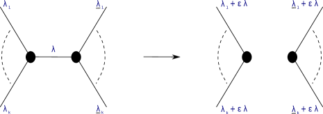
Figure 2: An example of deletion and “attaching” the deleted edge variable to the nearby edge variables. A similar rule applies also to the contraction, with the replacement of $\epsilon^{\prime}$ instead of $\epsilon$.

We are now in the position of introducing the problem treated in this work. Let $G$ be a graph with edge set $E$, $\epsilon,\epsilon^{\prime}\in R$. We are seeking for a function solution of the recurrence rule:

$$\forall e\in E,\quad T^{\epsilon,\epsilon^{\prime}}(G;\{\lambda_{e}\}_{e\in G}) = \alpha(\lambda_{e})\,T^{\epsilon,\epsilon^{\prime}}(G/e;\{\lambda_{\tilde{e}}+\epsilon\,A^{G}_{\tilde{e}e}\lambda_{e}\}_{\tilde{e}\in E(G/e)})$$ (7)

$$+ \beta(\lambda_{e})\,T^{\epsilon,\epsilon^{\prime}}(G-e;\{\lambda_{e^{\prime}}+\epsilon^{\prime}\,A^{G}_{e^{\prime}e}\lambda_{e}\}_{e^{\prime}\in E(G-e)})\,;$$ (9)

$$T^{\epsilon,\epsilon^{\prime}}(E_{m};\emptyset) = q_{m}\,.$$ (11)

For $\epsilon=\epsilon^{\prime}=0$, this combinatorial object reduces to Tutte polynomial. However, as we will see, the general case requires extra care.

2.1 Solving the ordering-dependent Tutte polynomial

The general recurrence rule (7) is radically different from an ordinary contraction-deletion rule because of the ordering-dependent evaluation of the recurrence to specify $T^{\epsilon,\epsilon^{\prime}}$. Note that, as stated above, since the recurrence rule holds for any initial edge $e$, it is not clear whether or not (7) has a general solution for arbitrary parameters $\epsilon$ and $\epsilon^{\prime}$. However, if we specify an ordering in the edges, which is determined by a permutation $\sigma\in\mathfrak{S}(n)$, $(e_{\sigma(1)},\dots,e_{\sigma(n)})$ and if we perform a contraction and deletion of each edge in the order $e_{\sigma(1)}\to e_{\sigma(2)}\to\dots\to e_{\sigma(n)}$, then we claim that the problem (7) has a solution if $T^{\epsilon,\epsilon^{\prime}}$ depends on the ordering $\sigma$. To write an explicit expression of this solution, we first introduce compact notations. Note that, since the general case can be easily recovered from the following results, we will focus on the simple case when $\sigma=id$, namely, when the edges are contracted and deleted according to the sequence $1\to 2\to 3\to\dots\to n$.

We introduce, for a given edge $e_{j}$,

$$G\cdot_{j}=\left\{\begin{array}[]{l}G/e_{j}\,,\;\;\text{if $e_{j}$ is contracted }\\ G-e_{j}\,,\;\;\text{if $e_{j}$ is deleted }\end{array}\right.$$ (14)

so that, for successive operations, the notation $G\cdot_{1}\cdot_{2}\cdots\cdot_{k}$, $k\leq n,$ provides a unique identification of the series of contractions or deletions. Then, given $(m,n)\notin\{1,\dots,k\}^{\times 2}$, we introduce

$$A^{(k)}_{mn}=A^{G\cdot_{1}\cdot_{2}\cdots\cdot_{k}}_{e_{m},e_{n}}$$ (15)

the matrix element of the adjacency matrix of $\mathcal{L}(G\cdot_{1}\cdot_{2}\cdots\cdot_{k})$ associated with vertices dual of $e_{m}$ and $e_{n}$. By convention, we set $A^{(0)}=A^{G}$. In the same vein, simplifying the labelling of $\lambda_{e_{j}}$, we shall use $\lambda_{j}$.

Consider an edge $e_{j}$ and a spanning subgraph $B$ of $G$, then define the following function on $R$

$$\gamma_{B}(x_{j})=\left\{\begin{array}[]{l}\alpha(x_{j})\,,\;\;\text{if $e_{j}\in B$ }\\ \beta(x_{j})\,,\;\;\text{if $e_{j}\notin B$}\end{array}\right.$$ (18)

for $x_{j}=x(e_{j})\in R$, and

$$\epsilon_{B}^{j}=\left\{\begin{array}[]{l}\epsilon\,,\;\;\text{if $e_{j}\in B$ }\\ \epsilon^{\prime}\,,\;\;\text{if $e_{j}\notin B$}\end{array}\right.$$ (21)

The following statement holds:

Theorem 2.1.

Let $G$ be a graph with edge set $E$, $|E|=n$. Consider a labelling of edges of $G$ such that $\{e_{j}\}_{j=1,\dots,n}$, and a family of edge weights $\{\lambda_{e_{j}}=\lambda_{j}\}_{j=1,\dots,n}$. Let $q$, $\epsilon$ and $\epsilon^{\prime}$ be elements in a commutative and unital ring $R$. A function $P^{\epsilon,\epsilon^{\prime}}(G;q;\{\lambda_{j}\})\in R$, solving the recurrence relation

$$P^{\epsilon,\epsilon^{\prime}}(G;q;\{\lambda_{j}\})=$$ (22)

$$\alpha(\lambda_{1})\,P^{\epsilon,\epsilon^{\prime}}(G/e_{1};\,q;\,\{\lambda_{j}+\epsilon A^{(0)}_{j1}\lambda_{1}\}_{j\neq 1})+\beta(\lambda_{1})\,P^{\epsilon,\epsilon^{\prime}}(G-e_{1};\,q;\,\{\lambda_{j}+\epsilon^{\prime}A^{(0)}_{j1}\lambda_{1}\}_{j\neq 1})\,;$$ (23)

(24)

$$P^{\epsilon,\epsilon^{\prime}}(E_{m};\,q;\emptyset)=q^{m}\,,$$ (25)

is of the form

$$P^{\epsilon,\epsilon^{\prime}}(G;q;\{\lambda_{j}\})=\sum_{B\subset G}q^{k(B)}\;\prod_{j=1}^{n}\gamma_{B}(\widehat{\lambda}_{j;B}\big{(}\{\lambda_{l}\}_{l\leq j})\big{)}\,,$$ (26)

where the sum is performed over the set of spanning subgraphs $B$ of $G$, $k(B)$ is the number of connected components of $B$, and, $\forall B$, one has

$$\forall k\geq 1\,, \widehat{\lambda}_{k;B}(\{\lambda_{l}\}_{l\leq k}))=\sum_{\ell=1}^{k}C_{k\ell;B}(G;\epsilon,\epsilon^{\prime})\lambda_{\ell}\,,$$ (27)

$$\text{ for }\,k=\ell\geq 1\,, C_{kk;B}(G;\epsilon,\epsilon^{\prime})=1\,,$$ (29)

$$\text{ for }\,k=\ell+1\,, C_{k(k-1);B}(G;\epsilon,\epsilon^{\prime})=\mathcal{A}_{k(k-1);B}(Q_{0})\,,$$ (31)

$$\forall k>\ell+1\geq 1\,, C_{k\ell;B}(G;\epsilon,\epsilon^{\prime})=\sum_{p=0}^{k-\ell-1}\sum_{\stackrel{{\scriptstyle Q_{p}\subseteq\{\ell+1,\dots,k-1\}}}{{|Q_{p}|=p}}}\mathcal{A}_{k\ell;B}(Q_{p})\,,$$ (33)

where

$$\text{for }\,Q_{0}=\emptyset,\;\;\mathcal{A}_{k\ell;B}(Q_{0})=\epsilon_{B}^{\ell}A^{(\ell-1)}_{k\ell}\,,$$ (34)

(35)

$$\text{for }\,Q_{p\geq 1}=\{j^{Q}_{1},\dots,j^{Q}_{p}\}\neq\emptyset,\;\;\ell+1\leq j^{Q}_{1}<j_{2}^{Q}<\dots<j^{Q}_{p}\leq k-1\,,$$ (36)

(37)

$$\mathcal{A}_{k\ell;B}(Q_{p})=\Big{(}\epsilon^{\ell}_{B}\prod_{a=1}^{p}\epsilon^{j^{Q}_{a}}_{B}\Big{)}\Big{[}A^{(j^{Q}_{p}-1)}_{kj^{Q}_{p}}\Big{(}\prod_{i=2}^{p}A^{(j^{Q}_{i-1}-1)}_{j^{Q}_{i}j^{Q}_{i-1}}\Big{)}A^{(\ell-1)}_{j^{Q}_{1}\ell}\Big{]}\;.$$ (38)

To prove this proposition, we rely on the following

Lemma 2.2.

For all $k>1$, and all $B$, $B\subset G$,

$$C_{k1;B}(G;\epsilon,\epsilon^{\prime})=\epsilon^{1}_{B}\sum_{\ell>1}^{k}A^{(0)}_{\ell 1}C_{k\ell;B}(G;\epsilon,\epsilon^{\prime})\,.$$ (39)

Proof.

See Appendix A. ∎

Proof of Theorem 2.1.

We note that the relation (25) is a direct consequence of (26). We concentrate on the recurrence by applying the contraction and deletion to $e_{1}$. We proceed like in the proof of the regular Tutte polynomial case: consider all terms in (26) associated with subgraphs of $G$ having $e_{1}$ and all terms associated with those which do not. We must prove that

$$\sum_{B\subset G;\,e_{1}\in B}q^{k(B)}\;\prod_{j=1}^{n}\gamma_{B}(\widehat{\lambda}_{j;B}(\{\lambda_{l}\})) = \alpha(\lambda_{1})\,P^{\epsilon,\epsilon^{\prime}}(G/e_{1};q;\,\{\lambda_{j}+\epsilon A^{(0)}_{j1}\lambda_{1}\}_{j>1})$$ (40)

$$= \alpha(\lambda_{1})\sum_{B\subset G/e_{1}}q^{k(B)}\;\prod_{j=2}^{n}\gamma_{B}(\widehat{\lambda}_{j;B}(\{\lambda_{l}+\epsilon A^{(0)}_{l1}\lambda_{1}\}))\,,$$ (42)

$$\sum_{B\subset G;\,e_{1}\notin B}q^{k(B)}\;\prod_{j=1}^{n}\gamma_{B}(\widehat{\lambda}_{j;B}(\{\lambda_{l}\})) = \beta(\lambda_{1})\,P^{\epsilon,\epsilon^{\prime}}(G-e_{1};q;\,\{\lambda_{j}+\epsilon^{\prime}A^{(0)}_{j1}\lambda_{1}\}_{j>1})$$ (44)

$$= \beta(\lambda_{1})\sum_{B\subset G-e_{1}}q^{k(B)}\;\prod_{j=2}^{n}\gamma_{B}(\widehat{\lambda}_{j;B}(\{\lambda_{l}+\epsilon^{\prime}A^{(0)}_{l1}\lambda_{1}\}))\,.$$ (46)

Since the variable $q$ which describe the number of connected components present no particular difficulty, we focus on the products. We will prove the above statement in the following way: to each subgraph $B\subset G$, and for each factor in the product $\prod_{j=1}^{n}\gamma_{B}(\widehat{\lambda}_{j}(-))$, we assign a unique and equal factor in the product $\gamma_{B}(\lambda_{1})\prod_{j=2}^{n}\gamma_{B^{\prime}}(\widehat{\lambda}_{j}(-))$, labelled by a subgraph $B^{\prime}\in G\cdot_{1}$.

Let us now consider the expansion, for a given subgraph $B$,

$$\prod_{j=1}^{n}\gamma_{B}(\widehat{\lambda}_{j;B}(\{\lambda_{l}\}))=\gamma_{B}\Big{(}C_{11;B}(G;\epsilon,\epsilon^{\prime})\lambda_{1}\Big{)}\prod_{j=2}^{n}\gamma_{B}(\widehat{\lambda}_{j;B}(\{\lambda_{l}\}))$$ (49)

(50)

$$=\gamma_{B}(\lambda_{1})\prod_{j=2}^{n}\gamma_{B}\Big{(}C_{j1;B}(G;\epsilon,\epsilon^{\prime})\lambda_{1}+\sum_{\ell>1}^{k}C_{j\ell;B}(G;\epsilon,\epsilon^{\prime})\lambda_{\ell}\Big{)}\,.$$ (51)

Using Lemma 2.2, we expand $C_{j1;B}$ in terms of $C_{j\ell}$ and write

$$\prod_{j=1}^{n}\gamma_{B}(\widehat{\lambda}_{j;B}(\{\lambda_{l}\})) = \gamma_{B}(\lambda_{1})\prod_{j=2}^{n}\gamma_{B}\Big{(}\epsilon^{1}_{B}\sum_{\ell>1}^{j}A^{(0)}_{\ell 1}C_{j\ell;B}(G;\epsilon,\epsilon^{\prime})\lambda_{1}+\sum_{\ell>1}^{k}C_{j\ell;B}(G;\epsilon,\epsilon^{\prime})\lambda_{\ell}\Big{)}$$ (52)

$$= \gamma_{B}(\lambda_{1})\prod_{j=2}^{n}\gamma_{B}\Big{(}\sum_{\ell>1}^{j}C_{j\ell;B}(G;\epsilon,\epsilon^{\prime})\left(\lambda_{\ell}+\epsilon^{1}_{B}A^{(0)}_{\ell 1}\lambda_{1}\right)\Big{)}$$ (54)

$$= \gamma_{B}(\lambda_{1})\prod_{j=2}^{n}\gamma_{B}\Big{(}\widehat{\lambda}_{j}\big{(}\{\lambda_{\ell}+\epsilon^{1}_{B}A^{(0)}_{\ell 1}\lambda_{1}\}_{1<\ell\leq j}\big{)}\Big{)}\,.$$ (56)

Now, depending on whether $e_{1}$ belongs to $B$ or not, we can provide more informations on the initial factor $\gamma_{B}(\lambda_{1})$ in (40). If $e_{1}\notin B$, then $B\subset G$ is uniquely mapped to $B\in G-e_{1}$, with the same $\gamma_{B}(\widehat{\lambda}_{j>1})$; if $e_{1}\in B$, then $B\subset G$ is uniquely mapped to $B/e_{1}$, mapping $\gamma_{B}(\widehat{\lambda}_{j>1}\big{)}$ to $\gamma_{B/e_{1}}(\widehat{\lambda}_{j>1})$. Thus (40) holds. ∎

To obtain the $\sigma$-ordering-dependent polynomial $P^{\epsilon,\epsilon^{\prime}}(G;\sigma;q;\{\lambda_{j}\})$, the sums and products involved in the definition of $\widehat{\lambda}_{j}$ and $C_{k\ell}$ in (27) and (38) must be handled a little bit differently. Indeed, as they stand in these equations, they depend explicitly on the ordering $\sigma=id$. Reformulated in a full-fledged form using the ordering $\sigma(1)\to\dots\to\sigma(k)$, we can turn these symbols into $\widehat{\lambda}_{\sigma(j)}$ and $C_{\sigma(k)\sigma(\ell)}$. However, this turns out to be cumbersome in notations and does not add much to the discussion. So we will refrain to give their general formulae in their most expanded form.

To make clear how the generalized Tutte polynomial is evaluated, we have provided a worked out example in App. B.

2.2 Reductions

We do have the following limiting cases:

- the reduction to the Tutte-FK polynomial is direct by setting

$$Z(G;q;(\lambda_{e}))=P^{\epsilon=0,\epsilon^{\prime}=0}(G;q;\{\lambda_{e}\})\quad\text{with}\quad\alpha(\lambda_{e})=\lambda_{e}\,,\quad\beta(\lambda_{e})=1-\lambda_{e}\,,$$ (57)

with appropriate constraints $q_{m}=q^{m}$, $q\in R$, which represents an ordering-independent system.

- The recurrence (3) obeyed by function $s_{k}$ can be recovered by setting $G=C_{n}$ the chain graph with $n$ edges,

$$s_{n}(\{\lambda_{e}\})=T^{\epsilon=1,\epsilon^{\prime}=0}(C_{n};q=1;\{\lambda_{e}\})\quad\text{with}\quad\alpha(\lambda_{e})=\frac{e^{\lambda_{e}}}{\lambda_{e}}\,,\quad\beta(\lambda_{e})=-\frac{1}{\lambda_{e}}\,,$$ (58)

where we have made the choice that the deletion procedure will be associated with the ordering-dependency of the system.

- Setting all weights to a constant, i.e. $\lambda_{j}=\lambda$, and the ordering parameters $\epsilon$ and $\epsilon^{\prime}$ to 1, one should get a 3-parameter deformation of the standard Tutte polynomial (the parameters will be $(q,\alpha(\lambda),\beta(\lambda))$). The deformed invariant can be explicitly identified from the above formulae and its properties will be investigated elsewhere.

2.3 Properties of the generalized Tutte

We investigate now if the polynomial $P^{\epsilon,\epsilon^{\prime}}$ factorizes along connected components. Consider the graph $G=G_{1}\cup G_{2}$ made of disconnected graphs $G_{1}$ and $G_{2}$, with sets $E_{1}$ and $E_{2}$ of edges, respectively. Let us denote $|E_{1}|=n_{1}$ and $|E_{2}|=n_{2}$. Given an ordering $\sigma$ of the edges of $G$, we want to infer two orderings $\sigma_{1}\in\mathfrak{S}_{n_{1}}$ and $\sigma_{2}\in\mathfrak{S}_{n_{1}}$ of the edges in the two separate graphs $G_{1}$ and $G_{2}$, respectively. A simple listing achieves this: construct the image of $\sigma_{1}$ by listing all edges of $G_{1}$ in their order of appearance in $\sigma$, and then choose the image of $\sigma_{2}$ to be the rest of the edges (of $G_{2}$) keeping again their order of appearance in $\sigma$. The two permutations $\sigma_{1}$ and $\sigma_{2}$ will be called induced orderings (on $E_{1}$ and $E_{2}$) from $\sigma$.

Then, we have

$$P^{\epsilon,\epsilon^{\prime}}(G;\sigma=id;q;\{\lambda_{j}\})=\sum_{B_{1}\cup B_{2}\subset G_{1}\cup G_{2}}q^{k(B_{1})}q^{k(B_{2})}\prod_{j=1}^{n_{1}+n_{2}}\gamma_{B_{1}\cup B_{2}}(\widehat{\lambda}_{j}(\{\lambda_{l}\}))\;;$$ (59)

(60)

$$\prod_{j=1}^{n_{1}+n_{2}}\gamma_{B_{1}\cup B_{2}}(\widehat{\lambda}_{j}(\{\lambda_{\sigma(l)}\}))=\Big{[}\prod_{j=1}^{n_{1}}\gamma_{B_{1}\cup B_{2}}(\widehat{\lambda}_{\sigma_{1}(j)}(\{\lambda_{l}\}))\Big{]}\Big{[}\prod_{j=1}^{n_{2}}\gamma_{B_{1}\cup B_{2}}(\widehat{\lambda}_{\sigma_{2}(j)}(\{\lambda_{l}\}))\Big{]}.$$ (61)

For a disconnected graph $G_{1}\cup G_{2}$, there is an ordering of the edges of $G_{1}\cup G_{2}$ such that the matrix $A^{(k)}$ of $G_{1}\cup G_{2}$ will always appear block diagonal (an edge of $G_{1}$ cannot have a common vertex with any edge of $G_{2}$ after an arbitrary number of contractions and deletions). This implies that the contraction or deletion of an edge in a graph, say $G_{1}$, does not affect the variables in the other graph $G_{2}$ (and vice versa). For any $k\leq n_{1}+n_{2}$, there exists $k_{1}$ and $k_{2}$, such that $k=k_{1}+k_{2}$ and

$$(G_{1}\cup G_{2})\cdot_{1}\cdot_{2}\dots\cdot_{k}=(G_{1}\cdot_{\sigma_{1}(1)}\cdot_{\sigma_{1}(2)}\dots\cdot_{\sigma_{1}(k_{1})})\cup(G_{2}\cdot_{\sigma_{2}(1)}\cdot_{\sigma_{2}(2)}\dots\cdot_{\sigma_{2}(k_{2})})\,.$$ (62)

We stress now two important points: (1) the definitions of $\widehat{\lambda}_{\sigma_{1}(j)}$ and $\widehat{\lambda}_{\sigma_{2}(j)}$ can be now restricted to the adjacency matrix of the line graphs of $G_{1}$ and $G_{2}$, respectively, and (2), given $i\in\{1,2\}$, the function $\gamma_{B_{1}\cup B_{2}}(\widehat{\lambda}_{\sigma_{i}(j_{i})})$, $j_{i}=1,\dots,n_{i}$, becomes independent of $B_{i^{\prime}\neq i}$ and it is exactly the same as $\gamma_{B_{i}}(\widehat{\lambda}_{\sigma_{i}(j_{i})})$, $j_{i}=1,\dots,n_{i}$, $i=1,2$. Therefore, the following proposition holds:

Proposition 2.1 (Factorization under disjoint union).

Let $G_{1}$ and $G_{2}$ two graphs. Consider an ordering of the edges of $G_{1}\cup G_{2}$, then there exist two induced orderings of the edges, $\sigma_{1}$ of $G_{1}$ and $\sigma_{2}$ of $G_{2}$, and

$$P^{\epsilon,\epsilon^{\prime}}(G_{1}\cup G_{2};\sigma=id;q;\{\lambda_{j}\}_{j=1}^{n_{1}+n_{2}})=P^{\epsilon,\epsilon^{\prime}}(G_{1};\sigma_{1};q;\{\lambda_{j}\}_{j=1}^{n_{1}})P^{\epsilon,\epsilon^{\prime}}(G_{2};\sigma_{2};q;\{\lambda_{j}\}_{j=1}^{n_{2}})\,.$$ (63)

Like the Tutte polynomial, the polynomial $P^{\epsilon,\epsilon^{\prime}}$ obeys the factorization property under disjoint union operation. It is also immediate that given two orderings in $G_{1}$ and $G_{2}$, one can trivially construct an ordering of edges of $G_{1}\cup G_{2}$ (by concatenating these) such that the above equality still holds. However, the factorization property under one-point-join operation will fail for $P^{\epsilon,\epsilon^{\prime}}$ because joining two graphs by a vertex affects the structure of the adjacency matrices. Simple counter-examples exist can be easily checked by the reader.

2.4 Towards a noncommutative Tutte polynomial

Bollobás and Riordan [12] mention the likely existence of a Tutte polynomial on a noncommutative ring. We comment here another possibility to identify a noncommutative Tutte polynomial using a noncommutative/nonassociative algebra of weight functions which is based on the generalized polynomial found in this work. For simplicity, and because we need an integration measure, we will restrict to $R=\mathbb{R}$, the field of real numbers. The discussion below is purely formal. However, it can certainly be made rigorous using the appropriate functional space.

The polynomial $P^{\epsilon,\epsilon^{\prime}}(G;-)$ involves several convolutions of functions $\alpha$ and $\beta$ that we symbolize by $\gamma_{B}$. Indeed, we can introduce a family of kernels $\{K_{B}\}_{B\subset G}$ such that

$$P^{\epsilon,\epsilon^{\prime}}(G;q;\{\lambda_{j}\}) = \sum_{B\subset G}q^{k(B)}\int_{\tilde{\lambda}_{j}\in\mathbb{R}}[\prod_{j}d\tilde{\lambda}_{j}]\;\;K_{B}(\{\lambda_{j}\};\{\tilde{\lambda}_{j}\})\gamma_{B}(\tilde{\lambda}_{1})\cdots\gamma_{B}(\tilde{\lambda}_{n})$$ (64)

$$= \sum_{B\subset G}q^{k(B)}\;(\gamma_{B}^{1},\gamma_{B}^{2},\dots,\gamma_{B}^{n})_{\star_{K_{B}}}(\{\lambda_{j}\}_{j\geq 1})\,,$$ (66)

where $\star_{K_{B}}$ is a $n$-ary law with kernel $K_{B}$ which convolutes $n$ functions $\gamma_{B}^{j}\in\{\alpha,\beta\}$, and which gives as an output a function. The kernel $K$ can be thought of as a tensor product of delta-distributions which enforces the value of the $j$th component $\gamma(\tilde{\lambda}_{j})$ to the corresponding value appearing in the general formula (26). In general, $n$-ary laws are nonassociative (bracketing matters) and noncommutative (ordering the functions matters). In the above specific instance, because the kernel $K_{B}$ can be factorized

$$K_{B}=\delta(\tilde{\lambda}_{1}-\lambda_{1})\delta(\tilde{\lambda}_{2}-\widehat{\lambda}_{2;B}(\lambda_{1},\lambda_{2}))\dots\delta(\tilde{\lambda}_{n}-\widehat{\lambda}_{n;B}(\{\lambda_{l}\}_{l\leq n}))\,,$$ (67)

the above $\star_{K_{B}}$-product factorizes in binary laws,

$$(((\gamma_{B}^{1}\star_{K_{B};1}\gamma_{B}^{2})\star_{K_{B};2}\gamma_{B}^{3})\dots)\star_{K_{B};n-1}\gamma_{B}^{n}\,,$$ (68)

where the $\star_{K_{B};j}$-product is associated with the kernel

$$\delta\big{(}\tilde{\lambda}_{1}-\lambda_{1})\delta(\tilde{\lambda}_{2}-\widehat{\lambda}_{2;B}(\lambda_{1},\lambda_{2}))\dots\delta(\tilde{\lambda}_{j+1}-\widehat{\lambda}_{j+1;B}(\{\lambda_{l}\}_{l\leq j+1})\big{)}\,.$$ (69)

In this sense, an ordering-dependent Tutte polynomial would be realized in terms of a noncommutative algebra of functions endowed with several binary laws and it will obey

$$P^{\epsilon,\epsilon^{\prime}}(G;q;\{\lambda_{j}\})=\Big{[}\alpha\star_{1}\,P^{\epsilon,\epsilon^{\prime}}(G/e_{1};\,q;\,\{\lambda_{j}\}_{j\neq 1})\Big{]}(\lambda_{1})+\Big{[}\beta\star^{\prime}_{1}\,P^{\epsilon,\epsilon^{\prime}}(G-e_{1};\,q;\,\{\lambda_{j}\}_{j\neq 1})\Big{]}(\lambda_{1})$$ (70)

(71)

$$=\alpha(\lambda_{1})\,P^{\epsilon,\epsilon^{\prime}}(G/e_{1};\,q;\,\{\lambda_{j}+\epsilon A^{(0)}_{j1}\lambda_{1}\}_{j\neq 1})+\beta(\lambda_{1})\,P^{\epsilon,\epsilon^{\prime}}(G-e_{1};\,q;\,\{\lambda_{j}+\epsilon^{\prime}A^{(0)}_{j1}\lambda_{1}\}_{j\neq 1})\,.$$ (72)

up to b.c.. Note that we have made a choice of the kernels of $\star_{1}$ and $\star^{\prime}_{1}$ in order to write the convolution $\alpha\star_{1}\,P^{\epsilon,\epsilon^{\prime}}(G/e_{1};-)$ and $\beta\star^{\prime}_{1}\,P^{\epsilon,\epsilon^{\prime}}(G-e_{1};-)$ in the appropriate form to match the result. We could have chosen a different kernel and impose that it is $P^{\epsilon,\epsilon^{\prime}}(G/e_{1};-)\star_{1}\alpha$ and $P^{\epsilon,\epsilon^{\prime}}(G-e_{1};-)\star_{1}\beta$ which give the correct answer. Thus we can choose to convolute the functions $\alpha$ and $\beta$ either on the left or on the right of the reduced polynomials and this exhibits the richness of this framework.

2.5 A realization with graph with half-edges

Graph with half-edges are useful in the context of Quantum Field Theory. Half-edges represent external fields or probes used to measure higher energetic processes. Recently this type of graphs have investigated in several contexts (QFT, matrix models ribbons graphs, tensor graphs) [13, 14, 15]. In particular, in [15], Avohou et al. discussed an extension of Tutte polynomial to this type of graphs which satisfies a recurrence relation called “contraction and cut” relation. The cut operation on an edge $e\in G$ (denoted $G\vee e$) is intuitive: one deletes the edge and let two half-edges at its end vertex or vertices. The Tutte polynomial on half-edged graphs satisfies a recurrence rule of the form, for any regular edge $e$, [15]:

$$T_{G}=T_{G\vee e}+T_{G/e}=t_{e}^{2}T_{G-e}+T_{G/e}\,,$$ (73)

where $t_{e}$ is a new variable associated with half-edges obtained from $e$ after the cut in the graph $G$. One can quickly realize that this is an evaluation of the usual Tutte polynomial by its universality theorem. What it is important now to mention is the following: the half-edges let attached to the graph after cutting edges might play precisely the role of a memory of the system. Indeed, whenever we cut an edge, the data of that edge is not totally removed from the graph and might be encoded using the presence of the half-edges. This track deserves to be further investigated.

3 Concluding remarks and perspectives

In this work, motivated by the recursion relation appearing in evaluating the moments of the integrated geometric Brownian motion, we have provided an extension of the Tutte-Fortuin-Kasteleyn polynomial depending on the contraction-deletion ordering. Such dependence emerges naturally from the recursion property proved in [7] for generic moments of the integrated geometric Brownian motion. Our work entails several interesting consequences. First, we have provided a possible generalization of Tutte polynomial which reduces to the Tutte-FK polynomial in a specific limit of the control parameters. Moreover, we have provided sufficient evidence motivating the study of Tutte polynomials which depend on the ordering of contractions. We have suggested that this generalization might be based on a noncommutative version of the Tutte polynomial, arising from the nonassociative properties of a star product emerging from the ordering of the contraction-deletions. As it is well known, the Tutte polynomial is associated to the partition function of the Potts model [10], and in the context of Quantum Field Theory [13], the Tutte-Symanzik polynomial in fact provides a parametric representation of Feynman amplitudes. Thus, quite intriguingly, our work might relate indirectly stochastic models in one dimensions [7, 8] with the perturbation theory of Quantum Field Theories. One of the main perspectives of the combinatorial approaches presented here is their extension for the study of the properties of other stochastic models which can be formally written as a perturbation expansion involving the integrated geometric Brownian motion.

Appendix A Proof of Lemma 2.2

Let us recall Lemma 2.2:

Lemma A.1.

In notations of Theorem 2.1, for all $k>1$,

$$C_{k1;B}(G;\epsilon,\epsilon^{\prime})=\epsilon^{1}_{B}\sum_{\ell>1}^{k}A^{(0)}_{\ell 1}C_{k\ell;B}(G;\epsilon,\epsilon^{\prime})\,.$$ (A.1)

Working at fixed graphs $B$ and $G$, we simplify the notations as follows: $C_{k\ell;B}(G;\epsilon,\epsilon^{\prime})=C_{k\ell}$. We prove the relation (A.1) by recurrence on $k$. At $k=2$, we have $C_{21}=\epsilon^{1}_{B}A^{(0)}_{21}=\epsilon^{1}_{B}A^{(0)}_{21}C_{22}$. Let us assume the result holds at $k$. Calculating the r.h.s of (A.1) at the next order $k+1$, we find

$$\epsilon^{1}_{B}\sum_{\ell>1}^{k+1}A^{(0)}_{\ell 1}C_{(k+1)\ell}=\epsilon^{1}_{B}A^{(0)}_{(k+1)1}+\epsilon^{1}_{B}A^{(0)}_{k1}C_{(k+1)k}+\epsilon^{1}_{B}A^{(0)}_{(k-1)1}C_{(k+1)(k-1)}$$ (A.2)

$$+\epsilon^{1}_{B}\sum_{\ell>1}^{k-2}A^{(0)}_{\ell 1}\sum_{p=0}^{(k+1)-\ell-1}\sum_{\stackrel{{\scriptstyle Q_{p}\subseteq\{\ell+1,\dots,(k+1)-1\}}}{{|Q_{p}|=p}}}\mathcal{A}_{(k+1)\ell;B}(Q_{p})$$ (A.3)

(A.4)

(A.5)

$$=\epsilon^{1}_{B}A^{(0)}_{(k+1)1}+\epsilon^{1}_{B}A^{(0)}_{k1}C_{(k+1)k}+\epsilon^{1}_{B}A^{(0)}_{(k-1)1}C_{(k+1)(k-1)}$$ (A.6)

$$+\epsilon^{1}_{B}\sum_{\ell>1}^{k-2}A^{(0)}_{\ell 1}\sum_{p=0}^{k-\ell}\Big{[}\sum_{\stackrel{{\scriptstyle Q_{p}\subseteq\{\ell+1,\dots,k\}}}{{|Q_{p}|=p\;\text{and}\;k\in Q_{p}}}}+\sum_{\stackrel{{\scriptstyle Q_{p}\subseteq\{\ell+1,\dots,k\}}}{{|Q_{p}|=p\;\text{and}\;k\notin Q_{p}}}}\Big{]}\mathcal{A}_{(k+1)\ell;B}(Q_{p})$$ (A.7)

(A.8)

(A.9)

$$=\epsilon^{1}_{B}A^{(0)}_{(k+1)1}+\epsilon^{1}_{B}A^{(0)}_{k1}C_{(k+1)k}+\epsilon^{1}_{B}A^{(0)}_{(k-1)1}C_{(k+1)(k-1)}$$ (A.10)

$$+\epsilon^{1}_{B}\sum_{\ell>1}^{k-2}A^{(0)}_{\ell 1}\sum_{p=0}^{k-\ell}\Big{[}\sum_{\stackrel{{\scriptstyle Q_{p}\subseteq\{\ell+1,\dots,k\}}}{{|Q_{p}|=p\;\text{and}\;k\in Q_{p}}}}+\sum_{\stackrel{{\scriptstyle Q_{p}\subseteq\{\ell+1,\dots,k-1\}}}{{|Q_{p}|=p}}}\Big{]}\mathcal{A}_{(k+1)\ell;B}(Q_{p})\,.$$

We expand $C_{(k+1)(k-1)}$ as

$$C_{(k+1)(k-1)}=\mathcal{A}_{(k+1)(k-1)}(Q_{0})+\mathcal{A}_{(k+1)(k-1)}(\{k\})=\epsilon^{k-1}_{B}(A^{(k-2)}_{(k+1)(k-1)}+\epsilon^{k}_{B}A^{(k-1)}_{(k+1)k}A^{(k-2)}_{k(k-1)})\,.$$ (A.11)

For the terms in (A.2) such that $k\in Q_{p}$, which implies $p\geq 1$, because $j_{p}^{Q}\leq k$, we must have $j^{Q}_{p}=k$ and so we can write

$$\mathcal{A}_{(k+1)\ell;B}(Q_{p})=\epsilon_{B}^{k}A^{(k-1)}_{(k+1)k}\Big{(}\epsilon^{\ell}_{B}\prod_{a=1}^{p-1}\epsilon^{j^{Q}_{a}}_{B}\Big{)}\Big{[}A^{(j^{Q}_{p-1}-1)}_{kj^{Q}_{p-1}}\Big{(}\prod_{i=2}^{p-1}A^{(j^{Q}_{i-1}-1)}_{j^{Q}_{i}j^{Q}_{i-1}}\Big{)}A^{(\ell-1)}_{j^{Q}_{1}\ell}\Big{]}.$$ (A.12)

The sum over the terms in (A.2) with $k\in Q_{p\geq 1}$ yields, after adjusting the variable $p-1\to p$,

$$\epsilon^{1}_{B}A^{(0)}_{k1}C_{(k+1)k}+\epsilon^{k}_{B}\epsilon^{1}_{B}A^{(0)}_{(k-1)1}A^{(k-1)}_{(k+1)k}A^{(k-2)}_{k(k-1)}$$ (A.13)

$$+\epsilon^{1}_{B}\sum_{\ell>1}^{k-2}A^{(0)}_{\ell 1}\sum_{p=1}^{k-\ell}\Big{[}\sum_{\stackrel{{\scriptstyle Q_{p}\subseteq\{\ell+1,\dots,k\}}}{{|Q_{p}|=p\;\text{and}\;k\in Q_{p}}}}\Big{]}\epsilon_{B}^{k}A^{(k-1)}_{(k+1)k}\Big{(}\epsilon^{\ell}_{B}\prod_{a=1}^{p-1}\epsilon^{j^{Q}_{a}}_{B}\Big{)}\Big{[}A^{(j^{Q}_{p-1}-1)}_{kj^{Q}_{p-1}}\Big{(}\prod_{i=2}^{p-1}A^{(j^{Q}_{i-1}-1)}_{j^{Q}_{i}j^{Q}_{i-1}}\Big{)}A^{(\ell-1)}_{j^{Q}_{1}\ell}\Big{]}$$ (A.14)

(A.15)

(A.16)

$$=\epsilon^{1}_{B}A^{(0)}_{k1}\epsilon^{k}_{B}A^{(k-1)}_{(k+1)k}+\epsilon^{k}_{B}\epsilon^{1}_{B}A^{(0)}_{(k-1)1}A^{(k-1)}_{(k+1)k}A^{(k-2)}_{k(k-1)}$$ (A.17)

(A.18)

$$+\epsilon_{B}^{k}A^{(k-1)}_{(k+1)k}\;\epsilon^{1}_{B}\sum_{\ell>1}^{k-2}A^{(0)}_{\ell 1}\sum_{p=1}^{k-\ell}\Big{[}\sum_{\stackrel{{\scriptstyle Q_{p}\subseteq\{\ell+1,\dots,k-1\}}}{{|Q_{p}|=p-1}}}\Big{]}\Big{(}\epsilon^{\ell}_{B}\prod_{a=1}^{p-1}\epsilon^{j^{Q}_{a}}_{B}\Big{)}\Big{[}A^{(j^{Q}_{p-1}-1)}_{kj^{Q}_{p-1}}\Big{(}\prod_{i=2}^{p-1}A^{(j^{Q}_{i-1}-1)}_{j^{Q}_{i}j^{Q}_{i-1}}\Big{)}A^{(\ell-1)}_{j^{Q}_{1}\ell}\Big{]}$$ (A.19)

(A.20)

$$=\epsilon^{1}_{B}A^{(0)}_{k1}\epsilon^{k}_{B}A^{(k-1)}_{(k+1)k}+\epsilon^{k}_{B}\epsilon^{1}_{B}A^{(0)}_{(k-1)1}A^{(k-1)}_{(k+1)k}A^{(k-2)}_{k(k-1)}$$ (A.21)

(A.22)

$$+\epsilon_{B}^{k}A^{(k-1)}_{(k+1)k}\;\epsilon^{1}_{B}\sum_{\ell>1}^{k-2}A^{(0)}_{\ell 1}\sum_{p=0}^{k-\ell-1}\sum_{\stackrel{{\scriptstyle Q_{p}\subseteq\{\ell+1,\dots,k-1\}}}{{|Q_{p}|=p}}}\mathcal{A}_{k\ell;B}(Q_{p})=\epsilon_{B}^{k}A^{(k-1)}_{(k+1)k}\;\epsilon^{1}_{B}\sum_{l>1}^{k}A^{(0)}_{\ell 1}C_{k\ell}$$ (A.23)

$$=\epsilon_{B}^{k}A^{(k-1)}_{(k+1)k}\;C_{k1}\,,$$ (A.24)

where in the last line, use has been made of the recurrence hypothesis. Let us concentrate on the second type of terms $k\notin Q_{p}$ in (A.2) that we write, because there is no subsets of size $k-\ell>0$ (omitting $\epsilon^{1}_{B}A^{(0)}_{(k+1)1}$)

$$\epsilon^{k-1}_{B}\epsilon^{1}_{B}A^{(0)}_{(k-1)1}A^{(k-2)}_{(k+1)(k-1)}+\epsilon^{1}_{B}\sum_{\ell>1}^{k-2}A^{(0)}_{\ell 1}\sum_{p=0}^{k-\ell-1}\Big{[}\sum_{\stackrel{{\scriptstyle Q_{p}\subseteq\{\ell+1,\dots,k-1\}}}{{|Q_{p}|=p}}}\Big{]}\mathcal{A}_{(k+1)\ell;B}(Q_{p})$$ (A.25)

(A.26)

$$=\epsilon^{k-1}_{B}\epsilon^{1}_{B}A^{(0)}_{(k-1)1}A^{(k-2)}_{(k+1)(k-1)}+\epsilon^{1}_{B}A^{(0)}_{(k-2)1}(\mathcal{A}_{(k+1)(k-2);B}(Q_{0})+\mathcal{A}_{(k+1)(k-2);B}(\{k-1\}))$$ (A.27)

(A.28)

$$+\epsilon^{1}_{B}\sum_{\ell>1}^{k-3}A^{(0)}_{\ell 1}\sum_{p=0}^{k-\ell-1}\Big{[}\sum_{\stackrel{{\scriptstyle Q_{p}\subseteq\{\ell+1,\dots,k-1\}}}{{|Q_{p}|=p}}}\Big{]}\mathcal{A}_{(k+1)\ell;B}(Q_{p})$$ (A.29)

(A.30)

$$=\epsilon^{k-1}_{B}\epsilon^{1}_{B}A^{(0)}_{(k-1)1}A^{(k-2)}_{(k+1)(k-1)}+\epsilon^{1}_{B}A^{(0)}_{(k-2)1}(\epsilon_{B}^{k-2}A^{(k-1)}_{(k+1)(k-2)}+\epsilon^{k-2}_{B}\epsilon^{k-1}_{B}A^{(k-2)}_{(k+1)(k-1)}A^{(k-3)}_{(k-1)(k-2)})$$ (A.31)

(A.32)

$$+\epsilon^{1}_{B}\sum_{\ell>1}^{k-3}A^{(0)}_{\ell 1}\sum_{p=0}^{k-\ell-1}\Big{[}\sum_{\stackrel{{\scriptstyle Q_{p}\subseteq\{\ell+1,\dots,k-1\}}}{{|Q_{p}|=p}}}\Big{]}\mathcal{A}_{(k+1)\ell;B}(Q_{p})\,.$$ (A.33)

Now we iterate the same procedure and split the sum over subsets $Q_{p}\subset\{\ell+1,\dots,k-1\}$, among the terms containing $k-1$ and those which do not. Using the same decomposition as in (A.12) followed by the expansion (A.24), we obtain by summing those terms containing $k-1$, and a few algebra from (A.33):

$$\epsilon^{k-1}_{B}A^{(k-2)}_{(k+1)(k-1)}\Big{[}\epsilon^{1}_{B}A^{(0)}_{(k-1)1}+\epsilon^{1}_{B}\epsilon^{k-2}_{B}A^{(0)}_{(k-2)1}A^{(k-3)}_{(k-1)(k-2)}+\epsilon^{1}_{B}\sum_{\ell>1}^{k-3}A^{(0)}_{\ell 1}\sum_{p=0}^{k-\ell-2}\sum_{\stackrel{{\scriptstyle Q_{p}\subseteq\{\ell+1,\dots,k-2\}}}{{|Q_{p}|=p}}}\mathcal{A}_{(k-1)\ell;B}\Big{]}$$ (A.34)

(A.35)

$$=\epsilon^{k-1}_{B}A^{(k-2)}_{(k+1)(k-1)}\Big{[}\epsilon^{1}_{B}A^{(0)}_{(k-1)1}C_{(k-1)(k-1)}+\epsilon^{1}_{B}A^{(0)}_{(k-2)1}C_{(k-1)(k-2)}+\epsilon^{1}_{B}\sum_{\ell>1}^{k-3}A^{(0)}_{\ell 1}C_{(k-1)\ell}\Big{]}$$ (A.36)

(A.37)

$$=\epsilon^{k-1}_{B}A^{(k-2)}_{(k+1)(k-1)}\Big{[}\epsilon^{1}_{B}\sum_{\ell>1}^{k-1}A^{(0)}_{\ell 1}C_{(k-1)\ell}\Big{]}=\epsilon^{k-1}_{B}A^{(k-2)}_{(k+1)(k-1)}C_{(k-1)1}\,,$$ (A.38)

where again we have used the recurrence hypothesis, this time, at order $k-1$. The procedure can be pursued until no more terms are left in the sum, and one gets as an upshot

$$\epsilon^{1}_{B}\sum_{\ell>1}^{k+1}A^{(0)}_{\ell 1}C_{(k+1)\ell}=\epsilon_{B}^{k}A^{(k-1)}_{(k+1)k}\;C_{k1}+\epsilon^{k-1}_{B}A^{(k-2)}_{(k+1)(k-1)}C_{(k-1)1}+\dots+\epsilon^{2}_{B}A^{(1)}_{(k+1)2}C_{21}+\epsilon^{1}_{B}A^{(0)}_{(k+1)1}C_{11}$$ (A.39)

(A.40)

$$=\sum_{\ell=1}^{k}\epsilon_{B}^{\ell}A^{(\ell-1)}_{(k+1)\ell}\;C_{\ell 1}\,.$$ (A.41)

We substitute the value of $C_{\ell 1}$ in the above expression and obtain

$$\epsilon^{1}_{B}\sum_{\ell>1}^{k+1}A^{(0)}_{\ell 1}C_{(k+1)\ell}=\epsilon^{1}_{B}A^{(0)}_{(k+1)1}+\sum_{\ell=2}^{k}\;\sum_{p=0}^{\ell-2}\sum_{\stackrel{{\scriptstyle Q_{p}\subseteq\{2,\dots,\ell-1\}}}{{|Q_{p}|=p}}}\epsilon_{B}^{\ell}A^{(\ell-1)}_{(k+1)\ell}\,\mathcal{A}_{\ell 1;B}(Q_{p})$$ (A.42)

(A.43)

$$=\epsilon^{1}_{B}A^{(0)}_{(k+1)1}+\sum_{p=0}^{k-2}\sum_{\stackrel{{\scriptstyle Q_{p}\subseteq\{2,\dots,k-1\}}}{{|Q_{p}|=p}}}\sum_{\ell=\max(p+2,j^{Q}_{p}+1)}^{k}\epsilon_{B}^{\ell}A^{(\ell-1)}_{(k+1)\ell}\,\mathcal{A}_{\ell 1;B}(Q_{p})\,.$$ (A.44)

Observing that $2\leq j^{Q}_{1}<\dots<j^{Q}_{p}$, then $j^{Q}_{p}\geq p+2$ such that $\max(p+2,j^{Q}_{p}+1)=j^{Q}_{p}+1$. Furthermore, because $j^{Q}_{p}<\ell$, we re-express the above formula as

$$\epsilon^{1}_{B}\sum_{\ell>1}^{k+1}A^{(0)}_{\ell 1}C_{(k+1)\ell}=\epsilon^{1}_{B}A^{(0)}_{(k+1)1}+\sum_{p=0}^{k-2}\sum_{\stackrel{{\scriptstyle Q_{p}\subseteq\{2,\dots,k-1\}}}{{|Q_{p}|=p}}}\sum_{\ell=j^{Q}_{p}+1}^{k}\mathcal{A}_{(k+1)1;B}(Q_{p}\cup\{\ell\})$$ (A.45)

(A.46)

$$=\epsilon^{1}_{B}A^{(0)}_{(k+1)1}+\sum_{p=0}^{k-2}\sum_{\stackrel{{\scriptstyle Q_{p+1}\subseteq\{2,\dots,k\}}}{{|Q_{p+1}|=p+1}}}\mathcal{A}_{(k+1)1;B}(Q_{p+1})=\epsilon^{1}_{B}A^{(0)}_{(k+1)1}+\sum_{p=1}^{k-1}\sum_{\stackrel{{\scriptstyle Q_{p}\subseteq\{2,\dots,k\}}}{{|Q_{p}|=p}}}\mathcal{A}_{(k+1)1;B}(Q_{p})$$ (A.47)

(A.48)

$$=\sum_{p=0}^{k-1}\sum_{\stackrel{{\scriptstyle Q_{p}\subseteq\{2,\dots,k\}}}{{|Q_{p}|=p}}}\mathcal{A}_{(k+1)1;B}(Q_{p})=C_{(k+1)1}.$$ (A.49)

∎

Appendix B A worked out example

Consider the graph $G$ of Fig.3, with edge set $\{e_{i}\}_{i=1,\dots,5}$. We call $\{e_{1},e_{3},e_{5}\}=E_{1}$ the edge set of $G_{1}$, and $\{e_{2},e_{4}\}=E_{2}$, the edge set of $G_{2}$. Note that the subgraphs $G_{1}$ and $G_{2}$ are symmetric under relabelling, so it does not matter to claim which edge is which in that figure.

Let us pick the sequence $(e_{1},e_{2},e_{3},e_{4},e_{5})$ in which we want to perform the contraction deletion.

Figure 3: A disconnected graph $G=G_{1}\cup G_{2}$

Now, we can apply the state sum to find the polynomial. We will use a graphical representation to compute the $2^{5}$ terms of the sum and will simplify the notations. We have

$$P^{\epsilon,\epsilon^{\prime}}(G;q;\{\lambda_{j}\})=\sum_{B\subset G}q^{k(B)}\;\prod_{j=1}^{n}\gamma_{B}(\widehat{\lambda}_{j}\big{(}\{\lambda_{l}\}_{l\leq j})\big{)}$$ (B.50)

(B.51)

$$=q^{2}\prod_{j=1}^{5}\gamma_{\leavevmode\hbox to33.43pt{\vbox to15.65pt{\text{[drawing]}}}}(\widehat{\lambda}_{j}\big{(}\{\lambda_{l}\}_{l\leq j})\big{)}+q^{2}\prod_{j=1}^{5}\gamma_{\leavevmode\hbox to33.43pt{\vbox to15.65pt{\text{[drawing]}}}}\;\;(\widehat{\lambda}_{j}\big{(}\{\lambda_{l}\}_{l\leq j})\big{)}$$ (B.52)

(B.53)

$$+q^{2}\prod_{j=1}^{5}\gamma_{\leavevmode\hbox to33.43pt{\vbox to15.65pt{\text{[drawing]}}}}(\widehat{\lambda}_{j}\big{(}\{\lambda_{l}\}_{l\leq j})\big{)}+q^{3}\prod_{j=1}^{5}\gamma_{\leavevmode\hbox to33.43pt{\vbox to15.65pt{\text{[drawing]}}}}\;\;(\widehat{\lambda}_{j}\big{(}\{\lambda_{l}\}_{l\leq j})\big{)}$$ (B.54)

(B.55)

$$+q^{2}\prod_{j=1}^{5}\gamma_{\leavevmode\hbox to32.92pt{\vbox to15.65pt{\text{[drawing]}}}}(\widehat{\lambda}_{j}\big{(}\{\lambda_{l}\}_{l\leq j})\big{)}+q^{2}\prod_{j=1}^{5}\gamma_{\leavevmode\hbox to33.43pt{\vbox to15.65pt{\text{[drawing]}}}}\;\;(\widehat{\lambda}_{j}\big{(}\{\lambda_{l}\}_{l\leq j})\big{)}$$ (B.56)

(B.57)

$$+q^{2}\prod_{j=1}^{5}\gamma_{\leavevmode\hbox to33.43pt{\vbox to15.65pt{\text{[drawing]}}}}(\widehat{\lambda}_{j}\big{(}\{\lambda_{l}\}_{l\leq j})\big{)}+q^{3}\prod_{j=1}^{5}\gamma_{\leavevmode\hbox to33.43pt{\vbox to15.65pt{\text{[drawing]}}}}\;\;(\widehat{\lambda}_{j}\big{(}\{\lambda_{l}\}_{l\leq j})\big{)}$$ (B.58)

(B.59)

$$+\Bigg{\{}{\mbox{and the like obtained by replacing \leavevmode\hbox to12.09pt{\vbox to15.65pt{\text{[drawing]}}} by \leavevmode\hbox to12.09pt{\vbox to15.65pt{\text{[drawing]}}} , \leavevmode\hbox to12.09pt{\vbox to15.65pt{\text{[drawing]}}} }}\Bigg{\}}$$ (B.60)

(B.61)

$$+q^{3}\prod_{j=1}^{5}\gamma_{\leavevmode\hbox to33.43pt{\vbox to15.65pt{\text{[drawing]}}}}(\widehat{\lambda}_{j}\big{(}\{\lambda_{l}\}_{l\leq j})\big{)}+q^{3}\prod_{j=1}^{5}\gamma_{\leavevmode\hbox to33.43pt{\vbox to15.65pt{\text{[drawing]}}}}\;\;(\widehat{\lambda}_{j}\big{(}\{\lambda_{l}\}_{l\leq j})\big{)}$$ (B.62)

(B.63)

$$+q^{3}\prod_{j=1}^{5}\gamma_{\leavevmode\hbox to33.43pt{\vbox to15.65pt{\text{[drawing]}}}}(\widehat{\lambda}_{j}\big{(}\{\lambda_{l}\}_{l\leq j})\big{)}+q^{4}\prod_{j=1}^{5}\gamma_{\leavevmode\hbox to33.43pt{\vbox to15.65pt{\text{[drawing]}}}}\;\;(\widehat{\lambda}_{j}\big{(}\{\lambda_{l}\}_{l\leq j})\big{)}$$ (B.64)

(B.65)

$$+\Big{\{}{\mbox{and the like obtained by replacing \leavevmode\hbox to12.09pt{\vbox to15.65pt{\text{[drawing]}}} by \leavevmode\hbox to12.09pt{\vbox to15.65pt{\text{[drawing]}}} , \leavevmode\hbox to12.09pt{\vbox to15.65pt{\text{[drawing]}}} }}\Big{\}}$$ (B.66)

(B.67)

$$+q^{4}\prod_{j=1}^{5}\gamma_{\leavevmode\hbox to33.43pt{\vbox to15.65pt{\text{[drawing]}}}}(\widehat{\lambda}_{j}\big{(}\{\lambda_{l}\}_{l\leq j})\big{)}+q^{4}\prod_{j=1}^{5}\gamma_{\leavevmode\hbox to33.43pt{\vbox to15.65pt{\text{[drawing]}}}}\;\;(\widehat{\lambda}_{j}\big{(}\{\lambda_{l}\}_{l\leq j})\big{)}$$ (B.68)

(B.69)

$$+q^{4}\prod_{j=1}^{5}\gamma_{\leavevmode\hbox to33.43pt{\vbox to15.65pt{\text{[drawing]}}}}(\widehat{\lambda}_{j}\big{(}\{\lambda_{l}\}_{l\leq j})\big{)}+q^{5}\prod_{j=1}^{5}\gamma_{\leavevmode\hbox to33.43pt{\vbox to15.65pt{\text{[drawing]}}}}\;\;(\widehat{\lambda}_{j}\big{(}\{\lambda_{l}\}_{l\leq j})\big{)}\,.$$ (B.70)

Let us concentrate on the first term. Because the subgraph $B=\leavevmode\hbox to33.43pt{\vbox to15.65pt{\text{[drawing]}}}$ contains all edges, we can write (working at fixed subgraph $B$, we omit it in the notations):

$$q^{2}\prod_{j=1}^{5}\gamma_{\leavevmode\hbox to33.43pt{\vbox to15.65pt{\text{[drawing]}}}}(\widehat{\lambda}_{j}\big{(}\{\lambda_{l}\}_{l\leq j})\big{)}=q^{2}\prod_{j=1}^{5}\alpha_{\leavevmode\hbox to33.43pt{\vbox to15.65pt{\text{[drawing]}}}}(\widehat{\lambda}_{j}\big{(}\{\lambda_{l}\}_{l\leq j})\big{)}\,,$$ (B.71)

with

$$\widehat{\lambda}_{1} = \lambda_{1}\,;$$ (B.72)

$$\widehat{\lambda}_{2} = C_{21;B}(G;\epsilon,\epsilon^{\prime})\lambda_{1}+\lambda_{2}=\epsilon\Big{(}A^{(0)}_{21}=0\Big{)}\lambda_{1}+\lambda_{2}=\lambda_{2}\,;$$ (B.74)

$$\widehat{\lambda}_{3} = C_{31}(G;\epsilon,\epsilon^{\prime})\lambda_{1}+C_{32}(G;\epsilon,\epsilon^{\prime})\lambda_{2}+\lambda_{3}=C_{31}(G;\epsilon,\epsilon^{\prime})\lambda_{1}+\epsilon\Big{(}A^{(1)}_{32}=0\Big{)}\lambda_{2}+\lambda_{3}$$ (B.76)

$$= \epsilon\Big{(}A^{(0)}_{31}=1\Big{)}\lambda_{1}+\lambda_{3}=\epsilon\lambda_{1}+\lambda_{3}\,,$$ (B.78)

where $$C_{31}(G;\epsilon,\epsilon^{\prime})=\mathcal{A}_{31}(\emptyset)+\mathcal{A}_{31}(\{2\})=\epsilon A^{(0)}_{31}+\epsilon^{2}\Big{(}A^{(1)}_{32}=0\Big{)}\Big{(}A^{(0)}_{21}=0\Big{)}=\epsilon A^{(0)}_{31}\,;$$ (B.80)

$$\widehat{\lambda}_{4} = (C_{41}(G;\epsilon,\epsilon^{\prime})=0)\lambda_{1}+\epsilon(A^{(1)}_{42}=1)\lambda_{2}+\epsilon(A^{0}_{43}=0)\lambda_{3}+\lambda_{4}=\epsilon\lambda_{2}+\lambda_{4}\,,$$ (B.82)

where $$C_{41}(G;\epsilon,\epsilon^{\prime})=\mathcal{A}_{41}(\emptyset)+\mathcal{A}_{41}(\{2\})+\mathcal{A}_{41}(\{3\})$$ (B.86)

$$=\epsilon(A^{(0)}_{41}=0)+\epsilon^{2}A^{(1)}_{42}(A^{(0)}_{21}=0)+\epsilon^{2}(A^{(2)}_{43}=0)A^{(0)}_{31}=0$$

and $$C_{42}(G;\epsilon,\epsilon^{\prime})=\mathcal{A}_{42}(\emptyset)+\mathcal{A}_{43}(\{3\})=\epsilon A^{(1)}_{42}+\epsilon^{2}(A^{(2)}_{43}=0)(A^{(1)}_{32}=0)=\epsilon A^{(1)}_{42}\,;$$ (B.88)

$$\widehat{\lambda}_{5} = C_{51}(G;\epsilon,\epsilon^{\prime})\lambda_{1}+(C_{52}(G;\epsilon,\epsilon^{\prime})=0)\lambda_{2}+C_{53}(G;\epsilon,\epsilon^{\prime})\lambda_{3}+\epsilon(A^{(3)}_{54}=0)\lambda_{4}+\lambda_{5}$$ (B.90)

$$= (\epsilon+\epsilon^{2})\lambda_{1}+\epsilon\lambda_{3}+\lambda_{5}\,,$$ (B.92)

where $$C_{51}(G;\epsilon,\epsilon^{\prime})=\mathcal{A}_{51}(\emptyset)+\mathcal{A}_{51}(\{2,3,4\})$$ (B.101)

$$+\mathcal{A}_{51}(\{2\})+\mathcal{A}_{51}(\{3\})+\mathcal{A}_{51}(\{4\})+\mathcal{A}_{51}(\{2,3\})+\mathcal{A}_{51}(\{2,4\})+\mathcal{A}_{51}(\{3,4\})$$

$$=\epsilon A^{(0)}_{51}+(\epsilon^{4}A^{(3)}_{54}...A^{(0)}_{21}=0)+\epsilon^{2}(A^{(1)}_{52}A^{(0)}_{21}=0)+\epsilon^{2}(A^{(2)}_{53}A^{(0)}_{31}=1)$$

$$+\epsilon^{2}(A^{(4)}_{54}A^{(0)}_{41}=0)+(\mathcal{A}_{51}(\{2,3\})=0)+(\mathcal{A}_{51}(\{2,4\})=0)+(\mathcal{A}_{51}(\{3,4\})=0)$$

$$=\epsilon A^{(0)}_{51}+\epsilon^{2}(A^{(2)}_{53}A^{(0)}_{31}=1)=\epsilon+\epsilon^{2}$$

and $$C_{53}(G;\epsilon,\epsilon^{\prime})=\mathcal{A}_{53}(\emptyset)+(\mathcal{A}_{53}(\{4\})=0)=\epsilon A^{(2)}_{53}\,,$$ (B.103)

as

$$q^{2}\prod_{j=1}^{5}\gamma_{\leavevmode\hbox to33.43pt{\vbox to15.65pt{\text{[drawing]}}}}(\widehat{\lambda}_{j}\big{(}\{\lambda_{l}\}_{l\leq j})\big{)}=$$ (B.104)

$$q^{2}\alpha(\lambda_{1})\alpha(\lambda_{2})\alpha(\lambda_{3}+\epsilon\lambda_{1})\alpha(\lambda_{4}+\epsilon\lambda_{2})\alpha(\lambda_{5}+\epsilon\lambda_{3}+\epsilon(1+\epsilon)\lambda_{1})$$ (B.105)

(B.106)

$$=\Big{[}q\alpha(\lambda_{1})\alpha(\lambda_{3}+\epsilon\lambda_{1})\alpha(\lambda_{5}+\epsilon\lambda_{3}+\epsilon(1+\epsilon)\lambda_{1})\Big{]}\Big{[}\alpha(\lambda_{2})\alpha(\lambda_{4}+\epsilon\lambda_{2})\Big{]}$$ (B.107)

(B.108)

$$=\big{(}q\prod_{j=1}^{5}\gamma_{\leavevmode\hbox to12.09pt{\vbox to15.65pt{\text{[drawing]}}}}\big{)}\big{(}q\prod_{j=1}^{5}\gamma_{\leavevmode\hbox to12.09pt{\vbox to6.77pt{\text{[drawing]}}}}\big{)}$$ (B.109)

where in the two last equalities, we emphasize the factorization of this monomial between the contribution of two subgraphs of $G_{1}$ and $G_{2}$. Using the same technique, we list

$$q^{2}\prod_{j=1}^{5}\gamma_{\leavevmode\hbox to33.43pt{\vbox to15.65pt{\text{[drawing]}}}}(\widehat{\lambda}_{j}\big{(}\{\lambda_{l}\}_{l\leq j})\big{)}+q^{2}\prod_{j=1}^{5}\gamma_{\leavevmode\hbox to33.43pt{\vbox to15.65pt{\text{[drawing]}}}}\;\;(\widehat{\lambda}_{j}\big{(}\{\lambda_{l}\}_{l\leq j})\big{)}$$ (B.110)

(B.111)

$$+q^{2}\prod_{j=1}^{5}\gamma_{\leavevmode\hbox to33.43pt{\vbox to15.65pt{\text{[drawing]}}}}(\widehat{\lambda}_{j}\big{(}\{\lambda_{l}\}_{l\leq j})\big{)}+q^{3}\prod_{j=1}^{5}\gamma_{\leavevmode\hbox to33.43pt{\vbox to15.65pt{\text{[drawing]}}}}\;\;(\widehat{\lambda}_{j}\big{(}\{\lambda_{l}\}_{l\leq j})\big{)}$$ (B.112)

(B.113)

(B.114)

$$=\Big{[}q^{2}\alpha(\lambda_{1})\alpha(\lambda_{3}+\epsilon\lambda_{1})\alpha(\lambda_{5}+\epsilon\lambda_{3}+\epsilon(1+\epsilon)\lambda_{1})\Big{]}$$ (B.115)

(B.116)

$$\times\Big{[}\alpha(\lambda_{2})\alpha(\lambda_{4}+\epsilon\lambda_{2})+\beta(\lambda_{2})\alpha(\lambda_{4}+\epsilon^{\prime}\lambda_{2})+\alpha(\lambda_{2})\beta(\lambda_{4}+\epsilon\lambda_{2})+q\beta(\lambda_{2})\beta(\lambda_{4}+\epsilon^{\prime}\lambda_{2})\Big{]}.$$ (B.117)

We can already read that the polynomial associated with the graph $G_{2}$ is given by

$$P^{\epsilon,\epsilon^{\prime}}(G_{2};q;\{\lambda_{j}\}_{j=2,4}) = q\Big{[}\alpha(\lambda_{2})\alpha(\lambda_{4}+\epsilon\lambda_{2})+\beta(\lambda_{2})\alpha(\lambda_{4}+\epsilon^{\prime}\lambda_{2})$$ (B.118)

$$+ \alpha(\lambda_{2})\beta(\lambda_{4}+\epsilon\lambda_{2})+q\beta(\lambda_{2})\beta(\lambda_{4}+\epsilon^{\prime}\lambda_{2})\Big{]}.$$ (B.119)

Now we can calculate the following terms

$$q^{2}\prod_{j=1}^{5}\gamma_{\leavevmode\hbox to33.43pt{\vbox to15.65pt{\text{[drawing]}}}}(\widehat{\lambda}_{j}\big{(}\{\lambda_{l}\}_{l\leq j})\big{)}+q^{2}\prod_{j=1}^{5}\gamma_{\leavevmode\hbox to33.43pt{\vbox to15.65pt{\text{[drawing]}}}}\;\;(\widehat{\lambda}_{j}\big{(}\{\lambda_{l}\}_{l\leq j})\big{)}$$ (B.120)

(B.121)

$$+q^{2}\prod_{j=1}^{5}\gamma_{\leavevmode\hbox to33.43pt{\vbox to15.65pt{\text{[drawing]}}}}(\widehat{\lambda}_{j}\big{(}\{\lambda_{l}\}_{l\leq j})\big{)}+q^{3}\prod_{j=1}^{5}\gamma_{\leavevmode\hbox to33.43pt{\vbox to15.65pt{\text{[drawing]}}}}\;\;(\widehat{\lambda}_{j}\big{(}\{\lambda_{l}\}_{l\leq j})\big{)}$$ (B.122)

(B.123)

$$+\Bigg{\{}{\mbox{and the like obtained by replacing \leavevmode\hbox to12.09pt{\vbox to15.65pt{\text{[drawing]}}} by \leavevmode\hbox to12.09pt{\vbox to15.65pt{\text{[drawing]}}} , \leavevmode\hbox to12.09pt{\vbox to15.65pt{\text{[drawing]}}} }}\Bigg{\}}$$ (B.124)

(B.125)

$$=P^{\epsilon,\epsilon^{\prime}}(G_{2};q;\{\lambda_{j}\}_{j=2,4})\Big{[}q\beta(\lambda_{1})\alpha(\lambda_{3}+\epsilon^{\prime}\lambda_{1})\alpha(\lambda_{5}+\epsilon\lambda_{3}+\epsilon^{\prime}(1+\epsilon)\lambda_{1})$$ (B.126)

(B.127)

$$+q\alpha(\lambda_{1})\alpha(\lambda_{3}+\epsilon\lambda_{1})\beta(\lambda_{5}+\epsilon\lambda_{3}+\epsilon(1+\epsilon)\lambda_{1})$$ (B.128)

(B.129)

$$+q\alpha(\lambda_{1})\beta(\lambda_{3}+\epsilon\lambda_{1})\alpha(\lambda_{5}+\epsilon^{\prime}\lambda_{3}+\epsilon(1+\epsilon^{\prime})\lambda_{1})\Big{]}.$$ (B.130)

We deal with the next type of terms of the form:

$$q^{3}\prod_{j=1}^{5}\gamma_{\leavevmode\hbox to33.43pt{\vbox to15.65pt{\text{[drawing]}}}}(\widehat{\lambda}_{j}\big{(}\{\lambda_{l}\}_{l\leq j})\big{)}+q^{3}\prod_{j=1}^{5}\gamma_{\leavevmode\hbox to33.43pt{\vbox to15.65pt{\text{[drawing]}}}}\;\;(\widehat{\lambda}_{j}\big{(}\{\lambda_{l}\}_{l\leq j})\big{)}$$ (B.131)

(B.132)

$$+q^{3}\prod_{j=1}^{5}\gamma_{\leavevmode\hbox to33.43pt{\vbox to15.65pt{\text{[drawing]}}}}(\widehat{\lambda}_{j}\big{(}\{\lambda_{l}\}_{l\leq j})\big{)}+q^{4}\prod_{j=1}^{5}\gamma_{\leavevmode\hbox to33.43pt{\vbox to15.65pt{\text{[drawing]}}}}\;\;(\widehat{\lambda}_{j}\big{(}\{\lambda_{l}\}_{l\leq j})\big{)}$$ (B.133)

(B.134)

$$+\Big{\{}{\mbox{and the like obtained by replacing \leavevmode\hbox to12.09pt{\vbox to15.65pt{\text{[drawing]}}} by \leavevmode\hbox to12.09pt{\vbox to15.65pt{\text{[drawing]}}} , \leavevmode\hbox to12.09pt{\vbox to15.65pt{\text{[drawing]}}} }}\Big{\}}$$ (B.135)

(B.136)

$$=P^{\epsilon,\epsilon^{\prime}}(G_{2};q;\{\lambda_{j}\}_{j=2,4})\Big{[}q^{2}\beta(\lambda_{1})\beta(\lambda_{3}+\epsilon^{\prime}\lambda_{1})\alpha(\lambda_{5}+\epsilon^{\prime}\lambda_{3}+\epsilon^{\prime}(1+\epsilon^{\prime})\lambda_{1})$$ (B.137)

(B.138)

$$+q^{2}\alpha(\lambda_{1})\beta(\lambda_{3}+\epsilon\lambda_{1})\beta(\lambda_{5}+\epsilon^{\prime}\lambda_{3}+\epsilon(1+\epsilon^{\prime})\lambda_{1})$$ (B.139)

(B.140)

$$+q^{2}\beta(\lambda_{1})\alpha(\lambda_{3}+\epsilon^{\prime}\lambda_{1})\beta(\lambda_{5}+\epsilon\lambda_{3}+\epsilon^{\prime}(1+\epsilon)\lambda_{1})\Big{]}.$$ (B.141)

Finally, we evaluate

$$q^{4}\prod_{j=1}^{5}\gamma_{\leavevmode\hbox to33.43pt{\vbox to15.65pt{\text{[drawing]}}}}(\widehat{\lambda}_{j}\big{(}\{\lambda_{l}\}_{l\leq j})\big{)}+q^{4}\prod_{j=1}^{5}\gamma_{\leavevmode\hbox to33.43pt{\vbox to15.65pt{\text{[drawing]}}}}\;\;(\widehat{\lambda}_{j}\big{(}\{\lambda_{l}\}_{l\leq j})\big{)}$$ (B.142)

(B.143)

$$+q^{4}\prod_{j=1}^{5}\gamma_{\leavevmode\hbox to33.43pt{\vbox to15.65pt{\text{[drawing]}}}}(\widehat{\lambda}_{j}\big{(}\{\lambda_{l}\}_{l\leq j})\big{)}+q^{5}\prod_{j=1}^{5}\gamma_{\leavevmode\hbox to33.43pt{\vbox to15.65pt{\text{[drawing]}}}}\;\;(\widehat{\lambda}_{j}\big{(}\{\lambda_{l}\}_{l\leq j})\big{)}$$ (B.144)

(B.145)

$$P^{\epsilon,\epsilon^{\prime}}(G_{2};q;\{\lambda_{j}\}_{j=2,4})\Big{[}q^{3}\beta(\lambda_{1})\beta(\lambda_{3}+\epsilon^{\prime}\lambda_{1})\beta(\lambda_{5}+\epsilon^{\prime}\lambda_{3}+\epsilon^{\prime}(1+\epsilon^{\prime})\lambda_{1})\Big{]}.$$ (B.146)

Adding all contributions, one finds the ordering-dependent Tutte polynomial associated with the graph $G_{1}\cup G_{2}$, performing a sequence of contractions and deletions as $(1,2,3,4,5)$.

In a final comment, we want to address here the special case $\epsilon=\epsilon^{\prime}=1$ and $\lambda_{j}=\lambda$ in view of possible interesting deformation of the ordinary Tutte polynomial. Consider the above example on $G_{2}$ and $G_{1}$, setting for simplicity $\beta=1$, and therefore we write

$$P^{1,1}(G_{2};q;\lambda) = q\Big{[}\alpha(\lambda)\alpha(2\lambda)+\alpha(2\lambda)+\alpha(\lambda)+q\Big{]}$$ (B.147)

$$= \sum_{B\subset G_{2}}q^{k(B)}\prod_{e\in B}\alpha(\lambda^{B}_{e})\,,$$ (B.148)

where $\lambda_{e}^{B}=c^{B}_{e}\lambda$ and $c_{e}^{B}$ is a positive integer. Observe that, for this example, $c_{e}^{B}$ becomes independent of $B$ and so we reduce to the multivariate version of the Tutte polynomial [10] (to be explicit, we can redefine the edge labelling such that the polynomial $P^{1,1}$ coincides with multivariate Tutte polynomial). This is generally true when the adjacency matrix of the line graph is invariant under permutation of the edges. The case of clique graphs is a particular instance for which this is realized. Thus, for this type of graphs, we naturally loose the dependence on the order in which we perform the sequence of contraction deletion. We can check if this is also the case for the graph $G_{1}$ and find,

$$P^{1,1}(G_{1};q;\lambda) = q^{2}\alpha(\lambda)\alpha(2\lambda)\alpha(4\lambda)+q\alpha(2\lambda)\alpha(4\lambda)+q\alpha(\lambda)\alpha(2\lambda)$$ (B.149)

$$+ q\alpha(\lambda)\alpha(4\lambda)+q^{2}\alpha(4\lambda)+q^{2}\alpha(\lambda)+q^{2}\alpha(2\lambda)+q^{3}$$ (B.151)

$$= \sum_{B\subset G_{1}}q^{k(B)}\prod_{e\in B}\alpha(\lambda_{e}),$$ (B.153)

confirming our expectations. In conclusion, in this particular limit, and for particular graphs, the order-independence of the generalized Tutte polynomial can be effectively restored.

References

- [1] C. Gardiner, “Stochastic Methods”, Springer-Verlag, Berlin (2009)
- [2] M. Yor, “Exponential Functionals of Brownian Motion and Related Processes”, Springer-Verlag, Berlin (2001)
- [3] H. Matsumoto, M. Yor, Probability Surveys, Vol. 2 (2005), 312-347
- [4] H. Matsumoto, M. Yor, Probability Surveys, Vol. 2 (2005), 348-384
- [5] M. Yor, Adv. Appl. Prob. 24 (1992), 509-531
- [6] I. V. Girsanov, Theory of Probability and its Applications 5 (3): 285-301 (1960)
- [7] F. Caravelli, T. Mansour, L. Sindoni, S. Severini, arXiv:1509.05980
- [8] F. Caravelli, L. Sindoni, F. Caccioli, C. Ududec, arXiv:1510.05123
- [9] W. T. Tutte, “Graph Theory”, Cambridge University Press, Cambridge (2001)
- [10] A. Sokal, Surveys in combinatorics 2005, 173-226, London Math. Soc. Lecture Note Ser., 327, (Cambridge Univ. Pr., Cambridge, 2005) [arXiv:math/0503607]
- [11] C. M. Fortuin, P. W. Kasteleyn, Physica 57 536-564 (1972)
- [12] B. Bollobás, O. Riordan, Combinatorics, Probability and Computing 8, 45-93 (1999)
- [13] T. Krajewski, V. Rivasseau, A. Tanasa, Z. Wang, J. Noncommut. Geom. 4, 29 (2010) [arXiv:0811.0186 [math-ph]]
- [14] T. Krajewski, V. Rivasseau, F. Vignes-Tourneret, Annales Henri Poincare 12, 483 (2011) [arXiv:0912.5438 [math-ph]]
- [15] R. C. Avohou, J. Ben Geloun, M. N. Hounkonnou, arXiv:1301.1987[math-GT] (accepted in Combinatorics, Probability and Computing)