Extracting the Kaon Collins function from $e^{+}e^{-}$ hadron pair production data

Abstract

The latest data released by the BaBar Collaboration on azimuthal correlations measured for pion-kaon and kaon-kaon pairs produced in $e^{+}e^{-}$ annihilations allow, for the first time, a direct extraction of the kaon Collins functions. These functions are then used to compute the kaon Collins asymmetries in Semi Inclusive Deep Inelastic Scattering processes, which result in good agreement with the measurements performed by the HERMES and COMPASS Collaborations.

I Introduction

In the quest for the understanding of the inner 3D structure of nucleons, the transverse momentum dependent partonic distribution and fragmentation functions (respectively TMD-PDFs and TMD-FFs) play a fundamental role. In particular, it is inside the TMD-FFs that we encode the non-perturbative, soft part of the hadronisation process.

Over the years, combined analyses of Semi Inclusive Deep Inelastic Scattering (SIDIS) and $e^{+}e^{-}\to\pi^{+}\pi^{-}X$ experimental data allowed the extraction of the transversity distribution and the $q^{\uparrow}\to\pi\,X$ (pion) Collins functions Anselmino et al. (2007, 2009, 2013, 2015). However, until very recently, no direct experimental information was available on the kaon Collins functions, although their effects were clearly evident in SIDIS processes Airapetian et al. (2010, 2013); Alekseev et al. (2009); Adolph et al. (2015), both in the $\cos 2\phi_{h}$ azimuthal modulation of the unpolarised cross section and in the $\sin(\phi_{h}+\phi_{S})$ azimuthal asymmetry, the so-called Collins asymmetry.

The Collins function, in fact, contributes to the $\cos 2\phi_{h}$ asymmetries in convolution with a Boer-Mulders function, while in the $\sin(\phi_{h}+\phi_{S})$ single spin asymmetries it appears convoluted with the transversity distribution. The kaon $\cos 2\phi_{h}$ azimuthal asymmetries present some peculiar features: at HERMES Airapetian et al. (2013) $K^{+}$ and $K^{-}$ asymmetries are both sizeable and negative, while the analogous $\pi^{+}$ asymmetries are compatible with zero or slightly negative and the $\pi^{-}$ ones are positive. Looking at the $\sin(\phi_{h}+\phi_{S})$ dependence, instead, we observe that $K^{+}$ asymmetries look slightly positive, while $K^{-}$ data are compatible with zero (within large errors) Airapetian et al. (2010); Adolph et al. (2015).

Clearly, to understand better these data we have to study the kaon Collins functions. Recent BaBar data on pion-pion, pion-kaon and kaon-kaon production from $e^{+}e^{-}$ annihilation processes Aubert et al. (2015) give the opportunity to extract the kaon Collins function, for the first time; moreover, all these results have been presented in the same bins of $z_{1}$ and $z_{2}$, so that they can be analysed simultaneously in a consistent way.

In this paper we perform an analysis of the $e^{+}e^{-}$ BaBar measurements involving kaons, with the aim of extracting the kaon Collins functions. This paper extends a recent study of the Collins functions in $e^{+}e^{-}$ and SIDIS data Anselmino et al. (2015) limited to pion production. Our strategy is the following:

1. When necessary for our analysis (for instance for the description of $e^{+}e^{-}\to\pi KX$ data) we employ the favoured and disfavoured pion Collins functions obtained in Ref. Anselmino et al. (2015): no free parameters are introduced in this analysis concerning pions.

2. We parameterise the kaon favoured and disfavoured Collins functions using a factorised form, similar to that used for pions Anselmino et al. (2015), with an even simpler structure: due to the limitation of the kaon data presently available, we have found out, after several tests, that it suffices for their analysis to consider a model which implies only two free parameters, instead of four. We also do not introduce different parameters between heavy and light flavours in the kaon Collins functions (this point will be further discussed at the end of Section III). The free parameters will be determined by best fitting the new $e^{+}e^{-}\to\pi\,K\,X$ and $e^{+}e^{-}\to K^{+}\,K^{-}\,X$ BaBar data sets Aubert et al. (2015).

3. The kaon favoured and disfavoured Collins functions extracted from $e^{+}e^{-}$ annihilation data will be used to compute the values of the Collins single spin asymmetries observed in SIDIS processes. As we will discuss in Section III, the comparison of our predictions with the measurements performed by the HERMES and COMPASS Collaborations confirms, within the precision limits of experimental data, the total consistency of the Collins functions extracted from $e^{+}e^{-}$ data with those obtained from SIDIS processes, corroborating their universality Collins and Metz (2004).

In Section II we briefly recall the formalism used in our analysis, while in Section III we present the results of our best fits of BaBar kaon data and compare them with SIDIS measurements of the kaon Collins asymmetry. Some short final comments and conclusions will be given in Section IV.

II Formalism

In this section we briefly summarise the formalism relevant to perform the extraction of the kaon Collins functions using the new data from the BaBar Collaboration, which now contain also asymmetries for $e^{+}e^{-}$ annihilations into pion-kaon and kaon-kaon pairs. Two methods have been adopted in the experimental analysis, the so called “thrust-axis method” and the “hadronic plane method”. Here, we concentrate on the latter and refer the reader to our previous simultaneous analyses of SIDIS and $e^{+}e^{-}\to\pi\,\pi\,X$ data Anselmino et al. (2015) for further details.

II.1 Parameterisation of the kaon Collins function

For the unpolarised parton distribution and fragmentation functions we adopt a simple factorised form, in which longitudinal and transverse degrees of freedom are separated. The dependence on the intrinsic transverse momentum is assumed to have a Gaussian shape:

$$f_{q/p}(x,k_{\perp}) = f_{q/p}(x)\;\frac{e^{-{k_{\perp}^{2}}/\langle k_{\perp}^{2}\rangle}}{\pi\langle k_{\perp}^{2}\rangle}$$ (1)

$$D_{h/q}(z,p_{\perp}) = D_{h/q}(z)\;\frac{e^{-p_{\perp}^{2}/\langle p_{\perp}^{2}\rangle}}{\pi\langle p_{\perp}^{2}\rangle}\;,$$ (2)

with $\langle k_{\perp}^{2}\rangle=0.57\;{\rm GeV}^{2}$ and $\langle p_{\perp}^{2}\rangle=0.12\;{\rm GeV}^{2}$ as found in Ref. Anselmino et al. (2014) by analysing the HERMES unpolarised SIDIS multiplicities. For the collinear parton distribution and fragmentation functions, $f_{q/p}(x)$ and $D_{h/q}(z)$, we use the GRV98LO PDF set Gluck et al. (1998) and the DSS fragmentation function set from Ref. de Florian et al. (2007).

For the Collins FF, $\Delta^{N}\!D_{h/q^{\uparrow}}(z,p_{\perp})$, we adopt the following parameterisation Anselmino et al. (2015):

$$\Delta^{N}\!D_{h/q^{\uparrow}}(z,p_{\perp})=\tilde{\Delta}^{N}D_{h/q^{\uparrow}}(z)\>h(p_{\perp})\,\frac{e^{-p_{\perp}^{2}/{\langle p_{\perp}^{2}\rangle}}}{\pi\langle p_{\perp}^{2}\rangle}\,,$$ (3)

where

$$\tilde{\Delta}^{N}D_{h/q^{\uparrow}}(z)=2\,{\cal N}^{{}_{{}_{C}}}_{q}(z)\,D_{h/q}(z)$$ (4)

represents the $z$-dependent part of the Collins function at the initial scale $Q^{2}_{0}$, which is then evolved to the appropriate value of $Q^{2}=112$ GeV². In this analysis, we use a simple model which implies no $Q^{2}$ dependence in the $p_{\perp}$ distribution. As the Collins function in our parameterisation is proportional to the unpolarised fragmentation function, see Eq. (3) and (4), we assume that the only scale dependence is contained in $D(z,Q^{2})$, which is evolved with an unpolarised DGLAP kernel, while ${\cal N}^{{}_{{}_{C}}}_{q}$ does not evolve in $Q^{2}$. This amounts to assuming that the ratio $\Delta^{N}D(z,p_{\perp},Q^{2})/D(z,Q^{2})$ is constant in $Q^{2}$.

The function $h(p_{\perp})$, defined as

$$h(p_{\perp})=\sqrt{2e}\,\frac{p_{\perp}}{M_{C}}\,e^{-{p_{\perp}^{2}}/{M_{C}^{2}}}\,,$$ (5)

allows for a possible modification of the $p_{\perp}$ Gaussian width of the Collins function with respect to the unpolarised FF, while fulfilling the appropriate positivity bound: this modification is controlled by the parameter $M_{C}^{2}$.

For the pion ${\cal N}^{{}_{{}_{C}}}_{q}(z)$, we fix the favoured and disfavoured contributions as obtained from the reference fit of Ref. Anselmino et al. (2015):

$$\mathcal{N}^{{}_{{}_{C}}}_{\rm fav}(z) = N^{\pi}_{\rm fav}\,z^{\gamma}(1-z)^{\delta}\,\,\frac{(\gamma+\delta)^{\gamma+\delta}}{\gamma^{\gamma}\delta^{\delta}}$$ (6)

$$\mathcal{N}_{\rm dis}^{{}_{{}_{C}}}(z) = N^{\pi}_{\rm dis}\,,$$ (7)

with $N^{\pi}_{\rm fav}=0.90$, $N^{\pi}_{\rm dis}=-0.37$, $\gamma=2.02$ and $\delta=0.00$, as reported in Table 1.

For the kaon we parameterise the favoured and disfavoured Collins contributions by setting ${\mathcal{N}}^{{}_{{}_{C}}}_{q}(z)$ to a constant:

$$\mathcal{N}^{{}_{{}_{C}}}_{\rm fav}(z) = N^{K}_{\rm fav}$$ (8)

$$\mathcal{N}_{\rm dis}^{{}_{{}_{C}}}(z) = N^{K}_{\rm dis}\,,$$ (9)

which brings us to a total of two free parameters for the Collins functions. In fact, the experimental data presently available for kaon production do not require a four-parameter fit, as in the pion case. We have indeed explicitly checked that a four-parameter fit does not result in a lower value of the total $\chi^{2}$.

II.2 $e^{+}e^{-}\to h_{1}\,h_{2}\,X$ in the hadronic-plane method

In the “hadronic-plane method” one adopts a reference frame in which one of the produced hadrons ($h_{2}$ in our case) identifies the $\hat{z}$ direction and the $\widehat{xz}$ plane is determined by the lepton and the $h_{2}$ directions; the other relevant plane is determined by $\hat{z}$ and the direction of the other observed hadron, $h_{1}$, at an angle $\phi_{1}$ with respect to the $\widehat{xz}$ plane; $\theta_{2}$ is the angle between $h_{2}$ and the $e^{+}e^{-}$ direction.

In this case, the elementary process $e^{+}e^{-}\to q\,\bar{q}$ does not occur in the $\widehat{xz}$ plane, and thus the helicity scattering amplitudes involve an azimuthal phase, $\varphi_{2}$. The differential cross section reads

$$\frac{d\sigma^{e^{+}e^{-}\to h_{1}h_{2}X}}{dz_{1}\,dz_{2}\,d^{2}{\mbox{\boldmath$p$}}_{\perp 1}\,d^{2}{\mbox{\boldmath$p$}}_{\perp 2}\,d\cos\theta_{2}} = \frac{3\pi\alpha^{2}}{2s}\,\sum_{q}e_{q}^{2}\,\Big{\{}(1+\cos^{2}\theta_{2})\,D_{h_{1}/q}(z_{1},p_{\perp 1})\,D_{h_{2}/\bar{q}}(z_{2},p_{\perp 2})\frac{}{}\Big{.}\!\!\!$$

$$+\Big{.}\frac{1}{4}\,\sin^{2}\theta_{2}\,\Delta^{N}D_{h_{1}/q^{\uparrow}}(z_{1},p_{\perp 1})\,\Delta^{N}D_{h_{2}/\bar{q}^{\uparrow}}(z_{2},p_{\perp 2})\,\cos(2\varphi_{2}+\phi_{q}^{h{{}_{1}}})\Big{\}}\,,$$

where $\phi_{q}^{h_{1}}$ is the azimuthal angle of the detected hadron $h_{1}$ around the direction of the parent fragmenting quark, $q$. In other words, $\phi_{q}^{h_{1}}$ is the azimuthal angle of ${\mbox{\boldmath$p$}}_{\perp 1}$ in the helicity frame of $q$. It can be expressed in terms of ${\mbox{\boldmath$p$}}_{\perp 2}$ and $\mbox{\boldmath$P$}_{1T}$, the transverse momentum of the $h_{1}$ hadron in the hadronic-plane reference frame. At lowest order in $p_{\perp}/(z\sqrt{s})$ we have

$$\cos\phi_{q}^{h_{1}}=\frac{P_{1T}}{p_{\perp 1}}\,\cos(\phi_{1}-\varphi_{2})-\frac{z_{1}}{z_{2}}\,\frac{p_{\perp 2}}{p_{\perp 1}}$$ (11)

$$\sin\phi_{q}^{h_{1}}=\frac{P_{1T}}{p_{\perp 1}}\,\sin(\phi_{1}-\varphi_{2})\;.$$ (12)

Using the parameterisation of the Collins function given in Eqs. (3)-(5), the integration over ${\mbox{\boldmath$p$}}_{\perp 2}$ in Eq. (II.2) can be performed explicitly. Moreover, since ${\mbox{\boldmath$p$}}_{\perp 1}=\mbox{\boldmath$P$}_{1}-z_{1}\mbox{\boldmath$q$}_{1}$, we can replace $d^{2}{\mbox{\boldmath$p$}}_{\perp 1}$ with $d^{2}\mbox{\boldmath$P$}_{1T}$. Integrating also over $P_{1T}$, but not over $\phi_{1}$, we then obtain

$$\frac{d\sigma^{e^{+}e^{-}\to h_{1}h_{2}X}}{dz_{1}\,dz_{2}\,d\cos\theta_{2}\,d\phi_{1}}=\frac{3\alpha^{2}}{4s}\,\left\{\,D^{h_{1}h_{2}}+N^{h_{1}h_{2}}\,\cos(2\phi_{1})\,\right\}\,,$$ (13)

where

$$D^{h_{1}h_{2}} = (1+\cos^{2}\theta_{2})\,\sum_{q}e_{q}^{2}\,D_{h_{1}/q}(z_{1})\,D_{h_{2}/\bar{q}}(z_{2})\,$$ (14)

$$N^{h_{1}h_{2}} = \frac{1}{4}\,\frac{z_{1}z_{2}}{z_{1}^{2}+z_{2}^{2}}\,\sin^{2}\theta_{2}\,\frac{2e\,\langle p_{\perp}^{2}\rangle M_{C}^{4}}{(\langle p_{\perp}^{2}\rangle+M_{C}^{2})^{3}}\,\sum_{q}e^{2}_{q}\,\tilde{\Delta}^{N}D_{h_{1}/q^{\uparrow}}(z_{1})\,\tilde{\Delta}^{N}D_{h_{2}/\bar{q}^{\uparrow}}(z_{2})\,.$$ (15)

By normalising this result to the azimuthal averaged cross section

$$\langle\,d\sigma\,\rangle=\frac{1}{2\pi}\,\frac{d\sigma^{e^{+}e^{-}\to h_{1}h_{2}X}}{dz_{1}\,dz_{2}\,d\cos\theta_{2}}=\frac{3\alpha^{2}}{4s}\,D^{h_{1}h_{2}}\,,$$ (16)

one gets

$$R_{0}^{h_{1}h_{2}}\equiv\frac{1}{\langle\,d\sigma\,\rangle}\>\frac{d\sigma^{e^{+}e^{-}\to h_{1}h_{2}X}}{dz_{1}\,dz_{2}\,d\cos\theta_{2}\,d\phi_{1}}=1+P_{0}^{h_{1}h_{2}}\,\cos(2\phi_{1})\,,$$ (17)

having defined

$$P_{0}^{h_{1}h_{2}}=\frac{N^{h_{1}h_{2}}}{D^{h_{1}h_{2}}}\,\cdot$$ (18)

In our previous analysis Anselmino et al. (2015), we considered the like sign (L), unlike sign (U) and charged (C) combinations for pion-pion pairs, which are constructed by using the appropriate combinations of charged pions, that is, by replacing $P_{0}^{h_{1}h_{2}}$ in Eq. (17) by

$$P_{0L}^{\pi\pi}\equiv\frac{N_{L}^{\pi\pi}}{D_{L}^{\pi\pi}} = \frac{N^{\pi^{+}\pi^{+}}+N^{\pi^{-}\pi^{-}}}{D^{\pi^{+}\pi^{+}}+D^{\pi^{-}\pi^{-}}}$$ (19a)

$$P_{0U}^{\pi\pi}\equiv\frac{N_{U}^{\pi\pi}}{D_{U}^{\pi\pi}} = \frac{N^{\pi^{+}\pi^{-}}+N^{\pi^{-}\pi^{+}}}{D^{\pi^{+}\pi^{-}}+D^{\pi^{-}\pi^{+}}}$$ (19b)

$$P_{0C}^{\pi\pi}\equiv\frac{N_{C}^{\pi\pi}}{D_{C}^{\pi\pi}} = \frac{N_{L}^{\pi\pi}+N_{U}^{\pi\pi}}{D_{L}^{\pi\pi}+D_{U}^{\pi\pi}}\;\cdot$$ (19c)

Analogously, for kaon-kaon pairs:

$$P_{0L}^{KK}\equiv\frac{N_{L}^{KK}}{D_{L}^{KK}} = \frac{N^{K^{+}K^{+}}+N^{K^{-}K^{-}}}{D^{K^{+}K^{+}}+D^{K^{-}K^{-}}}$$ (20a)

$$P_{0U}^{KK}\equiv\frac{N_{U}^{KK}}{D_{U}^{KK}} = \frac{N^{K^{+}K^{-}}+N^{K^{-}K^{+}}}{D^{K^{+}K^{-}}+D^{K^{-}K^{+}}}$$ (20b)

$$P_{0C}^{KK}\equiv\frac{N_{C}^{KK}}{D_{C}^{KK}} = \frac{N_{L}^{KK}+N_{U}^{KK}}{D_{L}^{KK}+D_{U}^{KK}}\;,$$ (20c)

and for pion-kaon production:

$$P_{0L}^{\pi K}\equiv\frac{N_{L}^{\pi K}}{D_{L}^{\pi K}} = \frac{N^{\pi^{+}K^{+}}+N^{\pi^{-}K^{-}}+N^{K^{+}\pi^{+}}+N^{K^{-}\pi^{-}}}{D^{\pi^{+}K^{+}}+D^{\pi^{-}K^{-}}+D^{K^{+}\pi^{+}}+D^{K^{-}\pi^{-}}}$$ (21a)

$$P_{0U}^{\pi K}\equiv\frac{N_{U}^{\pi K}}{D_{U}^{\pi K}} = \frac{N^{\pi^{+}K^{-}}+N^{\pi^{-}K^{+}}+N^{K^{+}\pi^{-}}+N^{K^{-}\pi^{+}}}{D^{\pi^{+}K^{-}}+D^{\pi^{-}K^{+}}+D^{K^{+}\pi^{-}}+D^{K^{-}\pi^{+}}}$$ (21b)

$$P_{0C}^{\pi K}\equiv\frac{N_{C}^{\pi K}}{D_{C}^{\pi K}} = \frac{N_{L}^{\pi K}+N_{U}^{\pi K}}{D_{L}^{\pi K}+D_{U}^{\pi K}}\;\cdot$$ (21c)

We can now build ratios of unlike/like and unlike/charged asymmetries:

$$\frac{(R_{0}^{h_{1}h_{2}})^{U}}{(R_{0}^{h_{1}h_{2}})^{L(C)}}=\frac{1+P_{0U}^{h_{1}h_{2}}\,\cos(2\phi_{1})}{1+P_{0L(C)}^{h_{1}h_{2}}\,\cos(2\phi_{1})}\simeq 1+(P_{0U}^{h_{1}h_{2}}-P_{0L(C)}^{h_{1}h_{2}})\,\cos(2\phi_{1})\,,$$ (22)

where $P_{0U}^{h_{1}h_{2}}$, $P_{0L}^{h_{1}h_{2}}$ and $P_{0C}^{h_{1}h_{2}}$ can be taken from Eqs. (19)-(21). Finally, one can write the asymmetries that are measured experimentally, which correspond to the coefficient of the cosine in Eq. (22):

$$(A_{0}^{h_{1}h_{2}})^{UL} = P_{0U}^{h_{1}h_{2}}-P_{0L}^{h_{1}h_{2}}$$ (23)

$$(A_{0}^{h_{1}h_{2}})^{UC} = P_{0U}^{h_{1}h_{2}}-P_{0C}^{h_{1}h_{2}}.$$ (24)

III Best fitting and results

As mentioned above, we have adopted the following procedure:

1. We employ the pion favoured and disfavoured Collins functions as obtained in our recent extraction Anselmino et al. (2015) based on BaBar Lees et al. (2014) and Belle Seidl et al. (2008, 2012) $e^{+}e^{-}\to\pi\,\pi\,X$ data. As far as pions are concerned no free parameters are introduced in this analysis. The fixed values of the pion Collins function parameters are presented in Table 1, together with the parameters obtained for the transversity distribution, which are given for later use.

   $N_{u_{v}}^{T}=0.61^{+0.39}_{-0.23}$	$N_{d_{v}}^{T}=-1.00^{+1.86}_{-0.00}$
   $\alpha=0.70^{+1.31}_{-0.63}$	$\beta=1.80^{+7.60}_{-1.80}$
   $N_{\rm fav}^{\pi}=0.90^{+0.09}_{-0.34}$	$N_{\rm dis}^{\pi}=-0.37^{+0.05}_{-0.05}$
   $\gamma=2.02^{+0.83}_{-0.33}$	$\delta=0.00^{+0.42}_{-0.00}$
   $M^{2}_{C}=0.28^{+0.20}_{-0.09}\textrm{ GeV}^{2}$

   Table 1: Fixed parameters for the $u$ and $d$ valence quark transversity distribution functions and the favoured and disfavoured pion-Collins fragmentation functions, as obtained by fitting simultaneously SIDIS data on the Collins asymmetry and Belle and BaBar data on $A_{0}^{UL}$ and $A_{0}^{UC}$, for pion-pion pair production, in Ref. Anselmino et al. (2015).

2. The kaon favoured and disfavoured Collins functions are parameterized using a factorised form similar to that used for pions, but with a simpler structure: due to the limitations of the kaon data presently available, we introduce only two free parameters in our fit, instead of four, in such a way that the $z$-dependent part of the Collins functions will simply be proportional to their unpolarised counterparts:

   $$\tilde{\Delta}^{N}D_{K/q^{\uparrow}}(z)=2\,N^{K}_{i}\,D_{K/q}(z)\,,\qquad i={\rm fav,dis}\,.$$ (25)

   $N^{K}_{\rm fav}$ and $N^{K}_{\rm dis}$ are free parameters to be fixed by best fitting the experimental data. In this fit, which we denote as our “reference fit”, we make no distinction, for the values of $N^{K}_{i}$, between heavy and light flavours; notice, however, that the favoured kaon Collins functions for the $s$ quark will, in fact, be different from that of the $u$ flavour: this difference is induced by the unpolarised, collinear FFs used in our parameterisation, which imply consistently different contributions for heavy and light flavours. The Gaussian width of the kaon Collins function, controlled by the parameter $M_{C}^{2}$, Eq. (5), is assumed to be the same as that of the pion Collins function. Present data are not sensitive enough to the shape of the $p_{\perp}$ dependence of the Collins functions to make further distinctions. Moreover, for the same reason, no $Q^{2}$ dependence of the $p_{\perp}$ distribution is included in our model. Further considerations on the choice of two parameters will be made at the end of this Section.

   This reference best fit gives the following results for the two free parameters considered:

   $$N_{\rm fav}^{K}=0.41^{+0.10}_{-0.10}\,,\qquad\qquad N_{\rm dis}^{K}=0.08^{+0.18}_{-0.26}\,,$$ (26)

   suggesting a solution with a positive favoured Collins function, and a disfavoured contribution compatible with zero, within large errors. However, as we will discuss in Section III.1, a definite conclusion can only be drawn about the positive sign of the favoured light flavour contribution. Note that the pion Collins fragmentation functions extracted in Ref. Anselmino et al. (2015) have opposite signs for favoured and disfavoured functions, and disfavoured functions are definitely non zero.

   The contributions to the total $\chi^{2}$ of each fitted set of data are given in Table 2. It is a good fit and, as one can see from Figs. 1 and 2, the data are described well. The $A_{0}^{UL}$ asymmetries for $KK$ production are quite scattered and do not show a definite trend: it is for these data that we obtain the largest $\chi^{2}$ contribution. The bands shown in Figs. 1 and 2 are obtained by sampling 1500 sets of parameters corresponding to a $\chi^{2}$ value in the range between $\chi^{2}_{\rm min}$ and $\chi^{2}_{\rm min}+\Delta\chi^{2}$, as explained in Ref. Anselmino et al. (2015). The value of $\Delta\chi^{2}$ corresponds to 95.45% confidence level for 2 parameters; in this case we have $\Delta\chi^{2}=6.18$.

   Data set	$\chi^{2}$	points	$\chi^{2}/{\rm points}$
   $K\pi$ production  $A_{0}^{UL}$	$14.6$	$16$	$0.91$
   $K\pi$ production  $A_{0}^{UC}$	$7.4$	$16$	$0.46$
   $KK$ production  $A_{0}^{UL}$	$23.6$	$16$	$1.48$
   $KK$ production  $A_{0}^{UC}$	$9.4$	$16$	$0.59$
   Total	55.0	64	$\chi^{2}_{\rm d.o.f.}=0.89$

   Table 2: $\chi^{2}$ values obtained in our reference fit. See text for details.

   

   

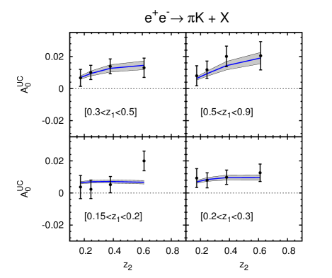
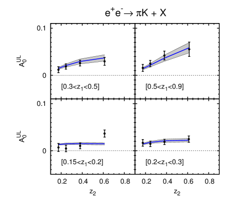
   Figure 1: The experimental data on the azimuthal correlations $A_{0}^{UC}$ and $A_{0}^{UL}$ as functions of $z_{1}$ and $z_{2}$ in unpolarised $e^{+}e^{-}\to\pi\,K\,X$ processes, as measured by the BaBar Collaboration, are compared to the curves obtained from our reference fit, given by the parameters shown in Eq. (26). The shaded area corresponds to the statistical uncertainty on these parameters.

   

   

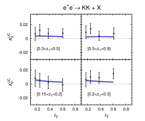
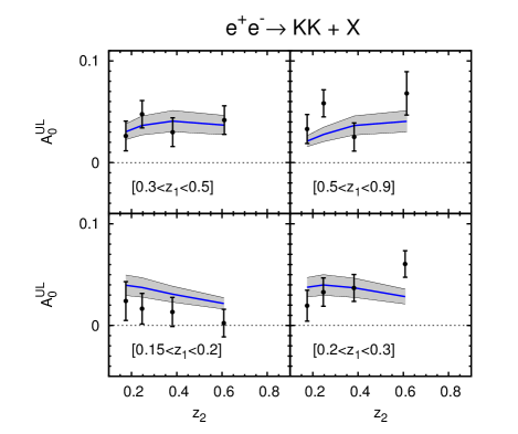
   Figure 2: The experimental data on the azimuthal correlations $A_{0}^{UC}$ and $A_{0}^{UL}$ as functions of $z_{1}$ and $z_{2}$ in unpolarised $e^{+}e^{-}\to K^{+}K^{-}\,X$ processes, as measured by the BaBar Collaboration, are compared to the curves obtained from our reference fit, given by the parameters shown in Eq. (26). The shaded area corresponds to the statistical uncertainty on these parameters.

3. We deliberately choose not to include SIDIS kaon data in the fit at this stage. Including them would, in principle, require a global analysis of both pion and kaon data sets which is beyond the scope of this paper. Moreover, we would like to test the universality of the Collins fragmentation functions in $e^{+}e^{-}$ and SIDIS, as proposed in Ref. Collins and Metz (2004), and check whether the kaon favoured and disfavoured Collins functions extracted from $e^{+}e^{-}$ annihilation data can describe the Collins asymmetries observed in SIDIS processes. We compute the Collins SIDIS asymmetry $A_{UT}^{\sin(\phi_{h}+\phi_{S})}$, using the kaon Collins functions given by our reference fit, Eqs. (8), (9) and (26), and the transversity distributions obtained in Ref. Anselmino et al. (2015) and given in Table 1. The comparison of our predictions with the measurements performed by the HERMES and COMPASS Collaborations is shown in Figs. 3 and 4 respectively. The good agreement confirms, within the precision limits of experimental data, the consistency of the Collins functions extracted from $e^{+}e^{-}$ data with those active in SIDIS processes.

   

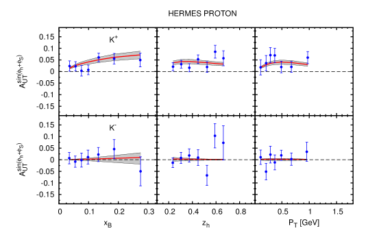
   Figure 3: The experimental data on the SIDIS azimuthal moment $A_{UT}^{\sin(\phi_{h}+\phi_{S})}$ as measured by the HERMES Collaboration Airapetian et al. (2010), are compared with our computation of the same quantity. The solid (red) lines correspond to our reference fit, with the parameters given in Eq. (26). The shaded area corresponds to the statistical uncertainty on these parameters. For the transversity distributions we used the fixed parameters reported in Table 1.

   

   

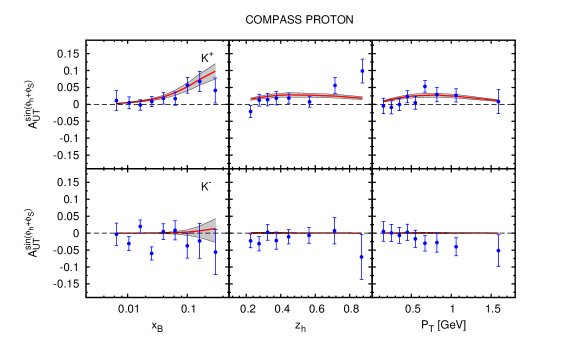
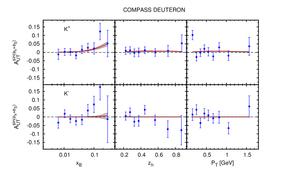
   Figure 4: The experimental data on the SIDIS Collins SSA $A_{UT}^{\sin(\phi_{h}+\phi_{S})}$ as measured by the COMPASS Collaboration on proton (upper panel) Adolph et al. (2015) and deuteron (lower panel) targets Alekseev et al. (2009), are compared with our computation of the same quantity. The solid (red) lines correspond to our reference fit, with the parameters given in Eq. (26). The shaded area corresponds to the statistical uncertainty on these parameters. For the transversity distributions we used the fixed parameters reported in Table 1.

III.1 Fits with additional parameters

Looking at the results of our reference fit, Eq. (26), the disfavoured Collins function appears to be quite undetermined and compatible with zero, while the favoured one is definitely non-zero and positive. However, we have assumed that the heavy ($s$ quark) and light ($u$ quark) favoured contributions are controlled by the same parameter. We wonder whether, by disentangling these two contributions, one can confirm the results obtained above.

An inspection of the analytical formulae, Eqs. (20), (21) and (14), (15), shows that the sign of the light-flavour favoured contribution is determined by the $\pi K$ data, where it appears convoluted with the pion Collins function, which is fixed. Most of the information, in particular, comes from the $A_{0}^{UL}$ asymmetries, which are dominated by doubly favoured terms of the type $\tilde{\Delta}^{N}D_{\pi^{+}/u^{\uparrow}}\tilde{\Delta}^{N}D_{K^{-}/{\bar{u}}^{\uparrow}}$.

The heavy flavour contribution, instead, is not determined by the data (not even in sign): this is due to the fact that, in $KK$ production processes, it appears in doubly favoured terms where it is convoluted with itself and therefore insensitive to the sign choice, while in $\pi K$ production processes it appears only in sub-leading combinations, such as $\tilde{\Delta}^{N}D_{\pi^{-}/s^{\uparrow}}\tilde{\Delta}^{N}D_{K^{+}/{\bar{s}}^{\uparrow}}$.

To study this in more detail, we have performed a series of fits allowing for up to three free parameters, i.e. one normalisation constant for the favoured light flavour, $N^{\rm light}_{\rm fav}$, one for the favoured heavy flavour, $N^{\rm heavy}_{\rm fav}$, and one for the disfavoured, $N_{\rm dis}$, contributions. The results, with the $\chi^{2}_{\rm d.o.f.}$ for each of the fits, are presented in Table 3, while some correlations between the parameters are studied in Fig. 5. Let us comment on such results.

• The first clear conclusion is that it is not possible to fit the data with one and only one of the parameters $N^{\rm light}_{\rm fav}$, $N^{\rm heavy}_{\rm fav}$, $N_{\rm dis}$, as shown in the upper panel of Table 3.

• Regarding the two parameter fits (central panel of Table 3), we see that the data can be successfully described only by including the light favoured contribution together with either the heavy favoured or the disfavoured Collins function. Notice that the sign of the heavy contribution, can be either positive or negative, leading to equally good fits (first two lines of the central panel in Table 3). The sign of $N_{\rm fav}^{\rm light}$ turns out to be always positive, with its best value in the approximate range between $0.3$ and $0.6$ (see the left panel of Fig. 5). Instead, fitting the data without any light quark favoured contribution appears not to be possible (last two lines of the central panel in Table 3).

• Fits with three parameters (bottom panel of Table 3) result in good values of $\chi^{2}_{\rm d.o.f.}$. These fits allow us to study the correlation among the free parameters. We, in fact, observe a very strong correlation between the heavy flavour (favoured) and the disfavoured contributions to the kaon Collins functions: values of $N^{\rm heavy}_{\rm fav}$ with opposite sign can easily be compensated by different values of $N_{\rm dis}$, resulting in fits of equal quality, as shown in the last part of Table 3. We actually find two distinct solutions resulting from the present data, one with positive and one with negative heavy flavour Collins FFs.

  Fig. 5 (right panel) illustrates this correlation. Two distinct distributions are clearly evident: red(blue) points represent solutions with positive(negative) $N^{\rm heavy}_{\rm fav}$. All points in the figure correspond to a total $\chi^{2}$ included between $\chi^{2}_{\rm min}$ and $\chi^{2}_{\rm min}+\Delta\chi^{2}$; for a three parameter fit $\Delta\chi^{2}=8.02$. The spread of the points indicates the statistical error which affects the two parameters. Lighter(darker) shades of color represent higher(lower) values of $\chi^{2}$. The points in which $\chi^{2}\equiv\chi^{2}_{\rm min}$ are shown as green squares.

  Notice that model calculations predict the same sign of light and heavy flavour Collins FF, see for instance Ref. Bacchetta et al. (2008).

In Fig. 6 we show the lowest $\mbox{\boldmath$p$}_{\perp}$-moment of the light-flavour favoured kaon Collins function, as extracted in our reference fit (with the parameters of Eq. (26)). Note that, in the case of a factorised Gaussian shape, Eqs. (3), (4) and (5), the lowest $\mbox{\boldmath$p$}_{\perp}$-moment of the Collins function,

$$\Delta^{N}D_{h/q^{\uparrow}}(z,Q^{2})=\int\,d^{2}\mbox{\boldmath$p$}_{\perp}\,\Delta^{N}D_{h/q^{\uparrow}}(z,p_{\perp},Q^{2})\,,$$ (27)

is related to the $z$-dependent part of the Collins function, $\tilde{\Delta}^{N}D_{h/q^{\uparrow}}(z,Q^{2})$, by

$$\Delta^{N}D_{h/q^{\uparrow}}(z,Q^{2})=\frac{\sqrt{\pi}}{2}\,\frac{\langle p_{\perp}^{2}\rangle_{{}_{\!C}}^{3/2}}{\langle p_{\perp}^{2}\rangle}\,\frac{\sqrt{2e}}{M_{C}}\,\tilde{\Delta}^{N}D_{h/q^{\uparrow}}(z,Q^{2})\,.$$ (28)

The heavy flavour favoured and (all flavour) disfavoured results are not shown: in fact, the study performed above shows that it is not possible to reliably distinguish between these two contributions to the available data. Furthermore, not even the sign of the heavy flavour favoured Collins function can be determined.

$N_{\rm fav}^{\rm light}$	$N_{\rm fav}^{\rm heavy}>0$	$N_{\rm fav}^{\rm heavy}<0$	$N_{\rm dis}$	$\chi^{2}_{\rm d.o.f.}$
•	◦	◦	◦	1.83
◦	•	◦	◦	3.32
◦	◦	•	◦	5.68
◦	◦	◦	•	3.94
•	•	◦	◦	0.89
•	◦	•	◦	0.88
•	◦	◦	•	0.98
◦	•	◦	•	2.00
◦	◦	•	•	4.00
•	•	◦	•	0.90
•	◦	•	•	0.89

Table 3: $\chi^{2}$/d.o.f. for different scenarios for the kaon Collins functions: one-parameter (upper panel), two-parameter (central panel) and three-parameter (lower panel) fits. The symbol • means that the corresponding parameter is actually used in the fit, while the symbol ◦ means that the contribution to the Collins asymmetry corresponding to that parameter is not included in the fit. For $N_{\rm fav}^{\rm heavy}$, we explicitly indicate the two different constraints we use: $N_{\rm fav}^{\rm heavy}>0$ and $N_{\rm fav}^{\rm heavy}<0$.

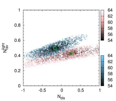
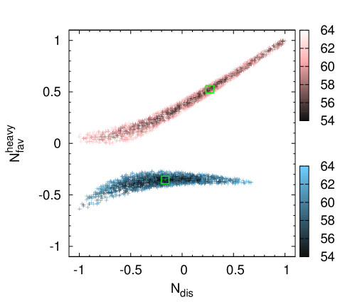
Figure 5: Correlation between the parameters: $N^{\rm light}_{\rm fav}$ and $N_{\rm dis}$ (left panel) and $N^{\rm heavy}_{\rm fav}$ and $N_{\rm dis}$ (right panel). Red points represent solutions with positive $N^{\rm heavy}_{\rm fav}$, while blue points represent solutions with negative $N^{\rm heavy}_{\rm fav}$. All points in the figure correspond to a total $\chi^{2}$ included between $\chi^{2}_{\rm min}$ and $\chi^{2}_{\rm min}+\Delta\chi^{2}$; the spread of the points indicates the statistical error which affects the two parameters. Lighter(darker) shades of color represent higher(lower) values of $\chi^{2}$. The points in which $\chi^{2}\equiv\chi^{2}_{\rm min}$ are shown as green squares.

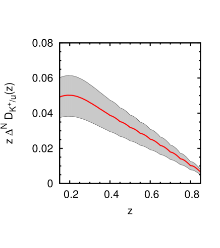
Figure 6: Plot of $z$ times the lowest $\mbox{\boldmath$p$}_{\perp}$-moment, Eqs. (27) and (28), of the $u^{\uparrow}\to K^{+}\,X$ Collins function, as extracted in our reference fit (with the parameters of Eq. (26)). The analogous plots for heavy flavour favoured and (all flavour) disfavoured Collins functions are not shown: in fact, it is not possible to reliably distinguish between these two contributions to the available BaBar data. Furthermore, not even the sign of the heavy flavour favoured Collins function can be determined.

IV Comments and conclusions

We have extracted, for the first time, the kaon Collins functions, $q^{\uparrow}\to K\,X$, by best fitting recent BaBar data Aubert et al. (2015). This paper extends a recent study of the Collins functions in $e^{+}e^{-}$ and SIDIS processes Anselmino et al. (2015) limited to pion production.

It turns out that a simple phenomenological parameterisation of the Collins function, Eqs. (3) and (4), is quite adequate to describe the data. When comparing with the pion Collins functions Anselmino et al. (2015), due to the limited amount and relatively big errors of data, an even smaller number of parameters suffices to describe the experimental results. Indeed, we find that kaon Collins functions of two kinds, favoured and disfavoured, both simply proportional to the unpolarised TMD fragmentation functions, describe well the BaBar data.

As a result of the attempted fits, we can conclude that a definite outcome of this study is the determination of a positive $u^{\uparrow}\to K^{+}X=\bar{u}^{\uparrow}\to K^{-}X$ Collins function, assuming a positive favoured pion Collins function Anselmino et al. (2015). No definite independent conclusion, based on the available data, can be drawn on the signs of $s^{\uparrow}\to K^{-}X=\bar{s}^{\uparrow}\to K^{+}X$ Collins functions and on the disfavoured ones.

The extracted kaon Collins functions, together with the transversity distributions obtained in Ref. Anselmino et al. (2015), give a very good description, within the rather large experimental uncertainties, of SIDIS data on kaon Collins asymmetries measured by COMPASS Adolph et al. (2015); Alekseev et al. (2009) and HERMES Airapetian et al. (2010) Collaborations. This points towards a consistent and universal role of the Collins effect in different physical processes, which should be further explored in the future.

References

Anselmino et al. (2007)
M. Anselmino,
M. Boglione,
U. D’Alesio,
A. Kotzinian,
F. Murgia,
et al., Phys. Rev.
D75, 054032
(2007), eprint hep-ph/0701006.
Anselmino et al. (2009)
M. Anselmino,
M. Boglione,
U. D’Alesio,
A. Kotzinian,
F. Murgia,
et al., Nucl. Phys. Proc. Suppl.
191, 98 (2009),
eprint 0812.4366.
Anselmino et al. (2013)
M. Anselmino,
M. Boglione,
U. D’Alesio,
S. Melis,
F. Murgia,
et al., Phys. Rev.
D87, 094019
(2013), eprint 1303.3822.
Anselmino et al. (2015)
M. Anselmino,
M. Boglione,
U. D’Alesio,
J. O. G. Hernandez,
S. Melis,
F. Murgia, and
A. Prokudin
(2015), eprint 1510.05389.
Airapetian et al. (2010)
A. Airapetian
et al. (HERMES Collaboration),
Phys. Lett. B693,
11 (2010), eprint 1006.4221.
Airapetian et al. (2013)
A. Airapetian
et al. (HERMES Collaboration),
Phys. Rev. D87,
012010 (2013), eprint 1204.4161.
Alekseev et al. (2009)
M. Alekseev et al.
(COMPASS Collaboration), Phys.
Lett. B673, 127
(2009), eprint 0802.2160.
Adolph et al. (2015)
C. Adolph et al.
(COMPASS Collaboration), Phys.
Lett. B744, 250
(2015), eprint 1408.4405.
Aubert et al. (2015)
B. Aubert et al.
(BaBar Collaboration) (2015),
eprint 1506.05864.
Collins and Metz (2004)
J. C. Collins and
A. Metz,
Phys. Rev. Lett. 93,
252001 (2004), eprint hep-ph/0408249.
Anselmino et al. (2014)
M. Anselmino,
M. Boglione,
J. Gonzalez Hernandez,
S. Melis, and
A. Prokudin,
JHEP 1404, 005
(2014), eprint 1312.6261.
Gluck et al. (1998)
M. Gluck,
E. Reya, and
A. Vogt,
Eur.Phys.J. C5,
461 (1998), eprint hep-ph/9806404.
de Florian et al. (2007)
D. de Florian,
R. Sassot, and
M. Stratmann,
Phys.Rev. D76,
074033 (2007), eprint 0707.1506.
Lees et al. (2014)
J. Lees et al.
(BaBar Collaboration), Phys.Rev.
D90, 052003
(2014), eprint 1309.5278.
Seidl et al. (2008)
R. Seidl et al.
(Belle Collaboration), Phys. Rev.
D78, 032011
(2008), eprint 0805.2975.
Seidl et al. (2012)
R. Seidl et al.
(Belle Collaboration), Phys. Rev.
D86, 032011(E)
(2012), eprint 0805.2975.
Bacchetta et al. (2008)
A. Bacchetta,
L. P. Gamberg,
G. R. Goldstein,
and
A. Mukherjee,
Phys. Lett. B659,
234 (2008), eprint 0707.3372.