Unitary rotation and gyration
of pixellated images on rectangular screens

Abstract

In the two space dimensions of screens in optical systems, rotations, gyrations, and fractional Fourier transformations form the Fourier subgroup of the symplectic group of linear canonical transformations: $\hbox{\sf U($2$)}_{\scriptscriptstyle\rm F}\subset\hbox{\sf Sp($4$,R)}$. Here we study the action of this Fourier group on pixellated images within generic rectangular $N_{x}\times N_{y}$ screens; its elements here compose properly and act unitarily, i.e., without loss of information.

1 Introduction

Paraxial geometric, wave, and finite optical models with two-dimensional plane screens, are covariant with the Fourier group $\hbox{\sf U($2$)}_{\scriptscriptstyle\rm F}$. This group consists of joint SO($2$) phase space rotations between the coordinates ${\bf q}=(q_{x},q_{y})$ and between their canonically conjugate momenta ${\bf p}=(p_{x},p_{y})$; also it contains joint SO($2$) gyrations in the $(q_{x},p_{y})$ and $(q_{y},p_{x})$ planes; and finally, of $\hbox{\sf SO($2$)}_{x}\otimes\hbox{\sf SO($2$)}_{y}$ fractional Fourier transformations that rotate independently the $(q_{x},p_{x})$ and $(q_{y},p_{y})$ planes, and all their compositions. In the geometric model, the group $\hbox{\sf U($2$)}_{\scriptscriptstyle\rm F}$ is represented by $4\times 4$ matrices that are both orthogonal and symplectic [1]; in the wave model of images on the screen, $f(q_{x},q_{y})$, ${\bf q}\in{\sf R}^{2}$, these are subject to integral linear canonical transforms [2, 3] that represent this same group. In the finite model of optics, where images are matrices of values $f(q_{x},q_{y})$, the coordinates $q_{x},\,q_{y}$ are integers that count the $N_{x}\times N_{y}$ pixels in a rectangular screen, so the Fourier group will be represented by square $N_{x}N_{y}\times N_{x}N_{y}$ matrices that are unitary. Of course, being elements of a group, these $\hbox{\sf U($2$)}_{\scriptscriptstyle\rm F}$ transformations can be concatenated and inverted using their simplest $4\times 4$ representation.

Previously we have considered the action of the $\hbox{\sf U($2$)}_{\scriptscriptstyle\rm F}$ Fourier group on finite systems, where the screens were $N{\times}N$ squares [4, 5, 6]. The extension to rectangular screens where $N_{x}\neq N_{y}$, is not trivial because rotations and gyrations to “angular momentum” Laguerre-type modes require an extended form of symmetry importation [7, 8].

In Sects. 2 and 3 we recall the foundations of the finite model of pixellated optics and the definition of the Fourier group in the paraxial geometric model. The fractional Fourier transforms have their corresponding matrix Fourier-Kravchuk transform [9] within the finite model, i.e., they are domestic to it. Rotations and gyrations however, require importation from the geometric model; this is done in Sect. 4, where we provide computed examples of these transformations and show the finite rectangular analogues of the Laguerre-Gauss modes of wave optics [10]. In Sect. 5 we offer some concluding remarks on applications to image processing.

2 Continuous and finite oscillator systems

The linear finite oscillator system arises as the algebra and group deformation of the well-known quantum harmonic oscillator, upon which the continuous position and momentum coordinates become discrete and finite.

Let $\bar{Q},\,\bar{P}$ and $\bar{H}:={\textstyle\frac{1}{2}}(\bar{P}^{2}+\bar{Q}^{2}-{\it 1})$ be the Poisson-bracket or the Schrödinger operators of position, momentum and mode number (do not confuse with the Hamiltonian, which is $\bar{H}+{\textstyle\frac{1}{2}}{\it 1})$, indicating by the over-bar that they refer to the continuous model. On the other hand, consider the three components of quantum angular momentum, designated by the letters $Q\equiv J_{1}$, $P\equiv-J_{2}$ and $K\equiv J_{3}$, and compare their well-known commutation relations that characterize the oscillator and spin algebras,

$$\begin{array}[]{rlll}\hbox{\sf osc}_{1}:&[\bar{H},\bar{Q}]=-{\rm i}\bar{P},&[\bar{H},\bar{P}]=+{\rm i}\bar{Q},&[\bar{Q},\par P]={\rm i}\eta{\it 1};\\ \hbox{\sf su($2$)}:&[K,Q]=-{\rm i}P,&[K,P]=+{\rm i}Q,&[Q,P]=-{\rm i}K.\end{array}$$ (1)

The first two commutators in each line are the algebraic form of the geometric and dynamical Hamilton equations for the harmonic oscillator in phase space, under evolution by $\bar{H}$ and $K$ respectively. The last two commutators however differ, and distinguish between the continuous and the finite models: in their unitary irreducible representations, the $\hbox{\sf osc}_{1}$ spectrum of $\bar{Q}$ and $\bar{P}$ is continuous and fills the real line $\sf R$ while that of $\bar{H}$ is the equally-spaced set $\eta n$ ($\eta$ fixed) with $n|_{0}^{\infty}$ integer; the spectrum of the three su($2$) generators on the other hand, in the representation $j$ (positive integer or half-integer determined by the eigenvalue $j(j{+}1)$ of the Casimir invariant $\vec{J}\cdot\vec{J}\,$), is the unit-spaced set $m|_{-j}^{j}$. This leads us to understand $K+j{\it 1}$ as the mode number operator of a discrete oscillator system that has $2j+1$ modes $n|_{0}^{2j}$.

The oscillator Lie algebra $\hbox{\sf osc}_{1}$ of generators ${\it 1},\,\bar{Q},\,\bar{P},\,\bar{H}$ is the contraction of the algebra $\hbox{\sf u($2$)}=\hbox{\sf u($1$)}\oplus\hbox{\sf su($2$)}$ with generators ${\it 1},\,Q,\,P,\,K$, when we let $j\to\infty$ as the number and density of discrete points grows without bound [11]. This u($2$) can be called the mother algebra of the finite oscillator model. The wavefunctions in each model are the overlaps between the eigenfunctions of their mode generator and their position generator; they are the Hermite-Gauss (HG) functions $\Psi_{n}^{\scriptscriptstyle\rm HG}(q)$ in the continuous model, and Kravchuk functions on the discrete position points of the finite model, given by quantum angular momentum theory as Wigner little-d functions [12, 13], for the angle ${\textstyle\frac{1}{2}}\pi$ between $J_{1}$ and $J_{3}$,

$$\begin{array}[]{rcl}\Psi_{n}^{(j)}(q)&:=&d^{j}_{n-j,q}({\textstyle\frac{1}{2}}\pi)\\[3.0pt] &=&\displaystyle\frac{(-1)^{n}}{2^{j}}\sqrt{\Big{(}{2j\atop n}\Big{)}\Big{(}{2j\atop j{+}q}\Big{)}}\,K_{n}(j{+}q;\,{\textstyle\frac{1}{2}},2j),\\[10.0pt] K_{n}(s;{\textstyle\frac{1}{2}},2j)&=&{}_{2}F_{1}(-n,-s;-2j;2)=K_{s}(n;{\textstyle\frac{1}{2}},2j),\end{array}$$ (2)

where $s|_{0}^{2j}$, $n|_{0}^{2j}$, $q|_{-j}^{j}$, $K_{n}(s;{\textstyle\frac{1}{2}},2j)$ is a symmetric Kravchuk polynomial [14], and ${}_{2}F_{1}(a,b;c;z)$ is the Gauss hypergeometric function. These functions form multiplets under su($2$) that have been detailed in several papers [9, 15], where they are shown to possess the desirable properties of the continuous $HG$ modes. For the lowest $n$’s, the points $\Psi_{n}^{(j)}(q)$ fall closely on the continuous $\Psi_{n}^{\scriptscriptstyle\rm HG}(q)$, while for higher $n$’s, they alternate in sign between every pair of neighbour points,

$$\Psi_{2j-n}^{(j)}(q)=(-1)^{q}\Psi_{n}^{(j)}(q).$$ (3)

3 The Fourier algebra and group

Consider now two space dimensions $k\in\{x,y\}$, the two momentum operators, the corresponding two independent mode operators, and the single 1 (with $\eta_{k}=1$). The $\hbox{\sf osc}_{2}$ Lie algebra thus generalizes (1) to

$$\begin{array}[]{c}[\bar{H}_{k},\bar{Q}_{k^{\prime}}]=-{\rm i}\delta_{k,k^{\prime}}\bar{P}_{k},\quad[\bar{H}_{k},\bar{P}_{k^{\prime}}]={\rm i}\delta_{k,k^{\prime}}\bar{Q}_{k},\\[5.0pt] \displaystyle[\bar{Q}_{k},\bar{P}_{k^{\prime}}]={\rm i}\delta_{k,k^{\prime}}{\it 1},\end{array}$$ (4)

plus $[\bar{Q}_{k},\bar{Q}_{k^{\prime}}]=0$ and $[\bar{P}_{k},\bar{P}_{k^{\prime}}]=0$.

Out of all quadratic products of $\bar{Q}_{k}$ and $\bar{P}_{k^{\prime}}$, one obtains the 10 generators of the symplectic real Lie algebra sp($4$,R) of paraxial optics, whose maximal compact subalgebra is the Fourier algebra $\hbox{\sf u($2$)}_{\scriptscriptstyle\rm F}$ [1]. This algebra contains four up-to second degree differential operators that we identify as the generators of Fourier transformations (FT’s) and other phase space rotations,

$$\hbox{symmetric FT }\bar{L}_{0} := {\textstyle\frac{1}{4}}(\bar{P}_{x}^{2}{+}\bar{P}_{y}^{2}{+}\bar{Q}_{x}^{2}{+}\bar{Q}_{y}^{2}{-}2{\it 1})$$ (5)

$$= {\textstyle\frac{1}{2}}(\bar{H}_{x}{+}\bar{H}_{y}),$$

$${}\!\!\!\!\!\!\hbox{antisymmetric FT }\bar{L}_{1} := {\textstyle\frac{1}{4}}(\bar{P}_{x}^{2}{-}\bar{P}_{y}^{2}{+}\bar{Q}_{x}^{2}{-}\bar{Q}_{y}^{2})$$ (6)

$$= {\textstyle\frac{1}{2}}(\bar{H}_{x}{-}\bar{H}_{y}),$$

$$\hbox{gyration }\bar{L}_{2} := {\textstyle\frac{1}{2}}(\bar{P}_{x}\bar{P}_{y}+\bar{Q}_{x}\bar{Q}_{y}),$$ (7)

$$\hbox{rotation }\bar{L}_{3} := {\textstyle\frac{1}{2}}(\bar{Q}_{x}\bar{P}_{y}-\bar{Q}_{y}\bar{P}_{x})=:{\textstyle\frac{1}{2}}\bar{M},$$ (8)

where $\bar{M}=2\bar{L}_{3}$ is the physical angular momentum operator. Their commutation relations are

$$[\bar{L}_{0},\bar{L}_{\ell}]=0,\quad[\bar{L}_{i},\,\bar{L}_{j}]={\rm i}\,\bar{L}_{\ell},$$ (9)

where the indices $i,\,j,\,\ell$ are a cyclic permutation of $1,\,2,\,3$. Abstractly, (6)–(8) generate rotations of a 2-sphere.

For the finite oscillator model in two dimensions we consider the direct sum of two su($2$) algebras, whose generators form a vector basis for ${\hbox{\sf su($2$)}}_{x}\oplus{\hbox{\sf su($2$)}}_{y}$, which is (accidentally) homomorphic to the four-dimensional rotation algebra so($4$) [12]. We choose the representation of this algebra to be $(j_{x},j_{y})$, determined by the values of the two independent Casimir operators in ${\hbox{\sf su($2$)}}_{x}\oplus{\hbox{\sf su($2$)}}_{y}$. The spectra of positions in the $x$- and $y$-directions will thus be $q_{k}|_{-j_{k}}^{j_{k}}$, as will the corresponding spectra of momenta, and modes are numbered by $n_{k}|_{0}^{2j_{k}}$. We interpret the positions as the coordinates of pixels or points in an $N_{x}\times N_{y}=(2j_{x}{+}1)\times(2j_{y}{+}1)$ rectangular array. The two-dimensional finite harmonic oscillator functions are real and the Cartesian products of Kravchuk functions (2) in the two coordinates are [4],

$$\begin{array}[]{r}\Psi_{n_{x},n_{y}}^{(j_{x},j_{y})}(q_{x},q_{y}):=\Psi_{n_{x}}^{(j_{x})}(q_{x})\Psi_{n_{y}}^{(j_{y})}(q_{y}),\\ q_{x}|_{-j_{x}}^{j_{x}},\ n_{x}|_{0}^{2j_{x}},\ q_{y}|_{-j_{y}}^{j_{y}},\ n_{y}|_{0}^{2j_{y}}.\end{array}$$ (10)

There are thus $N_{x}N_{y}$ two-dimensional Kravchuk functions that can be arranged along axes of total mode $n:=n_{x}+n_{y}$ and $m:=n_{x}-n_{y}$ into the rhomboid pattern shown in Fig. 1. As eigenvectors of commuting operators in the Lie algebra, the Cartesian modes (10) are orthonormal and complete under the natural inner product,

$${}\!\!\!\!\!\!\!\!\!\sum_{n_{x},n_{y}}\!\!\Psi_{n_{x},n_{y}}^{(j_{x},j_{y})}(q_{x},q_{y})^{*}\Psi_{n_{x},n_{y}}^{(j_{x},j_{y})}(q^{\prime}_{x},q^{\prime}_{y}) = \delta_{q_{x},q^{\prime}_{x}}\delta_{q_{y},q^{\prime}_{y}},$$ (11)

$${}\!\!\!\!\!\!\!\!\!\sum_{q_{x},q_{y}}\!\!\Psi_{n_{x},n_{y}}^{(j_{x},j_{y})}(q_{x},q_{y})^{*}\Psi_{n^{\prime}_{x},n^{\prime}_{y}}^{(j_{x},j_{y})}(q_{x},q_{y}) = \delta_{n_{x},n^{\prime}_{x}}\delta_{n_{y},n^{\prime}_{y}}.$$ (12)

We shall assume throughout that $j_{x}>j_{y}$; when $j_{x}=j_{y}$ there will be evident simplifications.

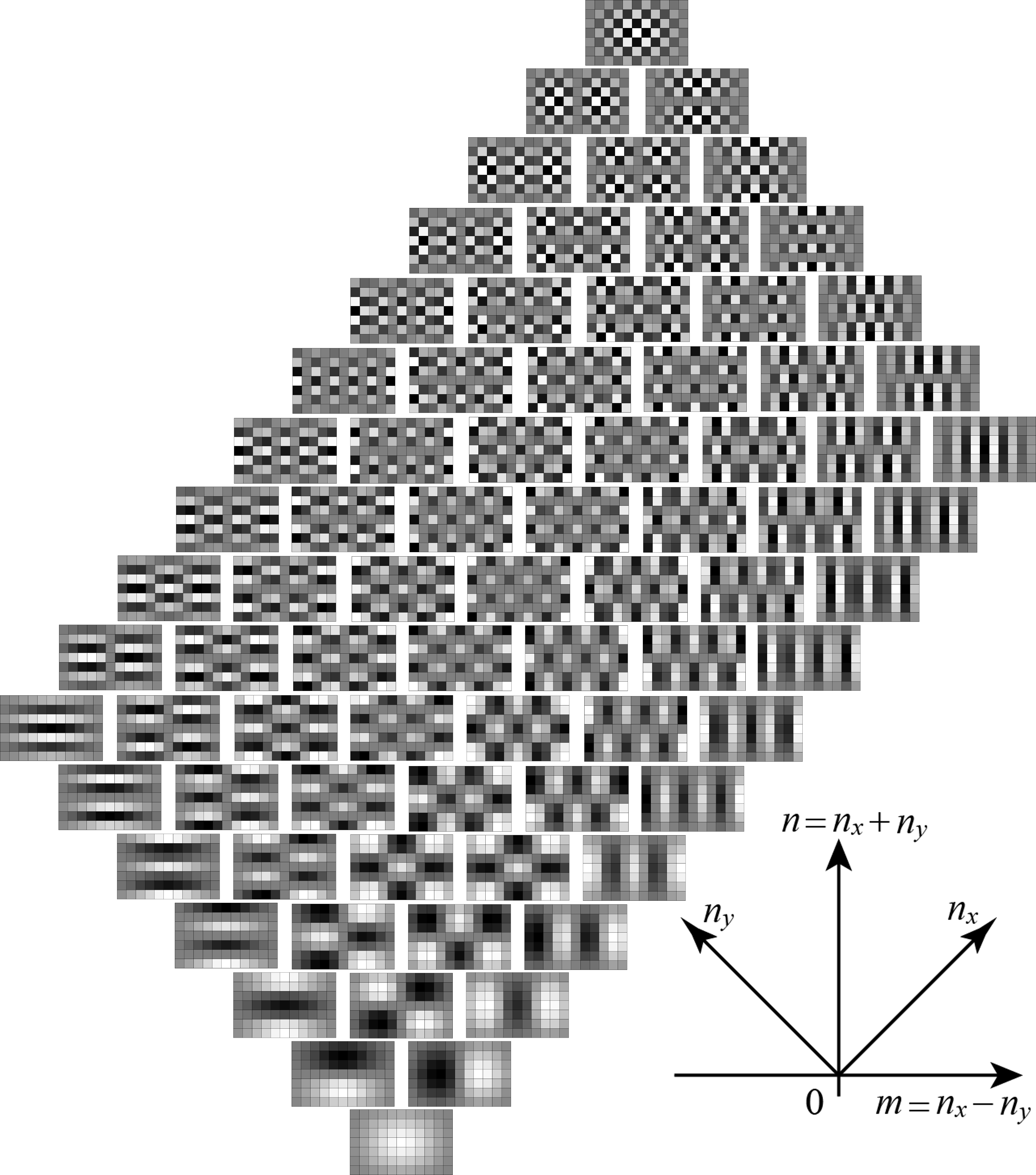
Figure 1: Rhomboid with the $11\times 7$ Cartesian modes $\Psi_{n_{x},n_{y}}^{(5,3)}(q_{x},q_{y})$ in (10), arranged by $n_{x}|_{0}^{10},\,n_{y}|_{0}^{6}$ and also referred to the axes of total mode $n=n_{x}+n_{y}$ and ‘angular momentum’ $m=n_{x}-n_{y}$. In each mode, the pixels are numerated by $q_{x}|_{-5}^{5},\,q_{y}|_{-3}^{3}$, where the $(q_{x},q_{y})=(5,3)$ pixels are in the upper-right corners. The range of grey-level densities, from black to white, is $(-1,1)$

Among the Cartesian modes $\Psi_{n_{x},n_{y}}^{(j_{x},j_{y})}(q_{x},q_{y})$ in (10) and Fig. 1 we note that in the lower triangle, where $0\leq n\leq 2j_{y}<2j_{x}$, the right and left extremes of each $n={}$constant row exhibit $n_{x}$ and $n_{y}$ nodes (changes of sign between pixel neighbours) respectively, both of which can be accommodated within the pixels of the $N_{x}$ columns and $N_{y}$ rows. As we enter the middle rhomboid, where $2j_{y}<n<2j_{x}$, the right extreme $n_{x}=n\leq N_{x}-1$ can accomodate its vertical nodes within the horizontal length of the screen, but its left extreme cannot do so among its $N_{y}$ rows, so only $N_{y}-1$ nodes become horizontal while the rest must remain vertical. Finally in the upper triangle, where $2j_{x}\leq n\leq 2(j_{x}{+}j_{y})$, there will be both vertical as well as horizontal nodes in all modes. From (3) it follows that

$$\Psi_{2j_{x}-n_{x},2j_{y}-n_{y}}^{(j_{x},j_{y})}(q_{x},q_{y})=(-1)^{q_{x}+q_{y}}\Psi_{n_{x},n_{y}}^{(j_{x},j_{y})}(q_{x},q_{y}),$$ (13)

so that the upper triangle reproduces (top $\leftrightarrow$ bottom, left $\leftrightarrow$ right) the modes of the lower triangle, but superposed with a checkerboard of changes of sign.

The images on the $N_{x}\times N_{y}$ pixellated screen are value arrays $F(q_{x},q_{y})$ that can be expanded in terms of the set of Cartesian modes (10) as

$$\begin{array}[]{rcl}F(q_{x},q_{y})&=&\displaystyle\sum_{n_{x},n_{y}}F_{n_{x},n_{y}}\Psi_{n_{x},n_{y}}^{(j_{x},j_{y})}(q_{x},q_{y}),\\ F_{n_{x},n_{y}}&=&\displaystyle\sum_{q_{x},q_{y}}F(q_{x},q_{y})\,\Psi_{n_{x},n_{y}}^{(j_{x},j_{y})}(q_{x},q_{y}),\end{array}$$ (14)

as follows directly from linearity, and the orthonormality and completeness of the Kravchuk basis.

4 Importation of symmetry

In the continuous case, the two-dimensional harmonic oscillator mode functions $\Psi_{n_{x}}^{\scriptscriptstyle\rm HG}(q_{x})\*\Psi_{n_{y}}^{\scriptscriptstyle\rm HG}(q_{y})$ can be arranged in a pattern similar to Fig. 1 but without an upper bound, forming an ‘inverted tower’ with the same lower apex, out of which the total mode number $n:=n_{x}+n_{y}$ can grow indefinitely. Since $\bar{L}_{0}$ commutes with all generators in (5)–(8) of the $\hbox{\sf u($2$)}_{\scriptscriptstyle\rm F}$ algebra, functions with the same total mode number $n$ will transform among themselves under the whole Fourier $\hbox{\sf U($2$)}_{\scriptscriptstyle\rm F}$ group. Functions with same total mode number $n$ form su($2$) multiplets where the range of $n_{x}-n_{y}=:m|_{-n}^{n}$ is spaced by two units. This is equivalent to have multiplets of spin $\lambda:={\textstyle\frac{1}{2}}n$, with $\mu:={\textstyle\frac{1}{2}}m$ playing the role of angular momentum projection on a ‘3’-axis.

In the finite model however, the generators of the algebra $\hbox{\sf su($2$)}_{x}\oplus\hbox{\sf su($2$)}_{y}$ can raise and lower the modes only along the $n_{x}$ or $n_{y}$ directions of Fig. 1, but not horizontally, i.e., from one value of $\mu={\textstyle\frac{1}{2}}(n_{x}-n_{y})$ to its neighbours. Symmetry importation consists in defining linear transformations among the states of the finite system using the linear combination coefficients provided by continuous models [7, 8].

4.1 Rotations

The ‘physical’ angular momentum operator $\bar{M}$ in (8) generates rotations $\bar{\cal R}(\theta):=\exp(-{\rm i}\theta\bar{M})$ in the continuous model; this we now import to the finite model by simply eliminating the over-bar in the notation. So, because $M=2L_{3}$, ${\cal R}(\theta)$ is a rotation around the ‘3’-axis of the sphere by the double angle $2\theta$. Since the eigenvalues of $L_{0}$, $\lambda:={\textstyle\frac{1}{2}}n={\textstyle\frac{1}{2}}(n_{x}{+}n_{y})$, are invariant under ${\cal R}(\theta)$, the $2\lambda+1$ eigenstates of $L_{1}$, characterized by the difference eigenvalues $\mu:={\textstyle\frac{1}{2}}(n_{x}-n_{y})$, will mix with linear combination coefficients given by Wigner little-$d$ functions $d_{\mu,\mu^{\prime}}^{\lambda}(2\theta)$ [5, 12, 15]. (Note that the usual 1-2-3 numbering of axes is rotated to 2-3-1.)

To act on the Cartesian finite oscillator states $\Psi_{n_{x},n_{y}}^{(j_{x},j_{y})}(q_{x},q_{y})$ in (10), we note the shape of the rhomboid in Fig. 1, and define their rotation (initially as a conjecture) by

$${\cal R}(\theta):\Psi_{n_{x},n_{y}}^{(j_{x},j_{y})}(q_{x},q_{y}):=\!\!\!\!\!\!\sum_{n^{\prime}_{x}+n^{\prime}_{y}=n}\!\!\!\!\!\!d^{\lambda(n)}_{\mu,\mu^{\prime}}(2\theta)\Psi_{n^{\prime}_{x},n^{\prime}_{y}}^{(j_{x},j_{y})}(q_{x},q_{y}),$$ (15)

where the values of spin $\lambda=\lambda(n)$ and their projections $\mu(j_{x},j_{y};n_{x},n_{y})$ must now be examined with some care. The rhomboid contains three distinct intervals of $n$ that should agree with the correct angular momentum $\lambda$ of all imported su($2$) multiplets in the horizontal rows of Fig. 1.

As we have assumed $j_{x}>j_{y}$, we recognize that in each of the three intervals $\lambda(n)$ will be:

$$\begin{array}[]{lll}\begin{array}[]{l}\hbox{lower triangle:}\\ 0\leq n\leq 2j_{y},\end{array}&\left\{\begin{array}[]{l}\lambda(n)={\textstyle\frac{1}{2}}n,\\ \mu={\textstyle\frac{1}{2}}(n_{x}-n_{y}),\\ \mu^{\prime}={\textstyle\frac{1}{2}}(n^{\prime}_{x}-n^{\prime}_{y}),\end{array}\right.\\[15.0pt] \begin{array}[]{l}\hbox{mid rhomboid:}\\ 2j_{y}<n<2j_{x},\end{array}&\left\{\begin{array}[]{l}\lambda(n)=j_{y},\\ \mu=j_{y}-n_{y},\\ \mu^{\prime}=j_{y}-n^{\prime}_{y},\end{array}\right.\\[15.0pt] \begin{array}[]{l}\hbox{upper triangle:}\\ 2j_{x}\leq n\leq 2(j_{x}{+}j_{y}),\end{array}&\left\{\begin{array}[]{l}\lambda(n)=j_{x}{+}j_{y}{-}{\textstyle\frac{1}{2}}n,\\ \mu={\textstyle\frac{1}{2}}(n_{x}{-}n_{y}){-}j_{x}{+}j_{y},\\ \mu^{\prime}={\textstyle\frac{1}{2}}(n^{\prime}_{x}{-}n^{\prime}_{y}){-}j_{x}{+}j_{y}.\end{array}\right.\end{array}$$ (16)

The first two cases actually overlap for $n=2j_{y}$ and the second two cases for $n=2j_{x}$, which we adjudicate to the triangles (when $j_{x}=j_{y}$ only the two triangles are present [4] and overlap for $n=2j$). The rotation of various multiplets of two-dimensional Kravchuk modes are shown in Figs. 2.

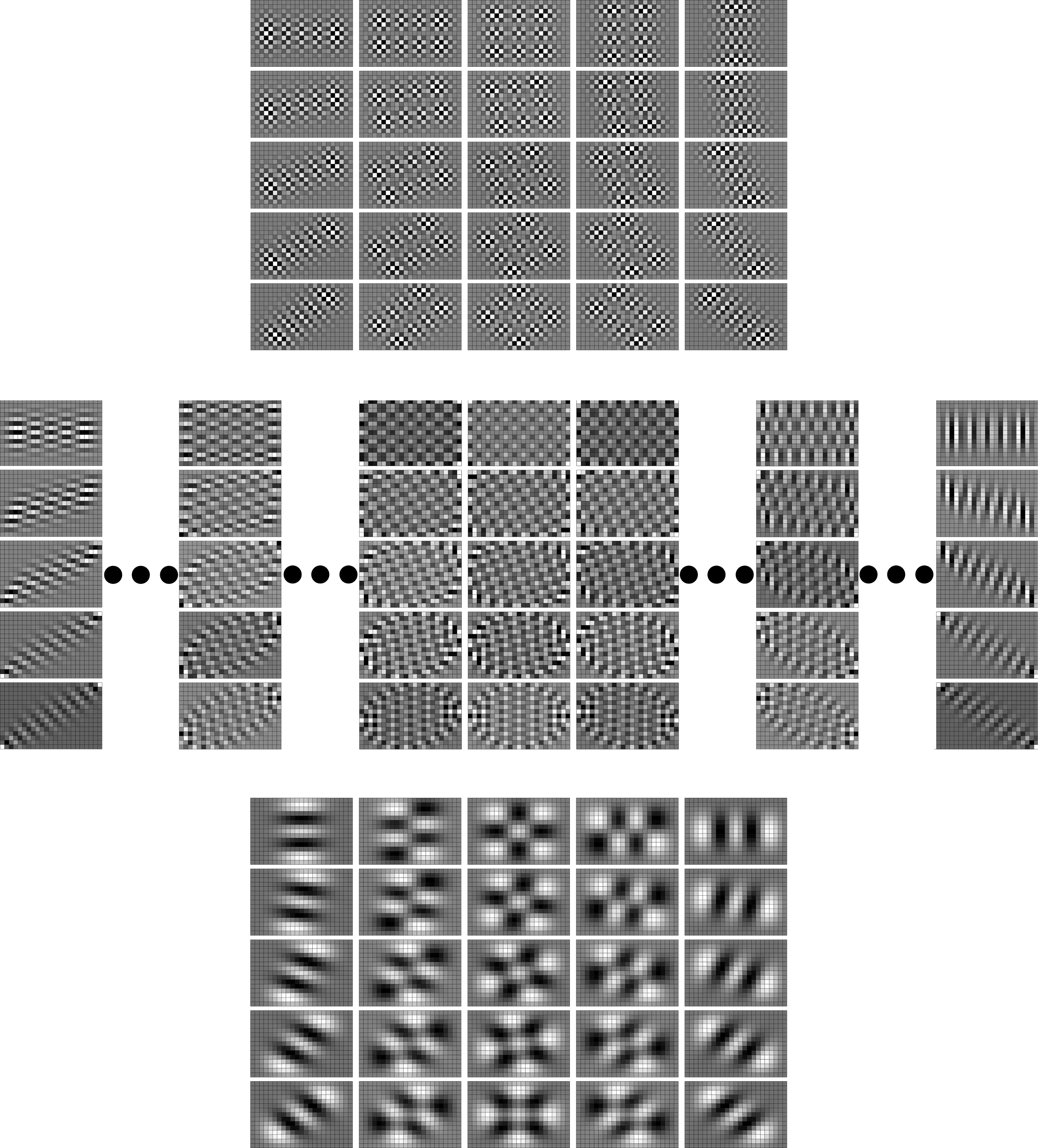
Figure 2: Rotations by $\theta=0$, $\frac{1}{4}\pi$, and $\frac{1}{2}\pi$, of selected Cartesian Kravchuk modes $\Psi_{n_{x},n_{y}}^{(11,7)}(q_{x},q_{y})$ in (15)–(16). Bottom: the 5 states of the level $n=4$ ($\lambda=2$) in the lower triangle. Middle: 5 selected states of the level $n=18$ ($\lambda=7$) in the mid rhomboid. Top: the 5 states of the level $n=32$ ($\lambda=2$). See that all rotate in the same direction.

The rotation of the pixellated images $F(q_{x},q_{y})$ on the $(2j_{x}{+}1)\times(2j_{y}{+}1)$ screen follows from (14) and the rotation (15) of the Cartesian basis,

$$\begin{array}[]{rcl}{\cal R}(\theta)\,{:}\,F(q_{x},q_{y})\!&=&\displaystyle\!\!\!\sum_{n_{x},n_{y}}\!F^{(\theta)}_{n_{x},n_{y}}\Psi_{n_{x},n_{y}}^{(j_{x},j_{y})}(q_{x},q_{y}),\\ F^{(\theta)}_{n_{x},n_{y}}\!&=&\displaystyle\!\!\!\sum_{q_{x},q_{y}}\!F(q_{x},q_{y})\,{\cal R}(\theta)\,{:}\,\Psi_{n_{x},n_{y}}^{(j_{x},j_{y})}(q_{x},q_{y})\end{array}$$ (17)

In Fig. 3 we show the rotation of a white on black (1’s on 0’s) image of the letter “F”. We note the inevitable ‘Gibbs’ oscillations around the sharp edges of the figure; yet we should stress that the rotated images were obtained by successive rotations of $\frac{1}{6}\pi$. The reconstruction of the original image after six rotations by $\frac{1}{6}\pi$ would be impossible with any interpolation algorithm applied successively.

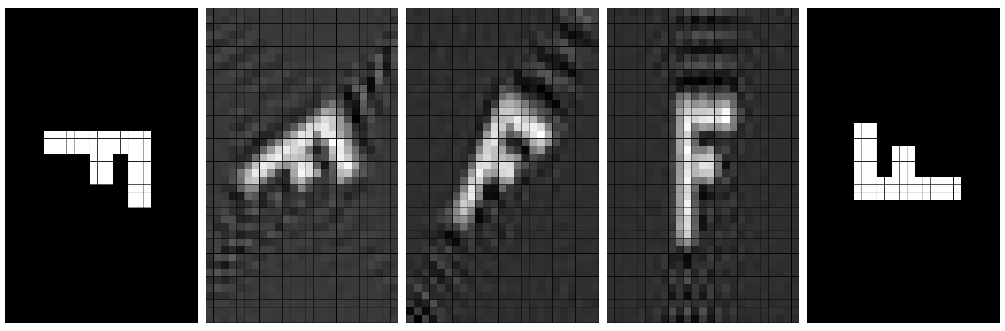
Figure 3: On a $41\times 25$ pixellated screen, $(j_{x},j_{y})=(20,12)$, successive rotations by $\frac{1}{6}\pi$ of the top image, to $\frac{1}{6}$, $\frac{1}{3}\pi$, $\frac{1}{2}\pi$, and (extreme right) $\pi$, of a white image on black background. The gray-level scale is adjusted to the smallest and largest values of the set of pixels; for the $\pi=\frac{1}{3}$ image, these are $(-0.31374,1.38345)$.

4.2 Symmetric and antisymmetric Fourier transforms

In the continuous model, the mode number operators $\bar{H}_{x}$ and $\bar{H}_{y}$ generate fractional Fourier transforms [9] through $\bar{\cal F}_{k}(\beta_{k})=\exp(-{\rm i}\beta_{k}\bar{H}_{k})$ that multiply the continuous oscillator basis functions $\Psi_{n_{x}}^{\scriptscriptstyle\rm HG}(q_{k})$ by phases $\exp(-{\rm i}n_{k}\beta_{k})$. In the finite oscillator model, the symmetric fractional Fourier-Kravchuk transform ${\cal K}_{\scriptscriptstyle\rm S}(\chi):=\exp(-2{\rm i}\chi L_{0})$ is generated by $L_{0}={\textstyle\frac{1}{2}}(K_{x}{+}K_{y})$ as in (5). It acts on the Cartesian modes only multiplying them by phases,

$$\begin{array}[]{l}{\cal K}_{\scriptscriptstyle\rm S}(\chi):\Psi_{n_{x},n_{y}}^{(j_{x},j_{y})}(q_{x},q_{y})\\ {\qquad}=\exp[{-{\rm i}\chi(n_{x}+n_{y})}]\,\Psi_{n_{x},n_{y}}^{(j_{x},j_{y})}(q_{x},q_{y}),\end{array}$$ (18)

and commutes with all transformations in the Fourier group.

On the other hand, a rotation by $2\beta$ around the 1-axis is generated by $L_{1}={\textstyle\frac{1}{2}}(K_{x}{-}K_{y})$ in (6) to produce the antisymmetric fractional Fourier-Kravchuk transforms, ${\cal K}_{\scriptscriptstyle\rm A}(\beta):=\exp(-2{\rm i}\beta L_{1})$ in the group $\hbox{\sf SU($2$)}_{x}\oplus\hbox{\sf SU($2$)}_{y}$:

$$\begin{array}[]{l}{\cal K}_{\scriptscriptstyle\rm A}(\beta):\Psi_{n_{x},n_{y}}^{(j_{x},j_{y})}(q_{x},q_{y})\\ {\qquad}=\exp[{-{\rm i}\beta(n_{x}-n_{y})}]\,\Psi_{n_{x},n_{y}}^{(j_{x},j_{y})}(q_{x},q_{y}).\end{array}$$ (19)

As with rotations, they can be applied to arbitrary images using the decomposition in (14) on the pixellated screen. Both ${\cal K}_{\scriptscriptstyle\rm S}(\chi)$ and ${\cal K}_{\scriptscriptstyle\rm A}(\beta)$ are ‘domestic’ within ${\hbox{\sf SU($2$)}}_{x}\oplus{\hbox{\sf SU($2$)}}_{y}$ but they mesh apropriately with the imported rotations.

4.3 Gyrations

In the continuous model, gyrations by $\gamma$ around the 2-axis are generated by $\bar{L}_{2}$ in (7). For $\gamma=\frac{1}{4}\pi$ they transform Hermite-Gauss to Laguerre-Gauss modes and can be realized with simple paraxial optical setups [16, 17, 18]. They are rotations that result from a rotation by ${\textstyle\frac{1}{2}}\pi$ around the 3-axis (antisymmetric fractional Fourier transform by angle $\frac{1}{4}\pi$), a rotation $\gamma$ around the new 1-axis, and back through $-{\textstyle\frac{1}{2}}\pi$ around the new $3$-axis,

$$\bar{\cal G}(\gamma):=\bar{\cal F}_{\scriptscriptstyle\rm\!\!A}({\textstyle\frac{1}{4}}\pi)\,\bar{\cal R}(\gamma)\,\bar{\cal F}_{\scriptscriptstyle\rm\!\!A}(-{\textstyle\frac{1}{4}}\pi).$$ (20)

We can thus import gyrations into the finite model through replacing $\bar{\cal F}_{\scriptscriptstyle\rm\!\!A}\mapsto{\cal K}_{\scriptscriptstyle\rm A}$ in (19) and (20) [6]. On the Cartesian Kravchuk modes $\Psi_{n_{x},n_{y}}^{(j_{x},j_{y})}(q_{x},q_{y})$, gyration will thus act as

$$\begin{array}[]{l}{\cal G}(\gamma):\Psi_{n_{x},n_{y}}^{(j_{x},j_{y})}(q_{x},q_{y})\\[3.0pt] \displaystyle{\qquad}:=e^{-{\rm i}\pi(n_{x}-n_{y})/4}\!\!\!\!\!\sum_{n^{\prime}_{x}+n^{\prime}_{y}=n}\!\!\!d^{\lambda(n)}_{\mu,\mu^{\prime}}(2\gamma)\\ {\qquad\qquad\qquad}\times e^{+{\rm i}\pi(n^{\prime}_{x}-n^{\prime}_{y})/4}\,\Psi_{n^{\prime}_{x},n^{\prime}_{y}}^{(j_{x},j_{y})}(q_{x},q_{y}).\end{array}$$ (21)

where $\lambda(n)$, $\mu$ and $\mu^{\prime}$ are related to $j_{x},\,n_{x},\,j_{y},\,n_{y}$ through (16). This set of functions forms also, as in the Cartesian case, a complete and orthogonal basis for all images on the pixellated screen. We show the gyration of modes $\Psi_{n_{x},n_{y}}^{(j_{x},j_{y})}(q_{x},q_{y})$ in Fig. 4 for various values of $0\leq\gamma\leq\frac{1}{4}\pi$. Note that this transformation yields complex arrays of functions, so for $\gamma=\frac{1}{4}\pi$ we show their absolute values and phases.

For $\gamma=\frac{1}{4}\pi$, (21) defines finite functions characterized by the total mode number $n:=n_{x}{+}n_{y}$ and an integer ‘(rectangular) angular momentum’ number $m=2\mu=n_{x}{-}n_{y}$, $|\mu|\leq\lambda(n)$ constrained by (16), and given by

$$\begin{array}[]{l}\displaystyle\Lambda_{n,m}^{\!(j_{x},j_{y})}(q_{x},q_{y}):=e^{-{\rm i}\pi(n_{x}-n_{y})/4}\!\!\!\!\!\!\sum_{n^{\prime}_{x}+n^{\prime}_{y}=n}\!\!\!d^{\lambda(n)}_{\mu,\mu^{\prime}}({\textstyle\frac{1}{2}}\pi)\\ {\qquad\qquad\quad\qquad}\times e^{+{\rm i}\pi(n^{\prime}_{x}-n^{\prime}_{y})/4}\,\Psi_{n^{\prime}_{x},n^{\prime}_{y}}^{(j_{x},j_{y})}(q_{x},q_{y})\\ {\qquad\qquad\quad\qquad}=\Lambda_{n,-m}^{\!(j_{x},j_{y})}(q_{x},q_{y})^{*}.\end{array}$$ (22)

In the square screen case, when $j_{x}=j=j_{y}$, the functions $\Lambda_{n,m}^{(j)}(q_{x},q_{y})$ were called Laguerre-Kravchuk modes [6], whose continuous counterparts are the well-known Laguerre-Gauss modes. Within rectangular pixellated screens, the functions (22) are also orthogonal and complete,

$${}\!\!\!\!\!\!\sum_{n,m}\Lambda_{n,m}^{\!(j_{x},j_{y})}(q_{x},q_{y})^{*}\,\Lambda_{n,m}^{(j_{x},j_{y})}(q^{\prime}_{x},q^{\prime}_{y}) = \delta_{q_{x},q^{\prime}_{x}}\delta_{q_{y},q^{\prime}_{y}},$$ (23)

$${}\!\!\!\!\!\!\sum_{q_{x},q_{y}}\Lambda_{n,m}^{\!(j_{x},j_{y})}(q_{x},q_{y})^{*}\,\Psi_{n^{\prime},m^{\prime}}^{(j_{x},j_{y})}(q_{x},q_{y}) = \delta_{n,n^{\prime}}\delta_{m,m^{\prime}},$$ (24)

since they are obtained from the Cartesian states through $\hbox{\sf su($2$)}_{\scriptscriptstyle\rm F}$ unitary transformations. Although the notion of their angular momentum is no longer properly valid, they still bear a recognizable resemblance, as Fig. 5 shows, where the multiplets $\{\Lambda_{n,m}^{\!(j_{x},j_{y})}(q_{x},q_{y})\}_{m=-\lambda(n)}^{\lambda(n)}$ are placed on rows for all total modes $n$ in the three intervals (16).

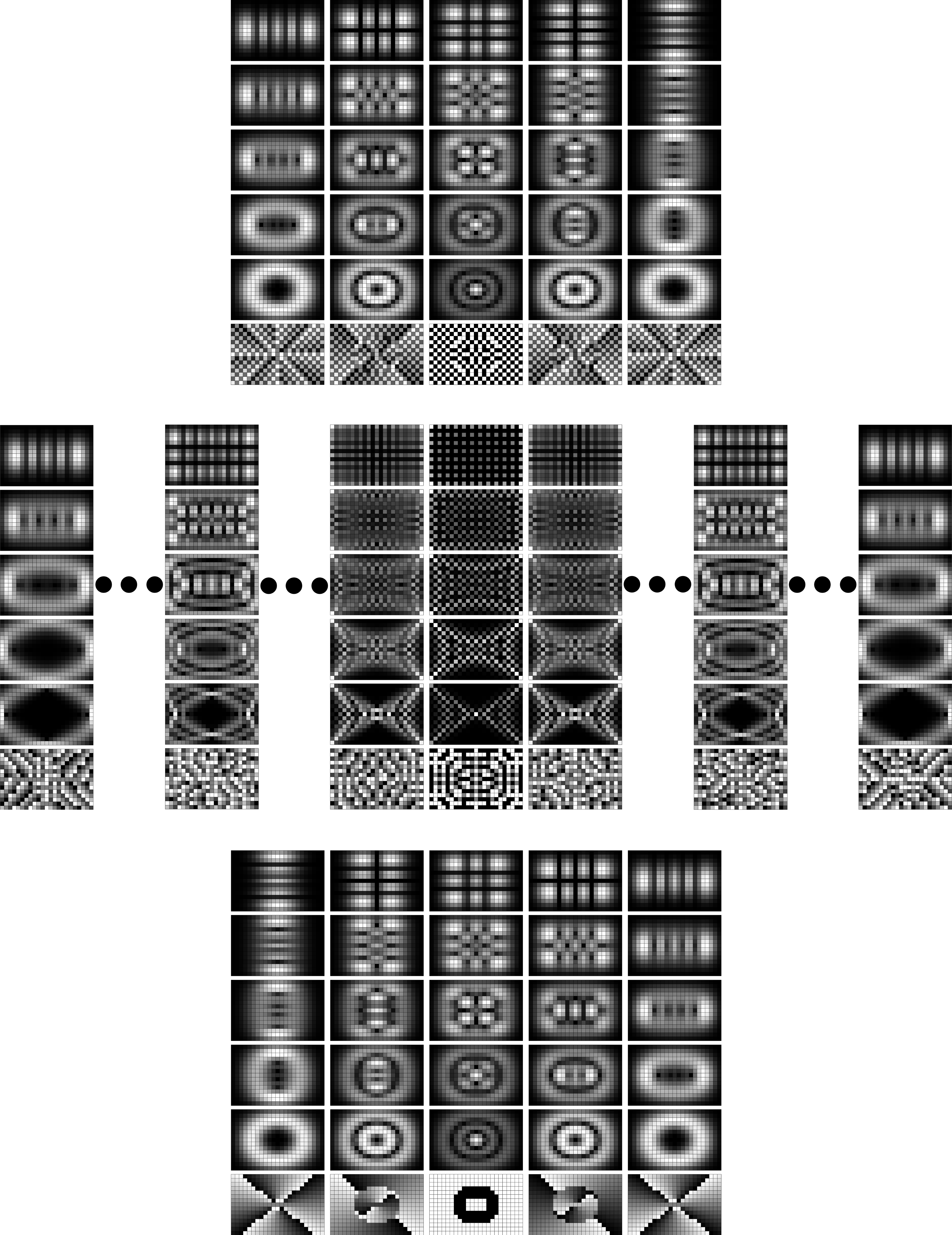
Figure 4: Gyrations of selected Cartesian Kravchuk modes $\Psi_{n_{x},n_{y}}^{(11,7)}(q_{x},q_{y})$ in (21) by $\gamma=0$, $\frac{1}{16}\pi$ , and $\frac{1}{8}\pi$, $\frac{3}{16}\pi$, and $\frac{1}{4}\pi$. Since the modes are complex, we show their absolute values; the bottom row of each block shows the phase of the $\frac{1}{4}\pi$ gyration. As in Fig. 2, we display multiplets in each of the three blocks according to the three intervals in (16). Bottom: the level $n=4$ ($\lambda=2$) in the lower triangle. Middle: selected states in the mid rhomboid at level $n=18$ ($\lambda=7$). Top: states in the level $n=32$ ($\lambda=2$).

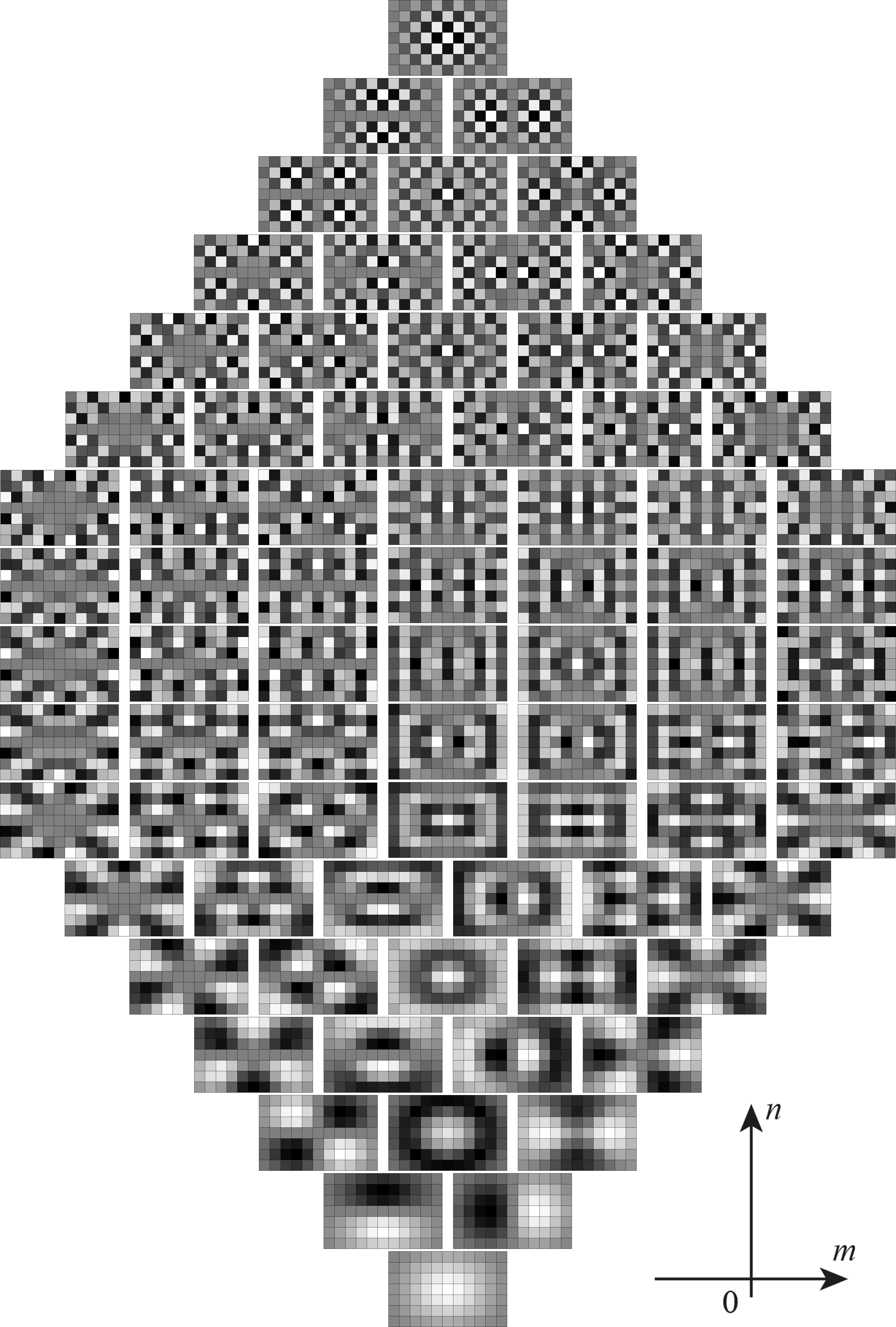
Figure 5: The rectangular ‘Laguerre-Kravchuk’ modes $n$ of ‘angular momentum’$m$, $\Lambda_{n,m}^{\!(j_{x},j_{y})}(q_{x},q_{y})$ in (22). Since the modes are complex, on the right-hand side $m\geq 0$ we show the density plot of the real part, and on the left-hand side $m<0$ the imaginary part of the $m>0$ functions. The $m=0$ modes are real.

5 Concluding remarks

In continuous systems, the elements of the $\hbox{\sf U($2$)}_{\scriptscriptstyle\rm F}$ Fourier group can be parametrized by the angle of the central symmetric Fourier transform and three $\hbox{\sf SU($2$)}_{\scriptscriptstyle\rm F}$ Euler angles as

$$\begin{array}[]{rcl}\bar{\cal D}(\chi;\psi,\theta,\phi)&=&\exp(-{\rm i}\chi\bar{L}_{0})\\ &\times&\exp(-{\rm i}\psi\bar{L}_{3})\exp(-{\rm i}\theta\bar{L}_{2})\exp(-{\rm i}\phi\bar{L}_{3}).\end{array}$$ (25)

On the finite $N_{x}\times N_{y}$ pixellated screen, $\hbox{\sf U($2$)}_{\scriptscriptstyle\rm F}$ is correspondingly realized by subgroups of domestic Fourier-Kravchuk transformations, and imported rotations and gyrations, as

$$\begin{array}[]{l}{\cal D}(\chi;\psi,\theta,\phi)={\cal K}_{\scriptscriptstyle\rm S}({\textstyle\frac{1}{2}}\chi)\,{\cal K}_{\scriptscriptstyle\rm A}({\textstyle\frac{1}{2}}\psi)\,{\cal G}({\textstyle\frac{1}{2}}\theta)\,{\cal K}_{\scriptscriptstyle\rm A}({\textstyle\frac{1}{2}}\phi)\\[3.0pt] {\qquad}={\cal K}_{\scriptscriptstyle\rm S}({\textstyle\frac{1}{2}}\chi)\,{\cal K}_{\scriptscriptstyle\rm A}({\textstyle\frac{1}{2}}\psi{+}{\textstyle\frac{1}{4}}\pi)\,{\cal R}({\textstyle\frac{1}{2}}\theta)\,{\cal K}_{\scriptscriptstyle\rm A}({\textstyle\frac{1}{2}}\phi{-}{\textstyle\frac{1}{4}}\pi).\end{array}$$ (26)

The action of the Fourier group is unitary on all complex-valued images on $N_{x}\times N_{y}$ pixellated screens, and hence there is no information loss under these transformations. We must repeat that the algorithm is not fast, but arguably the slowest, and will necessarily involve Gibbs-like oscillations in pixellated images with sharp ‘discontinuities’. As the previous experience with square screens suggests [5], smoothing the original values or chopping the resulting ones can restore the visual fidelity of the image, even though unitarity will be lost. It may be that in experiments where two-dimensional beams are sampled at rectangular CCD arrays, bases of discrete functions are better suited for the task than their approximation by pointwise-sampled Hemite-Gauss oscillator wavefunctions [19].

The introduction of rectangular analogues of the Laguerre-Gauss states with ‘angular momentum’ is the direct (but not trivial) generalization of those built for square screens in Ref. [4] and, as there, will predictably allow a unitary map to screens whose pixels are arranged along polar coordinates, as done in Ref. [20]. Finally, it should be noted that all the ‘discrete’ functions, starting with the Wigner little-$d^{j}_{n-j,q}(\theta)$, are actually analytic functions of continuous position $q$ in the range $-j{-}1<q<j{+}1$, with branch-point zeros at $q=\pm(j{+}1)$ and cuts beyond. This property extends of course to the two-dimensional case for $-j_{k}{-}1<q_{k}<j_{k}{+}1$, $k\in\{x,y\}$. The discrete model can thus also accommodate a continuous model of modes in bounded screens, although the unitarity of the transformations holds only for the discrete integer points within.

References

- [1] R. Simon and K.B. Wolf, “Fractional Fourier transforms in two dimensions,” J. Opt. Soc. Am. A 17, 2368–2381 (2000).
- [2] S.A. Collins, “Lens-system diffraction integral written in terms of matrix optics,” J. Opt. Soc. Am. 60, 1168–-1177 (1970).
- [3] M. Moshinsky and C. Quesne, “Linear canonical transformations and their unitary representations,” J. Math. Phys. 12, 1772–-1780 (1971).
- [4] N.M. Atakishiyev, G.S. Pogosyan, L.E. Vicent, and K.B. Wolf, “Finite two-dimensional oscillator: I. The Cartesian model,” J. Phys. A: Math. Gen. 34, 9381–9398 (2001).
- [5] L.E. Vicent, “Unitary rotation of square-pixellated images,” Appl. Math. Comput. 221, 111–117 (2009).
- [6] K.B. Wolf and T. Alieva, “Rotation and gyration of finite two-dimensional modes,” J. Opt. Soc. Am. A 25, 365–370 (2008).
- [7] L. Barker, Ç. Çandan, T. Hakioğlu, and H.M. Ozaktas, “The discrete harmonic oscillator, Harper’s equation, and the discrete fractional Fourier transform,” J. Phys. A: Math. Gen. 33, 2209–2222 (2000).
- [8] L. Barker, “Continuum quantum systems as limits of discrete quantum systems: II. State functions,” J. Phys. A: Math. Gen. 34, 4673–4682 (2001).
- [9] N.M. Atakishiyev and K.B. Wolf, “Fractional Fourier-Kravchuk transform,” J. Opt. Soc. Am. A 14, 1467–1477 (1997).
- [10] L. Allen, M.J. Padgett and M. Babiker, “The orbital angular momentum of light” Progress in Optics, ed. E. Wolf, Vol. XXXIX (Elsevier, 1999), pp. 294–374.
- [11] N.M. Atakishiyev, G.S. Pogosyan, and K.B. Wolf, “Contraction of the finite one-dimensional oscillator,” Int. J. Mod. Phys. A 18, 317–327 (2003).
- [12] L.C. Biedenharn and J.D. Louck, “Angular Momentum in Quantum Mechanics,” Encyclopedia of Mathematics and its Applications G.-C. Rota, ed. (Addison-Wesley, 1981); Sect. 3.6.
- [13] N.M. Atakishiyev and S.K. Suslov, “Difference analogs of the harmonic oscillator,”Theor. Math. Phys. 85, 1055–1062 (1991).
- [14] M. Krawtchouk, “Sur une généralization des polinômes d’Hermite,” C. R. Acad. Sci. Paris 189, 620–622 (1929).
- [15] N.M. Atakishiyev, G.S. Pogosyan, and K.B. Wolf, “Finite models of the oscillator,” Phys. Part. Nucl. 36, Suppl. 3, 521–555 (2005).
- [16] M.J. Bastiaans and T. Alieva, “First-order optical systems with unimodular eigenvalues,” J. Opt. Soc. Am. A 23, 1875–1883 (2006).
- [17] T. Alieva and M.J. Bastiaans, “Orthonormal mode sets for the two-dimensional fractional Fourier transform,” Opt. Lett. 32, 1226–1228 (2007).
- [18] J.A. Rodrigo, T. Alieva and M.L. Calvo, “Gyrator transform: properties and applications,” Opt. Express 15, 2190–2203 (2007).
- [19] L.E. Vicent and K.B. Wolf, “Analysis of digital images into energy-angular momemtum modes,” J. Opt. Soc. Am. A 28, 808–814 (2011).
- [20] N.M. Atakishiyev, G.S. Pogosyan, L.E. Vicent and K.BẆolf, “Finite two-dimensional oscillator. II: The radial model,” J. Phys. A: Math. Gen. 34, 9399–9415 (2001).