Scalar doublet models confront $\tau$ and $b$ anomalies

Abstract

There are indications of a possible breakdown of the standard model, suggesting that $\tau$ lepton interactions violate flavor universality, particularly through $B$ meson decays. BABAR, Belle and LHCb report high ratios of $B\to D^{(*)}\tau\nu$. There are long-standing excesses in $B\to\tau\nu$ and $W\to\tau\nu$ decays, and a deficit in inclusive $\tau$ to strange decays. We investigate whether two Higgs doublet models with the most general allowed couplings to quarks, and a large coupling to $\tau$ leptons, can explain these anomalies while respecting other flavor constraints and technical naturalness. Fits to $B\to D^{(*)}\tau\nu$ data require couplings of the new Higgs doublet to down-type quarks, opening the door to many highly constrained flavor-changing neutral current (FCNC) processes. We confront these challenges by introducing a novel ansatz that relates the new up- and down-type Yukawa couplings, and demonstrate viable values of the couplings that are free from fine tuning. LEP and LHC searches for new Higgs bosons decaying via $H^{0}\to\tau^{+}\tau^{-}$ and $H^{\pm}\to\tau^{\pm}\nu$ allow a window of masses $m_{H}=[100$-$125]\,$GeV and $m_{\pm}\sim 100\,$GeV that is consistent with the predictions of our model. Contamination of the $W^{+}\to\tau^{+}\nu$ signal by $H^{+}\to\tau^{+}\nu$ decays at LEP could explain the apparent $W\to\tau\nu$ excess. We predict that the branching ratio for $B_{s}\to\tau^{+}\tau^{-}$ is not far below its current limit of several percent. An alternative model with decays of $B\to D^{(*)}\tau\nu_{s}$ to a sterile neutrino is also argued to be viable.

I Introduction

The origin of the Standard Model (SM) flavor structure is a mystery, and any model predicting new patterns of flavor violation must confront very strong experimental bounds. This has given rise to the Minimal Flavor Violation (MFV) paradigm Chivukula:1987py ; D'Ambrosio:2002ex ; Cirigliano:2005ck ; Kagan:2009bn as a guide for constructing new physics beyond the SM, that has been highly influential in recent years. MFV is extremely effective for suppressing flavor changing neutral currents (FCNCs). In this work we confront some hints of new physics for which MFV seems generally too strong to accommodate the observed deviations. We are thus motivated to consider an alternative that can allow for larger nonstandard flavor effects.

Several recent experiments indicate possible deviations from the SM in some flavor-specific observables involving $\tau$ leptons. BaBar, Belle, and LHCb report the ratios $R(D)$ and $R(D^{*})$, defined as

$$R(X)=\frac{\mathcal{B}(\bar{B}\rightarrow X\,\tau\,\bar{\nu})}{\mathcal{B}(\bar{B}\rightarrow X\,\ell\,\bar{\nu})}$$ (1)

where $\ell=e,\mu$. The summary of the SM predictions and the measurements is shown in table 1. The reported measurements are consistent with each other, and with previously reported results Lees:2012xj ; Huschle:2015rga ; Aaij:2015yra . The measurements are also consistent with $e/\mu$ universality. However, the naively combined experimental value for the ratio $R(D^{(\star)})$ differs from the SM prediction by more than $3\,\sigma$.

-	$R(D)$	$R(D^{*})$
SM	0.297 $\pm$ 0.017	0.252 $\pm$ 0.005
Belle Huschle:2015rga	0.375 ${\scriptstyle\pm 0.064\pm 0.026}$	0.293 ${\scriptstyle\pm 0.038\pm 0.015}$
BaBar Lees:2012xj	0.440 ${\scriptstyle\pm 0.058\pm 0.042}$	0.332 ${\scriptstyle\pm 0.024\pm 0.018}$
LHCb Aaij:2015yra		0.336 ${\scriptstyle\pm 0.027\pm 0.030}$
Expt.  avg.:	0.408 $\pm$ 0.050	0.321 $\pm$ 0.021

Table 1: Summary of experimental and predicted values for $R(D)$ and $R(D^{*})$.

There have been other hints of a breakdown of lepton flavor universality between $\tau$ and $e/\mu$. The measured decay rate of $B\to\tau\nu$ displays some tension with the SM prediction. Although a recent measurement by Belle Adachi:2012mm has reduced the discrepancy to the level of $1.7\,\sigma$, the current world average measurement remains a factor of 1.5 higher than the SM prediction (see ref. Soffer:2014kxa for a recent review.) The observed rate of $W\to\tau\nu$ is also in tension with the standard model predictions: the LEP measurement is $\sim 10\%$ above the SM value, at $2.4\,\sigma$ significance. The inclusive decays of $\tau$ to strange quarks yield a value of the CKM matrix element $V_{us}$ significantly lower than that required for unitarity Lusiani:2015eja .

A number of authors have studied $B\to D^{(*)}\tau\nu$ in the context of type-III two Higgs doublet models (2HDMs), in which the most general couplings of fermions to both doublets are allowed, as well as model-independent analyses that include this framework Fajfer:2012jt ; Datta:2012qk ; Crivellin:2012ye ; Celis:2012dk ; Tanaka:2012nw ; Freytsis:2015qca ; Crivellin:2015hha . There are two possible operators contributing to the hadronic part of these processes, mediated by charged Higgs exchange, proportional to $C^{cb}_{S_{R}}\bar{c}_{L}\,b_{R}$ and $C^{cb}_{S_{L}}\bar{c}_{R}\,b_{L}$, respectively. (For simplicity we assume that the coefficients are real in the present work.) Some studies Fajfer:2012jt ; Crivellin:2012ye ; Celis:2012dk ; Tanaka:2012nw ; Crivellin:2015hha found that $C^{cb}_{S_{L}}$ by itself is sufficient to get a good fit to the observed decay rates. However several recent analyses Lees:2013uzd ; Freytsis:2015qca obtain best-fit regions requiring $C^{cb}_{S_{R}}\sim-C^{cb}_{S_{L}}$. In particular, these studies use not only the total rates but also the differential decay distributions as inputs to their fits, finding that $C^{cb}_{S_{L}}$ by itself does not fit the decay spectra.

This difference is crucial for model building, since having $C^{cb}_{S_{L}}\neq 0$ only requires that the new up-type Yukawa matrix $\rho_{u}$ (which couples mainly to the nonstandard Higgs doublet) is important, while keeping the down-type couplings $\rho_{d}\cong 0$. If $C^{cb}_{S_{R}}$ is also large, then $\rho_{d}\sim\rho_{u}$, making it much more challenging to satisfy constraints on FCNCs. The purpose of this paper is to see how far one can go toward overcoming these challenges, within the context of 2HDMs, if the indication for $C^{cb}_{S_{R}}\sim-C^{cb}_{S_{L}}$ persists in future analyses.

We will show that some of the flavor challenges can be addressed if $\rho_{u}$ and $\rho_{d}$ are related to each other in a particular way that involves the CKM matrix. This is a new ansatz for helping to give flavor protection to type III 2HDMs, which might be of interest more generally than for the particular applications that motivated us here. It is quite different from MFV, yet it appears to facilitate adequate control over FCNCs to make the theory viable, especially in the down-quark sector where the constraints are strongest.

The model is strongly constrained by LEP and LHC searches for the new charged Higgs decaying into $\tau\nu$ and the neutral one decaying to $\tau^{+}\tau^{-}$. We find a window $\sim[100$-$125]\,$GeV of allowed masses for the new scalars that passes the collider constraints while allowing for an explanation of the $B$ decay anomalies. Scalars of these masses are just beyond the kinematic reach of LEP, while being in a region of low efficiency for LHC searches, if their couplings to quarks are sufficiently small.

The outline of the paper is as follows. In section II we define the model. In section III we derive constraints on the new Yukawa couplings $\rho_{\nu}$, $\rho_{u}$, $\rho_{d}$ arising from fits to $R(D)$ and $B\to\tau\nu$, and a few key flavor-sensitive decays. Section IV examines the collider constraints determining the allowed mass range of the new $\sim 100\,$GeV Higgs bosons. In section V we present a novel ansatz relating $\rho_{u}$ and $\rho_{d}$, that allows these constraints to be satisfied in a controlled way. It is a linear relation involving the CKM matrix $V$, a diagonal unitary matrix $U$, and an $O(1)$ parameter $\eta$: $\rho_{u}^{\dagger}V=\eta\,UV\rho_{d}$.

In section VI we calculate observables from meson oscillations that most strongly constrain the scenario, while in section VII we show that rare decay processes that might challenge it are within the experimental limits. Section VIII obtains a numerical fit to the couplings $\rho_{d}^{ij}$, that determine $\rho_{u}$ through our ansatz. In section IX we estimate the size of loop contributions to the nonstandard Yukawa and Higgs couplings to establish technical naturalness of the model. In section X we outline a microscopic model that naturally implements the “charge transformation” mechanism for relating $\rho_{u}$ and $\rho_{d}$ in the manner of our ansatz. We outline an alternative version of the model in section XI, where the leptonic coupling $\rho_{e}$ is replaced by a coupling $\rho_{\nu}$ to neutrinos, assuming a light sterile neutrino in the anomalous decays of $B$, rather than $\nu_{\tau}$. This model is less constrained by LHC searches for the neutral Higgs. Conclusions are given in section XII. Details of the sterile neutrino version of the model are given in the appendix.

II The model

We begin with the most general two Higgs doublet model, where $H_{1}$ and $H_{2}$ are the doublets, each coupling to all the fermions. They have the conventional decomposition

$$H_{1}=\frac{1}{\sqrt{2}}\,\left(\begin{array}[]{c}{\sqrt{2}\,H_{1}^{+}}\\ {v+H_{1}^{r}+iH_{1}^{i}}\end{array}\right),\quad H_{2}=\frac{1}{\sqrt{2}}\,\left(\begin{array}[]{c}{\sqrt{2}\,H_{2}^{+}}\\ {H_{2}^{r}+iH_{2}^{i}}\end{array}\right)$$ (6)

in terms of the real and imaginary parts of the neutral components. The Yukawa coupling Lagrangian is

$${\cal L}_{Y} = -{\bar{Q}}_{L}\,\hat{y}_{u}\,\tilde{H}_{1}\,{u}_{R}-{\bar{Q}}_{L}\,\hat{y}_{d}\,H_{1}\,{d}_{R}-{\bar{L}}_{L}\,\hat{y}_{e}\,H_{1}\,{e}_{R},$$

$$-{\bar{Q}}_{L}\,\hat{\rho}_{u}\,\tilde{H}_{2}\,{u}_{R}-{\bar{Q}}_{L}\,\hat{\rho}_{d}\,H_{2}\,{d}_{R}-{\bar{L}}_{L}\,\hat{\rho}_{e}\,H_{2}\,{e}_{R}+{\rm h.c.}$$

where flavor, color and ${\rm SU(2)}_{L}$ indices have been suppressed, and $\tilde{H}_{i}^{a}=\epsilon_{ab}H_{i}^{b\star}$. The scalar Lagrangian is given by

$${\cal L}_{S} = |D^{\mu}H_{1}|^{2}+|D^{\mu}H_{2}|^{2}-V(H_{1},H_{2})$$ (8)

where the potential is defined as

$$V = \lambda\,\left(H_{1}^{\dagger}\,H_{1}-\frac{v^{2}}{2}\right)^{2}+m_{2}^{2}\,(H_{2}^{\dagger}\,H_{2}),$$

$$+ (m_{12}^{2}\,(H_{1}^{\dagger}H_{2})+{\rm h.c.})+\lambda_{1}\,(H_{1}^{\dagger}H_{1})\,(H_{2}^{\dagger}H_{2})$$

$$+ \lambda_{2}\,(H_{1}^{\dagger}H_{2})\,(H_{2}^{\dagger}H_{1})+\left[\lambda_{3}(H_{1}^{\dagger}H_{2})^{2}+{\rm h.c.}\right]$$

$$+ \left[\lambda_{4}(H_{1}^{\dagger}H_{2})(H_{2}^{\dagger}H_{2})+\lambda_{5}(H_{2}^{\dagger}H_{1})(H_{1}^{\dagger}H_{1})+{\rm h.c.}\right]$$

$$+ \lambda_{6}(H_{2}^{\dagger}H_{2})^{2}.$$

In this basis of fields, $H_{2}$ has no vacuum expectation value, requiring the condition $m_{12}^{2}+\lambda_{5}^{\star}v^{2}/2=0$. This is just a choice of field coordinates, which in general can always be achieved by doing a rotation (conventionally denoted by angle $\beta$ as well as a possible rephasing) between $H_{1}$ and $H_{2}$; however in section X we will argue that the Yukawa couplings were generated directly in this basis, so that the $\hat{y}$ and $\hat{\rho}$ matrices can naturally have very different magnitudes and structures.

For simplicity we will assume that the potential (II) is CP-conserving, so that there is no mixing between scalars and the pseudoscalar. The rotation between the Higgs basis fields and the CP-even mass eigenstates is

$$\left(\begin{array}[]{c}{H_{2}^{r}}\\ {H_{1}^{r}}\end{array}\right)=\left(\begin{array}[]{cc}c_{\scriptscriptstyle\beta\alpha}&-s_{\scriptscriptstyle\beta\alpha}\\ s_{\scriptscriptstyle\beta\alpha}&\phantom{-}c_{\scriptscriptstyle\beta\alpha}\end{array}\right)\,\left(\begin{array}[]{c}{h}\\ {H}\end{array}\right)$$ (16)

Here we have used notation that is conventional in 2HDMs, such that for $s_{\scriptscriptstyle\beta\alpha}\cong 1$, the SM-like Higgs boson $h$ is mostly $H_{1}^{r}$. For small $|c_{\scriptscriptstyle\beta\alpha}|$, the mixing angle is approximately determined by

$$c_{\scriptscriptstyle\beta\alpha}\cong{\lambda_{5}\,v^{2}\over 2(m_{h}^{2}-m_{H}^{2})}$$ (17)

where the SM-like, new neutral and charged Higgs boson masses are respectively

$$m_{h}^{2} \cong 2\lambda v^{2}$$

$$m_{H}^{2} \cong m_{2}^{2}+{\textstyle{1\over 2}}(\lambda_{1}+\lambda_{2}+2\lambda_{3})\,v^{2}$$

$$m_{A}^{2} \cong m_{H}^{2}-2\lambda_{3}v^{2}$$

$$m_{\pm}^{2} = m_{2}^{2}+{\textstyle{1\over 2}}\lambda_{1}v^{2}$$ (18)

These approximations are valid for small mixing. We will also require that the splittings between masses of the neutral scalars $H$, $A$ (CP-even and CP-odd respectively) are small, so that they can be regarded as components of a complex neutral field for most purposes. This not only simplifies the model but also proves useful for suppressing some FCNC effects as we will show. Small splittings are consistent with $|c_{\scriptscriptstyle\beta\alpha}|\ll 1$ and $|\lambda_{3}|\ll 1$, since it can be shown (without any approximation) that

$$m^{2}_{H}-m^{2}_{A} = c_{\scriptscriptstyle\beta\alpha}^{2}(m_{H}^{2}-m_{h}^{2})+2\lambda_{3}v^{2}$$ (19)

(see for example Sierra:2014nqa ). We will therefore assume that $|\lambda_{3}|\ll 1$ in addition to $|c_{\scriptscriptstyle\beta\alpha}|\ll 1$. Although $\lambda_{2}$ could a priori be relatively large, in this work we will be interested in masses of order $m_{H}\lesssim m_{h}$ and $m_{\pm}\sim 100\,$GeV, corresponding to $\lambda_{2}\lesssim 0.2$. Electroweak precision data (see eq. (10.26) of ref. PDG ) would allow for larger splittings, with $m_{H}$ as large as $175\,$GeV for $m_{\pm}\sim 100\,$GeV. The couplings $\lambda_{4},\,\lambda_{6}$ play no direct role for our predictions, but can be relevant for understanding the expected size of radiative corrections to the $\lambda_{i}$ couplings, as we will discuss in section IX. Vacuum stability requires that $\sqrt{\lambda\lambda_{6}/2}>-\lambda_{2}$ if $\lambda_{2}<0$.

As usual, biunitary rotations on the quark fields in ${\cal L}_{Y}$ diagonalize $\hat{y}_{u}$, $\hat{y}_{d}$, $\hat{y}_{e}$, with the scalar doublets still in the Higgs basis. The subsequent rotation (16) then brings ${\cal L}_{Y}$ to the form

$${\cal L}_{Y} = -{1\over\sqrt{2}}\sum_{\phi=h,H,A\atop f=u,d,e}y^{f}_{\phi ij}\,\bar{f}_{i}\phi P_{\scriptscriptstyle R}f_{j}+{\rm h.c.}$$ (20)

$$y^{f}_{hij} = s_{\scriptscriptstyle\beta\alpha}{\sqrt{2}\,m_{f}^{i}\over v}\delta_{ij}+c_{\scriptscriptstyle\beta\alpha}\rho_{f}^{ij},$$ (21)

$$y^{f}_{Hij} = c_{\scriptscriptstyle\beta\alpha}{\sqrt{2}\,m_{f}^{i}\over v}\delta_{ij}-s_{\scriptscriptstyle\beta\alpha}\rho_{f}^{ij},$$ (22)

$$y^{f}_{Aij} = \rho_{f}^{ij}\times\left\{{\textstyle{\!\!\!+i,\ f=u\atop-i,\ f=d,e}}\right.$$

where $P_{\scriptscriptstyle R}=(1+\gamma_{5})/2$ is the usual chiral projector and $v\simeq 246\,$GeV (see for example the discussion in Omura:2015nja ). The matrices $\rho_{f}^{ij}$ with $f=e,u,d$ are in general complex and can induce tree-level FCNCs. They are given explicitly by

$$\rho_{u} = L_{u}^{\dagger}\,\hat{\rho}_{u}\,R_{u},$$

$$\rho_{d} = L_{d}^{\dagger}\,\hat{\rho}_{d}\,R_{d},$$

$$\rho_{e} = L_{e}^{\dagger}\,\hat{\rho}_{e}\,R_{e},$$

where the unitary matrices transform between the weak and mass eigenstates, and determine the CKM matrix $V=L_{u}^{\dagger}L_{d}$. The charged scalars couple to the fermions as

$${\cal L} = -\bar{\nu}\left(U_{\nu}^{\dagger}\,\rho_{e}\right)H^{+}\,P_{\scriptscriptstyle R}\,e$$

$$-\bar{u}\left(V\rho_{d}P_{\scriptscriptstyle R}-\rho_{u}^{\dagger}VP_{\scriptscriptstyle L}\right)H^{+}d+{\rm h.c.}$$

where $U_{\nu}=L_{\nu}^{\dagger}\,L_{e}$ is the PMNS neutrino mixing matrix. Since neutrino oscillations are unimportant in the processes under consideration, we henceforth replace $U_{\nu}\,\nu\to\nu$ with the understanding that $\nu$ refers to the initially emitted flavor eigenstate.

III Explaining the anomalies

Our primary motivation is to present a framework that is able to simultaneously explain the excess signals in processes with final state $\tau$ leptons: $B\to D^{(*)}\tau\nu$, $B\to\tau\nu$ and $W\to\tau\nu$. In addition we consider the hint of a deficit in $\tau\to K^{-}\nu$ decays. In this section we will show how these can come about at tree level due to exchange (or decay) of the charged Higgs $H^{\pm}$, for appropriate choices of the new Yukawa couplings in $\rho_{e}$, $\rho_{d}$ and $\rho_{u}$. The decays of $B$, $B_{s}$ and $h$ into $\tau^{+}\tau^{-}$ provide immediate constraints on the scenario, which we therefore also consider in this section.

III.1 $B\to D\tau\nu$, $B\to D^{(\star)}\tau\nu$

New contributions to $B\to D\tau\nu$ can be mediated by the tree-level exchange of the charged Higgs $H^{\pm}$ if $\rho_{e}^{i\tau}$ is nonzero, as can be seen from eq. (II). The matrix element $\rho_{e}^{\tau\tau}$ turns out to be the optimal choice for satisfying the combined constraints from LHC searches for the neutral boson $H^{0}$ and rare leptonic decays of $B$ and $B_{s}$ mesons. We will therefore assume that $\rho_{e}^{\tau\tau}\neq 0$, while the remaining entries in $\rho_{e}^{ij}$ are very small or vanishing.

Integrating out the $H^{\pm}$ then produces the effective Hamiltonian

$$\mathcal{H} = {\rho_{e}^{\tau\tau*}\over m_{\pm}^{2}}\,\left[\bar{\tau}P_{\scriptscriptstyle L}\nu_{\tau}\right]\left[\bar{c}\left(V\rho_{d}P_{\scriptscriptstyle R}-\rho_{u}^{\dagger}VP_{\scriptscriptstyle L}\right)^{cb}b\right]$$ (25)

$$\equiv {1\over\Lambda^{2}}(\bar{\tau}P_{\scriptscriptstyle L}\nu_{\tau})\left[\,C^{cb}_{S_{R}}(\bar{c}P_{\scriptscriptstyle R}b)+C^{cb}_{S_{L}}(\bar{c}P_{\scriptscriptstyle L}b)\,\right]$$

that is relevant for $b\to c\tau\nu$ at the quark level. Ref. Freytsis:2015qca performed a fit to the $B\to D^{(*)}\tau\nu$ rates and decay spectral using the two operators in (25), which interfere with the standard model contributions. Two viable solutions for the Wilson coefficients were found there, of which the smaller ones correspond to

$${C^{cb}_{S_{R}}\over\Lambda^{2}} \cong {(\rho_{e}^{\tau\tau})^{*}(V\rho_{d})^{cb}\over m_{\pm}^{2}}\ \ \,\cong\ \ {1.25\over{\rm TeV}^{2}}$$ (26)

$${C^{cb}_{S_{L}}\over\Lambda^{2}} \cong -{(\rho_{e}^{\tau\tau})^{*}(\rho_{u}^{\dagger}V)^{cb}\over m_{\pm}^{2}}\cong-{1.02\over{\rm TeV}^{2}}$$ (27)

There is an intriguing relationship between the couplings,

$$(V\rho_{d})^{cb}\cong(\rho_{u}^{\dagger}V)^{cb}$$ (28)

about which we will say more below.

III.2 $B\to\tau\nu$

The contribution of the new charged Higgs to $B^{+}\to\tau^{+}\nu$ decay modifies the branching ratio (BR) as Hou:1992sy ; Fajfer:2012vx ; Crivellin:2012ye

$$\mathcal{B}(B^{+}\rightarrow\tau^{+}\nu) = \frac{G_{F}^{2}|V_{ub}|^{2}}{8\,\pi}m_{\tau}\,\tau_{B}\,f_{B}\,m_{B}\,\left(1-\frac{m_{\tau}^{2}}{m_{B}^{2}}\right)^{2}\,$$ (29)

$$\times \left|1+\frac{m_{B}^{2}}{\bar{m}_{b}\,m_{\tau}}\frac{(C^{ub}_{S_{R}}-C^{ub}_{S_{L}})}{C^{ub}_{SM}}\right|^{2}$$

where $\bar{m}_{b}$ is the $b$-quark $\overline{\rm MS}$ mass, $C^{ub}_{S_{R}}$ and $C^{ub}_{S_{L}}$ are defined analogously to $C^{cb}_{S_{R}}$ and $C^{cb}_{S_{L}}$ in eq. (25) and $C^{ub}_{SM}=4G_{F}\,V_{ub}/\sqrt{2}$.

To estimate the possible allowable size of the new physics (NP) contribution, we take the enhancement factor in the second line of (29) to be less than 2.6, the ratio between the $3\sigma$ maximum allowed value of the world average measurement $(1.14\pm 0.27)\times 10^{-4}$ and the CKMfitter prediction Charles:2015gya $0.76\times 10^{-4}$ of the BR. This gives the bounds

$$-{0.02\over{\rm TeV}^{2}}\lesssim{\rho_{e}^{\tau\tau}\over m_{\pm}^{2}}\left((V\rho_{d})^{ub}+(\rho_{u}^{\dagger}V)^{ub}\right)\lesssim{0.05\over{\rm TeV}^{2}}$$ (30)

Curiously, this suggests a relation similar to (28), but with the opposite sign,

$$(V\rho_{d})^{ub}\cong-(\rho_{u}^{\dagger}V)^{ub}$$ (31)

In section V we will present an ansatz that combines these two conditions in a concise way.

If the indication for a factor of 1.5 excess in the observed versus SM predicted partial width is interpeted as evidence for new physics, then the condition (31) is not a strict equality, and we should replace (30) with the condition

$$\left|{(V\rho_{d})^{ub}+(\rho_{u}^{\dagger}V)^{ub}\over(V\rho_{d})^{cb}+(\rho_{u}^{\dagger}V)^{cb}}\right|\cong 8\times 10^{-3}$$ (32)

where we used (26-27) to eliminate $\rho_{e}^{\tau\tau}/m_{\pm}^{2}$.

III.3 $W\to\tau\nu$

The branching ratios for $W\to\ell\nu$ were measured by the LEP experiments for the individual lepton flavors, from the production of $W^{+}W^{-}$ pairs. The averaged results are PDG

$$B(W\to e\nu) = (10.71\pm 0.16)\%$$

$$B(W\to\mu\nu) = (10.63\pm 0.15)\%$$

$$B(W\to\tau\nu) = (11.38\pm 0.21)\%$$ (33)

The ratio of decays to $\tau\nu$ versus the first two generations is

$$R_{\tau/\ell}={B(W\to\tau\nu)\over{\textstyle{1\over 2}}[B(W\to e\nu)+B(W\to\mu\nu)]}=1.066\pm 0.028$$ (34)

which deviates from 1 by $2.35\,\sigma$. It was suggested by refs. Dermisek:2008dq ; Park:2006gk that the excess could be due to contamination of the $W$ decay signals by charged Higgs bosons with mass close to $m_{W}$ decaying to $\tau\nu$. In a detailed reanalysis of data reported by DELPHI, it was found that the discrepancy could be reduced to 1.03 for a charged Higgs mass of $m_{\pm}=81\,$GeV and $B(H\to\tau\nu)=0.7$, $B(H\to qq)=0.3$, values ruled out by the more recent LEP study Abbiendi:2013hk . Ref. Dermisek:2008dq found that for $B(H\to\tau\nu)=1$, which is the appropriate limit for our model, the observed $R_{\tau/\ell}$ could be explained if $m_{\pm}=94{+4\atop-3}\,$GeV in the $2\sigma$ region. This is marginally compatible with the combined LEP limit of $m_{\pm}<94\,$GeV Abbiendi:2013hk .

More recent LHC measurements of $W\to\tau\nu$ Czyczula:2015mfa do not see evidence for any excess, but this does not contradict having an observable effect at LEP since the production mechanism for $H^{\pm}$ in this case depends upon its coupling to quarks, which is very small in our model. The same remark applies for the Tevatron, where no such effect was observed either.

We do not attempt to reanalyze the LEP signal here, but point out one potentially important difference between our model and those considered previously in this context. We will require a sizable coupling $\rho_{e}^{\tau\tau}\cong 2.5$ leading to a large width for the charged Higgs,

$$\Gamma_{H^{\pm}}={|\rho_{e}^{\tau\tau}|^{2}\over 16\pi}m_{\pm}\cong 12\,{\rm GeV}$$ (35)

for $m_{\pm}=100\,$GeV. This could allow for a greater effect on $R_{\tau/\ell}$ with $m_{\pm}>95\,$GeV than would be possible in the usually assumed case where $H^{\pm}$ width effects are ignored.

III.4 $\tau\to K^{-}\nu$

Decays of $\tau$ into strange particles are among the processes used to determine the CKM matrix element $V_{us}$. The HFAG collaboration recently noted that the inclusive decays of this kind lead to a determination that is $3.4\,\sigma$ below the value consistent with unitarity, while the average from all $\tau$ decays is $2.9\,\sigma$ too low Lusiani:2015eja . This discrepancy could be explained if the contributions from charged Higgs exchange interfere destructively with the SM amplitudes.

Focusing on the specific decay $\tau\to K^{-}\nu$, the new contribution to the amplitude is given by

$${\cal M}_{\tau\to K\nu}=\,{\rho_{e}^{\tau\tau}(V\rho_{d}+\rho_{u}^{\dagger}V)_{us}\,f_{K}\,m_{K}^{2}\over 2\,m_{\pm}^{2}\,(m_{u}+m_{s})}\,(\bar{u}_{\tau}P_{\scriptscriptstyle L}u_{\nu})$$ (36)

Taking the central values of $|V_{us}|=0.2211\pm 0.0020$ determined from $\tau\to K\nu$ and $|V_{us}|=0.2255\pm 0.0010$ from CKM unitarity Lusiani:2015eja , we estimate that

$$(V\rho_{d}+\rho_{u}^{\dagger}V)_{us}\cong-4.2\times 10^{-4}$$ (37)

(assuming fiducial values $\rho_{e}^{\tau\tau}=2.5$ and $m_{\pm}=100\,$GeV that will be preferred below). The minus sign is necessary to get destructive interference between $W^{\pm}$ and $H^{\pm}$ exchange, given that the relative signs of $\rho_{e}^{\tau\tau}$ and $V\rho_{d}$ are fixed by requiring constructive inteference in $B\to D^{*}\tau\nu$ decays.

We will find that there is some mild tension between (37) and other observables (notably $b\to s\gamma$) in the numerical fit to be described in section VIII, so that we do not insist on this potential anomaly in our fits. However it can plausibly fit into the general pattern of deviations in $\tau$ interactions that are addressed by our model.

III.5 Constraint from $h\to\tau^{+}\tau^{-}$

Because of mixing in the scalar sector, the SM-like Higgs acquires small additional couplings $c_{\scriptscriptstyle\beta\alpha}\rho_{f}$ to fermions. They contribute to the partial width of $h$ as

$$\Gamma(h\rightarrow f_{i}\,\bar{f}_{j}+f_{j}\bar{f}_{i}) = N_{c}\,\frac{m_{h}}{16\,\pi}\,\left(|s_{\scriptscriptstyle\beta\alpha}y_{ij}+c_{\scriptscriptstyle\beta\alpha}\rho_{ij}|^{2}\right.$$ (38)

$$\left.\qquad\qquad+\{i\leftrightarrow j\}\right)$$

for all kinematically accessible final states (with $N_{c}$ colors), where $y_{ij}=\sqrt{2}m_{i}\delta_{ij}/v$. In our model, $\rho_{e}^{\tau\tau}$ is the largest new coupling.

New contributions to the decays into $\tau^{+}\tau^{-}$ are constrained by ATLAS and CMS observations Higgs_constraints . Deviations from the SM expectation are characterized by a coupling modifier $\kappa_{\tau}=|1+c_{\scriptscriptstyle\beta\alpha}\rho_{e}^{\tau\tau}/y_{\tau}|\in[0.64,\,1.14]$ at $2\sigma$, where $y_{\tau}$ is the SM Yukawa coupling. We get the least restrictive constraint if $c_{\scriptscriptstyle\beta\alpha}\rho_{e}^{\tau\tau}$ is negative, in which case there are two solutions,

$$|c_{\scriptscriptstyle\beta\alpha}\,\rho_{e}^{\tau\tau}| < 3.7\times 10^{-3}$$

$$-0.022\ <\ c_{\scriptscriptstyle\beta\alpha}\,\rho_{e}^{\tau\tau} < -0.017$$ (39)

at 95% confidence level. Later we will adopt a fiducial value of $\rho_{e}^{\tau\tau}=2.5$. In that case the central value of (39) implies $c_{\scriptscriptstyle\beta\alpha}=-7.8\times 10^{-3}$. This region corresponds to the amplitude for $h\to\tau^{+}\tau^{-}$ having the opposite sign relative to the SM value.

III.6 Constraints from $B,B_{s},\Upsilon\to\tau^{+}\tau^{-}$

The considerations leading to (26) fix only a linear combination of the $\rho_{d}$ couplings, namely $V_{cd}\rho_{d}^{db}+V_{cs}\rho_{d}^{sb}+V_{cb}\rho_{d}^{bb}$. It is useful at this point to notice that $\rho_{d}^{db}$ is strongly constrained by the upper limit of $4.1\times 10^{-3}$ PDG on the BR for $B^{0}\to\tau^{+}\tau^{-}$. In our model, this decay is mediated by $H^{0}$ exchange, with rate

$$\Gamma(B\to\tau^{+}\tau^{-})\cong{|\rho_{e}^{\tau\tau}\rho_{d}^{db}|^{2}\,f_{B}^{2}\,m_{B}^{2}\,(m_{B}^{2}-2m_{\tau}^{2})^{3/2}\over 64\pi\,\bar{m}_{b}^{2}\,m_{H}^{4}}$$ (40)

where $f_{B}=0.19{\rm\,GeV}$ is the $B$ decay constant Na:2012kp . If we tried to satisfy the constraint in (26) with only $\rho_{d}^{db}$ nonvanishing, anticipating that $m_{\pm}\sim m_{H}\sim 100\,$GeV (see section IV), eq. (40) would then imply that $\Gamma(B\to\tau^{+}\tau^{-})$ is as large as the total measured width of $B^{0}$. We find the upper limit

$$|\rho_{d}^{db}|<1.0\times 10^{-3}\,\left(m_{H}\over 100{\rm\,GeV}\right)^{2}\left|2.5\over\rho_{e}^{\tau\tau}\right|$$ (41)

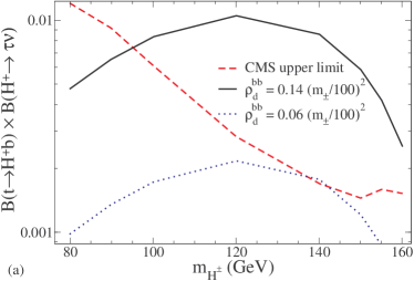
Figure 1: Left (a): CMS constraints Khachatryan:2015qxa on a charged Higgs decaying to $\tau\nu$ in the $m_{\pm}<m_{t}$ and $m_{\pm}>m_{t}$ regions. Left (a): upper limit on $B(t\to bH^{+})\cdot B(H^{+}\to\tau^{+}\nu)$ versus $m_{\pm}$ in the low mass region. Right (b): upper limit on production cross section times $B(H^{+}\to\tau^{+}\nu)$ for $m_{\pm}>180\,$GeV. Assumed values of the $\rho_{d}^{bb}$ coupling from eq. (43) are indicated.

Similarly, trying to use $\rho_{d}^{sb}$ to saturate (26) results in a branching ratio of $0.1$ for $B_{s}\to\tau^{+}\tau^{-}$. However the current limits on this decay channel are very weak, $B(B_{s}\to\tau^{+}\tau^{-})<5\%$ Grossman:1996qj ; Blake:2015tda . Using $f_{B_{s}}=0.225\,$GeV, this gives a bound on $|\rho_{d}^{sb}|$ of

$$|\rho_{d}^{sb}|<2.8\times 10^{-3}\left(m_{H}\over 100{\rm\,GeV}\right)^{2}\left|2.5\over\rho_{e}^{\tau\tau}\right|\left(B(B_{s}\to\tau^{+}\tau^{-})\over 5\times 10^{-2}\right)^{1/2}$$ (42)

It follows that we must rely upon $\rho_{d}^{bb}$ to provide at least part of the contribution to the Wilson coefficient $C_{S_{R}}$, if we insist on its central value from (26). This gives the constraint

$$|\rho_{d}^{bb}|\left(100{\rm\,GeV}\over m_{\pm}\right)^{2}\left|\rho_{e}^{\tau\tau}\over 2.5\right|\cong[0.05-0.12]$$ (43)

where the lowest value in the interval corresponds to saturating the limit (42).

With $\rho_{d}^{bb}\neq 0,$ neutral $H^{0}$ exchange also leads to the decays of the $b\bar{b}$ bound state $\chi_{b0}\to\tau^{+}\tau^{-}$ at tree level. In the SM such decays are dominantly electromagnetic, which greatly suppresses the BR of the $H^{0}$-mediated process. No bounds on leptonic decay modes of $\chi_{b0}$ are given by the Particle Data Group. For $\Upsilon$ the branching ratio for $\tau^{+}\tau^{-}$ final states is $(2.60\pm 0.10)\%$ but since it is a vector, $H^{0}$ cannot mediate the decay at tree level. Rather it proceeds at one loop with virtual $H^{0}$ and photon exchange. We estimate that it contributes less than $10^{-14}$ to the branching ratio.

Figure 2: Left (a): predicted $bb$ fusion cross section versus neutral Higgs mass for $\rho_{d}^{bb}=0.05$ and 0.11, and CMS preliminary upper limit CMS:2015mca . Right (b): allowed regions in the plane of $bb$ fusion versus $gg$ fusion cross sections, for $m_{H}=90,100\,$GeV. Theoretical predictions for $0.07\,(0.05)<\rho_{d}^{bb}<0.10$ are indicated for $m_{H}=90\,(100)\,$GeV, having negligible $\sigma(ggH)$. Figure adapted from ref. CMS:2015mca .

IV Collider constraints

We next consider LEP and LHC searches for charged and neutral Higgs bosons with decays principally into $\tau$ leptons, as predicted in our model. The charged Higgs can also have an indirect signature through its effect on the $h\to\gamma\gamma$ partial width.

IV.1 Charged Higgs searches

ATLAS Aad:2014kga and CMS Khachatryan:2015qxa have recently reported on searches for charged Higgs particles decaying into $\tau\nu$, which is the principal decay channel of $H^{\pm}$ in our model. These searches constrain our scenario in the mass ranges $m_{\pm}\in[80,\,160]$ GeV and [180, 1000] GeV, complementing previous LEP studies that excluded $m_{\pm}<95\,$GeV Abbiendi:2013hk for $H^{+}$ decaying with branching ratio of 100% into $\tau^{+}\tau^{-}$ as is the case in our model.

At low masses $m_{\pm}<160\,$GeV, the product of branching ratios $B(t\to H^{+}b)\cdot B(H^{+}\to\tau^{+}\nu)$ is bounded, since the dominant production process is through top quark decays into $H^{\pm}b$. Our model predicts that

$$B(t\to H^{+}b) \cong {(1+\eta^{2})(\rho_{d}^{bb})^{2}\over 32\pi\,m_{t}^{3}\,\Gamma_{t}}(m_{t}^{2}-m_{\pm}^{2})^{2}$$

$$B(H^{+}\to\tau\nu) = \left(1+3|\rho_{d}^{bb}/\rho_{e}^{\tau\tau}|^{2}\right)^{-1}\cong 1$$ (44)

ignoring $m_{b}$, where $\Gamma_{t}=1.4\,$GeV is the measured width of the top quark. The prediction is plotted along with the CMS limit in fig. 1(a), using the upper and lower values of $\rho_{d}^{bb}$ consistent with $R(D)$ from eq. (43). For the smaller value of $\rho_{d}^{bb}$, there is almost no restriction on the allowed mass $m_{\pm}$. The D$\not{0}$ collaboration finds a much weaker limit on $B(t\to H^{+}b)\cdot B(H^{+}\to\tau^{+}\nu)\lesssim 0.2$ in this mass range Abazov:2009aa . CDF obtains the stronger limit of 0.06 Aaltonen:2014hua , which however is still not competitive, and we do not show the Tevatron limits on the plot.

At higher masses $m_{\pm}>180\,$GeV, the $H^{\pm}$ is produced by its coupling to $tb$, either through $gg\to H^{+}\bar{t}b$ or $g\bar{b}\to H^{+}\bar{t}$. In fig. 1(b) we compare the CMS bound to the model predictions taking the lower value of $\rho_{d}^{bb}$ indicated in eq. (43)  A charged Higgs mass up to 220 GeV could be consistent with this search.

IV.2 Neutral Higgs searches

ATLAS and CMS searches for the neutral $H^{0}$ decaying to $\tau^{+}\tau^{-}$ Khachatryan:2014wca ; Aad:2014vgg ; CMS:2015mca put much stronger constraints on our model, forcing us to consider low values of both $m_{H}$ and $m_{\pm}$. Since the $\rho_{d}^{bb}$ coupling scales as $m_{\pm}^{2}$ to fit $R(D)$ (eq. (43)), $H^{0}$ typically has a larger coupling to $b$ quarks than does the SM Higgs boson. As a result, neutral $H^{0}$ production by gluon-gluon fusion Dawson:1990zj ; deFlorian:2009hc ; FGupdate , which is the dominant process for the SM Higgs, can be small compared to $bb$ fusion, leading to strong constraints on the $\sigma(bbH)$ cross section. These limits are weakest at low $m_{H}$, and also at low $m_{\pm}$ due to the scaling of $\rho_{d}^{bb}\propto m_{\pm}^{2}$.

In fig. 2(a) we plot the predictions of our model for $\sigma(bbH)$ versus $m_{H}$ (note that $B(H\to\tau^{+}\tau^{-})=1$ to a very good approximation), using the values $\rho_{d}^{bb}=0.05$ and $0.11$ suggested by eq. (43). To compute $\sigma(bbH)$, we rescaled the cross sections obtained in ref.  Trott:2010iz (which are computed for a range of $m_{H}$) by the more accurate recent results (computed at a few values of $m_{H}$) in ref. Bonvini:2015pxa . Only for the lower value of $\rho_{d}^{bb}$ are there any regions consistent with low $m_{H}$. Large values of $m_{H}$ cannot be reconciled with $\rho_{d}^{bb}$ as small as assumed ($\sim 0.1$) because of the $\rho_{d}^{bb}\propto m_{\pm}^{2}$ scaling, and the need to keep $|m_{\pm}-m_{H}|\lesssim 75\,$GeV to respect electroweak precision constraints. In the optimistic case of $\rho_{d}^{bb}=0.05$, we find an upper limit of $m_{H}<125\,$ GeV.

$m_{H}$	$90.0$	$92.5$	$95.0$	$97.5$	$100.0$
$S_{95}$	0.39	0.70	1.07	2.88	5.29

Table 2: LEP limits Schael:2006cr on the production cross section of neutral Higgs bosons from pair production $e^{+}e^{-}\to HH^{*}\to\tau^{+}\tau^{-}\tau^{+}\tau^{-}$, as a function of their mass $m_{H}$ in GeV. $S_{95}$ is the 95% c.l. upper limit on the ratio of the observed cross section to the predicted one.

The CMS search has marginal evidence for excess events at $m_{H}\cong 90-100\,$GeV, as shown in fig. 2(b). There is a slight preference for nonzero values of the two production cross sections $\sigma(ggH)$ and $\sigma(bbH)$. Our model predicts very small values of the former, $\sim 0.1\,$pb, but significant values of $\sigma(bbH)$. We show the range of predictions corresponding to $\rho_{d}^{bb}=0.05$ to $0.10$ by the vertical arrows. The lower value corresponds to saturating the limit on $B_{s}\to\tau^{+}\tau^{-}$ in eq. (42) in order to make $\rho_{d}^{bb}$ as small as possible in eq. (43). The higher value corresponds to a branching ratio for $B_{s}\to\tau^{+}\tau^{-}$ of $5\%/\sqrt{2}=3.5\%$. There is a strong correlation between $B(B_{s}\to\tau^{+}\tau^{-})$ and the possibility to satisfy the CMS constraint, leading to our prediction that $B(B_{s}\to\tau^{+}\tau^{-})$ cannot be much smaller, unless the evidence for $C_{S_{R}}$ from $R(D)$ (eq. (26)) becomes weaker.

LEP also constrained the neutral Higgs boson mass in the case of interest for our model, where $H\to\tau^{+}\tau^{-}$ almost exclusively Schael:2006cr . The statistic $S_{95}$ is defined as the 95% c.l. upper bound on the production cross section of $H^{0}$ pairs, in units of the theoretical cross section for $e^{+}e^{-}\to Z^{*}\to HH^{*}$. In the LEP analysis it was assumed that both neutral Higgs bosons are nearly degenerate, which is the same assumption that we make in our model. The pair production cross section is model-independent, since it depends only upon the SU(2) gauge interactions of the extra scalar doublet. $S_{95}$ versus $m_{H}$ is listed in table 2, showing that $m_{H}$ must be greater than $95\,$GeV. For $m_{H}\geq 100\,$GeV, the allowed cross section is more than 5 times greater than predicted, allowing for overlap between the LEP- and CMS-allowed regions.

CDF constrained the gluon fusion cross section $\sigma(ggH)$ times $B(H\to\tau^{+}\tau^{-})$ to be less than $1.7\,$pb for $m_{H}=115\,$GeV Aaltonen:2012jh , while the SM prediction is $\sigma(ggH)_{\rm SM}=1.07\,$pb Baglio:2010um . In our model $\sigma(ggH)/\sigma(ggH)_{\rm SM}=(\rho_{u}^{tt}/y_{t})^{2}\cong 2\times 10^{-3}$, far below the CDF limit. Similarly to LHC, searches for $H\to\tau^{+}\tau^{-}$ in association with $b$ quarks are more sensitive. D$\not{0}$ constrained $\sigma(bbH)\cdot B(H\to\tau^{+}\tau^{-})<0.8\,$pb for $m_{H}=115\,$GeV Chakrabarti:2011rv . The SM cross section is $\sigma(bbH)\sim 6\,$fb near this mass Dittmaier:2003ej , which gets scaled by $(\rho_{d}^{bb}/y_{b})^{2}\cong 5$ in our model, again much smaller than the limit.

In summary, $m_{\pm}\cong 100\,$GeV and $m_{H}\cong[100$-$125]\,$GeV are the favored mass ranges for satisfying the combined limits from LEP and LHC, subject to the constraints from flavor physics discussed in section III. A large value $\rho_{e}^{\tau\tau}=2.5$ is also needed, which we will show is allowed by lepton flavor universality of $Z\to\ell\ell$ decays, in section VII.1. Larger values of $m_{\pm}$ require larger values of $\rho_{d}^{bb}$ to explain $R(D)$, making it more difficult to respect searches for the neutral Higgs.

IV.3 Charged Higgs contribution to $h\to\gamma\gamma$

The charged Higgs contributes to $h\to\gamma\gamma$ at one loop, with an amplitude that is proportional to

$$A \sim 3Q_{t}^{2}A_{1/2}(\tau_{t})+A_{1}(\tau_{W})+g_{\pm}A_{0}(\tau_{\pm})$$

$$A_{0}(\tau) = -\tau^{-2}\,(\tau-{\rm arcsin}(\sqrt{\tau})^{2})$$ (45)

(see for example ref. Posch:2010hx ) where the first two terms are from the top quark and $W$ boson loop, giving $-6.5$, while $\tau_{\pm}=(m_{h}/2m_{\pm})^{2}$ and $g_{\pm}=\lambda_{1}v^{2}/(2m_{\pm}^{2})$ in the last term. The effective coupling strength is therefore $\kappa_{\gamma}=|A/6.5|\in[0.72,\,1.14]$ using constraints from ATLAS and CMS Higgs_constraints . We then find that the Higgs potential coupling $\lambda_{1}$ is bounded by

$$-0.7<\lambda_{1}<1.4$$ (46)

for $m_{\pm}=100\,$GeV.

V Charge transformation flavor ansatz

Two Higgs doublet models have had a long history of proposed mechanisms to control FCNCs, starting with that of Glashow and Weinberg Glashow:1976nt , where up and down quarks are restricted to couple to different Higgs doublets. More recent ideas include the Cheng-Sher texture Cheng:1987rs , MFV Chivukula:1987py ; D'Ambrosio:2002ex ; Cirigliano:2005ck and alignment Pich:2009sp ; Celis:2012dk . The ansatz we suggest is distinct from these, and takes the form

$$\rho_{u}^{\dagger}V=\eta\,U\,V\rho_{d}$$ (47)

where $\eta\lesssim 1$ and $U$ is a diagonal unitary matrix, whose first element is $U_{11}=-1$, while the second is $U_{22}=+1$. The third element $U_{33}$ is not yet determined by experimental constraints. We note that if $U_{33}\cong-1$ then $U$ would be special unitary. The structure (47) must of course be supplemented by a choice of entries for $\rho_{d}$ from which $\rho_{u}$ can be computed, or vice versa.

Let us comment on the general utility of this ansatz for the $B$ decays of interest. The signs chosen for $U_{11}$ and $U_{22}$ are such that the relations (28,31) are satisfied. The effect of the sign difference between $U_{11}$ and $U_{22}$ can be understood by using (47) to eliminate $\rho_{u}^{\dagger}V$ from the charged current interactions of the quarks with $H^{+}$, which then take the form

$${\cal L}=-H^{+}\bar{u}_{i}\,(P_{\scriptscriptstyle R}-\eta\,U_{ii}P_{\scriptscriptstyle L})(V\rho_{d})_{ij}\,d_{j}+{\rm h.c.}$$ (48)

If $\eta\,U_{11}=-1$, the projection operators combine as $P_{\scriptscriptstyle R}+P_{\scriptscriptstyle L}=1$ for the coupling to up quarks, forming a pure scalar $\bar{u}b$ that cannot interpolate between the pseudoscalar $B^{+}$ meson and the vacuum, hence giving no contribution to $B\to\tau\nu$ decay. For $\eta\,U_{22}=+1$, the combination $P_{\scriptscriptstyle R}-P_{\scriptscriptstyle L}=\gamma_{5}$ is pure pseudoscalar, in agreement with the sign difference in the fit result $C^{cb}_{S_{R}}\cong-C^{cb}_{S_{L}}$ Freytsis:2015qca for $B\to D\tau\nu$.

The value of $\eta$ is independently determined by either of the two anomalous measurements. Using (26-27) and (32) respectively, we find that

$$\eta\cong\left\{{0.78,\quad R(D^{(*)})\atop 0.83,\quad B\to\tau\nu}\right.$$ (49)

It is encouraging that these two estimates are consistent within the experimental errors. We adopt the compromise $\eta=0.8$ in the following. We note that in the limit $\eta=1$, the excess in $B\to D^{(*)}\tau\nu$ is completely in the vector $D^{*}$ channel and absent from the $D$ final states, because of the parity of the $\bar{c}\gamma_{5}b$ pseudoscalar coupling. By letting $\eta\neq 1$, this charged current coupling acquires a scalar component interpolating to pseudoscalar $D$ final states as well. The current data are consistent with most of the anomaly being in the $D^{*}$ channel since the error bars are smaller there (see table 1).

The relation (47) at first sight looks peculiar, since it relates two flavor symmetry breaking effects, associated with quarks of opposite charges. For convenience we give it the name of “charge transformation” (CT) mechanism. In section X we will show that such a structure can reasonably arise from a more fundamental theory of flavor. For now we will take it as a working hypothesis and check whether it is sufficient to help control FCNC’s, in conjunction with some specific choices of $\rho_{d}$ couplings.

In section VIII we will allow for all elements of $\rho_{d}$ to be nonzero, consistent with a wide variety of experimental constraints. Here we make the approximation of real-valued $\rho_{d}$ (as well as CKM matrix) so that there are only nine parameters in $\rho_{d}$. The fact that there exists a solution that can satisfy many more than nine constraints (not all of which are upper bounds because of the anomalies) is striking. Moreover we will show that there is no need for fine tuning of the parameters.

VI FCNC constraints: meson mixing

Although the anomalies in question can be accounted for with only the $\rho_{d}^{bb}$ element dominating in $\rho_{d}$ (and $\rho_{d}^{sb}\sim 0.02\,\rho_{d}^{bb}$), naturalness demands that we consider nonvanishing values of the other entries. Neutral meson mixing ($K^{0}$-$\bar{K}^{0}$, $D^{0}$-$\bar{D}^{0}$, $B^{0}$-$\bar{B}^{0}$, $B_{s}$-$\bar{B}_{s}$) provides strong constraints on their sizes. In this section we determine the tree-level and one-loop predictions of the model in the presence of general couplings.

VI.1 Neutral meson mixing: generalities

The new Higgs bosons induce contributions to neutral meson oscillations. At the quark level, they can be described by an effective Hamiltonian in which the bosons have been integrated out. In general it can contain a number of operators with different Lorentz and color structure. Even though tree-level exchanges only produce two of these operators, at one loop two additional ones are also generated.

The most general effective Hamiltonian for neutral meson mixing is

$$H=\sum_{ij}\left(\sum_{k=1,5}C^{ij}_{k}Q^{ij}_{k}+\sum_{k=1,3}\tilde{C}^{ij}_{k}\tilde{Q}^{ij}_{k}\right),$$ (50)

where the flavor indices run over $ij=sd,cu,bs,bd$ (also denoted $K$, $D$, $B_{s}$, $B_{d}$ respectively) and the operators are

$$Q_{1}^{ij} = (\bar{q}_{L,i}^{\alpha}\gamma^{\mu}q^{\alpha}_{L,j})\,(\bar{q}^{\beta}_{L,i}\gamma_{\mu}q^{\beta}_{L,j})$$ (51)

$$Q_{2}^{ij} = (\bar{q}^{\alpha}_{R,i}q^{\alpha}_{L,j})\,(\bar{q}^{\beta}_{R,i}q^{\beta}_{L,j})$$ (52)

$$Q_{3}^{ij} = (\bar{q}^{\alpha}_{R,i}q^{\beta}_{L,j})\,(\bar{q}^{\beta}_{R,i}q^{\alpha}_{L,j})$$ (53)

$$Q_{4}^{ij} = (\bar{q}^{\alpha}_{R,i}q^{\alpha}_{L,j})\,(\bar{q}^{\beta}_{L,i}q^{\beta}_{R,j})$$ (54)

$$Q_{5}^{ij} = (\bar{q}^{\alpha}_{R,i}q^{\beta}_{L,j})\,(\bar{q}^{\beta}_{L,i}q^{\alpha}_{R,j}).$$ (55)

Here $\alpha,\beta$ are colour indices, and $\tilde{Q}_{k}$ are related to $Q_{k}$ by taking $R\leftrightarrow L$. The coefficients of the latter are experimentally constrained at the same level as the ones without tildes.

Integrating out the neutral scalars, we obtain the coefficients

$$C_{2}^{ij} = \sum_{\phi=h,H,A}\frac{(y^{\dagger}_{\phi})_{ij}^{2}}{2\,m_{\phi}^{2}},$$ (56)

$$\tilde{C}_{2}^{ij} = \sum_{\phi=h,H,A}\frac{(y_{\phi})_{ij}^{2}}{2\,m_{\phi}^{2}},$$ (57)

$$C_{4}^{ij} = \sum_{\phi=h,H,A}\frac{(y^{\dagger}_{\phi})_{ij}\,(y_{\phi})_{ij}}{2\,m_{\phi}^{2}}.$$ (58)

If $H$ and $A$ are nearly degenerate as we envision in our model, then there is strong destructive interference between their contributions to $C_{2},\tilde{C}_{2}$. This can be understood in terms of the original complex fields $H\pm iA$ from the fact that the $\langle(H\pm iA)^{2}\rangle$ propagator vanishes when $H$ and $A$ are degenerate. On the other hand there is no such cancellation for $C_{4}^{ij}$, so it provides the most stringent constraints, unless one of $(y_{\phi})_{ij}$ or $(y^{\dagger}_{\phi})_{ij}$ vanishes. However naturalness favors roughly symmetric Yukawa matrices, as we will show, so that $C_{4}^{ij}$ is not suppressed in this way.

VI.2 Tree-level constraints on mixing

New tree-level contributions to neutral meson mixing are mediated by the neutral Higgs bosons. The $C_{2}^{ij}$ coefficients get contributions of opposite signs from the CP-even and odd boson exchanges. Using the mass relation (19), they can be reorganized into the form

$$\tilde{C}_{2}^{ij} = \frac{(\rho_{d}^{ij})^{2}}{2}\left[{c_{\scriptscriptstyle\beta\alpha}^{2}\over m_{h}^{2}}-{c_{\scriptscriptstyle\beta\alpha}^{2}\over m_{A}^{2}}+{c_{\scriptscriptstyle\beta\alpha}^{2}m_{h}^{2}-2\lambda_{3}v^{2}\over m_{A}^{2}\,m_{H}^{2}}\right]$$ (59)

$${C}_{2}^{ij} = \frac{(\rho_{d}^{ji*})^{2}}{2}\left[{c_{\scriptscriptstyle\beta\alpha}^{2}\over m_{h}^{2}}-{c_{\scriptscriptstyle\beta\alpha}^{2}\over m_{A}^{2}}+{c_{\scriptscriptstyle\beta\alpha}^{2}m_{h}^{2}-2\lambda_{3}v^{2}\over m_{A}^{2}\,m_{H}^{2}}\right]$$

The terms proportional to $c_{\scriptscriptstyle\beta\alpha}^{2}$ are negligible if $\lambda_{3}$ is not too small. Later we will find that $\lambda_{3}\cong 10^{-3}$ can be consistent with technical naturalness, so we adopt this value in what follows. For $m_{H}\cong m_{A}\cong 100\,$GeV, the constraints on the coefficients become Bona:2007vi ; Gedalia:2009kh

$$\bar{\rho}_{d}^{sd} < \left\{{1.3\cdot 10^{-4}\atop 9.3\cdot 10^{-6}}\right\},\quad\bar{\rho}_{d}^{cu}<\left\{{5.1\cdot 10^{-4}\atop 1.2\cdot 10^{-4}}\right\}$$

$$\bar{\rho}_{d}^{bd} < 1.1\cdot 10^{-3},\qquad\quad\bar{\rho}_{d}^{bs}<9.6\cdot 10^{-3}$$ (60)

where $\bar{\rho}_{d}^{ij}$ stands for either $|\rho_{d}^{ji}|$ or $|\rho_{d}^{ij}|$. For $K$ $(sd)$ and $D$ ($cu$), we show the separate limits from the real (upper) and imaginary (lower) parts of $C_{2}^{ij}$. In our fits we will impose the more stringent ones. These limits scale as $(m_{H}/100{\rm\,GeV})(\lambda_{3}/10^{-3})^{-1/2}$.

In the limit of small Higgs mixing and nearly degenerate $H$ and $A$, the $C_{4}^{ij}$ coefficients take the form

$$C_{4}^{ij}\cong{\rho_{q}^{ij}\rho_{q}^{ji*}\over m_{H}^{2}}$$ (61)

where $q=d$ for $K$, $B_{d}$, $B_{s}$ and $q=u$ for $D$ mixing. Unlike $C_{2}$, they are not suppressed by $c_{\scriptscriptstyle\beta\alpha}$ or $\lambda_{3}$. Again for $m_{H}=100\,$GeV, we have the upper limits

$$\sqrt{|\rho_{d}^{ds}\rho_{d}^{sd}|} < \left\{{6.0\cdot 10^{-6}\atop 4.2\cdot 10^{-7}}\right\},\ \sqrt{|\rho_{u}^{uc}\rho_{u}^{cu}|}<\left\{{2.4\cdot 10^{-5}\atop 1.0\cdot 10^{-5}}\right\}$$

$$\sqrt{|\rho_{d}^{db}\rho_{d}^{bd}|} < 4.6\times 10^{-5},\quad\sqrt{|\rho_{d}^{sb}\rho_{d}^{bs}|}<4.0\times 10^{-4}\quad\quad$$ (62)

They scale as $m_{H}/(100\,\rm{GeV})$. By comparison of (VI.2) and (VI.2) we see that $C_{4}$ gives more stringent constraints than $C_{2}$ if the coupling matrices $\rho_{q}^{ij}$ are symmetric, which will be approximately true in our later determination.

VI.3 One-loop contributions to mixing

At one loop, the charged and neutral Higgs bosons give contributions to neutral meson mixing that are higher order in $\rho_{u,d}$, except for loops involving $W^{\pm}$ exchange. We start with box diagrams involving the exchange of two scalars, followed by exchange of one $H^{\pm}$ and a $W$ boson. For mesons containing down-type quarks we find

$$C_{1}^{ij} = {1\over 128\pi^{2}}\left({(\rho_{d}^{\dagger}\,\rho_{d})_{ij}^{2}\over m_{\pm}^{2}}+{(\rho_{d}\,\rho_{d}^{\dagger})_{ij}^{2}\over m_{H}^{2}}\right)$$

$$\tilde{C}_{1}^{ij} = {(\rho_{d}^{\dagger}\,\rho_{d})_{ij}^{2}\over 128\pi^{2}}\left({1\over m_{\pm}^{2}}+{1\over m_{H}^{2}}\right)$$ (63)

$$C_{2}^{ij}=\tilde{C}_{2}^{ij}={\textstyle{1\over 4}}C_{4}^{ij} = [(V\rho_{d})^{\dagger}_{it}(V\rho_{d})_{tj}]^{2}{m_{t}^{2}(\ln{m_{\pm}^{2}\over m_{t}^{2}}-2)\over 64\pi^{2}\,m_{\pm}^{4}}$$

$$C_{5}^{ij} = {(\rho_{d}^{\dagger}\rho_{d})_{ij}\over 32\pi^{2}}\left({(\rho_{d}\rho_{d}^{\dagger})_{ij}\over m_{H}^{2}}+{(\rho_{d}^{\dagger}\rho_{d})_{ij}\over m_{\pm}^{2}}\right)$$

while for $D^{0}$ mesons

$$C_{1}^{uc} = {1\over 128\pi^{2}}\left({(V\rho_{d}\,\rho_{d}^{\dagger}V^{\dagger})_{uc}^{2}\over m_{\pm}^{2}}+{(V\rho_{d}^{\dagger}\,\rho_{d}V^{\dagger})_{uc}^{2}\over m_{H}^{2}}\right)$$

$$\tilde{C}_{1}^{uc} = {(V\rho_{d}\,\rho_{d}^{\dagger}V^{\dagger})_{uc}^{2}\over 128\pi^{2}}\left({1\over m_{\pm}^{2}}+{1\over m_{H}^{2}}\right)$$ (64)

$$C_{5}^{uc} = -{(V\rho_{d}\,\rho_{d}^{\dagger}V^{\dagger})_{uc}^{2}\over 32\pi^{2}\,m_{\pm}^{2}}-{(V\rho_{d}\,\rho_{d}^{\dagger}V^{\dagger})_{uc}(V\rho_{d}^{\dagger}\,\rho_{d}V^{\dagger})_{uc}\over 32\pi^{2}\,m_{H}^{2}}$$

We omit the $C_{2,4}^{uc}$ coefficients that are suppressed by $m_{b}^{2}$.

The box diagrams containing $H^{\pm}W^{\mp}$ exchange give rise to

$$C_{1}^{ij} = {g_{2}^{2}V_{tj}V^{*}_{ti}(V\rho_{d})_{tj}(V\rho_{d})^{*}_{ti}\over 128\pi^{2}\,m_{\pm}^{4}}\,m_{t}^{2}\left(\ln{m_{\pm}^{2}\over m_{t}^{2}}-2\right)$$

$$C_{4}^{ij} = {g_{2}^{2}(\rho_{d}^{\dagger})_{ij}(\rho_{d})_{ij}\over 64\pi^{2}\,m_{\pm}^{2}}$$

for down-quark type mesons, while for $D^{0}$ mesons

$$C_{4}^{uc}={g_{2}^{2}(V\rho_{d}^{\dagger}V^{\dagger})_{uc}(V\rho_{d}V^{\dagger})_{uc}\over 64\pi^{2}\,m_{\pm}^{2}}$$ (66)

and we neglect the $m_{b}^{2}$-suppressed contribution to $C_{1}^{uc}$.

These loop contributions turn out to be much smaller than the tree-level ones previously considered; in the numerical fit of section VIII they are at most a factor of $\sim 10^{-3}$ below the upper limits. But since they depend upon different combinations of the $\rho$ couplings, which are hierarchical, it was not a priori obvious that they should be negligible.

VII Rare decays and $(g-2)_{\tau}$

Our model predicts a variety of rare decays beyond those already considered in section III, and a new contribution to the anomalous magnetic moment of the $\tau$. Although they are potentially constraining, most of them turn out to be less so than tree-level meson mixing. The loop enhancement of $Z\to\tau^{+}\tau^{-}$ (and $Z\to\nu_{\tau}\bar{\nu}_{\tau}$) is the most important of these since it sets the limit on how large the $\rho_{e}^{\tau\tau}$ coupling can be, which is central to the explanation of the $\tau$ anomalies. The prediction for $\tau\to\pi^{-}\nu$ is close to the experimental limit for this decay, while the NP amplitude of $b\to s\gamma$ is the next most significant, a factor of four below the experimental limit.

Figure 3: Diagrams contributing to $Z\to\tau^{+}\tau^{-}$.

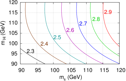
Figure 4: Contours of upper bound on $|\rho_{e}^{\tau\tau}|$ from lepton flavor universality of $Z\to\ell^{+}\ell^{-}$ decays, in the plane of neutral versus charged Higgs boson masses.

VII.1 $Z\to\tau^{+}\tau^{-}$

The coupling $\rho_{e}^{\tau\tau}$ introduces lepton universality violation in $\Gamma(Z\to\bar{\ell}\,\ell)$, when comparing $\ell=\tau$ to $\ell=e,\mu$. Such deviations are constrained by LEP, which has reported PDG

$$R_{\tau/e}=\frac{\Gamma(Z\to\tau^{+}\tau^{-})}{\Gamma(Z\to e^{+}e^{-})}=1.0019\pm 0.0032$$ (67)

The new contributions from exchange of the heavy charged and neutral scalars are shown in fig. 3. These one-loop diagrams give the effective interaction term for the right-handed component of $\tau$ coupling to $Z$:

$$\mathcal{L}_{\rm eff,\tau_{R}} = -(g_{\tau_{R}}+\delta g_{\tau_{R}})\,(\bar{\tau}_{R}\gamma_{\mu}\tau_{R})\,Z^{\mu}$$ (68)

$$g_{\tau_{R}} = g_{Z}\,s_{\scriptscriptstyle W}^{2},\quad g_{Z}={e\over c_{\scriptscriptstyle W}s_{\scriptscriptstyle W}}$$

$$\delta g_{\tau_{R}} = -{|\rho_{e}^{\tau\tau}|^{2}g_{Z}\over 32\pi^{2}}\,F_{\tau_{R}},$$

$$F_{\tau_{R}} = {\textstyle{1\over 2}}\left(F_{a}^{0}-(1-2s_{\scriptscriptstyle W}^{2})F_{b}^{0}+s_{\scriptscriptstyle W}^{2}F_{c}^{0}\right)$$

$$+ {\textstyle{1\over 2}}\left(-(1-2s_{\scriptscriptstyle W}^{2})F_{a}^{\pm}+F_{b}^{\pm}+s_{\scriptscriptstyle W}^{2}F_{c}^{\pm}\right)$$

where $c_{\scriptscriptstyle W}=\cos\theta_{W}$ and $s_{\scriptscriptstyle W}=\sin\theta_{W}$. In the limit of vanishing lepton masses, the loop integrals involving the neutral Higgs $H^{0}$ are given by

$$F_{a}^{0} = 2\int_{0}^{1}dx\int_{0}^{1-x}dy\left(\ln{(x+y)m_{H}^{2}-xy\,m_{Z}^{2}\over\mu^{2}}\right)$$

$$F_{b}^{0} = 2\int_{0}^{1}dx\int_{0}^{1-x}\!\!\!\!\!\!dy\,\left(\ln{M_{b}^{2}\over\mu^{2}}+{xy\,m_{Z}^{2}\over M_{b}^{2}}+1\right)$$

$$\left[\hbox{with}\ M_{b}^{2}=(1-x-y)\,m_{H}^{2}-xy\,m_{Z}^{2}\right]$$

$$F_{c}^{0} = 1-2\ln{m_{H}^{2}\over\mu^{2}}$$ (69)

while those involving $H^{\pm}$ (denoted by $F^{\pm}_{i}$) are the same but with $m_{H}^{2}\to m_{\pm}^{2}$. We have neglected terms of order $c_{\scriptscriptstyle\beta\alpha}^{2}$ in the Higgs mixing. Dependence on the renormalization scale $\mu$ drops out in $F_{\tau_{R}}$ and $F_{\tau_{L}}$ (below).

The analogous expressions to (68) for the couplings of $\tau_{L}$ are given by

$$\mathcal{L}_{\rm eff,\tau_{L}} = -(g_{\tau_{L}}+\delta g_{\tau_{L}})\,(\bar{\tau}_{L}\gamma_{\mu}\tau_{L})\,Z^{\mu}$$ (70)

$$g_{\tau_{L}} = -{\textstyle{1\over 2}}g_{Z}(1-2s_{\scriptscriptstyle W}^{2})$$

$$\delta g_{\tau_{L}} = -{|\rho_{e}^{\tau\tau}|^{2}g_{Z}\over 32\pi^{2}}F_{\tau_{L}},$$

$$F_{\tau_{L}} = -{\textstyle{1\over 2}}F_{a}^{0}+s_{\scriptscriptstyle W}^{2}\,F_{b}^{0}-{\textstyle{1\over 4}}(1-2s_{\scriptscriptstyle W}^{2})\,F_{c}^{0}$$

Writing $R_{\tau/e}=1+\Delta R_{\tau/e}$, the predicted value of the deviation is

$$\Delta R_{\tau/e} = 2\,{g_{\tau_{R}}\delta g_{\tau_{R}}+g_{\tau_{L}}\delta g_{\tau_{L}}\over g_{\tau_{R}}^{2}+g_{\tau_{L}}^{2}}$$

$$= {|\rho_{e}^{\tau\tau}|^{2}\over 8\pi^{2}}\left({-2s_{\scriptscriptstyle W}^{2}F_{\tau_{R}}+(1-2s_{\scriptscriptstyle W}^{2})F_{\tau_{L}}\over 4s_{\scriptscriptstyle W}^{4}+(1-2s_{\scriptscriptstyle W}^{2})^{2}}\right)$$

We take the 1$\sigma$ experimental upper limit which gives

$$-0.0013<\Delta R<0.0051$$ (72)

to obtain the upper bounds on $|\rho_{e}^{\tau\tau}|$ shown in fig. 4. (A similar calculation for more general boson masses was carried out in ref. Abe:2015oca .)

VII.2 $Z\to\nu_{\tau}\bar{\nu}_{\tau}$

Similar diagrams to those in fig. 3 contribute to the amplitude for $Z\to\nu_{\tau}\bar{\nu}_{\tau}$ decay. We find that the perturbation to the tree-level coupling in analogy to (68,70) is given by

$$\mathcal{L}_{\rm eff,\nu_{\tau}} = -(g_{\nu_{\tau}}+\delta g_{\nu_{\tau}})\,(\bar{\nu}_{\tau}\gamma_{\mu}\nu_{\tau})\,Z^{\mu}$$ (73)

$$g_{\nu_{\tau}} = {\textstyle{1\over 2}}g_{Z}$$

$$\delta g_{\nu_{\tau}} = -{|\rho_{e}^{\tau\tau}|^{2}g_{Z}\over 32\pi^{2}}F_{\nu_{\tau}},$$

$$F_{\nu_{\tau}} = {\textstyle{1\over 2}}(1-2s_{\scriptscriptstyle W}^{2})F_{a}^{\pm}+s_{\scriptscriptstyle W}^{2}\,F_{b}^{\pm}+{\textstyle{1\over 4}}\,F_{c}^{\pm}$$

The branching ratio to invisible decays is changed by

$${\Delta\Gamma_{\rm inv}\over\Gamma_{\rm inv}}={2g_{\nu_{\tau}}\delta g_{\nu_{\tau}}\over 3\,g_{\nu_{\tau}}^{2}}=-{|\rho_{e}^{\tau\tau}|^{2}F_{\nu_{\tau}}\over 24\pi^{2}}$$ (74)

For the fiducial values $\rho_{e}^{\tau\tau}=2.5$, $m_{\pm}=100{\rm\,GeV}$ that we will adopt, this leads to an increase $\Delta\Gamma_{\rm inv}=1.1{\rm\,MeV}$ in the invisible width of the $Z$. This is close to but consistent with the combined LEP upper limit $\Delta\Gamma_{\rm inv}<2{\rm\,MeV}$ ALEPH:2005ab at 95% c.l..

VII.3 $W\to\tau\nu$

Distinct from the tree-level $H^{\pm}$ decays that might have faked $W\to\tau\nu$ events at LEP, discussed in section III.3, there is an actual perturbation to the amplitude for $W\to\tau\nu$ from loops analogous to those in fig. 4. In this case, diagrams of type (b) do not contribute because they require a chirality flip leading to suppression by $m_{\tau}$, since $W$ couples only to left-handed particles. The remaining diagrams give a fractional correction to the $W\tau\nu$ coupling of

$${\delta g_{W\tau\nu}\over g_{W\tau\nu}}=-{|\rho_{e}^{\tau\tau}|^{2}\over 64\pi^{2}}\left[2F_{a}^{\pm}+{\textstyle{1\over 2}}(F_{c}^{0}+F_{c}^{\pm})\right]$$ (75)

with the loop functions in brackets evaluating to $\sim-0.1$ for the Higgs boson masses of interest. For $\rho_{e}^{\tau\tau}=2.5$, this leads to a fractional increase in the branching ratio of $0.2\%$, which is the same as the experimental error PDG . This contribution, while not enough by itself, goes in the right direction and could work in combination with the $H^{\pm}$ decays to explain the the observed excess.

VII.4 $\tau$ anomalous magnetic moment

The anomalous magnetic moment of the $\tau$ is at present only weakly constrained, $-0.052<\Delta a_{\tau}<0.013$ PDG . At one loop, the leading contribution in our model comes from neutral $H$ exchange (see for example ref. Ilisie:2015tra ),

$$\Delta a_{\tau}={|\rho_{e}^{\tau\tau}|^{2}\,m_{\tau}^{2}\over 8\pi^{2}\,m_{H}^{2}}\,F\left(m_{\tau}\over m_{H}\right)\cong 2\times 10^{-5}\left(100{\rm\,GeV}\over m_{H}\right)^{2}$$ (76)

where the loop function evaluates to $F\cong 7$. The analogous contribution from charged Higgs exchange has a much smaller loop function $\cong-0.2$.

Frequently the dominant contribution to such processes in 2HDMs is the two-loop Barr-Zee (or Bjorken-Weinberg) Bjorken:1977vt ; Barr:1985ig diagram with a top quark or other particle in one of the loops. We find that indeed the contribution from the top quark loop exceeds the one-loop contribution, giving

$$\Delta a_{\tau}={\alpha\rho_{e}^{\tau\tau}\rho_{u}^{tt}\over 8\pi^{3}}\,{\cal F}^{(1)}[(m_{t}/m_{H})^{2}]\lesssim 7\times 10^{-4}$$ (77)

where ${\cal F}^{(1)}[(m_{t}/m_{H})^{2}]=-1.14$ for $m_{H}=100\,$GeV, using the notation of ref. Ilisie:2015tra , and we took $\rho_{u}^{tt}\lesssim 0.08$ from eqs. (43,49). Although this is much smaller than the current experimental bound, it is two orders of magnitude larger than the SM prediction Burger:2015oya . We find that the other Barr-Zee diagrams are smaller, contributing $10^{-6}$ from the $\tau$ loop analogous to (77) and $10^{-5}$ from the diagrams with $t,b,\nu,H^{\pm},W^{\pm}$ in the loops ($\Delta a_{\tau}^{(4)}$ in the notation of Ilisie:2015tra ).

VII.5 Hadronic decays $\tau\to\pi^{-}\nu,\,K^{-}\nu$ and $D_{s}\to\tau\nu$

Charged Higgs exchange contributes to hadronic decays of the $\tau$, the simplest of which are $\tau\to\pi^{-}\nu$ with branching ratio $B=(10.83\pm 0.06)\%$ and $\tau\to K^{-}\nu$ with $B=(7.00\pm 0.10)\times 10^{-3}$ PDG . The amplitude for $\tau\to K^{-}\nu$ was already given in eq. (36). Using the CT flavor ansatz (47) we have $(V\rho_{d}+\rho_{u}^{\dagger}V)_{us}=(1-\eta)(V\rho_{d})_{us}$. For $\tau\to\pi^{-}\nu$, one replaces $(V\rho_{d})_{us}\to(V\rho_{d})_{ud}$, $m_{s}\to m_{d}$, $m_{K}\to m_{\pi}$ and $f_{K}\to f_{\pi}$.

In both decays, the NP contribution interferes with that of the SM. If we assume that the hint for new physics in $\tau\to K\nu$ discussed in section III.4 is just due to a statistical fluctuation, then by demanding that the extra contribution to the branching ratio does not exceed the experimental error, we find the constraints

$$|(V\rho_{d})_{us}|<7\times 10^{-4},\quad|(V\rho_{d})_{ud}|<1\times 10^{-3}$$ (78)

assuming that $\rho_{e}^{\tau\tau}=2.5$ and $m_{\pm}=100\,$GeV. We note that this constrains couplings $\rho_{d}^{qd}$ and $\rho_{d}^{qs}$ different from those ($\rho_{d}^{sb}$ and $\rho_{d}^{bb}$) required to explain the $B$ decay anomalies. In the fit to be described below (section VIII), we obtain $(V\rho_{d})_{us}=2\times 10^{-4}$, $(V\rho_{d})_{ud}=9.5\times 10^{-4}$. The NP contribution to $\tau\to\pi^{-}\nu$ is therefore close to the limit.

The matrix element for $D_{s}\to\tau\nu$ is

$${\cal M}_{D_{s}\to\tau\nu}=(1+\eta)\,{\rho_{e}^{\tau\tau}(V\rho_{d})_{cs}\,f_{D_{s}}\,m_{D_{s}}^{2}\over 2\,m_{\pm}^{2}\,(m_{c}+m_{s})}\,(\bar{u}_{\tau}P_{\scriptscriptstyle L}u_{\nu})$$ (79)

where $f_{D_{s}}=0.248\,$GeV Davies:2010ip . Using the observed branching ratio $(5.55\pm 0.24)\%$ PDG we obtain the bound

$$|(V\rho_{d})_{cd}|<1\times 10^{-3}$$ (80)

The value from our fit, $(V\rho_{d})_{cd}=-2\times 10^{-4}$, is consistent.

VII.6 $b\to s\gamma$

The off-diagonal couplings in $\rho_{d}$ and $V\rho_{d}$ introduce new contributions to $b\to s\gamma$ at one loop, which is encoded by the effective Hamiltonian Lunghi:2006hc

$$H = -{4G_{F}\over\sqrt{2}}\,V_{tb}V^{*}_{ts}\,\left(C_{7}\,{\cal O}_{7}+C_{7}^{\prime}\,{\cal O}_{7}^{\prime}\right)$$ (81)

$${\cal O}_{7}\,({\cal O}_{7}^{\prime}) = {e\,m_{b}\over 16\pi^{2}}\,\bar{s}\,(\sigma_{\mu\nu}P_{\scriptscriptstyle R(L)})\,b\,F^{\mu\nu}$$

Because of operator mixing, one should also consider the analogous operators ${\cal O}_{8}$, ${\cal O}_{8}^{\prime}$ for the chromomagnetic moments. These have been computed for type I and II 2HDMs Grinstein:1988me ; Grinstein:1990tj but not (as far as we can tell) for a general type III model. A full computation for this case might be interesting for future study. However most of the contributions appearing in our model can be inferred from the earlier calculations by transcribing the right- and left-handed couplings of the charged Higgs from the type I/II models,

$${\cal L}=(4G_{F}/\sqrt{2})^{1/2}\bar{u}\left(\xi m_{u}VP_{L}-\xi^{\prime}Vm_{d}P_{R}\right)d$$ (82)

where $m_{u,d}$ are the quark mass matrices. The dominant contributions to the one-loop charged Higgs diagrams in our model can be estimated by taking

$$\xi^{2} \to {1\over 2m_{t}^{2}G_{F}}\,{(\rho_{u}^{\dagger}V)_{ts}\over V_{ts}}\,{(\rho_{u}^{\dagger}V)_{tb}\over V_{tb}}$$ (83)

$$= 45\,U_{tt}(V\rho_{d})_{ts}(V\rho_{d})_{tb}$$

$$\xi\xi^{\prime} \to {1\over 2m_{t}\,m_{b}G_{F}}\,{(\rho_{u}^{\dagger}V)_{ts}\over V_{ts}}\,{(V\rho_{d})_{tb}\over V_{tb}}$$ (84)

$$= 2.3\times 10^{3}\,(V\rho_{d})_{ts}(V\rho_{d})_{tb}$$

in the Wilson coefficients Grinstein:1988me ; Aliev:1997uz

$$C_{7} = \xi\xi^{\prime}\left({-3y^{2}+2y\over 6(y-1)^{3}}\ln y+{3y-5y^{2}\over 12(y-1)^{2}}\right)$$

$$+ \xi^{2}\left({-3y^{3}+2y^{2}\over 12(y-1)^{4}}\ln y+{-8y^{3}-5y^{2}+7y\over 72(y-1)^{3}}\right)$$

$$C_{8} = \xi\xi^{\prime}\left({y\over 2(y-1)^{3}}\ln y+{y^{2}-3y\over 4(y-1)^{2}}\right)$$

$$+ \xi^{2}\left({y^{2}\over 4(y-1)^{4}}\ln y+{-y^{3}+5y^{2}+2y\over 24(y-1)^{3}}\right)$$

where $y=(m_{t}/m_{\pm})^{2}$. In (83) we have indicated the expressions following from our flavor ansatz (47) that involve the undetermined sign $U_{tt}=\pm 1$. In the type I/II models, $C_{7}^{\prime}$ is smaller than $C_{7}$ by a factor of $m_{s}/m_{b}$, but we do not expect that in our model since there is no suppression of the right-handed couplings by $m_{d}$. Instead, the primed coefficients are given by (VII.6) after interchanging $\rho_{u}^{\dagger}V\leftrightarrow V\rho_{d}$ in (83). With our flavor ansatz (47), this implies that $\xi^{2}$ becomes larger by the factor $1/\eta^{2}=1.56$ while $\xi\xi^{\prime}$ remains the same.

Recent constraints on $C_{7}$ and $C_{7}^{\prime}$ (by which we always mean the NP contributions) at the scale of $m_{b}$ have been determined by ref. Descotes-Genon:2015uva ,

$$C_{7}(m_{b}) \in [-0.055,\,0.02],$$

$$C^{\prime}_{7}(m_{b}) \in [-0.03,\,0.065]$$ (86)

at $2\,\sigma$. The coefficients (VII.6) evaluated at the weak scale must be run down to $m_{b}$ Grinstein:1990tj ,

$$C_{7}(m_{b}) = \eta^{16/23}C_{7}+{\textstyle{8\over 3}}(\eta^{14/23}-\eta^{16/23})C_{8}$$ (87)

$$\cong 0.6\,C_{7}+0.1\,C_{8}$$

at leading order in QCD corrections, where $\eta=\alpha_{s}(m_{W})/\alpha_{s}(m_{b})\cong 0.5$. The primed coefficients run in the analogous way. The numerical fit of section VIII yields $C_{7}(m_{b})\cong C_{7}^{\prime}(m_{b})\cong 4.9\times 10^{-3}$, four times below the limit for $C_{7}$.

There are also Barr-Zee two-loop contributions that we find to be much smaller. For example the diagram with a top quark loop and neutral $H^{0}$ exchange generates Davidson:2010xv ; Sierra:2014nqa

$$C_{7}={\sqrt{2}\,N_{c}\,Q_{b}\,Q_{t}^{2}\,\alpha\,\rho_{d}^{sb}\,\rho_{u}^{tt}\over 8\pi\,m_{b}\,m_{t}\,G_{F}\,V_{tb}\,V_{ts}}f(m_{t}^{2}/m_{H}^{2})\lesssim 10^{-4}$$ (88)

where the loop function $f(m_{t}^{2}/m_{H}^{2})\cong-1$.

VII.7 $s\to d\gamma$

For the radiative decays of lighter quarks, it is not necessarily a good approximation to assume that the top quark contribution in the loop dominates, because the relevant coupling $(V\rho_{d})_{td}$ is CKM-suppressed, and for $c\to u\gamma$ the dominant graph is from an internal $b$ quark. For these decays we content ourselves with an estimate based upon the analogous treatment of leptonic processes $\tau\to\mu\gamma$ studied in 2HDMs Davidson:2010xv , which obtains the separate contributions from neutral as well as charged Higgs exchange. Defining the operator coefficients in the effective Hamiltonian as

$${\cal H}_{\rm eff} = {Q_{s}\,e\,m_{s}\over 2}\,\bar{s}\,\sigma_{\mu\nu}(A^{sd}_{\scriptscriptstyle R}P_{\scriptscriptstyle R}+A^{sd}_{\scriptscriptstyle L}P_{\scriptscriptstyle L})b\,F^{\mu\nu}$$ (89)

we find

$$A^{sd}_{R}=(A^{sd}_{L})^{*}\!\!\! = \!\!\!\!\!\!\sum_{q=u,c,t}\!\!{Q_{q}\,m_{q}\over Q_{s}\,m_{s}}{(V\rho_{d})^{*}_{qd}(V\rho_{d})_{qs}\over 16\pi^{2}\,m_{\pm}^{2}}\,f\left(m_{\pm}\over m_{q}\right)$$

$$A^{sd}_{R}\ [A^{sd}_{L}]\! = \!\!\!\!\!\!\sum_{q=d,s,b}\!{m_{q}\over m_{s}}{\rho_{d}^{dq}\rho_{d}^{qs}\ [(\rho_{d}^{qd}\rho_{d}^{qs})^{*}]\over 16\pi^{2}\,m_{H}^{2}}\,f\left(m_{H}\over m_{q}\right)$$

$$A^{sd}_{R}\ [A^{sd}_{L}] = {\rho_{d}^{ds}\,y_{s}\,c_{\scriptscriptstyle\beta\alpha}\ [\rho_{d}^{sd*}\,y_{s}\,c_{\scriptscriptstyle\beta\alpha}]\over 16\pi^{2}\,m_{h}^{2}}\,f\left(m_{h}\over m_{s}\right)$$ (90)

where the loop function is $f(x)\cong\ln x^{2}-3/2$. Our numerical fit values of the couplings implies $|A^{sd}_{L,R}|\cong-2\times 10^{-5}\,$TeV^-2.

The dipole operator gives rise to a hadronic matrix element

$$\langle\pi^{0}|\bar{s}\sigma^{\mu\nu}d|K^{0}\rangle=\left(p_{\pi}^{\mu}p_{K}^{\nu}-p_{K}^{\mu}p_{\pi}^{\nu}\right){\sqrt{2}\,f_{T}^{K\pi}\over m_{K}+m_{\pi}}$$ (91)

with $f_{T}^{K\pi}=0.4$ Baum:2011rm . It vanishes for on-shell photons in the decay $K\to\pi\gamma$, but gives a nonvanishing contribution to leptonic modes mediated by the off-shell photon. Because $A_{L}^{sd}=A_{R}^{sd*}$, it does not contribute to the CP-violating decay $K_{L}\to\pi\ell^{+}\ell^{-}$, but it does contribute to $K_{S}\to\pi\ell^{+}\ell^{-}$ whose measured branching ratio is $(3\pm 1.5)\times 10^{-9}$ PDG .

Adapting results of ref. Becirevic:2000zi for $K_{L}$ decay, we find

$${\Delta B(K_{S}\to\pi^{0}e^{+}e^{-})\over B(K^{+}\to\pi^{0}e^{+}\nu_{e})}=\left(2\zeta e^{2}Q_{s}m_{s}\tilde{B}_{T}{\rm Re}(A_{R}^{sd})\over V_{us}G_{F}m_{K}\right)^{2}{\tau(K_{S})\over\tau(K^{+})}$$ (92)

where $\tilde{B}_{T}=1.2$ and $\zeta$ accounts for the renormalization of $A_{R}^{sd}$ between the scale $m_{H}$ and $\mu=2\,$GeV where the lattice matrix elements are computed. Assuming that the chromomagnetic moment $g_{s}\bar{d}\sigma_{\mu\nu}G^{\mu\nu}s$ gets generated with the same coefficient as the electromagnetic one $Q_{s}e\bar{d}\sigma_{\mu\nu}F^{\mu\nu}s$ at the scale $m_{H}$ and accounting for the mixing of these operators under renormalization, $\zeta=\eta^{2}(1-3\cdot 8(1-\eta^{-1}))=2.7$, where $\eta=(\alpha_{s}(m_{H})/\alpha_{s}(m_{b}))^{2/23}(\alpha_{s}(m_{b})/\alpha_{s}(\mu))^{2/25}=0.9$. Eq. (92) then gives the new physics contribution $\Delta B(K_{S}\to\pi^{0}e^{+}e^{-})=3\times 10^{-13}$, far below the measured value.

VII.8 $c\to u\gamma$

Proceeding similarly to the case of $s\to d\gamma$, the dipole operators for $c\to u\gamma$ get contributions to their coefficients given by

$$A^{cu}_{R}=(A^{cu}_{L})^{*}\!\!\! = \!\!\!\!\!\!\sum_{q=d,s,b}\!{Q_{q}\,m_{q}\over Q_{c}\,m_{c}}{(V\rho_{d})_{uq}(V\rho_{d})^{*}_{cq}\over 16\pi^{2}\,m_{\pm}^{2}}\,f\left(m_{\pm}\over m_{q}\right)$$

$$A^{bs}_{R}\ [A^{cu}_{L}]\!\! = \!\!\!\!\!\!\sum_{q=u,c,t}\!{m_{q}\over m_{c}}{\rho_{u}^{uq}\rho_{u}^{qc}\ [(\rho_{u}^{cq}\rho_{u}^{qu})^{*}]\over 16\pi^{2}\,m_{H}^{2}}\,f\left(m_{H}\over m_{q}\right)$$

$$A^{cu}_{R}\ [A^{cu}_{L}] = {\rho_{u}^{uc}\,y_{c}\,c_{\scriptscriptstyle\beta\alpha}\ [\rho_{u}^{cu*}\,y_{c}\,c_{\scriptscriptstyle\beta\alpha}]\over 16\pi^{2}\,m_{h}^{2}}\,f\left(m_{h}\over m_{c}\right)$$ (93)

The second of these (mediated by $H^{0}$ in the loop) is the largest, contributing $A_{R}^{cu}\cong 2\times 10^{-4}\,$ TeV^-2. It is difficult to put precise constraints on this quantity because of highly uncertain long-distance contributions to the observable amplitudes. Here we content ourselves with a comparison to the SM short-distance contribution, estimated to be $A^{cu}_{SM}=0.02\,G_{F}V_{us}V_{cs}/(2\sqrt{2}\pi^{2}Q_{c})\cong 2\times 10^{-3}\,$TeV^-2 Greub:1996wn ; Fajfer:2002bu . On this basis the new contribution appears to be sufficiently small, especially since the observed $\Delta c=1$ decays are dominated by the long-distance contributions.

Figure 5: Summary of meson mixing limits and predictions (dots) for the Wilson coefficients that are most constraining for our model. Allowed ranges for Im($C_{i}^{j}$) are shown as solid lines, while those for Re($C_{i}^{j}$) are dashed, for the cases where there is a distinction. The new neutral Higgs boson mass is assumed to be 115 GeV.

VIII Numerical determination of couplings

We now demonstrate numerically that it is possible to find values of the parameters consistent with all observables. We continue to assume that $m_{H}\cong m_{A}$ for the new neutral Higgs bosons, and adopt the benchmark choice $m_{H}=115\,$GeV, while taking $m_{\pm}=100\,$GeV and $\rho_{e}^{\tau\tau}=2.5$, consistent with a Higgs mixing angle $c_{\scriptscriptstyle\beta\alpha}\cong-8\times 10^{-3}$ from eq. (39). These values also satisfy collider constraints as long as $\rho_{d}^{bb},\rho_{u}^{tt}$ are sufficiently small, as we will verify, and $Z\to\ell\ell$ universality.

The best-fit values of the quark couplings $\rho_{d}$ are determined using a $\chi^{2}$ statistic that incorporates the most constraining observables (in addition to the anomalies we set out to address), namely the tree-level contributions to meson mixing. We minimize $\chi^{2}$ with respect to the elements of $\rho_{d}$, with $\rho_{u}$ determined by the CT ansatz (47), requiring that the upper limits on the Wilson coefficients $C_{4}^{M}$ not be exceeded for any meson $M$. Minimizing $\chi^{2}$ leaves some degeneracy in the fit with respect to products of the form $\rho_{q}^{ij}\rho_{q}^{ji}$, which generally must be small to satisfy the mixing constraints. We partially resolve this degeneracy by trying to enforce $|\rho_{q}^{ij}|\sim|\rho_{q}^{ji}|$ as much as possible, to avoid having matrix elements that are unnaturally small, as we will discuss in section IX.

We make the simplifying approximation of real-valued $\rho_{d}$ and $\rho_{u}$. This requires ignoring the phase of the CKM matrix as well since $\rho_{u}=\eta V\rho_{d}^{\dagger}V^{\dagger}U$ according to (47), where we take $\eta=0.8$ and $U={\rm diag}(-1,1,-1)$ for definiteness. We therefore approximate $V$ as an SO(3) matrix using eqs. (12.3-12.4) of PDG with the replacement $\bar{\rho}+i\bar{\eta}\to(\bar{\rho}^{2}+\bar{\eta}^{2})^{1/2}$, leaving for future work to incorporate phases into the analysis.

Using this fitting procedure, an example of couplings that are consistent with all constraints is

$$\rho_{d} = \left(\begin{array}[]{ccc}\phantom{-}8.3\cdot 10^{-4}&\phantom{-}1.1\cdot 10^{-7}&\phantom{-}1.3\cdot 10^{-4}\\ \phantom{-}3.8\cdot 10^{-7}&\phantom{-}7.7\cdot 10^{-4}&\phantom{-}2.8\cdot 10^{-3}\\ -1.2\cdot 10^{-5}&-2.1\cdot 10^{-5}&\phantom{-}5.5\cdot 10^{-2}\end{array}\right)$$ (97)

$$\rho_{u} = \left(\begin{array}[]{ccc}-6.6\cdot 10^{-4}&\phantom{-}3.5\cdot 10^{-6}&\phantom{-}1.4\cdot 10^{-4}\\ -2.1\cdot 10^{-5}&\phantom{-}7.8\cdot 10^{-4}&\phantom{-}1.8\cdot 10^{-3}\\ -7.6\cdot 10^{-4}&\phantom{-}4.0\cdot 10^{-3}&\phantom{-}4.4\cdot 10^{-2}\end{array}\right)$$ (101)

$$V\rho_{d} = \!\!\!\left(\begin{array}[]{rrr}8.1\cdot 10^{-4}&1.7\cdot 10^{-4}&\phantom{-}9.5\cdot 10^{-4}\\ -1.9\cdot 10^{-4}&7.5\cdot 10^{-4}&\phantom{-}5.0\cdot 10^{-3}\\ -6.8\cdot 10^{-6}&-5.3\cdot 10^{-5}&\phantom{-}5.5\cdot 10^{-2}\end{array}\right)$$ (105)

Recall that only $\rho_{d}$ is independent; $\rho_{u}$ is determined, and the charged Higgs couplings $V\rho_{d}$ are shown for convenience. Other solutions can be found with smaller values of the matrix elements not needed for the $B$ decay anomalies ($\rho_{d}^{bb}$ and $\rho_{d}^{sb}$); we have allowed the former to be nearly as large as is consistent with meson mixing constraints.

In fig. 5 we show the predicted values versus experimental limits on the magnitude of the $C_{4}^{K,D,B,B_{s}}$ Wilson coefficients corresponding to the tree-level contributions to meson mixing from $H$ exchange. For $K^{0}$ and $D^{0}$ we satisfy the more stringent constraints on the imaginary part of $C_{4}$, noting that ${\rm Im}(C_{4}^{D})$ comes from the phase of $(V\rho_{d}^{\dagger}V^{\dagger})_{uc}(V\rho_{d}^{\dagger}V^{\dagger})_{cu}^{*}\cong(V_{ub}V_{cs}^{*}|\rho_{d}^{bb}|)^{2}$, which is of the same order as the real part.

For the values of $\rho_{d}^{bb}$ and $\rho_{d}^{sb}$ given in (97), the cross section $\sigma(bbH)=1.2\,$pb for production of $H$ by $bb$ fusion, not far below the CMS upper limit of $1.8\,$pb, while the branching ratio for $B_{s}\to\tau^{+}\tau^{-}$ is predicted to be $2.9\%$, close to the current upper limit of $5\%$.

VIII.1 Including $\tau\to K\nu$ deficit

In the preceding fit we did not try to obtain the negative value of $(V\rho_{d})_{us}$ favored by eq. (37) for explaining the low $\tau\to K\nu$ determination of $V_{us}$. Doing so introduces some tension with the limit on $b\to s\gamma$. We are able to obtain $(V\rho_{d})_{us}=-1.8\times 10^{-3}$, so that $(V\rho_{d}+\rho_{u}^{\dagger}V)_{us}=(1-\eta)(V\rho_{d})_{us}=-3.6\times 10^{-4}$, close to the target value of (37), while respecting all other constraints except for a marginal violation of the $2\,\sigma$ limit on $b\to s\gamma$. The fit gives $C^{\prime}_{7}=-0.036$, which is still in the $3\,\sigma$ allowed region of ref. Descotes-Genon:2015uva .

IX One-loop corrections to couplings

A texture present in the $\rho$ matrices at tree level gets modified by loops involving products of $\rho_{u,d}$ as well as the CKM matrix $V$. Rather than estimating all possible loop corrections, it is more efficient to use a spurion analysis in which the Yukawa matrices are taken to transform under the full SU(3)${}_{u}\times$SU(3)${}_{d}\times$SU(3)_Q flavor symmetries, constructing all combinations that transform in the same way as the couplings of interest. This generates a large subset of the complete set of flavor structures that should arise from the loop corrections.

The procedure captures the contributions from loops carrying momenta between the fundamental scale down to the scale of electroweak symmetry breaking. In particular, it accounts for one-loop diagrams of the type shown in fig. 6(a,b). Diagrams of the type 6(c) require a mass insertion in the fermion line, which needs a more detailed computation. We defer such a study to the future, hoping that the terms included are reasonably representative of the full corrections. It is also possible that they give an overestimate of the true corrections, as the example of $Z\to\tau^{+}\tau^{-}$ in section VII.1 showed. In that process, the perturbation to the vertex turn out to be considerably smaller than a naive estimate of the loop diagrams suggested.

Figure 6: (a,b): One-loop corrections to couplings captured by the spurion analysis. (c) Correction requiring a chirality flip, which is not explicitly included in the spurion analysis.

It is clearest to think initially in the unbroken phase, using the couplings $\hat{y}_{u,d,e}$ and $\hat{\rho}_{u,d,e}$ of the Lagrangian (II) in the original field basis before diagonalizing $\hat{y}_{u,d,e}$. The spurious transformation properties of the Yukawa matrices under the flavor symmetries are

$$(\hat{y}_{u},\,\hat{\rho}_{u}) \rightarrow V_{Q}^{\dagger}\,(\hat{y}_{u},\,\hat{\rho}_{u})V_{u},$$

$$(\hat{y}_{d},\,\hat{\rho}_{d}) \rightarrow V_{Q}^{\dagger}\,(\hat{y}_{d},\,\hat{\rho}_{d})\,V_{d},$$

$$(\hat{y}_{e},\rho_{e}) \rightarrow V_{L}^{\dagger}\,(\hat{y}_{e},\rho_{e})\,V_{e},$$ (106)

where $V_{i}$ denotes an element of the SU(3)_i flavor subgroup.

At one loop, corrections that are cubic in the couplings are generated. Purely on the basis of the symmetries, we see that the following matrix structures would be allowed (now considering only the quark couplings):

$$\delta(\hat{y}_{u},\,\hat{\rho}_{u})\sim\left\{{\phantom{-}[(\hat{y}_{u},\,\hat{\rho}_{u})\cdot(\hat{y}_{u}^{\dagger},\,\hat{\rho}_{u}^{\dagger})]\cdot(\hat{y}_{u},\,\hat{\rho}_{u})\atop+[(\hat{y}_{d},\,\hat{\rho}_{d})\cdot(\hat{y}_{d}^{\dagger},\,\hat{\rho}_{d}^{\dagger})]\cdot(\hat{y}_{u},\,\hat{\rho}_{u})}\right.$$

$$\delta(\hat{y}_{d},\,\hat{\rho}_{d})\sim\left\{{\phantom{-}[(\hat{y}_{u},\,\hat{\rho}_{u})\cdot(\hat{y}_{u}^{\dagger},\,\hat{\rho}_{u}^{\dagger})]\cdot(\hat{y}_{d},\,\hat{\rho}_{d})\atop+[(\hat{y}_{d},\,\hat{\rho}_{d})\cdot(\hat{y}_{d}^{\dagger},\,\hat{\rho}_{d}^{\dagger})]\cdot(\hat{y}_{d},\,\hat{\rho}_{d})}\right.$$ (107)

Hence flavor symmetry alone allows 16 possible combinations as corrections to each kind of coupling. In practice, not all of these are realized by the diagrams in fig. 6, as we will explicitly check. Moreover, for a coupling to a given external Higgs field, half of these are suppressed by the small mixing angle $c_{\scriptscriptstyle\beta\alpha}$, since for example the product of the two vertices associated with a loop involving $H$ goes like $\hat{\rho}^{2}+c_{\scriptscriptstyle\beta\alpha}\hat{\rho}\hat{y}+c_{\scriptscriptstyle\beta\alpha}^{2}\hat{y}^{2}$, while those connected to $h$ give $\hat{y}^{2}+c_{\scriptscriptstyle\beta\alpha}\hat{\rho}\hat{y}+c_{\scriptscriptstyle\beta\alpha}^{2}\hat{\rho}^{2}$. Finally, it is convenient once the appropriate structures are identified to transform to the basis where the fermion mass matrices are diagonalized, and express the results in terms of $y_{i}$ (the diagonalized version of $\hat{y}_{i}$) and $\rho_{i}$. This introduces factors of the CKM matrix $V$ wherever there is a mismatch between $u$- and $d$-type indices. These come from diagrams with charged Higgs exchange.

IX.1 Corrections to quark couplings

Beyond tree level, we can no longer characterize the nonstandard couplings by just $\rho_{d}$ and $\rho_{u}$ because the simple relation between the nonstandard couplings of the light Higgs $h$ and the couplings of the heavy Higgs bosons is not preserved. The nonstandard Yukawa couplings get corrections of the form

$$\delta{\cal L}_{q} = -\sum_{q=u,d}\bar{q}_{L}\left({h\over\sqrt{2}}\,\delta y_{q,h}+H\delta\rho_{q,H}\right)q_{R}$$

$$- H^{+}\bar{u}\left(\delta(V\rho_{d})_{\pm}P_{\scriptscriptstyle R}-\delta(\rho^{\dagger}_{u}V)_{\pm}P_{\scriptscriptstyle L}\right)d+{\rm h.c.}$$

where $H=(H^{0}+iA^{0})/\sqrt{2}$. From examination of the diagrams in fig. 6(a,b), we estimate the corrections

$$\delta y_{u,h} = \epsilon_{u}^{1}\,y_{u}y_{u}^{\dagger}y_{u}+\epsilon_{u}^{2}\,\rho_{u}\rho_{u}^{\dagger}y_{u}+\epsilon_{u}^{3}\,y_{u}\rho_{u}^{\dagger}\rho_{u}$$ (109)

$$+ \epsilon_{u}^{4}\,\rho_{u}y^{\dagger}_{u}\rho_{u}+\epsilon_{u}^{5}\,V\rho_{d}y_{d}^{\dagger}V^{\dagger}\rho_{u}+\epsilon_{u}^{6}\,V\rho_{d}\rho_{d}^{\dagger}V^{\dagger}y_{u}$$

$$+ c_{\scriptscriptstyle\beta\alpha}\{\epsilon_{u}^{7}\,\rho_{u}\rho_{u}^{\dagger}\rho_{u}+\epsilon_{u}^{8}\,y_{u}\rho_{u}^{\dagger}y_{u}+\epsilon_{u}^{9}\,\rho_{u}y_{u}^{\dagger}y_{u}\$$

$$+ \epsilon_{u}^{10}\,y_{u}y_{u}^{\dagger}\rho_{u}+\epsilon_{u}^{11}\,V\rho_{d}\rho_{d}^{\dagger}V^{\dagger}\rho_{u}\}$$

$$\delta y_{d,h} = \epsilon_{d}^{1}\,y_{d}y_{d}^{\dagger}y_{d}+\epsilon_{d}^{2}\,\rho_{d}\rho_{d}^{\dagger}y_{d}+\epsilon_{d}^{3}\,y_{d}\rho_{d}^{\dagger}\rho_{d}$$ (110)

$$+ \epsilon_{d}^{4}\,\rho_{d}y^{\dagger}_{d}\rho_{d}+\epsilon_{d}^{5}\,V^{\dagger}\rho_{u}y_{u}^{\dagger}V\rho_{d}+\epsilon_{d}^{6}\,V^{\dagger}\rho_{u}\rho_{u}^{\dagger}Vy_{d}$$

$$+ c_{\scriptscriptstyle\beta\alpha}\{\epsilon_{d}^{7}\,\rho_{d}\rho_{d}^{\dagger}\rho_{d}+\epsilon_{d}^{8}\,y_{d}\rho_{d}^{\dagger}y_{d}+\epsilon_{d}^{9}\,\rho_{d}y_{d}^{\dagger}y_{d}\$$

$$+ \epsilon_{d}^{10}\,y_{d}y_{d}^{\dagger}\rho_{d}+\epsilon_{d}^{11}\,V^{\dagger}\rho_{u}\rho_{u}^{\dagger}V\rho_{d}\}$$

$$\delta y_{u,H} = c_{\scriptscriptstyle\beta\alpha}\{\eta_{u}^{1}\,y_{u}y_{u}^{\dagger}y_{u}+\eta_{u}^{2}\,\rho_{u}\rho_{u}^{\dagger}y_{u}+\eta_{u}^{3}\,y_{u}\rho_{u}^{\dagger}\rho_{u}$$ (111)

$$+ \eta_{u}^{4}\,\rho_{u}y^{\dagger}_{u}\rho_{u}+\eta_{u}^{5}\,V\rho_{d}y_{d}^{\dagger}V^{\dagger}\rho_{u}+\eta_{u}^{6}\,V\rho_{d}\rho_{d}^{\dagger}V^{\dagger}y_{u}\}$$

$$+ \eta_{u}^{7}\,\rho_{u}\rho_{u}^{\dagger}\rho_{u}+\eta_{u}^{8}\,y_{u}\rho_{u}^{\dagger}y_{u}+\eta_{u}^{9}\,\rho_{u}y_{u}^{\dagger}y_{u}\$$

$$+ \eta_{u}^{10}\,y_{u}y_{u}^{\dagger}\rho_{u}+\eta_{u}^{11}\,V\rho_{d}\rho_{d}^{\dagger}V^{\dagger}\rho_{u}$$

$$\delta y_{d,H} = c_{\scriptscriptstyle\beta\alpha}\{\eta_{d}^{1}\,y_{d}y_{d}^{\dagger}y_{d}+\eta_{d}^{2}\,\rho_{d}\rho_{d}^{\dagger}y_{d}+\eta_{d}^{3}\,y_{d}\rho_{d}^{\dagger}\rho_{d}$$ (112)

$$+ \eta_{d}^{4}\,\rho_{d}y^{\dagger}_{d}\rho_{d}+\eta_{d}^{5}\,V^{\dagger}\rho_{u}y_{u}^{\dagger}V\rho_{d}+\eta_{d}^{6}\,V^{\dagger}\rho_{u}\rho_{u}^{\dagger}Vy_{d}\}$$

$$+ \eta_{d}^{7}\,\rho_{d}\rho_{d}^{\dagger}\rho_{d}+\eta_{d}^{8}\,y_{d}\rho_{d}^{\dagger}y_{d}+\eta_{d}^{9}\,\rho_{d}y_{d}^{\dagger}y_{d}\$$

$$+ \eta_{d}^{10}\,y_{d}y_{d}^{\dagger}\rho_{d}+\eta_{d}^{11}\,V^{\dagger}\rho_{u}\rho_{u}^{\dagger}V\rho_{d}$$

$$\delta(V\rho_{d})_{\pm} = \zeta_{d}^{1}\,\rho_{u}\rho_{u}^{\dagger}V\rho_{d}+\zeta_{d}^{2}\,y_{u}\rho_{u}^{\dagger}Vy_{d}+\zeta_{d}^{3}\,y_{u}y_{u}^{\dagger}V\rho_{d}$$ (113)

$$+ \zeta_{d}^{4}\,V\rho_{d}\rho_{d}^{\dagger}\rho_{d}+\zeta_{d}^{5}\,V\rho_{d}y_{d}^{\dagger}y_{d}$$

$$+ c_{\scriptscriptstyle\beta\alpha}\{\zeta_{d}^{6}\,y_{u}\rho_{u}^{\dagger}V\rho_{d}+\zeta_{d}^{7}\,\rho_{u}\rho_{u}^{\dagger}Vy_{d}+\zeta_{d}^{8}\,\rho_{u}y_{u}^{\dagger}V\rho_{d}$$

$$+ \zeta_{d}^{9}\,V\rho_{d}\rho_{d}^{\dagger}y_{d}+\zeta_{d}^{10}\,V\rho_{d}y_{d}^{\dagger}\rho_{d}\}$$

$$\delta(\rho_{u}^{\dagger}V)_{\pm} = \zeta_{u}^{1}\,\rho_{u}^{\dagger}V\rho_{d}\rho_{d}^{\dagger}+\zeta_{u}^{2}\,y_{u}^{\dagger}V\rho_{d}y_{d}^{\dagger}+\zeta_{u}^{3}\,\rho_{u}^{\dagger}Vy_{d}y_{d}^{\dagger}$$ (114)

$$+ \zeta_{u}^{4}\,\rho_{u}^{\dagger}\rho_{u}\rho_{u}^{\dagger}V+\zeta_{u}^{5}\,y_{u}^{\dagger}y_{u}\rho_{u}^{\dagger}V$$

$$+ c_{\scriptscriptstyle\beta\alpha}\{\zeta_{u}^{6}\,\rho_{u}^{\dagger}V\rho_{d}y_{d}^{\dagger}+\zeta_{u}^{7}\,y_{u}^{\dagger}V\rho_{d}\rho_{d}^{\dagger}+\zeta_{u}^{8}\,\rho_{u}^{\dagger}Vy_{d}\rho_{d}^{\dagger}$$

$$+ \zeta_{u}^{9}\,y_{u}^{\dagger}\rho_{u}\rho_{u}^{\dagger}V+\zeta_{u}^{10}\,\rho_{u}^{\dagger}y_{u}\rho_{u}^{\dagger}V\}$$

Here the coefficients $\epsilon_{f}^{i},\,\eta_{f}^{i},\,\zeta_{f}^{i}$ are all assumed to be of order $1/16\pi^{2}$. The contributions that are suppressed by $c_{\scriptscriptstyle\beta\alpha}$ can be understood as having an odd or even number of $\rho$ or $y$ insertions respectively. For completeness, we include two corrections that exist also within the standard model, namely $\epsilon_{u,d}^{1}$. We omit them from the following analysis since they do not involve the new physics we are investigating.

To test the degree of tuning required by our numerical fit, we have computed the maximum of each of these estimates using the numerical values of the couplings in (105). The magnitude of correction to each coupling, relative to its tree-level value, and the correction responsible for the largest effect in each matrix, is given by

$$\left|{\delta\rho_{d,H}\over\rho_{d}}\right|=\left(\begin{array}[]{ccc}10^{-8}&10^{-6}&10^{-4}\\ 10^{-5}&10^{-7}&10^{-5}\\ 10^{-5}&10^{-4}&10^{-5}\end{array}\right),\quad\eta_{d}^{8}$$ (115)

$$\left|{\delta\rho_{u,H}\over\rho_{u}}\right|=\left(\begin{array}[]{ccc}10^{-7}&10^{-4}&10^{-2}\\ 10^{-4}&10^{-5}&10^{-2}\\ 10^{-2}&10^{-2}&10^{-2}\end{array}\right),\quad\!\eta_{u}^{8\mathop{\mathchar 45\relax}10}\!\!\!\!\!\!\!$$ (116)

$$\left|{\delta y_{d,h}\over c_{\scriptscriptstyle\beta\alpha}\,\rho_{d}}\right|=\left(\begin{array}[]{ccc}10^{-5}&0.2&0.2\\ 0.01&10^{-4}&10^{-2}\\ 0.1&0.6&0.2\end{array}\right),\quad\epsilon_{d}^{5}$$ (117)

$$\left|{\delta y_{u,h}\over c_{\scriptscriptstyle\beta\alpha}\,\rho_{u}}\right|=\left(\begin{array}[]{ccc}10^{-3}&0.9&2\\ 0.3&0.05&0.8\\ 0.2&0.2&0.4\end{array}\right),\quad\epsilon_{u}^{6}$$ (118)

$$\left|{\delta(V\rho_{d})_{\pm}\over V\rho_{d}}\right|=\left(\begin{array}[]{ccc}10^{-9}&10^{-7}&10^{-5}\\ 10^{-7}&10^{-7}&10^{-5}\\ 10^{-2}&10^{-2}&10^{-2}\end{array}\right),\quad\zeta_{d}^{3}$$ (119)

$$\left|{\delta(\rho_{u}^{\dagger}V)_{\pm}\over\rho_{u}^{\dagger}V}\right|=\left(\begin{array}[]{ccc}10^{-7}&10^{-5}&10^{-5}\\ 10^{-6}&10^{-5}&10^{-5}\\ 10^{-2}&10^{-2}&10^{-2}\end{array}\right),\quad\zeta_{u}^{5}$$ (120)

The most potentially worrisome elements are the corrections to $y_{d,h}^{bs}$ and $y_{u,h}^{uc}$, which can increase the tree-level contributions to $D$ and $B_{s}$ mixing mediated by light Higgs exchange. The relatively large corrections to $y_{u,h}$, namely $\delta y_{u,h}^{ut},\delta y_{u,h}^{ct}\sim 1$, are harmless since they only affect flavor-changing decays of the top quark, which are weakly constrained by observations. The other corrections can perturb the predictions for the $C_{2}$ mixing coefficients in eq. (59) by factors of at most $O(1)$. But these coefficients are less constraining than the $C_{4}$’s in our fit. The one that comes closest is $C_{2}^{B_{s}}$ which is $0.06$ of the experimental limit. Thus there is plenty of room for the tree-level couplings to receive corrections of the order we find without violating any experimental constraints.

IX.2 Lepton couplings

Unlike for the quark couplings, naturalness does not require us to turn on any significant off-diagonal elements in $\rho_{e}^{ij}$. In the absence of neutrino masses, these are not generated by loops. Charged Higgs exchange generates an off-diagonal coupling of order

$$\delta y_{e,h}^{\mu\tau}\sim{\lambda_{1}\rho_{e}^{\tau\tau}\over 16\pi^{2}}\,{m_{\mu}m_{\nu}\over m_{\pm}^{2}}$$ (121)

which is negligible. This conclusion would also remain true if we allowed for nonvanishing $\rho_{e}^{ee}$ and $\rho_{e}^{\mu\mu}$ entries (with smaller values than $\rho_{e}^{\tau\tau}$). We do not pursue a more complete exploration of the allowed leptonic couplings here.

IX.3 Higgs potential coupings

We can estimate the size of corrections to the Higgs potential couplings $\lambda_{i}$ more definitely than those for the quark couplings since the beta functions are known; see for example ref. Cline:2011mm . Our scenario requires that $\lambda_{3}\ll 1$ and $\lambda_{5}\ll 1$, whereas the other $\lambda_{i}$ could be larger. Taking $\epsilon=1/16\pi^{2}$ (which ignores possible logarithmic enhancements), the dominant contributions to the one-loop corrections are of order

$$\delta\lambda_{1} \sim \epsilon\left[(\lambda+\lambda_{6})(6\lambda_{1}+2\lambda_{2})+2\lambda_{1}^{2}+\lambda_{2}^{2}+2\lambda_{4}^{2}\right.$$

$$\quad+\left.\lambda_{1}(\rho_{e}^{\tau\tau})^{2}+3y_{t}^{2}-{\textstyle{9\over 2}}g^{2})+{\textstyle{9\over 8}}g^{4}-6y_{t}^{2}(\rho_{u}^{tt})^{2}\right]$$

$$\sim 3\cdot 10^{-2}$$

$$\delta\lambda_{2} \sim \epsilon\left[2\lambda_{2}(\lambda+\lambda_{6})+4\lambda_{1}\lambda_{2}+2\lambda_{2}^{2}+5\lambda_{4}^{2}\right.$$

$$\quad+\left.\lambda_{2}(\rho_{e}^{\tau\tau})^{2}+3y_{t}^{2}-{\textstyle{9\over 2}}g^{2})-6y_{t}^{2}(\rho_{u}^{tt})^{2}\right]$$

$$\sim 9\cdot 10^{-3}$$

$$\delta\lambda_{3} \sim \epsilon\left[{\textstyle{5\over 2}}\lambda_{4}^{2}-3y_{t}^{2}(\rho_{u}^{tt})^{2}\right]\sim 1\cdot 10^{-3}$$

$$\delta\lambda_{4} \sim \epsilon\left[\lambda_{4}(12\lambda_{6}+3\lambda_{1}+4\lambda_{2}-{\textstyle{9\over 2}}g^{2}+{\textstyle{3\over 2}}y_{t}^{2}+{\textstyle{1\over 2}}(\rho_{e}^{\tau\tau})^{2})\right.$$

$$\left.\quad-6y_{t}(\rho_{u}^{tt})^{3}\right]\quad\sim 2\cdot 10^{-2}$$

$$\delta\lambda_{5} \sim \epsilon\left[\lambda_{4}(3\lambda_{1}+2\lambda_{2})-6y_{t}^{3}\rho_{u}^{tt}\right]\sim 4\cdot 10^{-4}$$

$$\delta\lambda_{6} \sim \epsilon\left[12\lambda_{6}^{2}+\lambda_{1}^{2}+\lambda_{1}\lambda_{2}+{\textstyle{1\over 2}}\lambda_{2}^{2}+6\lambda_{4}^{2}\right.$$ (122)

$$\quad+\left.{\textstyle{9\over 16}}g^{4}-{\textstyle{9\over 2}}\lambda_{6}g^{2}-6(\rho_{u}^{tt})^{4}-2(\rho_{e}^{\tau\tau})^{4}\right]$$

$$\sim-0.5$$

where $g$ is the SU(2)_L gauge coupling and we have ignored terms involving $g^{\prime}$ (the SU(1) hypercharge) and the small $\lambda_{3}$ and $\lambda_{5}$ couplings. We have included the effect of $\rho_{e}^{\tau\tau}$ where it is not suppressed by powers of the SM tau Yukawa coupling. To obtain the numerical estimates, we chose fiducial values of the other couplings that are consistent with the assumed mass spectrum $m_{\pm}=100{\rm\,GeV}$, $m_{H}=115{\rm\,GeV}$,

$$\lambda_{1}=0.3,\quad\lambda_{2}=0.1,\quad\lambda_{4}=0.3,\quad\lambda_{6}=0.7$$ (123)

The potentially worrisome corrections are those for the smallest couplings, $\lambda_{5}\cong-6\times 10^{-4}$ using $c_{\scriptscriptstyle\beta\alpha}=-8\times 10^{-3}$ (see eq. (39)) and eq. (17), and $\lambda_{3}\cong 10^{-3}$. Comparison with the estimates in (IX.3) indicates that these values are relatively stable. Our choice of couplings in (123) allows for some accidental cancellation in $\delta\lambda_{5}$ between the bosonic and fermionic loops. Even without such a cancellation, the contribution from the top quark by itself is $\sim 3\lambda_{5}$ which requires only a mild coincidence between tree and loop contributions to obtain the desired value. Although the correction to $\lambda_{6}$ is relatively large, the phenomenology of the model is largely insensitive to its value.

IX.4 Landau pole

The large coupling $\rho_{e}^{\tau\tau}\cong 2.5$ may be expected to give rise to a Landau pole at a relatively low scale, indicating that further new physics will be required to achieve a UV complete description. To estimate this scale we consider the renormalization group equations that depend most sensitively on $\rho_{e}^{\tau\tau}$:

$${d\lambda_{6}\over d\ln\mu^{2}} \cong {1\over 16\pi^{2}}\left(12\lambda_{6}-2(\rho_{e}^{\tau\tau})^{4}\right),$$

$${d\rho_{e}^{\tau\tau}\over d\ln\mu^{2}} \cong {1\over 16\pi^{2}}(\rho_{e}^{\tau\tau})^{3}$$ (124)

Numerically solving using the initial conditions $\lambda_{6}=0.7$ (see eq. (123)) and $\rho_{e}^{\tau\tau}\cong 2.5$ at the scale $\mu=100\,$GeV, we find that the couplings diverge at $\mu\cong 55\,$TeV.

Figure 7: Moose diagram indicating the transformation properties of the SM quark fields $u_{R}$, $d_{R}$, $Q_{L}$, the heavy singlet quarks $U,D$, and the bifundamental $\Phi,\Phi_{u},\Phi_{d},M_{u},M_{d}$ under the SU(3)${}_{Q}\times$SU(3)${}_{u}\times$SU(3)_d flavor symmetry .

X Microscopic origin of CT ansatz

$H_{1}$	$H_{2}$	$\Phi$	$\Phi_{u,d}$	$M_{u,d}$	$Q_{L}$	$(u_{R},d_{R})$	$(U_{L},D_{L})$	$(U_{R},D_{R})$
$1$	$-1$	$1$	$1$	$-1$	$i$	$i$	$i$	$-i$

Table 3: $Z_{4}$ charge assignments needed for the allowed terms in the Lagrangian (125).

As an example of what kind of physics could give rise to the CT ansatz (47), we construct a model where the SU(3)${}_{Q}\times$SU(3)${}_{u}\times$SU(3)_d flavor symmetry is spontaneously broken by bifundamentals $\Phi_{u},\Phi_{d},\Phi,M_{u},M_{d}$, coupling to heavy SU(2)-singlet quarks $U_{R,L}$ and $D_{R,L}$. The charges of the fields under the flavor symmetries are shown in fig. 7. As in (II), $H_{1}$ is the SM-like Higgs field and $H_{2}$ is the new doublet, before mixing of the neutral mass eigenstates, and we take the Lagrangian at the high scale to be

$${\cal L} = {1\over\Lambda}\left(H_{1}\bar{Q}_{L}\Phi_{u}u_{R}+\tilde{H}_{1}\bar{Q}_{L}\Phi_{d}d_{R}\right)$$ (125)

$$+ \qquad\!\!H_{2}\bar{Q}_{L}U_{R}\ \quad+\tilde{H}_{2}\bar{Q}_{L}D_{R}$$

$$+ \qquad\!\!\bar{U}_{L}\Phi^{\dagger}u_{R}\qquad\!\!+\bar{D}_{L}\Phi d_{R}$$

$$+ \qquad\!\!\bar{U}_{L}M_{u}U_{R}\qquad\!\!\!\!+\bar{D}_{L}M_{d}D_{R}$$

which respects the full flavor symmetry. In table 3 we show the charge assignments under a $Z_{4}$ symmetry that allows the interactions in (125) while forbidding those with $H_{1}$ and $H_{2}$ interchanged. This symmetry gets spontaneously broken by VEVs of the bifundamental fields $M_{u,d}$, allowing for subsequent generation of the terms in the Higgs potential (II) that break the symmetry (i.e., the terms with coefficients $\lambda_{4}$ and $\lambda_{5}$). The $m_{12}^{2}H_{1}^{\dagger}H_{2}$ term that breaks it softly can be allowed from the outset, to avoid cosmological problems from domain walls.

In (125) we have not specified a fully renormalizable Lagrangian, but merely assumed that the SM-like Yukawa couplings arise from the VEVs, $\hat{y}_{u,d}=\langle\Phi_{u,d}\rangle/\Lambda$ with some large mass scale $\Lambda$. Our main interest is in the origin of the new Yukawa couplings $\hat{\rho}_{u,d}$. Assuming the simple symmetry-breaking pattern $\langle M_{d}\rangle=\langle M_{u}\rangle/\eta=M$ times the unit matrix in flavor space, after integrating out the heavy $U,D$ quarks the new Yukawas are given by $\hat{\rho}_{u}=\eta\langle\Phi^{\dagger}\rangle/M$, $\hat{\rho}_{d}=\langle\Phi\rangle/M$. However this is in the basis where $\hat{y}_{u,d}$ are not yet diagonalized. As usual, we must transform $u_{R}\to R_{u}^{\dagger}u_{R}$, $d_{R}\to R_{d}^{\dagger}d_{R}$, $u_{L}\to L_{u}^{\dagger}u_{L}$, $d_{L}\to L_{d}^{\dagger}d_{L}$. In the quark mass basis, $\rho_{u}=\eta L_{u}\langle\Phi^{\dagger}\rangle R_{u}^{\dagger}/M$, $\rho_{d}=L_{d}\langle\Phi\rangle R_{d}^{\dagger}/M$.

With these results, we can now explain the origin of the ansatz (47) by computing the two sides of that relation:

$$\eta\,UV\rho_{d} = \eta\,UL_{u}{\langle\Phi\rangle\over M}R_{d}^{\dagger}$$

$$\rho_{u}^{\dagger}V = \eta R_{u}{\langle\Phi\rangle\over M}L_{d}^{\dagger}$$ (126)

where we have used $V=L_{u}L_{d}^{\dagger}$. Equality of $\eta\,UV\rho_{d}$ and $\rho^{\dagger}_{u}V$ follows from taking

$$R_{u}=UL_{u},\quad R_{d}=L_{d}$$ (127)

One recognizes the condition $R_{d}=L_{d}$ as that which would arise if $\hat{y}_{d}$ is a symmetric matrix. The other relation $R_{u}=UL_{u}$ implies that $\hat{y}\,U$ is symmetric. This means that $\hat{y}_{u}$ splits into two pieces, one symmetric and the other antisymmetric, having no nonvanishing elements in common. For example if $U={\rm diag}(-1,1,-1)$ then $\hat{y}_{u}$ has the structure

$$\hat{y}_{u}=\left(\begin{array}[]{ccc}a&0&b\\ 0&c&0\\ b&0&d\end{array}\right)+\left(\begin{array}[]{ccc}0&e&0\\ -e&0&f\\ 0&-f&0\end{array}\right)$$ (128)

We imagine that it is possible to find a potential $V(\Phi_{u})$ whose minimum has this form. Then our ansatz, which at first sight appears contrived, can be a simple consequence of the SM-like Yukawa matrix $\hat{y}_{d}$ being symmetric in the underlying theory of flavor, while $\hat{y}_{u}$ has the pattern (128), along with the “charge transformation” bifundamental $\Phi$ whose VEV gives rise to both $\rho_{u}$ and $\rho_{d}$ simultaneously.

Our focus has been to explain the initially peculiar-looking relation between quark couplings $\rho_{u}$ and $\rho_{d}$ proposed herein, rather than the leptonic couplings $\rho_{e}$. From the flavor perspective the ansatz that $\rho_{e}$ is dominated by the single element $\rho_{e}^{\tau\tau}$ is natural since no dangerous FCNCs arise even for large values of $\rho_{e}^{\tau\tau}$. However it may be possible to accommodate $\rho_{e}$ into the UV model in the obvious manner in parallel to the quark couplings, by adding fields with interactions

$$H_{2}\bar{L}_{L}E_{R}+\bar{E}_{L}\Phi E_{R}+\bar{E}_{L}M_{e}E_{R}$$ (129)

We then predict that

$$\rho_{e}={\langle\Phi\rangle\over M_{e}}$$ (130)

assuming that the mass matrix $M_{e}$ of the heavy vector-like leptons is proportional to the unit matrix. If $\langle\Phi\rangle$ is strongly dominated by the 33 element, to explain the hypothesized leptonic couplings, this would lead to quark couplings that are also dominated by the 33 elements, and with other elements generated from these by mixing with the approximate structure of the CKM matrix. Although we do not pursue this quantitatively here, the values given in (97, 101) appear to be roughly consistent with this expectation.

XI Alternative model

It is possible to design a similar model that is less constrained by collider searches, if a light sterile neutrino $\nu_{s}$ exists. The $R(D)$ anomaly could then be explained by the new process $B\to D^{(*)}\tau\nu_{s}$ contributing to the observed decays. Similarly $B$ would get the new decay channel $B\to\tau\nu_{s}$, and $H^{\pm}\to\tau\nu_{s}$ could contaminate the $W\to\tau\nu$ signal at LEP. However the apparent rate for $\tau\to K\nu$ could only be increased in this model because of the lack of interference with the SM amplitude. This same absence would also change the fits to the Wilson coefficients for explaining $R(D)$: we estimate that

$$(C^{cb}_{S_{R}},C^{cb}_{S_{L}})=(2.14,\,-1.41)\left({\Lambda\over{\rm TeV}}\right)^{2}$$ (131)

by fitting to the decay rates, which are larger than (26-27) to compensate for the lack of interference (see appendix A). It would require a dedicated analysis to check whether this choice of coefficients significantly degrades the agreement with the decay spectra.

This scenario has the advantage that the stringent collider constraints from searches for $H\to\tau^{+}\tau^{-}$ are evaded, since now $H$ decays almost exclusively into $\nu_{s}\nu_{\tau}$. In appendix A we estimate that $m_{H}$ can become as large as $175{\rm\,GeV}$, although it is still preferable to keep $m_{\pm}$ close to $100{\rm\,GeV}$ to keep the new quark couplings small so that the predicted branching ratio for $B\to\nu_{s}\nu_{\tau}$ remains reasonably small. Even though this decay mode is expected to be less constrained than that for $B\to\tau^{+}\tau^{-}$, a theoretical understanding of the total width for $B$ in the SM compared to the experimental value limits how large it can be. We give further details about this alternative model in the appendix.

XII Conclusions

The model we have presented is admittedly unlikely, requiring coincidences of several new particles and decay modes that are just below the threshold of detection. It is much more likely that some of the experimental anomalies that motivated the model will disappear. However, if the $R(D)$ anomaly proves to be real and needs both Wilson coefficients $C^{cb}_{S_{R}},\,C^{cb}_{S_{L}}$ as indicated by several fits to the data, then our scenario seems to be the only kind of two Higgs doublet model that can be compatible with the observations. The simultaneous explanation of the other tentative anomalies in $B\to\tau\nu$, $W\to\tau\nu$ (and possibly $\tau\to K\nu$) is an added bonus that requires little extra model-building input.

The most striking prediction is that new Higgs bosons of mass $\sim 100\,$-$\,125{\rm\,GeV}$ that may have been just beyond the kinematic reach of LEP, have couplings to $b$ quarks that put the neutral one just below the current sensitivity of CMS searches. We expect that more data should soon reveal the existence of the neutral $H$ in the $\tau^{+}\tau^{-}$ channel at the LHC. A further prediction is that $B_{s}\to\tau^{+}\tau^{-}$ will be observed with a surprisingly high branching ratio of several percent. The coupling of the SM-like Higgs boson to $\tau$ should be smaller than the SM expectation, possibly having the wrong sign. Higher precision tests of $Z\to\ell\ell$ universality should start to reveal an excess in $Z\to\tau^{+}\tau^{-}$, and in the invisible $Z$ width due to extra $Z\to\nu_{\tau}\bar{\nu}_{\tau}$ decays.

The framework also suggests that other observables could be on the edge of revealing new physics: $\tau\to\pi\nu$, $b\to s\gamma$, and the neutral meson mixing amplitudes. These are less definite predictions, since we have allowed the new flavor-violating Yukawa couplings $\rho_{u,d}^{ij}$ (apart from those directly involved in explaining $R(D)$) to be nearly as large as possible while remaining consistent with experimental constraints. It is possible that they are smaller, even though there is no fundamental reason that they should be. By studying the expected size of loop contributions to the new couplings, we found that they could indeed be smaller in many cases without requiring any fine tuning.

Even if all the hints of new physics that motivated this study should disappear, some of the ideas presented here could still be of value. First, the flavor ansatz (47) reduces the arbitrariness of the new couplings, allowing us to parametrize everything in terms of $\rho_{d}$ alone. In the absence of anomalous $R(D)$, the need for sizable $\rho_{d}^{sb}$ would disappear and make a symmetric ansatz for $\rho_{d}^{ij}$ possible, further reducing the number of independent new Yukawa couplings. The primary motivation for our ansatz was to give a more definite flavor structure to the charged Higgs couplings than is generic if $\rho_{u}$ and $\rho_{d}$ are independent.

Second, we have shown that it need not be a disaster to allow generic new Yukawa couplings in two Higgs doublet models, even in the absence of any particular mechanism for suppressing FCNCs. It could be that the dangerous couplings are simply small, even though there is no symmetry principle to explain their smallness. Our model presents a counterexample to the usual concern, that small values require fine tuning. We estimated that the relative corrections from loops to the Yukawa couplings of the new Higgs fields are all less than $10^{-2}$, eqs. (115-116,119-120). The corresponding corrections to the nonstandard couplings of the SM-like Higgs (117-118) can in some cases exceed their tree-level values, but this does not lead to any significant FCNCs from $h$ exchange, since they are still small enough to remain well below constraints from meson oscillations, as long as the Higgs potential coupling $\lambda_{3}$ that controls the splitting between $m_{H}$ and $m_{A}$ is $\lesssim 10^{-3}$.

A variant model where the charged Higgs couples to $\bar{\nu}_{s}\tau_{L}$ (where $\nu_{s}$ is a light sterile neutrino) instead of $\bar{\tau}_{R}\nu_{\tau}$ is outlined in section XI and appendix A. It has greater freedom in the allowed boson masses and couplings to quarks, making it harder to rule out. Whether it can provide as good a fit to $R(D)$ requires further study.

Our original intent was to use a large $\rho_{e}^{\mu\tau}$ coupling instead of $\rho_{e}^{\tau\tau}$ to explain the hint of $h\to\mu^{\pm}\tau^{\mp}$ decays of the SM Higgs seen by CMS and ATLAS Khachatryan:2015kon ; Aad:2015gha . This turns out to be much more difficult because of the $H\to\mu^{\pm}\tau^{\mp}$ decay (with 100% branching ratio) of the new neutral boson. Even though no formal limits on $m_{H}$ with this decay channel have been published, we believe it would have been seen in the searches for $h\to\mu\tau$ of the SM Higgs, ruling out this model. Hence a further prediction of the present model is that $h\to\mu\tau$ events will prove to be a statistical fluctuation.

Acknowledgements. I thank M. Trott for inspiring and initially collaborating on this project, N. Arkani-Hamed, B. Battacharya, G. D’Ambrosio, G. Dupuis, A. Ferrari, T. Gershon, J. Griffiths, K. Kainulainen, Z. Ligeti, D. London, A. McCarn, S. Robertson, R. Sato, S. Sekula, W. Shepherd, J. Shigemitsu and B. Vachon for useful correspondence or discussions, and Mila Huskat for encouragement. I am grateful to the NBIA for its generous hospitality during this work, which is also supported by NSERC (Canada).

Appendix A Sterile neutrino model

Here we provide some details relating to the alternative model with the primary leptonic coupling of the new Higgs fields being to the left-handed lepton doublets and sterile neutrinos $\nu_{R}$,

$${\cal L}_{Y}\ni - {\bar{L}}_{L}\,\hat{y}_{\nu}\,\tilde{H}_{1}\,{\nu}_{R}-{\bar{L}}_{L}\,\hat{\rho}_{\nu}\,\tilde{H}_{2}\,{\nu}_{R}+{\rm h.c.}$$

There is also a Majorana mass term for the sterile neutrinos,

$${\textstyle{1\over 2}}(\bar{\nu}_{R}M_{R}\nu_{R}^{c}+\bar{\nu}_{R}^{c}M_{R}^{*}\bar{\nu}_{R})$$ (132)

Without loss of generality, we can work in the basis where $M_{R}$ is diagonal,

$$M_{R}={\rm diag}(M_{1},\,M_{2},\,m_{s})$$ (133)

giving a sterile neutrino $\nu_{s}$ with Majorana mass $m_{s}$, assumed to be negligibly small for having an observable effect on the decays of $B$ mesons. For simplicity we will assume that $\hat{y}_{\nu}^{i3}=0$ so that $\nu_{s}$ gets no Dirac mass from the VEV of $H_{1}$. After electroweak symmetry breaking, when $H_{1}$ has obtained the VEV $v/\sqrt{2}$, and when the heavy states are integrated out, a Majorana mass matrix is generated for the light neutrinos through the seesaw mechanism,

$$m_{\nu}={\textstyle{1\over 2}}\,v^{2}\,\hat{y}_{\nu}^{T}\hat{M}_{s}^{-1}\hat{y}_{\nu}$$ (134)

where $\hat{M}_{s}$ is the submatrix of $M_{s}$ containing the large eigenvalues. Despite having only two heavy sterile neutrinos, the seesaw mechanism works as usual to explain the small masses of the active neutrinos. The neutrino mass matrix $m_{\nu}$ gets diagonalized by the unitary transformation $\nu_{L}\to L_{\nu}\nu_{i}$ where $\nu_{i}$ denotes the mass eigenstates.

In the mass eigenbasis for the fermions and scalars, the new Yukawa couplings of neutral scalars to neutrinos take the form

$${\cal L}_{Y_{\nu}} = -{1\over\sqrt{2}}\sum_{\phi=h,H,A}y^{\nu}_{\phi i}\,\bar{\nu}_{i}\phi P_{\scriptscriptstyle R}\nu_{s}+{\rm h.c.}$$ (135)

$$y^{\nu}_{hi} = c_{\scriptscriptstyle\beta\alpha}\,\rho_{\nu}^{i},$$

$$y^{\nu}_{Hi} = -s_{\scriptscriptstyle\beta\alpha}\,\rho_{\nu}^{i},$$

$$y^{f}_{Ai} = i\rho_{\nu}^{i}$$

where $\rho_{\nu}=L_{\nu}^{\dagger}\,\hat{\rho}_{\nu}$ is a vector in the neutrino flavor space. The charged Higgs couples to the neutrinos via

$${\cal L} = -H^{+}\left[\bar{\nu}\left(U_{\nu}^{\dagger}\,\rho_{e}\right)\,P_{\scriptscriptstyle R}\,e-\bar{\nu}_{s}\,(\rho_{\nu}^{\dagger}U_{\nu})\,P_{\scriptscriptstyle L}\,e\right]$$ (136)

where $U_{\nu}=L_{\nu}^{\dagger}\,L_{e}$ is the PMNS neutrino mixing matrix. We note that if $\hat{y}_{e}$ was originally diagonal for some reason, then $\rho_{\nu}^{\dagger}U_{\nu}=\hat{\rho}_{\nu}$, so that having $\hat{\rho}_{\nu}^{i}\cong\bar{\rho}_{\nu}\delta_{i\tau}$ in the original field basis would explain why $(\rho_{\nu}^{\dagger}U_{\nu})^{\tau}$ is the dominant component of $(\rho_{\nu}^{\dagger}U_{\nu})$ despite the large mixing angles in $U_{\nu}$. We will make this assumption in the following, and for simplicity $\rho_{e}=0$, so that the charged Higgs coupling to leptons reduces to $\bar{\rho}_{\nu}H^{+}\bar{\nu}_{s}\tau_{L}+{\rm h.c.}$.

A.1 Refitting $R(D)$

To fit the $R(D)$ observations with this model, we must take into account that the new amplitude for $B\to D^{(*)}\tau\nu_{s}$ no longer interferes with the SM contribution due to the different neutrino flavor. To make the proper adjustment it is useful to parametrize the interference effect that occurs in the original model, where the ratios depend upon $x_{\pm}=(C^{cb}_{S_{R}}\pm C^{cb}_{S_{L}})/C^{cb}_{\scriptscriptstyle SM}$ with $C^{cb}_{\scriptscriptstyle SM}=2\sqrt{2}\,G_{F}V_{cb}$, as Crivellin:2012ye

$$R(D) = R(D)_{\scriptscriptstyle SM}(1+1.5\,x_{+}+1.0\,x_{+}^{2})$$

$$R(D^{*}) = R(D^{*})_{\scriptscriptstyle SM}(1+0.12\,x_{-}+0.05\,x_{-}^{2})$$ (137)

The fit (26,27) of ref. Freytsis:2015qca corresponds to $(x_{+},\,x_{-})=(0.17,\,1.66)$. In the sterile neutrino model, (A.1) is modified by omitting the terms linear in $x_{\pm}$. We find that $(x_{+},\,x_{-})\to(0.53,\,2.59)$ to compensate for this change, leading to the Wilson coefficients (131).

This rescaling ignores the effect of having no interference on the decay spectra, where the NP contribution to the amplitude multiplies $q^{2}$, the invariant lepton pair mass squared Kamenik:2008tj . Therefore the decay distribution will have a larger $q^{4}$ contribution and smaller $q^{2}$, hardening the spectrum. We leave to future work to quantify the effect of this on the fits. Here it is mainly important that $C^{cb}_{S_{R}}$ remains relatively large, which was the motivation for this study.

Then eq. (25) implies

$${C^{cb}_{S_{R}}\over\Lambda^{2}} \cong {\bar{\rho}_{\nu}^{*}(V\rho_{d})^{cb}\over m_{\pm}^{2}}\ \ \,\cong\ \ {2.1\over{\rm TeV}^{2}}$$ (138)

$${C^{cb}_{S_{L}}\over\Lambda^{2}} \cong -{\bar{\rho}_{\nu}^{*}(\rho_{u}^{\dagger}V)^{cb}\over m_{\pm}^{2}}\cong-{1.4\over{\rm TeV}^{2}}$$ (139)

Comparison with (26,27) implies that $|\bar{\rho}_{\nu}\,\rho_{u,d}|$, must be larger than in our previous determination by a factor of 1.7, while the parameter $\eta$ becomes smaller, $\eta\cong 0.67$.

Figure 8: Diagrams contributing to $Z\to\tau^{+}\tau^{-}$ in sterile neutrino model. Diagram (b) as in fig. 3 is not present.

A.2 $Z\to\tau^{+}\tau^{-}$ and $Z\to\nu_{\tau}\bar{\nu}_{\tau}$

In contrast to the case of the $\rho_{e}^{\tau\tau}$ coupling, there are only two diagrams contributing to $Z\to\tau^{+}\tau^{-}$ with the $\bar{\rho}_{\nu}$ coupling, shown in fig. 8. They involve only exchange of $H^{\pm}$, giving the effective interaction term

$$\mathcal{L}_{\rm eff,\tau} = -(g_{\tau_{L}}+\delta g_{\tau_{L}})\,(\bar{\tau}_{L}\gamma^{\mu}\tau_{L})\,Z^{\mu}$$

$$\hbox{with}\ g_{\tau_{L}} = -{\textstyle{1\over 2}}g_{Z}\,(1-2s_{\scriptscriptstyle W}^{2}),\quad g_{Z}={e\over c_{\scriptscriptstyle W}s_{\scriptscriptstyle W}}$$

$$\delta g_{\tau_{L}} = -{|\bar{\rho}_{\nu}|^{2}g_{Z}\over 32\pi^{2}}\,F_{\tau_{L}},$$

$$F_{\tau_{L}} = -{\textstyle{1\over 2}}(1-2s_{\scriptscriptstyle W}^{2})\,(F_{a}^{\pm}+{\textstyle{1\over 2}}F_{c}^{\pm})$$ (140)

Applying the limit (VII.1,72), we find

$$|\bar{\rho}_{\nu}|<2.9\left(m_{\pm}\over m_{Z}\right)^{2}$$ (141)

which is less restrictive than the analogous bound on $\rho_{e}^{\tau\tau}$. For $m_{\pm}=100{\rm\,GeV}$, we find $|\bar{\rho}_{\nu}|<3.5$, and in general the bound is closely numerically fit by $|\bar{\rho}_{\nu}|<2.9\,(m_{\pm}/m_{Z})^{2}$. Combining this with (138) puts a lower bound on the $\rho_{d}$ couplings,

$${(V\rho_{d})^{cb}}>6.1\times 10^{-3}$$ (142)

For the new contribution to $Z\to\nu_{\tau}\bar{\nu}_{\tau}$, the relevant expressions are as in (73) with the replacements $\rho_{e}^{\tau\tau}\to\bar{\rho}_{\nu}$ and

$$F_{\nu_{\tau}}={\textstyle{1\over 2}}F_{a}^{0}+{\textstyle{1\over 4}}F_{c}^{0}$$ (143)

This evaluates to be $0.5-0.6$ times smaller than $F_{\nu_{\tau}}$ in the original model, leading to a smaller contribution to the invisible $Z$ width. In the alternative model, there is also a new contribution $Z\to\nu_{s}\nu_{s}$, but it does not interfere with any SM amplitude so it is negligible.

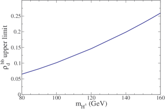
Figure 9: Upper limit on $\rho_{d}^{bb}$ inferred from CMS search Khachatryan:2015qxa for $H^{+}\to\tau\nu$ as a function of charged Higgs mass $m_{\pm}$, for $B(H^{\pm}\to\tau\nu)=1$.

A.3 Collider constraints

With $H^{0}$ decaying nearly 100% to $\nu_{s}\nu_{\tau}$, LHC constraints from neutral Higgs searches are essentially removed. We are free to take $m_{H}\cong 175{\rm\,GeV}$ for example. Such a value is just compatible with EWPD constraints (the $\rho$ parameter) on the $m_{H}$-$m_{\pm}$ mass splitting if $m_{\pm}=100{\rm\,GeV}$. Then (42) is marginally satisfied (taking it to now apply to $B_{s}\to\nu\nu$ decays) with a value that is compatible with (142) even if $\rho_{d}^{bb}=0$. In this limiting case we have

$$\bar{\rho}_{\nu}\,\rho_{d}^{sb}=0.021$$ (144)

Then $\rho_{d}^{sb}$ is the dominant coupling in $\rho_{d}$ and does the job of providing large enough $C^{cb}_{S_{R}}$ coefficient for fitting $R(D)$. With negligible $\rho_{d}^{bb}$, the production of $H^{0}$ is nullified by any other means than the subdominant electroweak $Z^{*}\to HA$ or $W^{*}\to H^{\pm}H$ processes. Moreover with $\rho_{d}^{bb}$ very small, the branching ratio $B(t\to H^{+}b)$ becomes negligible, since $\rho_{d}^{bb}\to V_{ts}\rho_{d}^{sb}$ in eq. (44), circumventing the search for charged Higgs bosons.

The combination $\bar{\rho}_{\nu}c_{\scriptscriptstyle\beta\alpha}$ is constrained by the invisible width of the Higgs boson due to $h\to\nu_{s}\nu_{\tau}$, limited to $B(h\to\nu_{s}\nu_{\tau})<36\%$ by CMS CMS:2015naa . This implies $|\bar{\rho}_{\nu}|<1.7\times{10^{-2}/|c_{\scriptscriptstyle\beta\alpha}|}$. A more stringent bound comes from the degradation of the total Higgs signal strength $\mu\cong 1.1\pm 0.1$ Higgs_constraints by invisible decays (not compensated by any increase in production), which implies $\Delta B(h\to\nu\nu)\cong 1-\mu=-0.1\pm 0.1$ Espinosa:2012vu . The $2\sigma$ upper bound implies

$$|\bar{\rho}_{\nu}|<{9\times 10^{-3}\over|c_{\scriptscriptstyle\beta\alpha}|}$$

Since (144) is compatible with both $B_{s}\to\nu\nu$ and $R(D)$, we are free to take larger mixing angle and smaller $\bar{\rho}_{\nu}$, for example $c_{\scriptscriptstyle\beta\alpha}=10^{-2}$ and $\bar{\rho}_{\nu}=0.9$, alleviating the mild naturalness tension for keeping $c_{\scriptscriptstyle\beta\alpha}$ very small, that we encountered in the model with $\rho_{e}^{\tau\tau}$.

We have the freedom to deviate from the limiting case (144) by turning on $\rho_{d}^{bb}$ again, such that (138) is fulfilled by a linear combination of $\rho_{d}^{sb}$ and $\rho_{d}^{bb}$. This reduces the branching ratio $B(B_{s}\to\nu\nu)$ and increases that of $t\to H^{+}b$ so that CMS searches for $H^{\pm}\to\tau\nu$ apply. The resulting constraint on $\rho_{d}^{bb}$, plotted in fig. 9, prevents us from attributing more than 70% of $(V\rho_{d})^{cb}$ (controlling the Wilson coefficient $C^{cb}_{S_{R}}$) to the contribution from $V_{cb}\,\rho_{d}^{bb}$. In this other limiting case, the branching ratio for $B_{s}\to\nu\nu$ is reduced to the level of $0.5\%$. Thus while the alternative version of the model is less constrained, it still predicts a significant contribution to the invisible width of $B_{s}$.

References

- (1) R. S. Chivukula and H. Georgi, Phys. Lett. B 188, 99 (1987).
- (2) G. D’Ambrosio, G. F. Giudice, G. Isidori and A. Strumia, Nucl. Phys. B 645, 155 (2002) [hep-ph/0207036].
- (3) V. Cirigliano, B. Grinstein, G. Isidori and M. B. Wise, Nucl. Phys. B 728, 121 (2005) [hep-ph/0507001].
- (4) A. L. Kagan, G. Perez, T. Volansky and J. Zupan, Phys. Rev. D 80, 076002 (2009) [arXiv:0903.1794 [hep-ph]].
- (5) J. P. Lees et al. [BaBar Collaboration], Phys. Rev. Lett. 109, 101802 (2012) [arXiv:1205.5442 [hep-ex]].
- (6) M. Huschle et al. [Belle Collaboration], arXiv:1507.03233 [hep-ex].
- (7) R. Aaij et al. [LHCb Collaboration], arXiv:1506.08614 [hep-ex].
- (8) I. Adachi et al. [Belle Collaboration], Phys. Rev. Lett. 110, no. 13, 131801 (2013) [arXiv:1208.4678 [hep-ex]].
- (9) A. Soffer, Mod. Phys. Lett. A 29, no. 07, 1430007 (2014) [arXiv:1401.7947 [hep-ex]].
- (10) A. Lusiani, M. Chrzaszcz, K. Hayasaka, H. Hayashii, J. M. Roney, B. Shwartz and S. Banerjee, Nucl. Part. Phys. Proc. 260, 32 (2015). doi:10.1016/ j.nuclphysbps.2015.02.008
- (11) S. Fajfer, J. F. Kamenik, I. Nisandzic and J. Zupan, Phys. Rev. Lett. 109, 161801 (2012) [arXiv:1206.1872 [hep-ph]].
- (12) A. Datta, M. Duraisamy and D. Ghosh, Phys. Rev. D 86, 034027 (2012) doi:10.1103/PhysRevD.86.034027 [arXiv:1206.3760 [hep-ph]]; M. Duraisamy and A. Datta, JHEP 1309, 059 (2013) doi:10.1007/JHEP09(2013)059 [arXiv:1302.7031 [hep-ph]].
- (13) A. Crivellin, C. Greub and A. Kokulu, Phys. Rev. D 86, 054014 (2012) [arXiv:1206.2634 [hep-ph]].
- (14) A. Celis, M. Jung, X. Q. Li and A. Pich, JHEP 1301, 054 (2013) [arXiv:1210.8443 [hep-ph]].
- (15) M. Tanaka and R. Watanabe, Phys. Rev. D 87, no. 3, 034028 (2013) [arXiv:1212.1878 [hep-ph]].
- (16) M. Freytsis, Z. Ligeti and J. T. Ruderman, arXiv:1506.08896 [hep-ph].
- (17) A. Crivellin, J. Heeck and P. Stoffer, arXiv:1507.07567 [hep-ph].
- (18) J. P. Lees et al. [BaBar Collaboration], Phys. Rev. D 88, no. 7, 072012 (2013) [arXiv:1303.0571 [hep-ex]].
- (19) D. Aristizabal Sierra and A. Vicente, Phys. Rev. D 90, no. 11, 115004 (2014) doi:10.1103/PhysRevD.90.115004 [arXiv:1409.7690 [hep-ph]].
- (20) K.A. Olive et al. (Particle Data Group), Chin. Phys. C38, 090001 (2014) (URL: http://pdg.lbl.gov)
- (21) Y. Omura, E. Senaha and K. Tobe, JHEP 1505, 028 (2015) [arXiv:1502.07824 [hep-ph]].
- (22) W. S. Hou, Phys. Rev. D 48, 2342 (1993).
- (23) S. Fajfer, J. F. Kamenik and I. Nisandzic, Phys. Rev. D 85, 094025 (2012) [arXiv:1203.2654 [hep-ph]].
- (24) J. Charles et al., Phys. Rev. D 91, no. 7, 073007 (2015) [arXiv:1501.05013 [hep-ph]].
- (25) R. Dermisek, arXiv:0807.2135 [hep-ph].
- (26) J.-h. Park, JHEP 0610, 077 (2006) doi:10.1088/1126-6708/2006/10/077 [hep-ph/0607280].
- (27) G. Abbiendi et al. [ALEPH and DELPHI and L3 and OPAL and LEP Collaborations], Eur. Phys. J. C 73, 2463 (2013) [arXiv:1301.6065 [hep-ex]].
- (28) Z. Czyczula [ATLAS Collaboration], Nucl. Phys. Proc. Suppl. 253-255, 180 (2014). doi:10.1016/ j.nuclphysbps.2014.09.044
- (29) The ATLAS and CMS Collaborations, ATLAS-CONF-2015-044.
- (30) H. Na, C. J. Monahan, C. T. H. Davies, R. Horgan, G. P. Lepage and J. Shigemitsu, Phys. Rev. D 86, 034506 (2012) doi:10.1103/PhysRevD.86.034506 [arXiv:1202.4914 [hep-lat]].
- (31) Y. Grossman, Z. Ligeti and E. Nardi, Phys. Rev. D 55, 2768 (1997) doi:10.1103/PhysRevD.55.2768 [hep-ph/9607473].
- (32) T. Blake, T. Gershon and G. Hiller, Ann. Rev. Nucl. Part. Sci. 65, 113 (2015) doi:10.1146/annurev-nucl-102014-022231 [arXiv:1501.03309 [hep-ex]].
- (33) G. Aad et al. [ATLAS Collaboration], JHEP 1503, 088 (2015) [arXiv:1412.6663 [hep-ex]].
- (34) V. Khachatryan et al. [CMS Collaboration], arXiv: 1508.07774 [hep-ex].
- (35) V. M. Abazov et al. [D0 Collaboration], Phys. Lett. B 682, 278 (2009) doi:10.1016/j.physletb.2009.11.016 [arXiv:0908.1811 [hep-ex]].
- (36) T. A. Aaltonen et al. [CDF Collaboration], Phys. Rev. D 89, no. 9, 091101 (2014) doi:10.1103/PhysRevD.89.091101 [arXiv:1402.6728 [hep-ex]].
- (37) V. Khachatryan et al. [CMS Collaboration], JHEP 1410, 160 (2014) doi:10.1007/JHEP10(2014)160 [arXiv: 1408.3316 [hep-ex]].
- (38) G. Aad et al. [ATLAS Collaboration], JHEP 1411, 056 (2014) doi:10.1007/JHEP11(2014)056 [arXiv:1409.6064 [hep-ex]].
- (39) CMS Collaboration [CMS Collaboration], CMS-PAS-HIG-14-029.
- (40) S. Dawson, Nucl. Phys. B 359, 283 (1991).
- (41) D. de Florian and M. Grazzini, Phys. Lett. B 674, 291 (2009) doi:10.1016/j.physletb.2009.03.033 [arXiv:0901.2427 [hep-ph]].
- (42) https://twiki.cern.ch/twiki/bin/view/LHCPhysics/ LHCHXSWGGGF (LHC Higgs Cross Section Working Group)
- (43) M. Trott and M. B. Wise, JHEP 1011, 157 (2010) [arXiv:1009.2813 [hep-ph]].
- (44) M. Bonvini, A. S. Papanastasiou and F. J. Tackmann, arXiv:1508.03288 [hep-ph].
- (45) S. Schael et al. [ALEPH and DELPHI and L3 and OPAL and LEP Working Group for Higgs Boson Searches Collaborations], Eur. Phys. J. C 47, 547 (2006) doi:10.1140/epjc/s2006-02569-7 [hep-ex/0602042].
- (46) T. Aaltonen et al. [CDF Collaboration], Phys. Rev. Lett. 108, 181804 (2012) doi:10.1103/PhysRevLett.108.181804 [arXiv:1201.4880 [hep-ex]].
- (47) J. Baglio and A. Djouadi, JHEP 1010, 064 (2010) doi:10.1007/JHEP10(2010)064 [arXiv:1003.4266 [hep-ph]].
- (48) S. Chakrabarti [D0 and CDF Collaborations], arXiv:1110.2421 [hep-ex].
- (49) S. Dittmaier, M. Kramer, 1 and M. Spira, Phys. Rev. D 70, 074010 (2004) doi:10.1103/PhysRevD.70.074010 [hep-ph/0309204].
- (50) P. Posch, Phys. Lett. B 696, 447 (2011) doi:10.1016/ j.physletb.2011.01.003 [arXiv:1001.1759 [hep-ph]].
- (51) S. L. Glashow and S. Weinberg, Phys. Rev. D 15, 1958 (1977).
- (52) T. P. Cheng and M. Sher, Phys. Rev. D 35, 3484 (1987).
- (53) A. Pich and P. Tuzon, Phys. Rev. D 80, 091702 (2009) [arXiv:0908.1554 [hep-ph]].
- (54) M. Bona et al. [UTfit Collaboration], JHEP 0803, 049 (2008) [arXiv:0707.0636 [hep-ph]].
- (55) O. Gedalia, Y. Grossman, Y. Nir and G. Perez, Phys. Rev. D 80, 055024 (2009) [arXiv:0906.1879 [hep-ph]].
- (56) T. Abe, R. Sato and K. Yagyu, JHEP 1507, 064 (2015) [arXiv:1504.07059 [hep-ph]].
- (57) S. Schael et al. [ALEPH and DELPHI and L3 and OPAL and SLD and LEP Electroweak Working Group and SLD Electroweak Group and SLD Heavy Flavour Group Collaborations], Phys. Rept. 427, 257 (2006) doi:10.1016/j.physrep.2005.12.006 [hep-ex/0509008].
- (58) V. Ilisie, JHEP 1504, 077 (2015) doi:10.1007/ JHEP04(2015)077 [arXiv:1502.04199 [hep-ph]].
- (59) J. D. Bjorken and S. Weinberg, Phys. Rev. Lett. 38, 622 (1977).
- (60) S. M. Barr and A. Zee, Phys. Rev. Lett. 55, 2253 (1985).
- (61) F. Burger, G. Hotzel, K. Jansen and M. Petschlies, arXiv:1501.05110 [hep-lat].
- (62) C. T. H. Davies, C. McNeile, E. Follana, G. P. Lepage, H. Na and J. Shigemitsu, Phys. Rev. D 82, 114504 (2010) doi:10.1103/PhysRevD.82.114504 [arXiv:1008.4018 [hep-lat]].
- (63) E. Lunghi and J. Matias, JHEP 0704, 058 (2007) [hep-ph/0612166].
- (64) B. Grinstein, R. P. Springer and M. B. Wise, Nucl. Phys. B 339, 269 (1990). doi:10.1016/0550-3213(90)90350-M
- (65) B. Grinstein, M. J. Savage and M. B. Wise, Nucl. Phys. B 319, 271 (1989). doi:10.1016/0550-3213(89)90078-3
- (66) T. M. Aliev, G. Hiller and E. O. Iltan, Nucl. Phys. B 515, 321 (1998) doi:10.1016/S0550-3213(98)00018-2 [hep-ph/9708382].
- (67) S. Descotes-Genon, L. Hofer, J. Matias and J. Virto, arXiv:1510.04239 [hep-ph].
- (68) S. Davidson and G. J. Grenier, Phys. Rev. D 81, 095016 (2010) [arXiv:1001.0434 [hep-ph]].
- (69) I. Baum, V. Lubicz, G. Martinelli, L. Orifici and S. Simula, Phys. Rev. D 84, 074503 (2011) [arXiv:1108.1021 [hep-lat]].
- (70) D. Becirevic et al. [SPQcdR Collaboration], Phys. Lett. B 501, 98 (2001) [hep-ph/0010349].
- (71) C. Greub, T. Hurth, M. Misiak and D. Wyler, Phys. Lett. B 382, 415 (1996) [hep-ph/9603417].
- (72) S. Fajfer, A. Prapotnik, S. Prelovsek, P. Singer and J. Zupan, Nucl. Phys. Proc. Suppl. 115, 93 (2003) [hep-ph/0208201].
- (73) J. M. Cline, K. Kainulainen and M. Trott, JHEP 1111, 089 (2011) [arXiv:1107.3559 [hep-ph]].
- (74) V. Khachatryan et al. [CMS Collaboration], Phys. Lett. B 749, 337 (2015) [arXiv:1502.07400 [hep-ex]].
- (75) G. Aad et al. [ATLAS Collaboration], arXiv:1508.03372 [hep-ex].
- (76) J. F. Kamenik and F. Mescia, Phys. Rev. D 78, 014003 (2008) doi:10.1103/PhysRevD.78.014003 [arXiv:0802.3790 [hep-ph]].
- (77) CMS Collaboration [CMS Collaboration], CMS-PAS-HIG-15-012.
- (78) J. R. Espinosa, M. Muhlleitner, C. Grojean and M. Trott, JHEP 1209, 126 (2012) [arXiv:1205.6790 [hep-ph]].