TIFR/TH/15-36

Thermalization in 2D critical quench and UV/IR mixing

Gautam Mandal, Shruti Paranjape, and Nilakash Sorokhaibam

Department of Theoretical Physics

Tata Institute of Fundamental Research, Mumbai 400005, India.

Abstract

We consider quantum quenches in models of free scalars and fermions with a generic time-dependent mass $m(t)$ that goes from $m_{0}$ to zero. We prove that, as anticipated in MSS [1], the post-quench dynamics can be described in terms of a state of the generalized Calabrese-Cardy form $|\psi\rangle$= $\exp[-\kappa_{2}H-\sum_{n>2}^{\infty}\kappa_{n}W_{n}]|\hbox{Bd}\rangle$. The $W_{n}$ ($n=2,3,...$, $W_{2}=H$) here represent the conserved $W_{\infty}$ charges and $|\hbox{Bd}\rangle$ represents a conformal boundary state. Our result holds irrespective of whether the pre-quench state is a ground state or a squeezed state, and is proved without recourse to perturbation expansion in the $\kappa_{n}$’s as in MSS. We compute exact time-dependent correlators for some specific quench protocols $m(t)$. The correlators explicitly show thermalization to a generalized Gibbs ensemble (GGE), with inverse temperature $\beta=4\kappa_{2}$, and chemical potentials $\mu_{n}=4\kappa_{n}$. In case the pre-quench state is a ground state, it is possible to retrieve the exact quench protocol $m(t)$ from the final GGE, by an application of inverse scattering techniques. Another notable result, which we interpret as a UV/IR mixing, is that the long distance and long time (IR) behaviour of some correlators depends crucially on all $\kappa_{n}$’s, although they are highly irrelevant couplings in the usual RG parlance. This indicates subtleties in RG arguments when applied to non-equilibrium dynamics.

1 Introduction and Summary

The dynamics of systems undergoing a quantum quench has been extensively studied in recent years [2]. In a quantum quench, some parameter of the Hamiltonian changes over a brief period of time. The initial wavefunction in the pre-quench phase, whether it is a ground state or otherwise, typically evolves to a non-stationary state, which then evolves by the post-quench Hamiltonian which is time-independent. An important question in such dynamics is whether correlators equilibrate at long times, and if so, whether the equilibrium is described by a thermal ensemble or otherwise [2, 3, 4]. With the advent of AdS/CFT, the issue of thermalization has assumed additional significance as it maps to the subject of gravitational collapse to a black hole [5, 6]. This has given rise to an extensive literature on holographic thermalization (see, e.g. [7, 8, 9], for some of the early papers on the subject). This correspondence has a direct bearing on the issue of universality of thermalization since a collapse to a black hole state is also typically associated with loss of most memory of the collapsing matter. In this paper, we will find that the final equilibrium state is characterized by an infinite number of thermodynamic parameters (chemical potentials) which retain a partial memory of the quench protocol; in the holographic dual, this corresponds to retention of memory by the final black hole of the collapsing matter.

A significant step in proving thermalization in a closed 2D system was taken in a recent paper (MSS) [1] (similar results have subsequently appeared in [10]). MSS considered 1+1 dimensional quenches, ending with a critical post-quench Hamiltonian and made the following assumptions:
(a) the post-quench wavefunction is of the generalized Calabrese-Cardy (gCC) form

$$|\psi\rangle_{gCC}=|\psi(\kappa_{2},\{\kappa_{n}\})\rangle\equiv\exp[-\kappa_{2}H-\sum_{n>2}\kappa_{n}W_{n}]|Bd\rangle$$ (1)

where $W_{n}$ are additional conserved charges in the system (the results are valid even without the additional charges present in the system). It was assumed that the charges are obtained from local currents. Below, for specificity, we will assume that the system is integrable, with a ${\mathbb{W}}_{\infty}$ algebra and the $W_{n}$, $n=2,3,...$ ($W_{2}=H$) are ${\mathbb{W}}_{\infty}$ charges.
(b) The spectrum of conformal dimensions in the post-quench critical theory has a gap.
(c) The dimensionless parameters $\tilde{\kappa}_{n}=\kappa_{n}/\kappa_{2}^{n-1},n>2$ are small and can be treated perturbatively.
(d) The size $l$ of the interval is small compared to $\kappa_{2}$.

With these assumptions in place, MSS proved that the reduced density matrix of an interval of size $l$ in the state (1) asymptotes to that in a GGE , defined by

$$\rho_{{}_{\rm GGE}}=\frac{e^{-\beta H-\sum_{n=3}^{\infty}\mu_{n}W_{n}}}{Z},\kern 5.0pt\beta=4\kappa_{2},\;\mu_{n}=4\kappa_{n},n>2$$ (2)

with a relaxation rate given by

$$\gamma=\frac{2\pi}{\beta}\left[\Delta+\sum_{n=3}^{\infty}\tilde{\mu}_{n}Q_{n}+O({\tilde{\mu}_{n}}^{2})\right],\kern 3.0pt\tilde{\mu}_{n}\equiv\frac{\mu_{n}}{\beta^{n-1}},$$ (3)

where $\Delta,Q_{n}$ are determined by the conformal dimension and other ${\mathbb{W}}_{\infty}$ charges of the most relevant operator of the CFT (by assumption (b) above, $\Delta>0$). A consequence of this result is that the expectation value of an arbitrary string of local operators, which can be enclosed in an interval of length $l$, exponentially thermalizes to its expectation value in the GGE.

One of the motivations of the present work is to extend the proof of thermalization, without making the assumptions made in MSS, in theories of free scalars or fermions with a time-dependent mass $m(t)$ quenched to $m=0$. We allow for nontrivial pre-quench states.

We proceed in two ways:

• We consider arbitrary quench protocols $m(t)$ and arbitrary squeezed states as pre-quench states (including the ground state) and show that the quench leads to a wavefunction of the gCC form. This proves the main ansatz of MSS (assumption (a) above). We also show that by judiciously choosing the pre-quench states one can satisfy the perturbative assumption (c). Thus, for theories satisfying (b) and, for intervals satisfying (d), thermalization follows from first principles, using the results of MSS.

• For specific quench protocols, but with arbitrary pre-quench states as above, we compute exact time-dependent correlators, and explicitly show thermalization of one- and two-point functions, without making any of the assumptions of MSS.

One of the technical advances in this paper is the use of non-trivial pre-quench states, which we take to be squeezed states. The motivation for considering this class of states is that besides being technically accessible, these states are experimentally realizable (see, e.g. [25, 26]) and carry non-trivial quantum entanglement encoded by the squeezing function.

We list below some salient features of our analysis:

1. Memory retention by the equilibrium ensemble: By using inverse scattering methods applied to the above-mentioned auxiliary potential scattering, we are able to relate the post-quench wavefunction, in particular $\kappa_{n}$-parameters of the gCC state, to the quench protocol $m(t)$. In fact, if we start with the ground state of the pre-quench Hamiltonian, the $\kappa_{n}$ parameters completely encode $m(t)$, implying that the equilibrium ensemble specified by $\mu_{n}=4\kappa_{n}$, carries a precise memory of the quench protocol! In case we start with a squeezed state, the equilibrium ensemble remembers a combination of the quench protocol and the knowledge of the initial state.

2. UV/IR mixing (IR sensitivity to irrelevant operators): As already found in MSS, the relaxation rate of various operators (3), which govern late time dynamics, depends on all the chemical potentials $\mu_{n}$, equivalently on the $\kappa_{n}$. Now from (1) it is clear that the $\kappa_{n}$ represent perturbing a given initial state by higher dimensional (irrelevant) operators. Indeed, our computation of the exact correlators, shows that for a large class of operators, these correlators at long times and large distances, are affected by all these chemical potentials, in apparent contradiction to IR universality (this is elaborated in Section 5). This phenomenon is actually related to the memory retention mentioned above.

3. Holographic correspondence: Our results show that for a given quench protocol, a GGE with a finite number of specified chemical potentials can be obtained by taking the pre-quench state to be a suitably chosen squeezed state. By using this result and the correspondence shown in MSS between thermalization to GGE and quasinormal decay to a higher spin black hole, we infer that higher spin black holes with an arbitrary set of chemical potentials get related to thermalization of squeezed states in the field theory.

Outline: The outline and organization of the paper is as follows:

In Section 2 we consider mass quenches in a free scalar in two dimensions. We relate the dynamics to an equivalent potential scattering problem, details of which are provided in Appendix A. We find that the exact time-dependent wavefunction can be related to a Bogoliubov transform of the ‘out’ vacuum (the post-quench ground state). Using this fact we write down the exact form of the scalar propagator. These results hold for a general mass quench, including quenches from a massless to a massless theory. We find that the quenched state is always describable in terms of a gCC state (using an application of the BCH formula, as described in Appendix B). In Section 2.4 we work all of this out for a specific quench protocol (i.e. specific time dependence of the mass parameter). In Section 2.6 we consider cases where the pre-quench state is a squeezed state. We show that this gives us a large class of initial conditions, by tuning which we can prepare a quench state in the exact form $\exp[-\sum_{n}\kappa_{n}W_{n}]|D\rangle$ which has a finite number of given $\kappa_{n}$ coefficients.

In Section 3 we show how to generalize the above results to fermions.

In Section 4.1 real time Wightman correlators in a GGE are computed. In Sections 4.2 and 4.3 we work out the scalar propagator for the specific quench protocol of Section 2.4. This allows us to compute various exact correlators, starting either from a ground state or from specific quench states leading to a gCC state with a finite number of $\kappa_{n}$ parameters. We show that these correlators thermalize exponentially to a GGE; the relaxation rate is found non-perturbatively, which agrees with (3) in the perturbative regime.

In Section 5 we show that the IR behaviour of exact correlators is sensitive to all the chemical potentials even though these represent perturbation by irrelevant operators. We also show that the equilibrium ensemble remembers the quench protocol.

In Section 6 we make concluding remarks and mention some open problems. In Appendices C and D we discuss some notations and general results about bosonic and fermionic theories. In Appendix E we elaborate the precise meaning of the sudden limit, taking into account the UV cut-off of the theory.

2 Critical quench of a scalar field: general strategy

An important example of quantum quench is provided by free scalar field theories with time-dependent mass (our notations will closely follow [27, 28], which also contain an extensive reference to the relevant literature).

$$S =-\frac{1}{2}\int d^{2}x(\partial_{\mu}\phi~{}\partial^{\mu}\phi-m^{2}(t)\phi^{2})$$

$$=\frac{1}{2}\int\frac{dkdt}{2\pi}\left(|\dot{\phi}(k,t)|^{2}-(k^{2}+m^{2}(t))|\phi(k,t)|^{2}\right),\kern 5.0pt\phi(-k,t)=\phi^{*}(k,t)$$ (4)

We will always be working in the thermodynamic limit of infinite system size. The momentum integrals will be taken to be $\int^{\infty}_{-\infty}dk/2\pi$, unless otherwise specified.

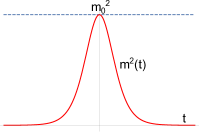
Figure 2: A mass-profile describing quantum quench from a critical Hamiltonian back to the critical Hamiltonian. Here $m^{2}(t)\xrightarrow{t\to\pm\infty}0$.

In this section we will consider a mass function $m(t)$ (this is referred to as a ‘quench protocol’) which decreases from an asymptotic value $m_{0}$ in the past to the asymptotic value $m=0$ in the future. This is called a critical quench since the mass gap vanishes following the quench. The generalization to other cases like massless to massless quench as in Figure 2 is straightforward and will be touched upon in a later section.

Because of translational symmetry, the equations of motion of various Fourier modes in (4) get decoupled, where each mode satisfies a Schrödinger-type equation:

$$-\ \frac{d^{2}}{dt^{2}}\phi(k,t)=(k^{2}+m^{2}(t))\phi(k,t)$$ (5)

From the asymptotic behaviour of the potential, it is clear that (5) admits solutions (see, e.g. [29]) which behave like plane waves at far past and far future. We will call $u_{in}(k,t)$ the solution of the wave equation which approaches a purely positive frequency solution in the past and $u_{out}(k,t)$ the solution which approaches a purely positive frequency solution in the future:

$$u_{in}\xrightarrow{t\to-\infty}\frac{e^{-i\omega_{in}t}}{\sqrt{2\omega_{in}}},\quad u_{out}\xrightarrow{t\to\infty}\frac{e^{-i\omega_{out}t}}{\sqrt{2\omega_{out}}}$$ (6)

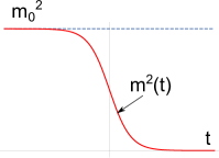
Figure 1: Mass quench from $m_{0}$ to 0.

The question of existence of the exact solutions $u_{in},u_{out}$ is essentially identical to the existence of the so-called Jost functions in the analogous Schrödinger problem, which is discussed in detail in Appendix A. The relevant properties of the Jost functions, and equivalently of the solutions $u_{in},u_{out}$, can be proved under appropriate fall-off conditions of the mass-function (to the asymptotic values) as discussed in the Appendix.

It is easy to see that the pair of solutions $u_{in}(k,t)$ and $u^{*}_{in}(-k,t)$ are independent functions (e.g. by computing the Wronskian in the far past), and hence form a basis of solutions of the second order differential equation (5). Similar remarks apply to the pair of solutions $u_{out},u^{*}_{out}$. Thus, we can write any set as a linear combination of the other; e.g.

$$u_{in}(k)=\alpha(k)u_{out}(k)+\beta(k)u^{*}_{out}(-k),\quad u_{out}(k)=\alpha^{*}(k)u_{in}(k)-\beta(k)u^{*}_{in}(-k)$$ (7)

The coefficients $\alpha,\beta$ are called Bogoliubov coefficients (our conventions here are the same as in [29]), which are determined by the mass-function $m^{2}(t)$.

Indeed, a general solution of the wave equation can be written as a linear combination of either pair:

$$\phi(k,t)=a_{in}(k)u_{in}(k,t)+a^{*}_{in}(-k)u^{*}_{in}(-k,t)=a_{out}(k)u_{out}(k,t)+a^{*}_{out}(-k)u^{*}_{out}(-k,t)$$ (8)

Here we have explicitly put in the reality condition on the scalar field $\phi(x,t)$ which translates in mixed Fourier space to $\phi^{*}(k,t)=\phi(-k,t)$.

Using the two equations above, one can find

$$a_{in}(k) =\alpha^{*}(k)a_{out}(k)-\beta^{*}(k)a^{\dagger}_{out}(-k),$$ (9)

$$a_{out}(k) =\alpha(k)a_{in}(k)+\beta^{*}(k)a^{\dagger}_{in}(-k),$$ (10)

Upon quantization, the coefficients $a_{in,out}(k)$ are treated as operators in the Fock space (with $a^{*}_{in,out}(k)$ rewritten as $a^{\dagger}_{in,out}(k)$). The specific normalizations of the $u$-functions in (6) imply that the Bogoliubov coefficients satisfy the following constraints

$$|\alpha|^{2}-|\beta|^{2}=1$$ (11)

The derivation of the above relations can be found in standard textbooks, e.g. [29], or from the analogous Schrödinger problem as in Appendix A.

2.1 General proof of the gCC ansatz [1] for the ground state

The two sets of oscillators $a_{in}(k)$ and $a_{out}(k)$ define two distinct vacua $|0,in\rangle$ and $|0,out\rangle$, defined by $a_{in}(k)|0,in\rangle=0$ and $a_{out}(k)|0,out\rangle=0$. Let us assume that we start from the ground state of the original massive theory, i.e. $|0,in\rangle$.

Using (9), we can express the in-vacuum in terms of the out-vacua as follows

$$|0,in\rangle =\exp[\frac{1}{2}\sum_{k}\gamma(k)a^{\dagger}_{out}(k)a^{\dagger}_{out}(-k)]|0,out\rangle,$$ (12)

where

$$\gamma(k)=\beta^{*}(k)/\alpha^{*}(k)$$ (13)

With the above ingredients in place, it’s a simple exercise, using the Baker-Campbell-Hausdorff formula (see Appendix B), to show that the in-vacuum can be written in the following form

$$|0,in\rangle =\exp[\frac{1}{2}\sum_{k}\gamma(k)a_{out}^{\dagger}(k)a_{out}^{\dagger}(-k)]|0,out\rangle=\exp[-\sum_{k}\kappa(k)a_{out}^{\dagger}(k)a_{out}(k)]|D\rangle,\;$$ (14)

$$\kappa(k) =-\frac{1}{2}\log(-\gamma(k))$$ (15)

where $|D\rangle$ is a Dirichlet boundary state (147), defined in terms of the ‘out’ Fock space:

$$|D\rangle=\exp\left[-\frac{1}{2}\sum_{k}a^{\dagger}_{out}(k)a^{\dagger}_{out}(-k)\right]|0,out\rangle.$$ (16)

We will identify the right hand side of (14) as a gCC (generalized Calabrese-Cardy) state (cf. (1)) in which the charges are expressed as a momentum integral and the boundary state is identified with a Dirichlet state:

$$|0,in\rangle =|\psi\rangle_{gCC}$$

$$|\psi\rangle_{gCC} =\exp[-\sum_{k}\kappa(k)N(k)]|D\rangle,\quad N(k)=a_{out}^{\dagger}(k)a_{out}(k)$$ (17)

We will explain below (see under ‘Interpretation’) that this shows our desired result, namely quantum quench in the free scalar theory with mass $\to$ zero leads to a gCC state.

Expanded form of the gCC state:

In Appendix A.2 we have shown, by borrowing results from the analogous Schrodinger problem, that $\gamma(k)$ admits a small-momentum expansion of the form

$$\gamma(k)=-1+\gamma_{1}|k|+\gamma_{2}|k|^{2}+\gamma_{3}|k|^{3}+...,$$ (18)

Using this power series expansion, and the expression for $\kappa(k)$ in (15), we can expand $\kappa(k)$ also in a power series around $k=0$, as follows:

$$\kappa(k) =\kappa_{2}|k|+\kappa_{3}|k|^{2}+\kappa_{4}|k|^{3}-...,$$

$$\kappa_{2} =\frac{\gamma_{1}}{2},\kappa_{3}=\frac{1}{4}\left(\gamma_{1}^{2}+2\gamma_{2}\right),\kappa_{4}=\frac{1}{6}\left(\gamma_{1}^{3}+3\gamma_{1}\gamma_{2}+3\gamma_{3}\right),...$$ (19)

The radius of convergence of the above expansion is determined by the singularity of $\gamma(k)$ in the complex $k$ plane which is nearest to the origin. The location of this is determined by the parameters with mass dimension that characterize the mass function $m^{2}(t)$. In case of a single scale $m_{0}$ we will find that the radius of convergence equals $m_{0}$ (see remarks below (33)). The expansion above is therefore convergent for small $k$ (smaller than the parameters of mass dimension characterizing the massive phase).

Below we will find explicit examples of this power series for specific quench protocols $m(t)$ which interpolate from $m_{0}$ to $m=0$. For quenches involving a single real scalar field, we will find that the above expansion (19) has only odd powers of $|k|$, and, explicitly $\kappa_{2}>0$. Substituting such an expansion for $\kappa(k)$ in (17), we find

$$|0,in\rangle=\exp[-\kappa_{2}H-\sum_{n=2}^{\infty}\kappa_{2n}W_{2n}]|D\rangle$$ (20)

where $W_{2n},n=1,2,...,$($W_{2}=H$) are the even $W_{\infty}$ charges [31] of the final massless scalar field theory, which we define here as follows^,

$$H\equiv W_{2}=\sum_{k}|k|a_{out}^{\dagger}(k)a_{out}(k),\;W_{2n}=\sum_{k}|k|^{2n-1}a_{out}^{\dagger}(k)a_{out}(k),\,n=2,3,...$$ (21)

As discussed above, the expansion (19) has a finite radius of convergence; putting such a power series inside the $k$-integral in (17) appears, a priori, to be problematic. However, the terms in the resulting series, as in (20), involve $\kappa_{2n}W_{2n}$ where $W_{2n}$ are operators and not numbers. It is important to consider correlators or expectation values and check the resulting series for convergence. In practical calculations, such as the calculation of correlators in later sections, we will more often use (17) directly than the form (20) (similar statements can be made in the context of the GGE ensemble, which can be defined in the sense of a momentum-integral; for example of such calculations, see (79) and (LABEL:del-del-comparison)). Furthermore, one can clearly construct overlap of (20) with states which have support only over a finite range of momenta less than $m_{0}$, in which case there is no problem of convergence of the series in (20). Additionally, we will find in later sections that one can explicitly construct examples of quenches (starting from squeezed states) where the series $\sum_{n}\kappa_{2n}W_{2n}$ terminates after a finite number of terms; in that case also, the series clearly makes sense. Henceforth, we will consider the series expression in (20) with these qualifiers in mind.

Interpretation:

To interpret the result (17) or (20), let us first assume a sudden quench.

In this case, the state we obtain immediately after the quench is still the initial ground state $|0,in\rangle$. This proves that the post-quench wavefunction is indeed of the gCC form (17) or (1) as claimed in the introduction.

Note that the values of the charges are given by

$$\kern-20.0pt\langle W_{2l}\rangle=\sum_{k}|k|^{2l-1}\langle N(k)\rangle,\,l=1,2,...,\hbox{where}~{}\langle N(k)\rangle\equiv\langle 0_{in}|a_{out}^{\dagger}(k)a_{out}(k)|0_{in}\rangle=|\beta(k)|^{2}$$ (22)

The last step famously follows by expressing the ‘out’-oscillators in terms of the ‘in’-oscillators using (9).

In case the quench is not sudden, we proceed as follows. Let us consider the Wightman function

$$\langle 0,in|O_{1}(x_{1},t_{1})O_{2}(x_{2},t_{2})...O_{n}(x_{n},t_{n})|0,in\rangle$$ (23)

where $O_{i}$ are some operators built of the field $\phi(x,t)$ and its derivatives. The one- and two-point functions considered in Section 4 are examples of this.

Let us first assume that the quench takes place for a finite period of time, up to a time $t_{0}$. In case the time instants $t_{i}$ are all in the post-quench period, we can express all operators in terms of the out Heisenberg oscillators $a_{out},a^{\dagger}_{out}$ with simple exponential time-dependence. If we express the state $|0,in\rangle$ as in (20), the result of this exercise will be a calculation of out Heisenberg oscillators as if the post-quench state is of the gCC form (1). This is the viewpoint adopted in standard textbooks of quantum field theory in curved space time (e.g. [29]).

In case the quench stops only asymptotically, but sufficiently fast, the above statement goes through for time instants $t_{i}$ which are late enough..

Conclusion: Thus, we find that the post-quench wavefunction, starting from the ground state of the original Hamiltonian, under a quantum quench to zero mass, is represented in the generalized Calabrese-Cardy (gCC) form, as predicted in [1].

We will find below that the above conclusion also holds when we start from more general states in the initial massive theory.

2.2 Thermalization to GGE

In this subsection, we briefly recall results from MSS [1] on “subsystem thermalization” and their implications in the present case.

MSS considered the time evolution of a subsystem $A$ (which remains finite in the thermodynamic limit) in a quantum quench. For post-quench gCC-type states (1) and for a perturbative domain in the $\kappa_{n}$ parameters, it was shown that the reduced density matrix (RDM) of the region $A$ (obtained after tracing out $A^{c}$, the complement of $A$) asymptotically approaches the RDM of $A$ in a GGE (2):

$$\text{Tr}_{A^{c}}\left[\text{e}^{-iHt}|\psi(\kappa_{2},\{\kappa_{n}\})\rangle\langle\psi(\kappa_{2},\{\kappa_{n}\})|\text{e}^{iHt}\right]\xrightarrow{t\to\infty}\text{Tr}_{A^{c}}\left[\rho_{{}_{\rm GGE}}(\beta,\{\mu_{n}\})\right]\quad\beta=4\kappa_{2},\mu_{n}=4\kappa_{n}$$ (24)

More explicitly,

$$\text{Tr}_{A^{c}}\left[\text{e}^{-iHt}e^{-\sum_{k}\kappa(k)\hat{N}(k)}|D\rangle\langle D|e^{-\sum_{k}\kappa(k)\hat{N}(k)}\text{e}^{iHt}\right]\xrightarrow{t\to\infty}\;\text{Tr}_{A^{c}}\left[\frac{1}{Z}e^{-\sum_{k}\mu(k)\hat{N}(k)}\right]$$ (25)

The above statement is called subsystem thermalization. Below we will calculate time-dependent Wightman functions to explicitly verify this.

The energy and $W$-charges (as well as the number operator) are conserved in the post-quench CFT dynamics. The above statement implies that

$$\langle H\rangle_{{}_{\rm gCC}}=\langle H\rangle_{{}_{\rm GGE}},\;\langle W_{n}\rangle_{{}_{\rm gCC}}=\langle W_{n}\rangle_{{}_{\rm GGE}},\;\langle N(k)\rangle_{{}_{\rm gCC}}=\langle N(k)\rangle_{{}_{\rm GGE}}$$ (26)

Thus, the charges (22) measured for the post-quench (gCC) state are the same as those of the GGE. In particular, using (11), (13) and (15), it is easy to see that

$$\langle N(k)\rangle=|\beta(k)|^{2}=\frac{|\gamma(k)|^{2}}{1-|\gamma(k)|^{2}}=\frac{1}{e^{4\kappa(k)}-1}=\frac{1}{e^{\mu(k)}-1},\;\mu(k)\equiv 4\kappa(k).$$ (27)

The last expression gives a Bose distribution for each $k$, as appropriate for a GGE [17].

2.3 The propagator

Using the defining property of the in-vacuum $|0,in\rangle$, and the mode expansion of $\phi(x,t)$ in terms of the in-modes, it is easy to derive the following basic two-point function

$$\langle 0,in|\phi(x_{1},t_{1})\phi(x_{2},t_{2})|0,in\rangle=\int\frac{dk}{2\pi}\;u_{in}(k,t_{1})u^{*}_{in}(k,t_{2})\ e^{ik(x_{1}-x_{2})}$$

$$= \int\frac{dk}{2\pi}\ \left[|\alpha(k)|^{2}u_{out}(k,t_{1})u^{*}_{out}(k,t_{2})+\alpha(k)\beta^{*}(k)u_{out}(k,t_{1})u_{out}(-k,t_{2})\right.$$

$$\left.+\alpha^{*}(k)\beta(k)u^{*}_{out}(-k,t_{1})u^{*}_{out}(k,t_{2})+|\beta(k)|^{2}u^{*}_{out}(-k,t_{1})u_{out}(-k,t_{2})\right]e^{ik(x_{1}-x_{2})}$$ (28)

In the second step we have used the relation (7) between the ‘in’ and ‘out’ modes. Interestingly the particular combination of Bogoliubov coefficients appearing above can be written entirely in terms of $\gamma(k)$ (by using (13) and (11)):

$$|\alpha(k)|^{2}=\frac{1}{1-|\gamma(k)|^{2}},\;|\beta(k)|^{2}=\frac{|\gamma(k)|^{2}}{1-|\gamma(k)|^{2}},$$

$$\alpha(k)\beta^{*}(k)=\frac{\gamma(k)}{1-|\gamma(k)|^{2}},\;\alpha^{*}(k)\beta(k)=\frac{\gamma^{*}(k)}{1-|\gamma(k)|^{2}}$$ (29)

The propagator (28) has recently appeared in [32] where it is used to study the relation between smooth fast quenches and instantaneous quenches. Related expressions, in a somewhat different form, have appeared in [33].
In Section 4.2 we will determine this propagator exactly for a specific quench protocol.

2.4 A specific quench protocol

We will now work out some of the above ideas for the specific mass function

$$m^{2}(t)=m_{0}^{2}(1-\tanh(\rho t))/2$$ (30)

The equation of motion (5) with the above mass profile can be exactly solved (see, e.g. [29], Chapter 3, where this model appears in a simple model of cosmological particle creation). Using this fact, we can find the following explicit solutions for $u_{in}(k,t)$ and $u_{out}(k,t)$:

$$u_{in}(k,t) =\frac{e^{-i\omega_{in}t}}{\sqrt{2\omega_{in}}}\;_{2}F_{1}\left(\frac{i\omega_{-}}{\rho},-\frac{i\omega_{+}}{\rho};1-\frac{i\omega_{in}}{\rho};-e^{2\rho t}\right)$$ (31)

$$u_{out}(k,t) =\frac{e^{-i\omega_{out}t}}{\sqrt{2\omega_{out}}}\;_{2}F_{1}\left(\frac{i\omega_{-}}{\rho},\frac{i\omega_{+}}{\rho};\frac{i\omega_{out}}{\rho}+1;-e^{-2\rho t}\right)$$ (32)

where ${}_{2}F_{1}$ is a hypergeometric function and

$$\omega_{in}=\sqrt{k^{2}+m_{0}^{2}},\quad\omega_{out}=|k|,\quad\omega_{\pm}=\frac{1}{2}(\omega_{out}\pm\omega_{in})\$$

Using (7) and properties of hypergeometric functions [34] for large arguments, we find the following Bogoliubov coefficients

$$\alpha(k) =\sqrt{\frac{\omega_{out}}{\omega_{in}}}\;\frac{\Gamma\left(-\frac{i\omega_{out}}{\rho}\right)\Gamma\left(1-\frac{i\omega_{in}}{\rho}\right)}{\Gamma\left(-\frac{i\omega_{+}}{2\rho}\right)\Gamma\left(1-\frac{i\omega_{+}}{2\rho}\right)},\quad\beta(k)=\sqrt{\frac{\omega_{out}}{\omega_{in}}}\;\frac{\Gamma\left(\frac{i\omega_{out}}{\rho}\right)\Gamma\left(1-\frac{i\omega_{in}}{\rho}\right)}{\Gamma\left(\frac{i\omega_{-}}{2\rho}\right)\Gamma\left(1+\frac{i\omega_{-}}{2\rho}\right)}\$$

which gives

$$\gamma=\frac{\beta^{*}}{\alpha^{*}}= -1+2\left(\frac{k}{m_{0}}\right)\left(-1+\frac{2im_{0}}{\rho}\left(\gamma+\psi^{(0)}(-\frac{im}{2\rho})\right)\right)$$

$$+2\left(\frac{k}{m_{0}}\right)^{2}\left(\frac{m_{0}}{\rho}[\gamma+\psi^{(0)}(-\frac{im}{2\rho})]+i\right)^{2}+O\left(\frac{k}{m_{0}}\right)^{3}$$ (33)

The power series expansion here is consistent with the general form (18). Indeed, from the explicit expression of the Bogoliubov coefficients, $\gamma(k)$ can be seen to be analytic in the complex $k$ plane near the origin, with the nearest singularity given by $k=\pm im_{0}$.

Applying the general method of Section 2.1 to this case, we find that the ground state is explicitly of the gCC form (20),

$$|0,in\rangle=\exp[-\kappa_{2}H-\sum_{n=2}^{\infty}\kappa_{2n}W_{2n}]|D\rangle$$

where the $\kappa_{n}$’s are found by using (15). In an expansion in $m_{0}/\rho$ (to be interpreted in the sense of Appendix E), these coefficients read as follows

$$\kappa_{2}=\frac{1}{m_{0}}\left(1+\frac{\pi^{2}}{12}\left(\frac{m_{0}}{\rho}\right)^{2}-i\frac{\zeta(3)}{4}\left(\frac{m_{0}}{\rho}\right)^{3}-\frac{\pi^{4}}{720m_{0}}\left(\frac{m_{0}}{\rho}\right)^{4}+O\left(\frac{m_{0}}{\rho}\right)^{5}\right),$$

$$\kappa_{4}=\frac{1}{m_{0}^{3}}\left(-\frac{1}{6}+\frac{\pi^{2}}{24}\left(\frac{m_{0}}{\rho}\right)^{2}-\frac{\pi^{4}}{288}\left(\frac{m_{0}}{\rho}\right)^{4}+O\left(\frac{m_{0}}{\rho}\right)^{5}\right),\,...$$ (34)

The coefficients $\kappa_{n}$ (34) are functions of both the scales $m_{0}$ and $\rho$; note that the knowledge of these coefficients (in this case the first two, $\kappa_{2}$ and $\kappa_{4}$) encode the quench protocol (30) completely. Since the $\kappa_{n}$’s are related in a one-to-one fashion to equilibrium chemical potentials $\mu_{n}=4\kappa_{n}$ (2), it follows that from the equilibrium state one can retrieve the quench history (see Section 5.2 for more details).  
For later reference, the “out”-number operator (22) turns out to be

$$\langle N(k)\rangle=\text{csch}\left(\frac{\pi k}{\rho}\right)\sinh^{2}\left(\frac{\pi\left(k-\sqrt{k^{2}+m_{0}^{2}}\right)}{2\rho}\right)\text{csch}\left(\frac{\pi\sqrt{k^{2}+m_{0}^{2}}}{\rho}\right)$$ (35)

We thus explicitly verify here that the post-quench state is of the form (1).

2.4.1 Sudden limit

We will be especially interested in the sudden limit

$$\rho\to\infty$$ (36)

which gives the simple quench protocol

$$m^{2}(t)=m_{0}^{2}\Theta(-t),$$ (37)

where $\Theta(t)$ is the Heaviside step function. In this limit the Bogoliubov coefficients become

$$\alpha(k) =\frac{1}{2}\ \frac{|k|+\omega_{in}}{\sqrt{|k|\omega_{in}}},\;\beta(k)=\frac{1}{2}\ \frac{|k|-\omega_{in}}{\sqrt{|k|\omega_{in}}},$$ (38)

and the in- and out- waves reduce to

$$u_{in}(k,t)=\frac{e^{-i\omega_{in}t}}{\sqrt{2\omega_{in}}},\;u_{out}(k,t)=\frac{e^{-i\omega_{out}t}}{\sqrt{2\omega_{out}}}$$ (39)

The $\kappa_{n}$ coefficients in the sudden limit are given by taking the $\rho\to\infty$ limit of (34):

$$\kappa_{2}=\frac{1}{m_{0}},\,\kappa_{4}=-\frac{1}{6m_{0}^{3}},\,...$$ (40)

Thus,

$$|0,in\rangle=\exp\left[-\frac{H}{m_{0}}+\frac{W_{4}}{6m_{0}^{3}}+\cdots\right]|D\rangle$$ (41)

which is a gCC state. In the sudden limit, the number operator (35) becomes

$$\langle N(k)\rangle=\frac{\left(\sqrt{k^{2}+m_{0}^{2}}-|k|\right)^{2}}{4\sqrt{k^{2}+m_{0}^{2}}|k|}$$ (42)

Strictly speaking, the sudden limit, as defined by (36), is somewhat naive, and needs to be refined, keeping the UV cut-off of the theory in mind. A precise and careful version is presented in Appendix E. One result of that analysis is that the naive sudden limit (36) gives the correct results for most considerations in this paper (Appendix E describes some cases where more care is needed).

2.5 Quenching from critical to critical

In this subsection, we will consider a quantum quench for the scalar field where both the initial and final masses vanish (i.e. a quench from a critical Hamiltonian to a critical Hamiltonian).

A typical mass function which follows this property is [28]:

$$m^{2}(t)=m_{0}^{2}\ {\rm sech}^{2}(\rho t).$$ (43)

Using the coordinate transformation $y=e^{2\rho t}$. The equation of motion, analogous to (5), becomes

$$\phi^{\prime\prime}(k,y)+\frac{\phi^{\prime}(k,y)}{y}+\left(\frac{k^{2}}{4\rho^{2}y}+\frac{m_{0}^{2}}{\rho^{2}(1+y)^{2}}\right)\phi(k,y)=0$$ (44)

With $\alpha=1/2+\frac{1}{\rho}\sqrt{4m_{0}^{2}+\rho^{2}}$, this equation can be solved to give

$$u(k,t) =e^{-ikt}(1+e^{2\rho t})^{\alpha}\left[C_{1}\ e^{2ikt}\ {}_{2}F_{1}\left(\alpha,\frac{ik}{\rho}+\alpha,1+\frac{ik}{\rho},-e^{2\rho t}\right)\right.$$

$$+\left.C_{2}\,{}_{2}F_{1}\left(\alpha,-\frac{ik}{\rho}+\alpha,1-\frac{ik}{\rho},-e^{2\rho t}\right)\right]$$ (45)

$C_{1}=1$ and $C_{2}=0$ gives the incoming solution $u_{in}(k)$ which satisfies the property (6). On taking the $t\to+\infty$ limit of $u_{in}(k)$ we can express $u_{in}(k)$ in the form $\alpha(k)u_{out}(k)+\beta(k)u^{*}_{out}(k)$ as in (7), where

$$\alpha(k) =\frac{\Gamma\left(\frac{ik}{\rho}+1\right)\Gamma\left(\frac{ik}{\rho}\right)}{\Gamma\left(\frac{ik}{\rho}-\alpha+1\right)\Gamma\left(\frac{ik}{\rho}+\alpha\right)}$$ (46)

$$\beta(k) =i\sin(\pi\alpha)\text{cosech}\left(\frac{\pi k}{\rho}\right)$$ (47)

Using (13) and (15), we can express the in-vacuum in a gCC form (1) with

$$\kappa(k)=\frac{ik\rho}{2m_{0}^{2}}-\frac{k^{2}\rho^{2}}{4m_{0}^{4}}-\frac{ik^{3}\rho^{3}}{6m_{0}^{6}}+\frac{k^{4}\rho^{4}}{8m_{0}^{8}}+\frac{ik^{5}\rho^{5}}{10m_{0}^{10}}+\dots,$$ (48)

which leads to

$$\kappa_{2}=\frac{i\rho}{2m_{0}^{2}},\kappa_{3}=\frac{-\rho^{2}}{4m_{0}^{4}}.$$

Note that $\kappa_{2}$ is imaginary. By contrast, in a massive $\to$ massless quench, $\kappa_{2}$ is real and positive (see e.g. (40)), and is identified with $\beta/4$ where $\beta$ is the inverse temperature of the associated thermal state. With imaginary $\kappa_{2}$, such an identification is clearly problematic. We will find in the next subsection that starting with an appropriate squeezed state in a massless theory and using the above quench protocol, one can manufacture a CC state with positive $\kappa_{2}$.

2.6 Quenching squeezed states

In this subsection, we will show that gCC states can result even from excited states of the initial Hamiltonian. In particular, we will find that specific choice of such initial states can lead to CC states where $\kappa_{2}\neq 0$, but all other $\kappa_{n}=0$.

Suppose, instead of the ground state we start with an arbitrary squeezed state of the pre-quench Hamiltonian:

$$|\psi,in\rangle=|f\rangle\equiv\exp\left[\frac{1}{2}\sum_{k}f(k)a_{in}^{\dagger}(k)a_{in}^{\dagger}(-k)\right]|0,in\rangle$$ (49)

This is clearly a Bogoliubov transformation of $|0,in\rangle$. To see this, note that $|f\rangle$ is annihilated by $a_{in}(k)-f(k)a_{in}^{\dagger}(-k)$,

$$0 = \left[a_{in}(k)-f(k)a^{\dagger}_{in}(-k)\right]|f\rangle$$ (50)

$$= \left[\alpha^{*}(k)a_{out}(k)-\beta^{*}(k)a^{\dagger}_{out}(-k)-f(k)\left\{\alpha(k)a^{\dagger}_{out}(-k)-\beta(k)a_{out}(k)\right\}\right]|f\rangle$$

$$= \left[\left\{\alpha^{*}(k)+f(k)\beta(k)\right\}a_{out}(k)-\left\{\beta^{*}(k)+f(k)\alpha(k)\right\}a^{\dagger}_{out}(-k)\right]|f\rangle\$$

Thus, it follows that the squeezed pre-quench state is also expressible as a generalized CC state

$$|f\rangle=\exp\left[\frac{1}{2}\sum_{k}\gamma_{{}_{\rm eff}}(k)a_{out}^{\dagger}(k)a_{out}^{\dagger}(-k)\right]|0,out\rangle$$ (51)

where the effective $\gamma_{{}_{\rm eff}}(k)$ is

$$\gamma_{{}_{\rm eff}}(k)=\frac{\beta^{*}(k)+f(k)\alpha(k)}{\alpha^{*}(k)+f(k)\beta(k)}=e^{i\delta(k)}\frac{\gamma(k)+f(k)e^{i\delta(k)}}{1+e^{i\delta(k)}f(k)\gamma^{*}(k)},\;e^{i\delta(k)}=\frac{\alpha(k)}{\alpha^{*}(k)}$$ (52)

Using the result (51) and the method leading to (15), we can again show

$$|f\rangle=\exp[\sum_{k}-\kappa_{{}_{\rm eff}}(k)a_{out}^{\dagger}(k)a_{out}(-k)]|B\rangle,\;$$

$$\kappa_{{}_{\rm eff}}(k)\equiv-\frac{1}{2}\log\left(\frac{\gamma_{{}_{\rm eff}}(k)}{\gamma_{0}}\right)$$ (53)

where, as defined in 144, for $\gamma_{0}=-1$, $|B\rangle$ is the Dirichlet state $|D\rangle$ and for $\gamma_{0}=1$, $|B\rangle$ is the Neumann state $|N\rangle$. Using the Taylor expansion (18), and assuming analyticity of $\delta(k)$ at $k=0$, we can easily show that $\kappa_{\rm eff}(k)$ has an expansion of the form (19) (with the possible addition of a constant term if $\delta(0)\neq 0$; this will have the interpretation of adding a chemical potential corresponding to the total number operator).

Explicit Examples:

Let us fix the quench protocol to be the sudden limit of the ‘tanh’ function (37). We will determine the $\kappa_{\rm eff}$ explicitly by using (53) and the expressions for the Bogoliubov coefficients (38).

• Gaussian: For a Gaussian squeezing function with variance proportional to $m_{0}^{2}$, ie. $f(k)=\exp[-k^{2}/(a^{2}m_{0}^{2})]$, we get

  $$\kappa_{\rm eff}(k)=\frac{|k|}{a^{2}m_{0}}+\frac{\left(6a^{4}+1\right)|k|^{3}}{12a^{6}{m_{0}}^{3}}-\frac{\left(30a^{8}-10a^{4}-3\right)|k|^{5}}{240a^{10}{m_{0}}^{5}}+O(|k|^{7})$$ (54)

  with Neumann boundary state $|B\rangle=|N\rangle$.

• Preparing CC states and gCC states with specified parameters: It is clear from (53) that given specific Bogoliubov coefficients, e.g. (38), we can obtain any desired expression for $\kappa_{\rm eff}(k)$ by tailoring the choice of the squeezing function $f(k)$. Thus, e.g.

  $$f(k)=f_{4}(k)=1-\frac{2|k|}{\sqrt{k^{2}+{m_{0}}^{2}}\tanh\left(\kappa_{2,0}|k|+\kappa_{4,0}|k|^{3}\right)+|k|}$$ (55)

  yields a function $\kappa_{\rm eff}(k)=\kappa_{2,0}|k|+\kappa_{4,0}|k|^{3}$ with specified parameters $\kappa_{2}=\kappa_{2,0}$, $\kappa_{4}=\kappa_{4,0}$ and $\kappa_{n}=0$ for $n>4$. This identifies the squeezed state with a gCC state with these $\kappa$-parameters:

  $$|\psi,in\rangle=|f_{4}\rangle=\exp[-\left(\kappa_{2,0}H+\kappa_{4,0}W_{4}\right)|D\rangle$$ (56)

  In the next subsection, we will specialize to $\kappa_{4,0}=0$ in (55) to prepare a CC state. Note that the squeezing functions are localized in $k$ which ensures the normalizability of the squeezed state.

2.6.1 The propagator in a squeezed state

The propagator in a squeezed state $|\psi,in\rangle=|f\rangle$ is obtained by replacing $\alpha\to\alpha_{\rm eff}$, $\beta\to\beta_{\rm eff}$ in (28):

$$\langle\psi,in|\phi(x_{1},t_{1})\phi(x_{2},t_{2})|\psi,in\rangle$$

$$= \int\frac{dk}{2\pi}\ \left[|\alpha_{\rm eff}(k)|^{2}u_{out}(k,t_{1})u^{*}_{out}(k,t_{2})+\alpha_{\rm eff}(k)\beta_{\rm eff}^{*}(k)u_{out}(k,t_{1})u_{out}(-k,t_{2})\right.$$

$$\left.+\alpha_{\rm eff}^{*}(k)\beta_{\rm eff}(k)u^{*}_{out}(-k,t_{1})u^{*}_{out}(k,t_{2})+|\beta_{\rm eff}(k)|^{2}u^{*}_{out}(-k,t_{1})u_{out}(-k,t_{2})\right]e^{ik(x_{1}-x_{2})}$$ (57)

Here the bilinears in Bogoliubov coefficients are given by equations analogous to (29)

$$|\alpha_{\rm eff}(k)|^{2}=\frac{1}{1-|\gamma_{\rm eff}(k)|^{2}},\;|\beta_{\rm eff}(k)|^{2}=\frac{|\gamma_{\rm eff}(k)|^{2}}{1-|\gamma_{\rm eff}(k)|^{2}},$$

$$\alpha_{\rm eff}(k)\beta_{\rm eff}^{*}(k)=\frac{\gamma_{\rm eff}(k)}{1-|\gamma_{\rm eff}(k)|^{2}},\;\alpha_{\rm eff}^{*}(k)\beta_{\rm eff}(k)=\frac{\gamma_{\rm eff}^{*}(k)}{1-|\gamma_{\rm eff}(k)|^{2}}$$ (58)

where $\gamma_{\rm eff}$ is given by the equation (52).

2.7 Preparing an exact CC state

We show here that although ground states of a massive theory under a critical quench are given by a gCC state (1), with an infinite number of $\kappa_{n}$ parameters (equivalently, an infinite number of chemical potentials), by using the device we can explicitly prepare an exact CC state.

We have seen that the squeezing function (55) ensures that $\kappa_{n}=0,n>4$. Specializing to $\kappa_{4,0}=0,\kappa_{2,0}=\kappa_{2}$ leads to an exact CC state.

$$|\psi,in\rangle=|CC\rangle\equiv e^{-\kappa_{2}H}|D\rangle$$ (59)

With the specific choice $\kappa_{2}=1/m_{0}$, the squeezing function and the CC state reduce to

$$f_{m_{0}}(k)=1-\frac{2|k|}{\sqrt{k^{2}+{m_{0}}^{2}}\tanh\left(|k|/m_{0}\right)+|k|}$$ (60)

$$|\psi,in\rangle=e^{-H/m_{0}}|D\rangle$$ (61)

We note that the squeezing function is a localized function which vanishes at both $k\to 0$ and $k\to\infty$ limits and hence the resultant squeezed state is normalizable. Note that the functions $f(k)$ are even functions, and hence are actually functions of $|k|$.

We can manufacture a CC state using an appropriate squeezing function even when we consider a critical $\to$ critical quench. Applying the squeezing method to the quench protocol discussed in Section 2.5, we find that the following choice of the squeezing function

$$f(k)=\frac{a\left(-e^{2|k|\left({\kappa_{2,0}}+{\kappa_{4,0}}k^{2}\right)}\right)+a-i|k|}{-a+(a+i|k|)e^{2|k|\left({\kappa_{2,0}}+{\kappa_{4,0}}k^{2}\right)}}\$$

leads to a gCC state $e^{-\kappa_{2,0}H-\kappa_{4,0}W_{4}}|D\rangle$. Specializing to

$$f(k)=\frac{a\left(-e^{2{\kappa_{2,0}}|k|}\right)+a-i|k|}{-a+(a+i|k|)e^{2{\kappa_{2,0}}|k|}}\$$

leads to a CC state $e^{-\kappa_{2,0}H}|D\rangle$.

3 Fermion theories with time-dependent mass

We will now consider fermion field theories with a time-dependent mass:

$$S=-\int d^{2}x(i\bar{\Psi}\gamma^{\mu}\partial_{\mu}\Psi-m(t)\bar{\Psi}\Psi)$$

Once again, a general analysis of an auxiliary Schrödinger problem can be performed [36], to infer the emergence of the general Calabrese-Cardy (gCC) state. However, we present below the analysis for a specific mass quench protocol, involving a $tanh$ function, which describes quantum quench from a non-critical to a critical Hamiltonian.

We start with the Dirac equation with the following time-dependent mass:[36, 28]

$$m(t)=\frac{m_{0}}{2}\left(1-\tanh\left(\rho t\right)\right)\$$

The Dirac equation is

$$\left(i\gamma^{\mu}\partial_{\mu}-m(t)\right)\Psi=0.$$ (62)

The ansatz for a solution of this equation is

$$\Psi(k;x,t)=\left(\gamma^{0}\partial_{t}-\gamma^{1}\partial_{x}-im(t)\right)e^{\pm ikx}\Phi(k,t)$$ (63)

where $\Phi(k,t)$ is a two-component spinor that satisfies the following equation.

$$\left(\partial_{t}^{2}+k^{2}+m^{2}(t)-i\gamma^{0}\dot{m}(t)\right)\Phi(k,t)=0$$ (64)

Defining $\Phi=(\phi_{+},\phi_{-})^{T}$, the equations decouple in the eigenbasis of $\gamma^{0}$ in the Dirac basis,

$$\left(\partial_{t}^{2}+k^{2}+m^{2}(t)\mp i\dot{m}(t)\right)\phi_{\pm}(k,t)=0$$ (65)

where $\phi_{+}(t)$ is the solution corresponding to $\gamma^{0}$ eigenvalue $1$ and its part with asymptotic positive energy eigenvalues appears with the spinor $u(0)$ in the mode expansion of $\Psi(x,t)$. Similarly, $\phi_{-}(t)$ is the solution corresponding to $\gamma^{0}$ eigenvalue $-1$ and its part with asymptotic negative energy eigenvalues appears with the spinor $v(0)$ in the mode expansion of $\Psi(x,t)$. The conventions and the explicit solutions are described in Appendix D. The explicit solutions lead to the following expressions of Bogoliubov coefficients $\alpha_{\pm}(k)$ and $\beta_{\pm}(k)$.

$$\alpha_{\pm}(k) =\frac{\Gamma\left(-\frac{i|k|}{\rho}\right)\Gamma\left(1-\frac{i\omega_{in}}{\rho}\right)}{\Gamma\left(1-\frac{i\left(|k|\mp m_{0}+\omega_{in}\right)}{2\rho}\right)\Gamma\left(-\frac{i\left(|k|\pm m_{0}+\omega_{in}\right)}{2\rho}\right)}$$ (66)

$$\beta_{\pm}(k) =\frac{\Gamma\left(\frac{i|k|}{\rho}\right)\Gamma\left(1-\frac{i\omega_{in}}{\rho}\right)}{\Gamma\left(-\frac{i\left(-|k|\pm m_{0}+\omega_{in}\right)}{2\rho}\right)\Gamma\left(1-\frac{i\left(-|k|\mp m_{0}+\omega_{in}\right)}{2\rho}\right)}$$ (67)

In terms of the ‘out’ oscillators, the ‘in’ ground state is

$$|\psi\rangle=\exp\left[\sum_{k=-\infty}^{\infty}\gamma(k)a^{\dagger}_{k,out}b^{\dagger}_{-k,out}\right]|0,out\rangle\$$

where $\gamma(k)=\chi(k)\frac{\beta_{+}(k)^{*}}{\alpha_{+}(k)^{*}}$ (156). Using a similar BCH formula to (15) for fermionic creation and annihilation operators, we get

$$\quad|\Psi\rangle=e^{-\kappa_{2}H+\kappa_{4}W_{4}-\kappa_{6}W_{6}-...}|D\rangle$$ (68)

where $$\kappa_{2}=\frac{1}{2m}+\frac{\pi^{2}m}{12\rho^{2}}+\frac{1}{m}\,\mathcal{O}(m/\rho)^{3},\;\kappa_{4}=\frac{1}{12m^{3}}-\frac{\pi^{2}}{24m\rho^{2}}+\frac{1}{m^{3}}\,\mathcal{O}(m/\rho)^{3},$$

$$\kappa_{6}=\frac{3}{80m^{5}}-\frac{\pi^{2}}{96m^{3}\rho^{2}}+\frac{1}{m^{5}}\,\mathcal{O}(m/\rho)^{3}\$$

and $|D\rangle$ is the Dirichlet state of the fermionic theory. Using the chiral mode expansion (152) and (153),

$$|D\rangle=e^{\sum_{k}\text{sign}(k)a_{k}^{\dagger}b_{-k}^{\dagger}}|0\rangle.$$ (69)

In writing the ${\mathbb{W}}_{\infty}$ charges for the fermions, we have used the currents mentioned in the Appendix D.

4 Correlators

The purpose of this section is to explicitly compute Wightman functions of the kind (23) to study their exact time evolution.

We first review the calculation of correlation functions in a purely thermal ensemble and GGE in section 4.1. Next in section 4.2, we calculate the same correlation functions in the ground state quench and show that it cannot be approximated by a CC state (or thermal ensemble in the long time limit) because of its infinite number of conversed charges. In section 4.3, we repeat the same exercise for a precisely prepared CC state and gCC state with $W_{4}$ charge (as in section 2.6). In these cases, we explicitly see thermalization of a CC state and gCC state to a thermal ensemble and GGE respectively as expected from MSS.

4.1 Correlators in thermal ensemble and GGE

Real time propagator in a thermal ensemble

Consider the real-time, thermal Wightman propagator (see, e.g. [37] for the various definitions of propagators).

$$G_{+}(x_{1},t_{1};x_{2},t_{2};\beta) \equiv\frac{1}{Z}\text{Tr}\left(e^{-\beta H}\phi(x_{1},t_{1})\phi(x_{2},t_{2})\right)$$

$$=\frac{1}{Z}\sum_{\{N_{n}\}}\langle\{N_{n}\}|\phi(x_{1})e^{-itH}\phi(x_{2})e^{-itH}e^{-\beta H}|\{N_{n}\}\rangle$$ (70)

By using the occupation number representation of the Hamiltonian, it is easy to derive the following result ($r=x_{1}-x_{2},t=t_{1}-t_{2}$):

$$G_{+}(x_{1},t_{1};x_{2},t_{2};\beta)=\frac{1}{2}\int\frac{dk}{2\pi}\left[G_{+}(k;\beta)e^{ikr-i|k|t}+G_{-}(k;\beta)e^{-ikr+i|k|t}\right],$$

$$G_{\pm}(k,\beta)=\frac{1}{|k|(\pm e^{\pm\beta|k|}\mp 1)}$$ (71)

For $t_{1}=t_{2}$, we have,

$$G_{+}(x_{1},t_{1};x_{2},t_{2};\beta) =\int\frac{dk}{2\pi}\frac{1}{4k}\left(\frac{e^{ikr}e^{\beta|k|/2}+e^{-ikr}e^{-\beta|k|/2}}{2}\right){\rm cosech}\left(\frac{\beta k}{2}\right)$$

$$=-\frac{1}{2\pi}\log\left[\sinh\left(\frac{\pi r}{\beta}\right)\right]\$$ (72)

The two-point function of $\partial\phi$ is, therefore,

$$\frac{1}{Z}\text{Tr}\left(e^{-\beta H}\partial\phi(x_{1},t_{1})\partial\phi(x_{2},t_{2})\right)=\int\frac{dk}{2\pi}\frac{e^{ik(r-t)}k}{4}\left(\coth\left(\frac{\beta k}{2}\right)+1\right)=-\frac{\pi}{4\beta^{2}}\frac{1}{\sinh^{2}(\pi(r-t)/\beta)}$$ (73)

which is the well-known result obtained from CFT techniques [1].

From the propagator expression 72, it is also easy to compute the thermal two-point function of exponential vertex operators.

$$\langle\exp[iq\phi(0,t)]\exp[-iq\phi(r,t)]\rangle_{\beta}=\left[{\rm cosech}\left(\frac{\pi r}{\beta}\right)\right]^{q^{2}/(2\pi)}\xrightarrow{r\gg\beta}\frac{1}{2}\,e^{-q^{2}r/(2\beta)}\$$ (74)

Note that this result agrees with the expected result [1] from CFT, $\exp[-2\pi\Delta r/\beta]$ with $\Delta=q^{2}/4\pi$ (see Appendix C).

The energy density in a thermal ensemble is

$$\frac{E}{L}=\frac{\pi}{6\beta^{2}}.$$ (75)

We will now define the Wightman function in a GGE in an analogous fashion (for simplicity first we consider only one chemical potential $\mu_{4}$):

$$G_{+}(x_{1},t_{1};x_{2},t_{2};\beta,\mu_{4}) \equiv\frac{1}{Z}\text{Tr}\left(e^{-\beta H-\mu_{4}W_{4}}\phi(x_{1},t_{1})\phi(x_{2},t_{2})\right)$$

$$\equiv\frac{1}{Z}\sum_{\{N_{n}\}}\langle\{N_{n}\}|\phi(x_{1})e^{-itH}\phi(x_{2})e^{-itH}e^{-\beta H-\mu_{4}W_{4}}|\{N_{n}\}\rangle$$ (76)

By a simple evaluation, this turns out to be

$$G_{+}(x_{1},t_{1};x_{2},t_{2};\beta,\mu_{4})=\frac{1}{2}\int\frac{dk}{2\pi}\left[G_{+}(k;\beta,\mu_{4})e^{ikx-i|k|t}+G_{-}(k;\beta,\mu_{4})e^{-ikx+i|k|t}\right],$$

$$G_{\pm}(k;\beta,\mu_{4})=\frac{1}{|k|(\pm e^{\pm(\beta|k|+\mu_{4}|k|^{3})}\mp 1)}$$ (77)

The holomorphic two-point function is now given by

$$\frac{1}{Z}\text{Tr}\left(e^{-\beta H}\partial\phi(x_{2},t_{2})\partial\phi(x_{1},t_{1})\right) =\int\frac{dk}{2\pi}\frac{e^{ik(r-t)}k}{4}\left(\coth\left(\frac{\beta k}{2}+\frac{\mu_{4}k^{3}}{2}\right)+1\right)$$ (78)

Generalizing 78, the holomorphic two-point function in a GGE with arbitrary number of $W$ charges is

$$\frac{1}{Z}\text{Tr}\left(e^{-\beta H-\sum_{n}\mu_{n}W_{n}}\partial\phi(r,t)\partial\phi(0,t)\right)=\frac{1}{Z}\text{Tr}\left(e^{-\sum_{k}\mu(k)N(k)}\partial\phi(r,t)\partial\phi(0,t)\right)$$

$$=\int\frac{dk}{2\pi}\frac{e^{ikr}}{4}\left(|k|\coth\left(\frac{\mu(k)}{2}\right)+k\right),\quad\mu(k)\equiv\beta|k|+\sum_{n\,\text{even}}\mu_{n}|k|^{n-1}$$ (79)

4.2 Exact time-dependent correlators in quantum quench: starting from ground state

In this section, we will consider the specific quench protocol discussed in Section 2.4.1. Using the general computation (28) of the propagator and the specific values (38) and (39), we find

$$G_{q,0}(x_{1},t_{1};x_{2},t_{2})~{}~{}\equiv~{}~{} \langle 0,in|\phi(x_{1},t_{1})\phi(x_{2},t_{2})|0,in\rangle=$$

$$\int\frac{dk}{2\pi}\Big{[}G_{q,0}(k)\{\left(2k^{2}+m_{0}^{2}\right) \cos(k(t_{1}-t_{2}))-m_{0}^{2}\cos(k(t_{1}+t_{2}))\}-\frac{1}{4k}\left(e^{ikx}-e^{-ikx}\right)\Big{]}e^{ik(x_{1}-x_{2})}\$$ (80)

Note that first term involves the combinations $t_{1}+t_{2}$, which reflect the fact that time-translation invariance is lost due to the time-dependent perturbation. In the above expression

$$G_{q,0}(k)=\frac{1}{4|k|^{2}\sqrt{k^{2}+m_{0}^{2}}}$$ (81)

is the significant part of the propagator. Singularities of this quantity in the $k$-plane are explained Figure 3: these consist of a double pole at $k=0$ and two branch points on the imaginary axis, at $k=\pm im_{0}$.

After performing the Fourier transforms, the propagator is given by:

$$G_{q,0}(x_{1},t_{1};x_{2},t_{2})$$

$$=\frac{1}{16\pi}\left[G_{1,3}^{2,1}\left(\frac{m_{0}^{2}}{4}\left(x_{2}^{+}-x_{1}^{+}\right){}^{2}\left|\begin{array}[]{c}\frac{3}{2}\\ 0,1,\frac{1}{2}\\ \end{array}\right.\right)+G_{1,3}^{2,1}\left(\frac{m_{0}^{2}}{4}\left(x_{2}^{-}-x_{1}^{-}\right){}^{2}\left|\begin{array}[]{c}\frac{3}{2}\\ 0,1,\frac{1}{2}\\ \end{array}\right.\right)\right.$$ (86)

$$-G_{1,3}^{2,1}\left(\frac{m_{0}^{2}}{4}\left(x_{2}^{-}-x_{1}^{+}\right){}^{2}\left|\begin{array}[]{c}\frac{3}{2}\\ 0,1,\frac{1}{2}\\ \end{array}\right.\right)-G_{1,3}^{2,1}\left(\frac{1}{4}m_{0}^{2}\left(x_{2}^{+}-x_{1}^{-}\right){}^{2}\left|\begin{array}[]{c}\frac{3}{2}\\ 0,1,\frac{1}{2}\\ \end{array}\right.\right)$$ (91)

$$+4K_{0}\left(m_{0}\left|x_{2}^{-}-x_{1}^{-}\right|\right)+4K_{0}\left(m_{0}\left|x_{2}^{+}-x_{1}^{+}\right|\right)+2i\pi\,\left(\text{sgn}\left(x_{2}^{-}-x_{1}^{-}\right)-\text{sgn}\left(x_{2}^{+}-x_{1}^{+}\right)\right)\Bigg{]}$$ (92)

where we have defined $x_{i}^{\pm}=x_{i}\pm t_{i}$, $i=1,2$. In the asymptotic limit, for $x_{1}-x_{2}=r$ and $t_{1}=t_{2}=t$, this becomes

$$G_{q,0}(0,t;r,t) =\frac{1}{8}\left(m_{0}(2t-r)\right)+\frac{1}{8\sqrt{2\pi m_{0}}}\left(\frac{e^{-m_{0}(2t-r)}}{\sqrt{2t-r}}+\frac{e^{-m_{0}(r+2t)}}{\sqrt{r+2t}}+\frac{2e^{-m_{0}r}}{\sqrt{r}}\right)+... r<2t$$

$$=\frac{1}{8\sqrt{2\pi m_{0}}}\left(\frac{e^{-m_{0}(r-2t)}}{\sqrt{r-2t}}+\frac{e^{-m_{0}(r+2t)}}{\sqrt{r+2t}}+\frac{2e^{-m_{0}r}}{\sqrt{r}}\right)+... r>2t$$ (93)

The linear terms are dictated by the double pole at the origin of the $k$-plane. These agree with the expressions obtained by [33] in the so-called deep quench limit (see Section 5 for more details). The ellipsis represent higher transients.

Correlators:

• Two-point functions of vertex operators $O_{q}=e^{iq\phi}$: The dominant behaviour in the IR limit is given by exponentiating the linear part in the above $\langle\phi\phi\rangle$ propagator (after subtracting the coincident part). We get

  $$\langle 0,in|e^{iq\phi(0,t)}e^{-iq\phi(r,t)}|0,in\rangle=e^{-\frac{q^{2}}{8}m_{0}r},\quad t>r/2$$ (94)

  This agrees with the result in [33]. The dominant exponential is, again, given by the double pole at the origin of the $k$-plane. As remarked in Figure 3, the thermal correlator is also dominated by this double pole at the origin. It is no surprise therefore that the above result (94) exactly agrees with the thermal result (74), with the identification $\beta=4\kappa_{2}=4/m_{0}$.

• Two-point functions of the holomorphic operator: $O=\partial\phi$

• Two-point functions $\langle\partial\phi(x_{1},t)\bar{\partial}\phi(x_{2},t)\rangle$:

  $$\langle 0,\text{in}|\partial\phi(x_{1},t)\bar{\partial}\phi(x_{2},t)|0,\text{in}\rangle =-\int\frac{dk}{2\pi}\,\frac{m_{0}^{2}\,e^{ik(r-2t)}}{8(k^{2}+m_{0}^{2})^{1/2}} =-\frac{m_{0}^{2}}{8\pi}\,K_{0}(m_{0}(|r-2t|))$$ (98)

• One-point function $\langle\partial\phi\ \bar{\partial}\phi(x,t)\rangle$

  $$\langle 0,\text{in}|\partial\phi\ \bar{\partial}\phi(x,t)|0,\text{in}\rangle=-\int\frac{dk}{2\pi}\,\frac{m_{0}^{2}\,e^{-i2kt}}{8(k^{2}+m_{0}^{2})^{1/2}}=-\frac{m_{0}^{2}}{8\pi}\,K_{0}(2m_{0}t)$$

  $$\xrightarrow{t\to\infty}-e^{-2m_{0}t}\left[\frac{m_{0}^{3/2}\sqrt{\frac{1}{t}}}{16\sqrt{\pi}}-\frac{\sqrt{m_{0}}\left(\frac{1}{t}\right)^{3/2}}{256\sqrt{\pi}}+O\left(\frac{1}{t}\right)^{5/2}\right]$$ (99)

• We also present a calculation of the energy density. In the $t\to\infty$ limit,

  $$\frac{E}{L}=m_{0}^{2}/(8\pi)\$$ (100)

  Note that it does not agree with (75) with $\beta=4/m_{0}$. In other words, the higher chemical potentials affect the asymptotic energy density.

4.3 Squeezed state quench leading to correlators in CC states and simple gCC states

In this subsection we will compute the exact quench evolution starting from the precise squeezed states (56). As argued before, the calculations in this way reduce to simple gCC states and CC states.

The expression for the $\langle f|\phi(x_{1},t_{1})\phi(x_{2},t_{2})|f\rangle$ propagator in a general squeezed state is given in (57), (58) and (52). In this subsection we will apply this to compute correlators in the particular squeezed state $|f_{4}\rangle$ of (56). Recall that this state was tailored to produce a given real value of $\kappa_{2}>0$ and $\kappa_{4}\neq 0$ (with all other $\kappa_{n}=0$). For brevity, we will use the notation $\kappa_{2}$ and $\kappa_{4}$ instead of $\kappa_{2,0}$ and $\kappa_{4,0}$ which are the specific values used in (56). We find

$$~{}\kern-300.0pt\langle f_{4}|\phi(r,t)\phi(0,t)|f_{4}\rangle =\int\frac{dk}{2\pi}\frac{e^{ikr}}{2k}\left(\coth\left(2k\left(\kappa_{2}+\kappa_{4}k^{2}\right)\right)-\cos(2kt){\rm cosech}\left(2k\left(\kappa_{2}+\kappa_{4}k^{2}\right)\right)\right)$$

$$\langle f_{4}|\partial\phi(r,t)\partial\phi(0,t)|f_{4}\rangle =\int\frac{dk}{2\pi}\frac{e^{ikr}k}{4}\left(\coth\left(2k\kappa_{2}+2k^{3}\kappa_{4}\right)+1\right)$$ (101)

$$\langle f_{4}|\partial\phi\bar{\partial}\phi(x,t)|f_{4}\rangle =-\int\frac{dk}{2\pi}\frac{e^{-2ikt}k}{4}\ {\rm cosech}\left(2\kappa_{2}k+2k^{3}\kappa_{4}\right)$$ (102)

The first two equations describe two-point functions with $(x_{1},t_{1})=(r,t)$, $(x_{2},t_{2})=(0,t)$, whereas the third equation is a one-point function at a point $(x,t)$ (which is independent of $x$ by translational invariance).

$\kappa_{4}=0$:

With $\kappa_{4}=0$, i.e., for the CC state (59), the integrals can be done exactly and energy density can also be calculated in closed form,

$$\langle CC|\phi(0,t)\phi(r,t)|CC\rangle =\frac{\log\left(\frac{1}{2}\text{csch}^{2}\left(\frac{\pi r}{4\kappa_{2}}\right)\left(\cosh\left(\frac{\pi r}{2\kappa_{2}}\right)+\cosh\left(\frac{\pi t}{\kappa_{2}}\right)\right)\right)}{8\pi}$$ (103)

$$\langle CC|\partial\phi(0,t)\partial\phi(r,t)|CC\rangle =-\frac{\pi{\rm cosech}^{2}\left(\frac{\pi r}{4\kappa_{2}}\right)}{64\kappa_{2}^{2}}$$ (104)

$$\langle CC|\partial\phi\!\bar{\partial}\phi(x,t)|CC\rangle =-\frac{\pi}{64\kappa_{2}^{2}}\ \text{sech}^{2}\left(\frac{2\pi t}{4\kappa_{2}}\right)\$$ (105)

Note that

1. The above results verify those that have been obtained using the Calabrese-Cardy ansatz, applying the techniques of boundary CFT [11]. We have derived these results here in the context of an actual quantum quench starting from an appropriate initial state (which ensures a CC post-quench state (59), as argued before).

2. The two-point function of the ‘holomorphic’ derivative operator $\partial\phi$, computed in the second line, is independent of the time $t$. It shows instant thermalization to the thermal value (73) (to match the two expressions, we need to identify $\beta=4\kappa_{2}$ and put $x=r,t=0$).

3. The energy density is

   $$\frac{E}{L} =\frac{\pi}{96\kappa_{2}^{2}}\$$ (106)

   which also agrees with the thermal energy density in (75) with $\beta=4\kappa_{2}$.

${\kappa_{4}\neq 0}$:

With non-zero $\kappa_{4}$, we go back to the formulae (101) and (102) for general $|f_{4}\rangle$ state.

We first take up $\partial\phi\bar{\partial}\phi$. The one-point function (102) can be evaluated using contour integration. Note that the cosech function has simple poles in the $k$-plane at

$$2\kappa_{2}k+2\kappa_{4}k^{3}=i\pi n.$$ (107)

Thus, there are three simple poles for each integer $n$ (see Figure 3), given by

$$k_{1}=\frac{-2\ 6^{2/3}\kappa_{2}+\sqrt[3]{6}\left(\sqrt{48\kappa_{2}^{3}-81\pi^{2}\kappa_{4}n^{2}}+9i\pi\sqrt{\kappa_{4}}n\right)^{2/3}}{6\sqrt[3]{\sqrt{3}\sqrt{\kappa_{4}^{3}\left(16\kappa_{2}^{3}-27\pi^{2}\kappa_{4}n^{2}\right)}+9i\pi\kappa_{4}^{2}n}}$$

$$k_{2}=\frac{4\sqrt[3]{-6}\kappa_{2}+i\left(\sqrt{3}+i\right)\left(\sqrt{48\kappa_{2}^{3}-81\pi^{2}\kappa_{4}n^{2}}+9i\pi\sqrt{\kappa_{4}}n\right)^{2/3}}{2\ 6^{2/3}\sqrt[3]{\sqrt{3}\sqrt{\kappa_{4}^{3}\left(16\kappa_{2}^{3}-27\pi^{2}\kappa_{4}n^{2}\right)}+9i\pi\kappa_{4}^{2}n}}$$

$$k_{3}=-\frac{\sqrt[3]{-1}\left(2\sqrt[3]{-6}\kappa_{2}+\left(\sqrt{48\kappa_{2}^{3}-81\pi^{2}\kappa_{4}n^{2}}+9i\pi\sqrt{\kappa_{4}}n\right)^{2/3}\right)}{6^{2/3}\sqrt{\kappa_{4}}\sqrt[3]{\sqrt{48\kappa_{2}^{3}-81\pi^{2}\kappa_{4}n^{2}}+9i\pi\sqrt{\kappa_{4}}n}}$$

For positive $t$, only the poles in the lower half plane will contribute to the contour integral. In an expansion in small $\tilde{\kappa}_{4}\equiv\kappa_{4}/\kappa_{2}^{3}$, we get

$$k_{1} =\frac{i\pi}{2\kappa_{2}}\left(n+\frac{\pi^{2}n^{3}}{4}\tilde{\kappa}_{4}+o(\tilde{\kappa}_{4}^{2})\right)$$ (109)

$$k_{2} =\frac{i}{\kappa_{2}}\left(\frac{1}{\sqrt{\tilde{\kappa}_{4}}}-\frac{\pi n}{4}-\frac{3\pi^{2}n^{2}}{32}\sqrt{\tilde{\kappa}_{4}}+o(\tilde{\kappa}_{4})\right)$$

$$k_{3} =-\frac{i}{\kappa_{2}}\left(\frac{1}{\sqrt{\tilde{\kappa}_{4}}}+\frac{\pi n}{4}-\frac{3\pi^{2}n^{2}}{32}\sqrt{\tilde{\kappa}_{4}}+o(\tilde{\kappa}_{4})\right)$$

Note that for $n=0$, $k_{1}=0$ (this is, in fact, exactly true, as can be seen from (LABEL:poles-exact)). Thus, there is a pole at $k=0$ which cancels the $k$ in the numerator in (102). The poles corresponding to $k_{3}$ are in the upper half plane, hence they are irrelevant. The poles $k_{2}$ are in the lower half plane, but, in the perturbative regime $\tilde{\kappa}_{4}\ll 1$, have very large negative imaginary parts for any value of $n$ (note the leading $1/\sqrt{\tilde{\kappa}_{4}}$). Hence after the contour integration they lead to very fast transients ($\sim$ $\exp[-2\frac{t}{\kappa_{2}\sqrt{\tilde{\kappa}_{4}}}]$). At long times, the dominant contribution to the contour integral comes from the pole nearest to the origin, i.e. from the pole $k_{1}$ for $n=-1$.

From the expansion of ${\rm cosech}\left(2\kappa_{4}\left(k-k_{1}\right)\left(k-k_{2}\right)\left(k-k_{3}\right)+i\pi n\right)$ around $k_{1}$, we find the residue of the ${\rm cosech}$ at this pole to be

$$-\frac{1}{2\kappa_{4}\left(k_{1}-k_{2}\right)\left(k_{1}-k_{3}\right)}$$ (110)

This leads to the following expression at long times

$$\langle f_{4}|\partial\phi\!\bar{\partial}\phi(x,t)|f_{4}\rangle=-\frac{\pi}{16\kappa_{2}^{2}}\left(1+\frac{\pi^{2}}{4}\tilde{\kappa}_{4}+\frac{3\pi^{4}}{16}\tilde{\kappa}_{4}^{2}+o(\tilde{\kappa}_{4}^{3})\right)\exp\left(-t\frac{\pi}{\kappa_{2}}\left(1+\frac{\pi^{2}}{4}\tilde{\kappa}_{4}+\frac{3\pi^{4}}{16}\tilde{\kappa}_{4}^{2}+o(\tilde{\kappa}_{4}^{3})\right)\right)$$ (111)

Let us now take up the two-point function of $\partial\phi$. Note that (101), is independent of time, indicating instant thermalization (as was the case for the CC state) and the integral is exactly equal to that found in the GGE (78) where $\beta=4\kappa_{2}$ and $\mu_{4}=4\kappa_{4}$.

The actual computation of the integral follows along similar lines as above. Here, the poles are the same as in (102). The relevant residue, from $\coth$ at $k_{1}$, is

$$\frac{1}{2\kappa_{4}\left(k_{1}-k_{2}\right)\left(k_{1}-k_{3}\right)}$$ (112)

Thus the total residue is similar to the earlier case. The final result is

$$\kern-20.0pt\langle f_{4}|\partial\phi\!\bar{\partial}\phi(x,t)|f_{4}\rangle=-\frac{\pi}{16\kappa_{2}^{2}}\left(1+\frac{\pi^{2}}{4}\tilde{\kappa}_{4}+\frac{3\pi^{4}}{16}\tilde{\kappa}_{4}^{2}+o(\tilde{\kappa}_{4}^{3})\right)\exp\left(-r\frac{\pi}{2\kappa_{2}}\left(1+\frac{\pi^{2}}{4}\tilde{\kappa}_{4}+\frac{3\pi^{4}}{16}\tilde{\kappa}_{4}^{2}+o(\tilde{\kappa}_{4}^{3})\right)\right)$$ (113)

which shows an exponent which is half of the thermalization exponent found above. This is in accordance with MSS. We now make a detailed comparison.

Comparison with MSS:

We will now compare (111) and (113) with corresponding results in MSS. Using the $W_{4}$-charge of the operator $\partial\phi\!\bar{\partial}\phi$, namely $q_{4}=3$, along with the values $\beta=4\kappa_{2}$ and $\tilde{\kappa}_{4}=\tilde{\mu}_{4}$, we find that the result (111) matches that of MSS exactly. Note the higher order terms such as $\tilde{\mu}_{4}^{2}t$ in the exponent. That there is an exponentiation of a power series in $\tilde{\mu}_{4}$ was anticipated in MSS on the basis of perturbative Feynman diagrams and we verify this here explicitly.

The result (113) for the two-point function of $\partial\phi$ also exactly matches MSS result.

Note that we resorted to perturbative expansion in small $\tilde{\kappa}_{4}$ to evaluate the integrals and compare with MSS. There is no non-perturbative calculation of the above correlators in gCC states using CFT technique or other tools. The best result available is the MSS result which we have reproduced here for the case of free scalar theory with mass quench.

5 Thermalization

In the previous two sections, we found that the exact correlators show thermalization at late times. Here’s a brief summary for some specific observables.

	Ground state $|0,in\rangle$	CC state $e^{-H_{0}/m_{0}}|D\rangle$	Thermal state
$\langle\partial\phi(0,t)\partial\phi(r,t)\rangle$	$\sim e^{-m_{0}r}/\sqrt{r}$	$\sim e^{-\pi m_{0}r/2}$	$\sim e^{-\pi m_{0}r/2}$
$\langle e^{iq\phi(0,t)}e^{-iq\phi(r,t)}\rangle$	$\sim e^{-q^{2}m_{0}r/8}$	$\sim e^{-q^{2}m_{0}r/8}$	$\sim e^{-q^{2}m_{0}r/8}$
energy density $\langle H\rangle$	$m_{0}^{2}/(16\pi)$	$\pi m_{0}^{2}/96$	$\pi m_{0}^{2}/96$
$\langle\partial\phi\bar{\partial}\phi(0,t)\rangle$	$\sim e^{-2m_{0}t}/\sqrt{t}$	$\sim e^{-\pi m_{0}t}$	0

Table 1: The 2nd and 3rd columns give equal time correlators at late times for a mass quench (37); the 4th column gives the same correlator (time-independent) in a thermal state with $\beta=4/m_{0}$. In the 2nd-column the initial state is the ground state $|0,in\rangle$; in the 3rd column, the initial state is a special squeezed state (61) which is of the Calabrese-Cardy form $e^{-H/m_{0}}|D\rangle$. In the first two rows, we list two-point functions at separated points. In the 3rd row we list the asymptotic energy density. In the 4th row, we list the late time behaviour of a one-point function; the vanishing asymptotic value agrees with the thermal state – but we compare here the exponential decay in time between the second and third columns. Note that the asymptotic values always agree between the CC state and the thermal state, but barring the case of the exponential vertex operator, the late time behaviour differs from the CC state, signifying non-trivial modification of the behaviour by the higher chemical potentials.

Besides this, we also find an exact agreement between $t\to\infty$ correlators in the gCC state (55) and in the corresponding GGE (cf. equations (102) and (78)) with chemical potentials $\mu_{n}=4\kappa_{n}$. The relaxation rate of one-point functions is seen to exactly exponentiate (see (111)), and its perturbation expansion in the higher $\kappa_{n}$ coefficients agrees with the MSS value (3). We also found in the previous two sections that generically GGE correlators (equivalently, late time correlators in a gCC state) and thermal correlators (equivalently late time correlators in a CC state), characterized by the same temperature (equivalently same $\kappa_{2}$) are different, even at large distances (e.g. $\kappa_{4}$ appears in the correlation length in (113)).

It is clear from the above discussion and Table 1 that while the fact of thermalization is true, the late time exponents depend nontrivially on the higher chemical potentials (or higher $\kappa_{n}$’s), even though these correspond to perturbation by irrelevant operators in an RG sense. In the next subsection we address this issue of sensitivity to irrelevant operators in some detail. In the following subsection we will discuss a second (related) issue of memory retention by the equilibrium ensemble through the higher chemical potentials.

5.1 UV/IR mixing

In this section we will discuss the issue of large distance/time universality (or the lack thereof) in a critical quench. A useful guide in this turns out to be the pole structure of the propagator $\langle\phi(k)\phi(-k)\rangle$, which is explained in Figure 3.

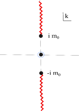
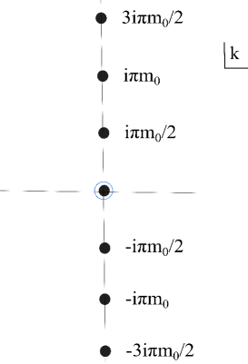
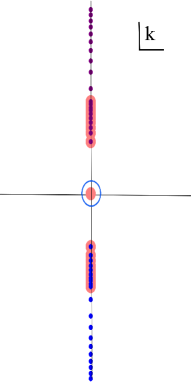
(a) (b) (c)

Figure 3: Singularities governing the two-point function in the complex $k$-plane: (a) of the quantity $G_{q,0}(k)$ for the ground state quench propagator (80), (b) of the quantity $G_{\pm}(k;\beta)$ in the thermal propagator (73), (c) of the quantity $G_{\pm}(k;\beta,\mu_{4})$ in the GGE propagator (77) with $\beta=2,\mu_{4}=0.2$; we have shown 30 leading poles. In each case the pole at the origin is a double pole, and yields the universal linear large distance behaviour of $\langle\phi\,\phi\rangle$. Due to the equivalence between the quenched state and the gCC state (20), the branch cut in (a) can be seen as a limiting case of an accumulation of single poles in a generalized version of (c) with an infinite number of chemical potentials determined by (24), (40). In two-point functions such as $\langle\partial\phi\partial\phi\rangle$, the double poles disappear and the large distance behaviour is sensitive to the sub-leading singularities, which are clearly different. This shows different types of large distance behaviour which are sensitive to the presence of higher dimensional operators.

First look at universality:

Let us first discuss the naive argument for universality in the present context. Note that in case of the sudden quench we found (41)

$$|0,in\rangle=\exp[-\frac{H}{m_{0}}-\frac{5W_{4}}{160m_{0}^{3}}+...]|D\rangle$$

which would appear to imply that, in the limit when the scale of the quench is very high: $m_{0}\to\infty$, the contribution of the Hamiltonian is the most dominant and those of the higher dimensional operators $W_{2n}$, $n>1$, are subdominant. This argument, of course, is flawed, since $m_{0}$ is dimensionful, and the important issue is the relative magnitude of $W_{4}/m_{0}^{3}$ versus $H/m_{0}$ in a particular state.

There are, of course, more refined arguments for universality which define an IR limit in terms of dimensionless distances and times

$$m_{0}r,m_{0}t\gg 1$$ (114)

which is called the deep quench limit in [33]. Ref. [33] argues that in this limit, the propagator in (80) is dominated by the leading expansion of the integrand in $|k|/m_{0}$, which is given by a double pole. From (93), we find that the leading behaviour of this propagator is indeed given by the linear term which is solely determined by this double pole. We find that this double pole and the consequent leading behaviour exactly coincides with that of the thermal propagator (73). Indeed, all three forms of the $\langle\phi\kern 1.0pt\phi\rangle$ propagators, the quenched one (80), the thermal one (73) and the GGE one (77), coincide in the leading behaviour. Thus, the higher order chemical potentials do not modify the leading behaviour. Note, however, that the subleading behaviours are rather different in the three cases: the exponents are different; furthermore, in the quenched propagator there is a prefactor involving a square root.

Lack of Universality:

The long-distance/time leading behaviour of the $\langle\phi\phi\rangle$ propagator is, of course, a rather limited part of the story. Does the above universality hold for correlators involving other operators, in particular, various primary fields (recall that $\phi$ is not a primary field)?

To address this issue, we consider one-point functions of primary fields of the kind $O(z,\bar{z})=\varphi(z)\varphi^{*}(\bar{z})$ which have a decay rate given by (2), (3). For the sudden quench discussed in Section 2.4.1, using (40), we find that the fractional contribution of $W_{2n}$ to the relaxation rate (3) is determined by the dimensionless quantity

$$\tilde{\mu}_{n}=\mu_{n}/\beta^{n-1}\sim\frac{1}{m_{0}^{n-1}}/\left(\frac{1}{m_{0}}\right)^{n-1}$$

which is of order one! What has happened is that, since the quench is characterized by a single scale, the chemical potentials due to the higher dimensional operators are determined by the same mass scale as the temperature, thus the dimensionless contribution due to $W_{n>2}$ is necessarily of order one. In fact, we would expect this kind of behaviour in any single-scale quench (we will make comments about multi-scale quench shortly).

Indeed, we find in (98) that the leading behaviour of the one-point function of $\partial\phi\bar{\partial}\phi$ is not given by the thermal value (nor with any finite number of chemical potentials). This is best understood by looking at the Figure 3. The derivatives $\partial,\bar{\partial}$ kill off the double pole at the origin in all three diagrams, leaving singularities away from the origin. These in Figure (a) differ from those in Figure (b) or in Figure (c). Figure (c), if redone with infinite number of chemical potentials as given by (40), reproduce the singularities of Figure (a).

Thus, we find that all higher dimensional operators are equally important in determining the long time behaviour of this operator. This is also what we anticipated from the MSS expression for the relaxation rate, as explained above.

The same story holds for two-point functions $\langle O(x_{1},t_{1})O(x_{2},t_{2})\rangle$. The exact quench computation, even in the deep quench limit (114) is not reproduced by the thermal result or any finite number of chemical potentials. This can be explicitly seen for $O=\partial\phi$ in the previous two sections. We have also verified this lack of universality for operators which are a composite of ‘derivative’ operators and exponential vertex operators, e.g. $O=\partial\phi e^{iq\phi}$. Once again, the reason is the annihilation of the double pole at the origin by these generic operators.

It is only the pure exponential vertex operators $O=e^{iq\phi}$ whose two-point functions (94) respect universality in the deep quench limit, that is they are reproduced by the thermal behaviour (these operators do not annihilate the pole at the origin).

Multi-scale quench:

The discussion above was mainly centered on a sudden quench from the ground state of a massive theory with mass $m_{0}$. By starting from squeezed states, we can introduce multiple scales in the problem. Thus, as discussed in Section 4.3, it is possible to construct a quantum quench resulting in two parameters $\kappa_{2}$ and $\kappa_{4}$ which are independent (in terms of the asymptotic GGE, the chemical potential $\mu_{4}$ is not determined by $\beta$). The argument about contribution of all higher charges being of the same order, therefore, does not immediately hold. The question then is: suppose we hold $\kappa_{4}$ fixed and small; can we recover thermal behaviour (or, behaviour as in a CC) more or more accurately for sufficiently large times or distances?

To answer this, let us analyze the pole location given by (107)

$$2\kappa_{2}k+2\kappa_{4}k^{3}=i\pi n$$

It would be tempting to argue that for sufficiently small $k$ the cubic term can be ignored to any order of accuracy. However, once we consider correlators which cancel the pole arising from $n=0$, the correlators in Section 4.3 do not receive any contribution at all from small $k$ region. Hence the $\kappa_{4}$ modifies the solution of this equation by $1+o(\kappa_{4}/\kappa_{2}^{3})$ (more precisely, the pole is given by $k_{1}$ from (109) for $n=-1$). Hence the exponent itself changes depending on $\kappa_{4}$, and there is no sense in which the contribution of $\kappa_{4}$ can be made less significant at larger times!

Conclusion:

Generically universality, as defined above, is violated. Long time/distance behaviour is affected by perturbing the initial state by higher dimensional operators. The discussions in this subsection suggest that single scale quenches may generically show such a lack of universality; the same appears to be true of multiple scale quenches where the correlators are dominated by poles at a finite distance from the origin.

5.2 Memory retention

In this section we will discuss the issue of non-standard thermalization in the models studied where the equilibrium chemical potentials allow a reconstruction of the quench protocol (completely or partially depending on the situation).

Quench from a ground state:

Let us first consider the case of quenches from a ground state. As is clear from (13) and (15), the $\kappa_{n}$-coefficients of the gCC state (20) have a one-to-one relation to the reflection amplitude $r(k)$ of the analogous potential scattering problem discussed in Appendix A. Now, it is well-known that the potential of a one-dimensional Schrödinger problem [38, 39, 40] can be reconstructed from the reflection amplitude $r(k)$. As explained above, the potential of the scattering problem is specified by $m(t)$. Hence it follows that $m(t)$ can be reconstructed from $\kappa(k)$. This, in turn, means that the $\mu_{n}$’s, which are just $4\kappa_{n}$ (24) ($\mu_{2}\equiv\beta$), carry complete knowledge of the quench protocol $m(t)$. Thus, the equilibrium ensemble remembers the quench protocol! As an example, the coefficients $\kappa_{n}$ in (34) can be used to determine the parameters $m_{0}$ and $\rho$ which specify the quench protocol $m(t)$ completely.

Quench from excited states:

In case we consider a squeezed pre-quench state, there is additional data in the pre-quench state and the GGE is characterized by the function $\kappa_{\rm eff}(k)$ (53) which is given by a combination of the knowledge of the squeezing function $f(k)$ and the quench protocol $m(t)$ (see (52)). For a known initial state, the quench protocol $m(t)$ can be reconstructed from the GGE parameters $\mu_{n}$ like above. Similarly, for a given quench protocol, the initial state, characterized by $f(k)$ can be completely determined by the $\kappa_{n}$-parameters (see, e.g. (55)). In case the pre-quench initial state as well as the quench protocol are unknown, the GGE allows reconstruction of a certain combination of the data.

One might wonder whether, for a known quench protocol, any initial state can be reconstructed from the final equilibrium ensemble. The answer is no, as can be easily seen by considering a linear combination of several squeezed states. In general, the final equilibrium ensemble has only partial memory of the initial state. Full reconstruction of the initial state happens only for special states like the squeezed states considered in this paper. Of course, besides the choice of the initial state, the integrability of the model is another crucial ingredient for this result. We would comment on the possible holographic interpretation of this result in the next section.

6 Discussion

In this paper, we explicitly verify for actual critical quenches the ansatz made in MSS for the generalized Calabrese-Cardy form (gCC) (1) of the initial state. We show that for an arbitrary mass quench in a theory of free scalars as well as in a theory of free fermions, a large choice of pre-quench initial states (ground state or squeezed states) leads to a gCC state. We find that our results hold even when the quantum quench begins and ends in a massless theory, although in this case, the putative temperature sometimes turns out to be imaginary and the issue of thermalization in these cases is subtle.

We find that while the ground state and generic squeezed states lead to gCC states with all infinite number of $\kappa_{n}$ parameters present, one can choose special squeezed states to prepare gCC states with specific values of any given number of the $\kappa_{n}$-parameters; in particular we can prepare a CC state of the form $e^{-\kappa_{2}H}|D\rangle$ from special squeezed states.

We compute the exact propagator in these quenches and hence the exact time-dependence of correlators. We find that the correlators thermalize at long times and the results verify those of MSS wherever a comparison is possible. We have a simple understanding of the identification (2) of the $\kappa_{n}$’s with the chemical potentials $\mu_{n}$ in terms of poles of the propagator. In specially prepared gCC states with non-zero values of $\kappa_{2}$ and $\kappa_{4}$, we show that the exponential decay given by the relaxation rate (3) persists non-perturbatively in $\kappa_{4}$.

We point out that the presence of the extra charges in the gCC state, which are higher dimensional operators, non-trivially modify the long distance and long time behaviour of correlators, in apparent contradiction to Wilsonian universality. This is an example of a UV/IR mixing; operators which are expected to be relevant in the UV by usual RG arguments are found here to affect the IR behaviour of various correlators. We present an understanding of this in terms of poles of the propagator in the complex momentum plane. We find that while exponential vertex operators do not suffer from these ‘non-universal’ corrections, all other operators (derivatives and composites of derivatives and exponentials) do show this non-universal behaviour.

We also find another atypical behaviour, related to the above: the equilibrium ensemble remembers about the quench protocol. In case we start from the ground state of the pre-quench Hamiltonian, the chemical potentials of the GGE encode a complete knowledge of the quench protocol $m(t)$. With pre-quench squeezed state, the chemical potentials encode a combination of information about the initial state and the quench protocol.

6.1 Higher spin black holes

In MSS [1] we established a relation between (a) relaxation of perturbations to a GGE in a CFT and, in the holographic dual, (b) quasinormal decay to a higher spin (hs) black hole. In particular, we found that the relaxation rate in (a) is equal to the imaginary part of the quasinormal frequency [41] in (b).

We also found in MSS that the rate in (a) is the same as the asymptotic rate of thermalization to a GGE after a quantum quench. This last result depended on an ansatz that the initial state is given by a gCC state. In the present paper we have justified this ansatz; in particular (see, e.g. (56)) we have shown explicitly that a quantum quench from an appropriate squeezed state indeed leads to such gCC states. In Section 4.3 we have shown (see (111)) that the exact formula for the relaxation rate supports the perturbative formula (3). Note that we now have the relaxation rate non-perturbatively, including the two non-perturbative branches (LABEL:poles-exact). It would be interesting to compare these two branches with the corresponding non-perturbative branches of the hs black hole’s quasinormal frequency [41].

The above results prove the relation between quantum quench dynamics in the field theory and quasinormal decay to higher spin black holes. The specific hs black holes relevant to the present paper pertain to the $\lambda\to 1$ and $\lambda\to 0$ limits of the Gaberdiel-Gopakumar correspondence [42] in which the dual conformal field theories describe free massless scalars and free massless fermions respectively. The integrable structure of the conformal field theories is reflected in the infinite number of conserved charges of the hs black hole solutions.

One may wonder if we can extend the above analysis to include gravitational collapse to a hs black hole. Note that a massive to massless quench does not have a direct holographic dual since the theory in the past is not conformal. In this paper we have included a brief discussion of quenches from a critical Hamiltonian to a critical Hamiltonian, starting from ground states/excited states. This can potentially describe a collapse geometry. The relevant CFT calculation indicates that the quench history is determined in a one-to-one fashion by the chemical potentials, or equivalently by the conserved charges. This makes it plausible that in the process of gravitational collapse to a hs black hole, the time-dependent history of the ‘source’ can be reconstructed from the final black hole configuration, in a manner analogous to the dual CFT result on ‘memory retention’ (see subsection 5.2); the parameters specifying the time-dependence are encoded in the infinite number of conserved charges of the black hole.

Other open problems:

Some of the obviously important extensions of the above work are to the case of (i) massive to massive quenches, (ii) higher dimensions, (iii) interacting theories. In particular, it would be interesting if the phenomena of IR non-universality persists in higher dimensions. The calculation of Bogoliubov coefficients and the exact propagator for the tanh protocol appears to go through [28] in higher dimensions in a straightforward manner. However, the analysis of the poles requires more care. We hope to come back to this issue shortly.

Appendix A The analogous scattering problem in quantum mechanics

In the text, we encountered the Klein-Gordon equation (5) expressed in the form

$$-\frac{d^{2}}{dt^{2}}\phi(k,t)+(k^{2}-m^{2}(t))\phi(k,t)=0$$ (115)

We will explain below an analogous Schrödinger problem and inferences for the solution of the above problem.

A.1 Details of the quantum mechanics problem

The equation above is analogous (see Table 2) to the Schrödinger equation for a particle in a potential (we will use the convention $\hbar=1,2m=1$)

$$-\ \frac{d^{2}}{d{\tt x}^{2}}\psi(E,{\tt x})+(V({\tt x})-E)\psi(E,{\tt x})=0$$ (116)

The dictionary is given by

Particle	QFT
${\tt x}$	$t$
$E$	$k^{2}$
$V({\tt x})$	$-m^{2}(t)$
$\psi(E,{\tt x})$	$\phi(k,t)$

Table 2: Analogy

It is understood that $\phi(k,t)$ satisfies the reality condition $\phi^{*}(k,t)=\phi(-k,t)$.

We will first discuss the quantum mechanical scattering problem. For a mass-function $m^{2}(t)$ which drops from $m_{0}^{2}$ to zero, the potential $V({\tt x})$ asymptotes to $-U_{0}\equiv-m_{0}^{2}$ as ${\tt x}\to-\infty$ and to zero as ${\tt x}\to\infty$ (see Figure 4). As is well-known (see, e.g., [43], Section 25), the wavefunction for such a problem takes the asymptotic forms

$$\psi({\tt x}) \xrightarrow{{\tt x}\to-\infty}A_{1}e^{ik_{1}{\tt x}}+B_{1}e^{-ik_{1}{\tt x}},\;k_{1}=\sqrt{(E+U_{0})},$$

$$\xrightarrow{{\tt x}\to\infty}~{}A_{2}e^{ik{\tt x}}+B_{2}e^{-ik{\tt x}},\;k=\sqrt{E}.$$ (117)

The exact solution which matches the above asymptotic form with $A_{2}=1,B_{2}=0$ is called the right-moving Jost function $f_{+}(k,{\tt x})$. There is another exact solution which matches (117) with $B_{1}=1,A_{1}=0$ which is called the left-moving Jost function $\psi(k,{\tt x})=f_{-}(k,{\tt x})$. It can be shown that (for generic momenta) $f_{+}(k,{\tt x})$ and $f_{+}^{*}(k,{\tt x})$ are independent, and so are $f_{-}(k,{\tt x}),f_{-}^{*}(k,{\tt x})$. Clearly $f_{-}$ must be a linear combination of $f_{+},f_{+}^{*}$ and vice versa, expressed in terms of Bogoliubov coefficients $\alpha_{q},\beta_{q}$

$$f_{-}(k,{\tt x})=\alpha_{q}(k)f_{+}(k,{\tt x})+\beta_{q}^{*}(k)f_{+}^{*}(k,{\tt x})$$ (118)

The existence of the Jost functions and properties relevant to the present discussion can be proved under appropriate fall-off conditions of the potential, see, e.g. [39, 40, 38]). In particular a sufficient condition used in [39] is

$$\int_{-\infty}^{\infty}dx\,|V(x)-U_{0}\theta(x)|(1+|x|^{2})<\infty$$ (119)

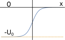
Figure 4: Scattering of a particle in a potential $V({\tt x})$. $V({\tt x})\to-U_{0}$ as ${\tt x}\to-\infty$ and $\to 0$ as ${\tt x}\to\infty$

The general solution of the Schrodinger equation, which has the asymptotic form (117), can be written in two alternative forms

$$\psi(k,{\tt x})=A_{1}(k)f_{-}(k,{\tt x})+B_{1}(k)f^{*}_{-}(k,{\tt x})=A_{2}(k)f_{+}(k,{\tt x})+B_{2}(k)f^{*}_{+}(k,{\tt x})$$ (120)

By using (118) we find the following relations between the $(A_{i},B_{i})$ coefficients (called Bogoliubov relations) [43]:

$$\left(\begin{array}[]{l}A_{2}(k)\\ B_{2}(k)\end{array}\right)=\left(\begin{array}[]{ll}\alpha_{q}&\beta_{q}\\ \beta_{q}^{*}&\alpha_{q}^{*}\end{array}\right)\left(\begin{array}[]{l}A_{1}\\ B_{1}\end{array}\right)$$ (127)

The conservation of particle current along the positive ${\tt x}$-direction implies

$$k_{1}(|A_{1}|^{2}-|B_{1}|^{2})=k(|A_{2}|^{2}-|B_{2}|^{2}),$$ (128)

By applying (127), we get

$$|\alpha_{q}|^{2}-|\beta_{q}|^{2}=k_{1}/k$$ (129)

Let us now consider a wave travelling from the left. This is characterized by $B_{2}=0$ (i.e. as ${\tt x}\to\infty$, $\psi$ becomes purely right-moving). The reflection and transmission amplitudes $r\equiv B_{1}/A_{1}$ and $t\equiv A_{2}/A_{1}$ for such a wave can be easily computed using (127). We get

$$r=-\beta_{q}^{*}/\alpha_{q}^{*},\;t=\alpha_{q}+\beta_{q}B_{1}/A_{1}=\alpha_{q}-|\beta_{q}|^{2}/\alpha_{q}^{*}$$

Note that for a wave of this kind the continuity equation (128) can be rewritten as

$$k_{1}(1-|r|^{2})=k|t|^{2}$$ (130)

Similarly, for a wave travelling from the right, we must have $A_{1}=0$. The corresponding reflection and transmission amplitudes $r^{\prime}=A_{2}/B_{2}$, $t^{\prime}=B_{1}/B_{2}$ can be computed by using (127):

$$r^{\prime}=\beta_{q}/\alpha_{q}^{*},\;t^{\prime}=1/\alpha_{q}^{*}$$ (131)

It is clear that the two reflection amplitudes have the same magnitude:

$$|r^{\prime}|=|r|$$

A.1.1 Power series expansion of the reflection amplitude

It has been shown in [39, 40, 38], under conditions of sufficiently fast fall-off of the potential function at $x=\pm\infty$ ([39] uses (119)) that the right reflection amplitude $r^{\prime}$ has a Taylor expansion around $k=0$, with the leading term $=-1$, thus:

$$r^{\prime}=-1+r_{1}k+r_{2}k^{2}+...,$$ (132)

Below we will demonstrate some explicit examples of such an expansion.

A.1.2 Examples of 1D scattering in QM

1. Consider a step potential $V(x)=-U_{0}\,\Theta(-x)$, with $U_{0}>0$. For such a potential, the asymptotic forms (117) become exact:

   $$\psi({\tt x}) =A_{1}e^{ik_{1}{\tt x}}+B_{1}e^{-ik_{1}{\tt x}},\ {\tt x}<0,\;k_{1}=\sqrt{(E+U_{0})},$$

   $$=A_{2}e^{ik{\tt x}}+B_{2}e^{-ik{\tt x}},\ {\tt x}>0,\;k=\sqrt{E}.$$ (133)

   Demanding continuity of the wavefunction and of its first derivative at $x=0$, we get

   $$\left(\begin{array}[]{l}A_{2}\\ B_{2}\end{array}\right)=\frac{1}{2}\left(\begin{array}[]{ll}1+\frac{k_{1}}{k}&1-\frac{k_{1}}{k}\\ 1-\frac{k_{1}}{k}&1+\frac{k_{1}}{k}\end{array}\right)\left(\begin{array}[]{l}A_{1}\\ B_{1}\end{array}\right)$$

   Using (127) and (131) we can read off the following Bogoliubov coefficients and reflection amplitudes

   $$\alpha_{q}=\frac{1}{2}(1+\frac{k_{1}}{k}),\;\beta_{q}=\frac{1}{2}(1-\frac{k_{1}}{k}),\;r^{\prime}=\frac{\beta}{\alpha^{*}}=\frac{1-\frac{k_{1}}{k}}{1+\frac{k_{1}}{k}},\;r=-\frac{\beta^{*}}{\alpha^{*}}=-\frac{1-\frac{k_{1}}{k}}{1+\frac{k_{1}}{k}},\;k_{1}=\sqrt{k^{2}+U_{0}}$$

   The reflection amplitude $r^{\prime}(k)$ has a Taylor expansion around $k=0$:

   $$r^{\prime}(k)=-1+\frac{2k}{k_{1}}-\frac{2k^{2}}{k_{1}^{2}}+O\left(k^{3}\right)$$

   which has the advertised form (132).

2. Let us consider a piecewise continuous potential

   $$V({\tt x})=\left\{\begin{array}[]{l}-U_{0},\;{\tt x}\leq 0\\ v,\;0<{\tt x}\leq a\\ 0,\;{\tt x}>a\end{array}\right.$$

   where $a>0$ and the constant $v$ can have any real value. The wavefunction has a piecewise form similar to (133), now in three regions (with possibly complex momenta). By demanding continuity of the wavefunction and of its derivative at ${\tt x}=0$ and ${\tt x}=a$, it is straightforward to find

   $$\kern-40.0ptr^{\prime}(k)$$

   $$\kern-50.0pt=\frac{e^{-2iak}\left(\left(k\sqrt{-k^{2}+v}-\sqrt{-\left(k^{2}+U_{0}\right)\left(k^{2}+v\right)}\right)\cosh\left(a\sqrt{-k^{2}+v}\right)+i\left(-k\sqrt{k^{2}+U_{0}}+k^{2}-v\right)\sinh\left(a\sqrt{-k^{2}+v}\right)\right)}{\left(k\sqrt{-k^{2}-U_{0}+v}+\sqrt{-\left(k^{2}+U_{0}\right)\left(k^{2}-v\right)}\right)\cosh\left(a\sqrt{-k^{2}+v}\right)-i\left(k\left(\sqrt{k^{2}+U_{0}}+k\right)-v\right)\sinh\left(a\sqrt{-k^{2}+v}\right)}$$

   $$\kern-50.0pt=-1+k\left[\frac{2\left(-av-i\sqrt{U_{0}}\right)\sinh(a\sqrt{v})+2\left(\sqrt{v}+ia\sqrt{U_{0}v}\right)\cosh(a\sqrt{v})}{\sqrt{U_{0}v}\cosh(a\sqrt{v})+iv\sinh(a\sqrt{v})}\right]+O\left(k^{2}\right).$$

   Note that the Taylor expansion of $r^{\prime}(k)$ in the last line again matches the form (132).

3. For the potential $V({\tt x})=-\frac{1}{2}m_{0}^{2}\left(1-\tanh(\rho{\tt x})\right)$, we find the following Bogoliubov coefficients

   $$\alpha_{q}(k) =\frac{\Gamma\left(-\frac{ik}{\rho}\right)\Gamma\left(1-\frac{ik_{1}}{\rho}\right)}{\Gamma\left(-\frac{i(k+k_{1})}{2\rho}\right)\Gamma\left(1-\frac{i(k+k_{1})}{2\rho}\right)},\quad\beta_{q}(k)=\sqrt{\frac{k}{k_{1}}}\;\frac{\Gamma\left(\frac{-ik}{\rho}\right)\Gamma\left(1-\frac{-ik_{1}}{\rho}\right)}{\Gamma\left(\frac{-i(k-k_{1})}{2\rho}\right)\Gamma\left(1+\frac{-i(k-k_{1})}{2\rho}\right)}\$$

   We can compute these expressions by directly solving the Schrodinger equation; here we have simply borrowed from Section 2.4 and used the dictionary (138). This leads to a reflection amplitude $r^{\prime}(k)=\beta_{q}/\alpha_{q}^{*}$ with the following Taylor series expansion:

   $$r^{\prime}(k)=-1+k\left(-\frac{2}{m_{0}}+\frac{-2i\left(\gamma+\psi^{(0)}\left(-\frac{-im_{0}}{2\rho}\right)\right)}{\rho}\right)+O\left(k^{2}\right)$$

   which, again, agrees with the form (132).

A.2 Implication for the field theory problem

The Klein-Gordon equation for a massive scalar field $\phi(k,t)$ in mixed Fourier space can be written as follows

$$-\ \frac{d^{2}\phi(k,t)}{dt^{2}}=(k^{2}+m^{2})\phi(k,t)$$

The classical solutions are well-known:

$$\phi(k,t)=a(k)\frac{e^{-i\omega(k)t}}{\sqrt{2\omega(k)}}+b(k)\frac{e^{i\omega(k)t}}{\sqrt{2\omega(k)}},\;\omega(k)=+\sqrt{k^{2}+m^{2}}$$

If the scalar field is real, we have $\phi^{*}(k,t)=\phi(-k,t)$, implying $b(k)=a^{*}(-k)$.

In the field theory problem, defined by (115), we have a mass function $m^{2}(t)$ which asymptotes to $m_{0}^{2}$ and zero at $t\to\mp\infty$. In analogy with the Jost function $f_{-}(k,{\tt x})$ introduced above in the analogous Schrödinger problem, we must have an exact solution $\phi(k,t)=u_{in}(k,t)$ which, in the infinite past, asymptotes to

$$u_{in}(k,t)\xrightarrow{t\to-\infty}\frac{e^{-i\omega_{in}t}}{\sqrt{2\omega_{in}}},\;\omega_{in}=\sqrt{k^{2}+m_{0}^{2}}$$

and an exact solution $u_{out}(k,t)$ (analogous to $f_{+}^{*}(k,{\tt x})$) which asymptotes in the far future to

$$u_{out}(k,t)\xrightarrow{t\to\infty}\frac{e^{-i\omega_{out}t}}{\sqrt{2\omega_{out}}},\;\omega_{out}=\sqrt{k^{2}}$$

The normalization of the asymptotic wavefunctions are according to standard conventions. Just like (120), we have two alternative forms of the solution for $\phi(k,t)$:

$$\phi(k,t) =a_{in}(k)u_{in}(k,t)+b_{in}(k)u^{*}_{in}(k,t)=a_{out}(k)u_{out}(k,t)+b_{out}(k)u^{*}_{out}(k,t)$$

$$\xrightarrow{t\to-\infty}\frac{a_{in}}{\sqrt{2\omega_{in}}}e^{-i\omega_{in}t}+\frac{b_{in}}{\sqrt{2\omega_{in}}}e^{i\omega_{in}t}$$

$$\xrightarrow{t\to\infty}\frac{a_{out}}{\sqrt{2\omega_{out}}}e^{-i\omega_{out}t}+\frac{b_{out}}{\sqrt{2\omega_{out}}}e^{i\omega_{out}t}$$ (134)

This can be compared with (117) using Table 2. Further, using the reality properties $b(k)=a^{*}(-k)$ discussed above, we get

$$A_{1}(k)=\frac{a^{*}_{in}(-k)}{\sqrt{2\omega_{in}}},\;B_{1}(k)=\frac{a_{in}(k)}{\sqrt{2\omega_{in}}},\;A_{2}(k)=\frac{a^{*}_{out}(-k)}{\sqrt{2\omega_{out}}},\;B_{2}(k)=\frac{a_{out}(k)}{\sqrt{2\omega_{out}}}$$ (135)

Just like in the quantum mechanics problem, $u_{in}$ is a linear combination of $u_{out}$ and $u^{*}_{out}$ [29]

$$u_{in}(k)=\alpha(k)u_{out}(k)+\beta(k)u^{*}_{out}(-k)$$ (136)

which leads to

$$a_{in}(k)=\alpha^{*}(k)a_{out}(k)+\beta^{*}(k)a^{*}_{out}(-k)$$ (137)

Comparing with (118) and noting the extra normalization factors $1/\sqrt{2\omega}$, we get

$$\alpha(k)=\sqrt{\omega_{out}/\omega_{in}}~{}\alpha_{q}(k),\;\beta(k)=\sqrt{\omega_{out}/\omega_{in}}~{}\beta^{*}_{q}(k)$$ (138)

Here we have used the fact that functions of $\omega$ do not distinguish between $k$ and $-k$.

This proves for us the important relation:

$$\gamma\equiv\beta^{*}/\alpha^{*}=\beta_{q}/\alpha_{q}^{*}=r^{\prime}$$ (139)

Using the above result and (132), we get a Taylor series expansion

$$\gamma=-1+\gamma_{1}k+\gamma_{2}k^{2}+\gamma_{3}k^{3}+...$$ (140)

where the expansion coefficients are the same as in (132), i.e. $\gamma_{i}=r_{i}$.

Another important relation, obtained from (129) and (138) is

$$|\alpha|^{2}-|\beta|^{2}=1$$ (141)

Appendix B Baker-Campbell-Hausdorff Calculation

We will show that

$$|\psi\rangle\equiv\exp\left(\frac{1}{2}\sum_{k}\gamma(k)a^{\dagger}(k)a^{\dagger}(-k)\right)|0\rangle=\exp\left(-\sum_{k}\kappa(k)a^{\dagger}(k)a(k)\right)|Bd\rangle$$ (142)

where

$$\kappa(k)=-\frac{1}{2}\log(\gamma(k)/\gamma_{0})$$ (143)

and

$$|Bd\rangle\equiv\exp\left(\frac{1}{2}\sum_{k}\gamma_{0}a^{\dagger}(k)a^{\dagger}(-k)\right)|0\rangle,$$ (144)

The choice $\gamma_{0}=-1$ corresponds to the Dirichlet state (147) (similarly, $\gamma_{0}=1$ corresponds to Neumann boundary condition). To derive (142), we note that the right hand side can be written as

$$\exp\left[\sum_{k}B(k)\right]\exp\left[\sum_{k}A(k)\right]|0\rangle=\exp\left[\sum_{k}B(k)\right]\exp\left[\sum_{k}A(k)\right]\exp\left[-\sum_{k}B(k)\right]|0\rangle$$

where we have defined $B(k)=-\kappa(k)a^{\dagger}(k)a(k)$ and $A(k)=\gamma_{0}a^{\dagger}(k)a^{\dagger}(-k)$. The identity (142) follows by noting that $[B(l),A(k)]=-\kappa(k)A(k)\left(\delta_{k,l}+\delta_{k,-l}\right)$, and by using the following form of the Baker-Campbell-Hausdorff (BCH) formula

$$e^{X}e^{Y}e^{-X}=e^{\exp(s)Y}$$ (145)

where $[X,Y]=sY$.

In the context of this paper, we will be interested in evaluating $\kappa(k)$ from (143) in a power series in $k$, using (140). Since the leading term in $\gamma(k)$ is $-1$, with the choice of the Dirichlet boundary state $\gamma_{0}=-1$, we get the equation (15) in the text.

Appendix C Bosons

The action for a free massless scalar is

$$S=\frac{1}{2}\int dxdt\left[(\partial_{t}\phi)^{2}-(\partial_{x}\phi)^{2}\right]=-\frac{1}{2}\int dxdt\;\partial_{\mu}\phi\partial^{\mu}\phi$$

The normal mode expansion is (we use “box normalization” $k=2\pi n/L$, $\int\frac{dk}{2\pi}=\frac{1}{L}\sum\limits_{n}$)

$$\phi(x,t) =\int\frac{dk}{2\pi}\left[\frac{a(k)}{\sqrt{2|k|}}\exp\left(ikx-i|k|t\right)+\frac{a^{\dagger}(k)}{\sqrt{2|k|}}\exp\left(-ikx+i|k|t\right)\right]$$

$$=\sum_{n\neq 0}\frac{1}{\sqrt{4\pi L|n|}}a_{n}\exp\left(\frac{2\pi}{L}(inx-i|n|t)\right)+{\rm h.c}$$

$$\equiv\sum_{k\neq 0}\left[\frac{a(k)}{\sqrt{2|k|}}\exp\left(ikx-i|k|t\right)+\frac{a^{\dagger}(k)}{\sqrt{2|k|}}\exp\left(-ikx+i|k|t\right)\right]$$ (146)

We will often use $a_{n}\equiv a(k)$, with a slight abuse of notation. The commutation relations are $[a(k),a^{\dagger}(l)]=\delta_{kl}$.

Boundary states

In terms of standard CFT oscillators $\alpha_{n},\tilde{\alpha}_{n}$, the Dirichlet boundary state is given by (see, e.g. [46] Eq. 4.1.13)

$$|D\rangle=\exp[\sum_{n=1}^{\infty}\frac{1}{n}\alpha_{-n}\tilde{\alpha}_{-n}]|0\rangle$$

In terms of our oscillators $a_{n}\equiv a_{k}$

$$\alpha_{-n}=i\sqrt{n}a^{\dagger}_{-n},\;\tilde{\alpha}_{-n}=i\sqrt{n}a^{\dagger}_{n}$$

$$|D\rangle=\exp[-\sum_{n>0}a^{\dagger}_{n}a^{\dagger}_{-n}]|0\rangle=\exp[-\frac{1}{2}\sum_{n\neq 0}a^{\dagger}_{n}a^{\dagger}_{-n}]|0\rangle=\exp[-\frac{1}{2}\sum_{k\neq 0}a^{\dagger}(k)a^{\dagger}(-k)]|0\rangle$$ (147)

In the first step we used the relation between our oscillators here and the standard CFT conventions (see [45], Chap. 6).

Euclidean CFT

We define $w=x+i\tau$, $\bar{w}=x-i\tau$, $\tau=it$. The Euclidean Propagator is

$$\langle\phi(0,0)\phi(x,\tau)\rangle=\langle\phi(0,0)\phi(w,\bar{w})\rangle=-\frac{1}{4\pi}(\ln w+\ln\bar{w})$$

Vertex operators

Consider the exponential vertex operator $O(w,\bar{w})=\exp[iq\phi(w,\bar{w})]$.

$$\langle\exp[iq\phi(0,0)]\exp[-iq\phi(w,\bar{w})]\rangle=w^{-q^{2}/4\pi}{\bar{w}}^{-q^{2}/4\pi}$$

Hence $h=\bar{h}=q^{2}/8\pi,\;\Delta=q^{2}/4\pi$.

Boson W-currents

We have used the following definitions of the ${\mathbb{W}}_{\infty}$ currents [31] (normal ordering is implicit),

$$T(z) =\partial\phi(z)\partial\phi(z)$$ (148)

$$W_{4}(z) =2\partial^{3}\phi\partial\phi-3\partial^{2}\phi\partial^{2}\phi$$ (149)

Appendix D Fermions

We have used the following conventions in the text.

$$\eta_{\mu\nu}=\begin{bmatrix}1&0\\ 0&-1\end{bmatrix},\quad\partial_{\mu}=(\partial_{t},\partial_{x}),\quad\gamma^{\mu}\partial_{\mu}=\gamma^{0}\partial_{t}-\gamma^{1}\partial_{x},$$

$$\gamma^{0}_{d}=\begin{bmatrix}1&0\\ 0&-1\end{bmatrix},\quad\gamma^{1}_{d}=\begin{bmatrix}0&1\\ -1&0\end{bmatrix},\quad\text{in Dirac basis}.$$

$$S=\frac{1}{\sqrt{2}}\begin{bmatrix}1&-1\\ 1&1\end{bmatrix},\gamma^{0}_{c}=S\gamma^{0}_{d}S^{-1}=\begin{bmatrix}0&1\\ 1&0\end{bmatrix},\quad\gamma^{1}_{c}=S\gamma^{1}_{d}S^{-1}=\begin{bmatrix}0&1\\ -1&0\end{bmatrix},\quad\text{in chiral basis.}$$

$$u(0)=\begin{pmatrix}1\\ 0\end{pmatrix},\qquad v(0)=\begin{pmatrix}0\\ 1\end{pmatrix}\qquad\text{are the spinors in the rest frame.}\$$

The spinors in a general frame are

$$u(k,m) =\frac{1}{\sqrt{(\omega+m)}}\begin{bmatrix}(\omega+m)\\ -k\end{bmatrix}, v(k,m) =\frac{1}{\sqrt{(\omega+m)}}\begin{bmatrix}k\\ -(\omega+m)\end{bmatrix}$$

$$\bar{u}(k,m) =\frac{1}{\sqrt{(\omega+m)}}\begin{bmatrix}(\omega+m)&k\end{bmatrix}, \bar{v}(k,m) =\frac{1}{\sqrt{(\omega+m)}}\begin{bmatrix}k&(\omega+m)\end{bmatrix}$$

where we have used the normalization $\bar{u}(k,m)u(k,m)=-\bar{v}(k,m)v(k,m)=2m$. In the chiral basis, the mode expansion in the massless limit is

$$\Psi_{c}(x,t) = S\cdot\Psi(x,t)=\frac{1}{\sqrt{2}}\begin{bmatrix}1&-1\\ 1&1\end{bmatrix}\cdot\int\frac{dk}{2\pi}\frac{1}{\sqrt{2}}\begin{bmatrix}a_{k}e^{-ik\cdot x}+\text{sgn}(k)b^{\dagger}_{k}e^{ik\cdot x}\\ -\text{sgn}(k)a_{k}e^{-ik\cdot x}-b^{\dagger}_{k}e^{ik\cdot x}\end{bmatrix}$$ (151)

$$= \int_{-\infty}^{\infty}\frac{dk}{2\pi}\frac{1}{2}\begin{bmatrix}(1+\text{sgn}(k))(a_{k}e^{-ik\cdot x}+b^{\dagger}_{k}e^{ik\cdot x})\\ (1-\text{sgn}(k))(a_{k}e^{-ik\cdot x}-b^{\dagger}_{k}e^{ik\cdot x})\end{bmatrix}\$$

Writing as $\psi(x,t)$ and $\bar{\psi}(x,t)$,

$$\psi(x,t) = \int_{0}^{\infty}\frac{dk}{2\pi}(a_{k}e^{-ik\cdot x}+b^{\dagger}_{k}e^{ik\cdot x})$$ (152)

$$\bar{\psi}(x,t) = \int_{-\infty}^{0}\frac{dk}{2\pi}(a_{k}e^{-ik\cdot x}-b^{\dagger}_{k}e^{ik\cdot x})\$$ (153)

Solution of Dirac equation and Bogoliubov coefficients

Using the coordinate transformation $y=e^{-\rho t}$ and the ansatz, we get the following equation:

$$\phi_{\pm}^{\prime\prime}(y)+\frac{\phi_{\pm}^{\prime}(y)}{y}+\phi_{\pm}(y)\left(\frac{k^{2}}{\rho^{2}y^{2}}+\frac{m_{0}^{2}y^{2}\pm 2im_{0}\rho}{\rho^{2}\left(y^{2}+1\right)^{2}}\right)=0$$ (154)

The ‘in’ solutions are solutions which become plane waves in far past and the ‘out’ solutions are solutions which become plane waves in far future. Due to the explicit $i$ in the equation of $\phi_{\pm}$, the positive energy solutions $\phi_{\pm,in/out,p}(k,t)$ and the negative energy solutions $\phi_{\pm,in/out,p}(k,t)^{*}$ are related as

$$\phi_{+,in/out,m}(k,t)=\phi_{-,in/out,p}(k,t)^{*},\qquad\phi_{-,in/out,m}(k,t)=\phi_{+,in/out,p}(k,t)^{*}\$$

So, the solutions can be written as

$$\phi_{+,in/out}(k,t) =\phi_{+,in/out,p}(k,t)+\phi_{-,in/out,p}(k,t)^{*}$$

$$\phi_{-,in/out}(k,t) =\phi_{-,in/out,p}(k,t)+\phi_{+,in/out,p}(k,t)^{*}\$$

The explicit solutions are

$$\phi_{+,in}(k,t) =\left(e^{-2\rho t}+1\right)^{-\frac{im_{0}}{2\rho}}e^{it\left(\omega_{in}+m_{0}\right)}\,_{2}F_{1}\left(\frac{i\left(k-m_{0}-\omega_{in}\right)}{2\rho},\frac{i\left(-k-m_{0}-\omega_{in}\right)}{2\rho};1-\frac{i\omega_{in}}{\rho};e^{2\rho t}\right)$$

$$\phi_{-,in}(k,t) =\left(e^{-2\rho t}+1\right)^{\frac{im_{0}}{2\rho}}e^{-it\left(\omega_{in}-m_{0}\right)}\,_{2}F_{1}\left(\frac{i\left(k+m_{0}-\omega_{in}\right)}{2\rho},\frac{i\left(-k+m_{0}-\omega_{in}\right)}{2\rho};1-\frac{i\omega_{in}}{\rho};e^{2\rho t}\right)$$

$$\phi_{+,out}(k,t) =e^{-ikt}\left(e^{-2\rho t}+1\right)^{-\frac{im_{0}}{2\rho}}\,_{2}F_{1}\left(\frac{i\left(k-m_{0}+\omega_{in}\right)}{2\rho},\frac{i\left(k-m_{0}-\omega_{in}\right)}{2\rho};1+\frac{ik}{\rho};-e^{-2\rho t}\right)$$

$$\phi_{-,out}(k,t) =e^{-ikt}\left(e^{-2\rho t}+1\right)^{\frac{im_{0}}{2\rho}}\,_{2}F_{1}\left(\frac{i\left(k+m_{0}-\omega_{in}\right)}{2\rho},\frac{i\left(k+m_{0}+\omega_{in}\right)}{2\rho};1+\frac{ik}{\rho};-e^{-2\rho t}\right)$$ (155)

Defining the Dirac spinors as

$$U_{in/out}(k,x,t) =K_{in/out}\left(\gamma^{0}\partial_{t}-ik\gamma^{1}-im(t)\right)e^{ikx}\phi_{+,in/out,p}(k,t)u(0)$$

$$V_{in/out}(k,x,t) =-K_{in/out}\left(\gamma^{0}\partial_{t}+ik\gamma^{1}-im(t)\right)e^{-ikx}\phi_{+,in/out,p}(k,t)^{*}v(0)\$$

where $K_{in/out}=i\left(\frac{1}{\omega_{in/out}+m_{in/out}}\right)^{1/2}$. For constant mass, $U(k,x,t)=u(k,m)e^{-ik\cdot x}$ and $V(k,x,t)=v(k,m)e^{ik\cdot x}$ where $u(k,m)$ and $v(k,m)$ have been defined in (LABEL:norspinor). The mode expansion of $\Psi(x,t)$ in terms of in/out modes are

$$\Psi(x,t)=\int_{-\infty}^{\infty}\frac{dk}{\sqrt{2\omega_{in/out}}}\left[a_{k,in/out}U_{in/out}(k,x,t)+b^{\dagger}_{k,in/out}V_{in/out}(k,x,t)\right]\$$

Using properties of hypergeometric functions [34], the Bogoliubov transformations between ‘in’ and ‘out’ solutions are

$$\phi_{+,in,p}(k,t) =\alpha_{+}(k)\phi_{+,out,p}(k,t)+\beta_{+}(k)\phi_{-,out,p}(k,t)^{*}$$

$$\phi_{-,in,p}(k,t) =\alpha_{-}(k)\phi_{-,out,p}(k,t)+\beta_{+}(k)\phi_{+,out,p}(k,t)^{*}\$$

Hence, the Bogoliubov transformations between the ‘in’ and ‘out’ operators are

$$a_{k,in} =\left(\frac{\omega_{in}}{\omega_{out}}\right)^{1/2}\frac{K_{out}}{K_{in}}\left(\alpha_{+}(k)^{*}a_{k,out}-\chi(k)\beta_{+}(k)^{*}b^{\dagger}_{-k,out}\right)$$

$$b_{k,in} =\left(\frac{\omega_{in}}{\omega_{out}}\right)^{1/2}\frac{K_{out}}{K_{in}}\left(\alpha_{+}(k)^{*}b_{k,out}+\tilde{\chi}(k)\beta_{-}(k)^{*}a^{\dagger}_{-k,out}\right)$$ (156)

where $\chi(k)=\tilde{\chi}(k)=\text{sgn}(k)$. It is straightforward now to find the expressions for the Bogoliubov coefficients which are reproduced in the text (67).

Fermion W-currents

We have used the following definitions of the super-${\mathbb{W}}_{\infty}$ currents [47] (normal ordering is implicit),

$$T(z) =-\frac{i}{2}\left(\psi^{*}\partial\psi(z)-\partial\psi^{*}\psi(z)\right)$$

$$W_{4}(z) =\frac{4}{5}q^{2}\left(\partial^{3}\psi^{*}\psi(z)-9\partial^{2}\psi^{*}\partial\psi(z)+9\partial\psi^{*}\partial^{2}\psi(z)-\psi^{*}\partial^{3}\psi(z)\right)$$

Appendix E Subtleties of the sudden limit

In Section 2.4 we analyzed the behaviour of the quench under the “tanh” protocol for large $\rho$ in a power series in $m_{0}/\rho$. In particular, in Section 2.4.1, we defined the sudden limit as the limit (36). In this section we will give a more precise definition of this limit. In certain quantities, like the number operator (35) in Section 2.4 and the propagator in Section 4.2 etc. the distinction is not essential, but in general the naive limit entails UV divergences. E.g. all $W$-charges, including the energy density, under a naive $m_{0}/\rho$ expansion introduced in Section 2.4 appear to have progressively higher UV divergences as one goes down the order. To treat these divergences properly, let us first analyze these. Later on, we will find that terms in this expansion can be resummed to yield finite expressions, provided we define the sudden limit by the equation (158).

The energy density is

$$E/L=\frac{1}{2\pi}\int_{-\Lambda}^{\Lambda}dk|k|N_{k}=m_{0}^{2}\Bigg{(}\frac{1}{8\pi}-\frac{m_{0}^{2}}{32\pi\Lambda^{2}}+O\left(\frac{m_{0}}{\Lambda}\right)^{4}-\frac{m_{0}^{2}}{\rho^{2}}\left[\frac{1}{48}\pi\log\left(\frac{\Lambda}{m_{0}}\right)\right.\\ \left.+\frac{1}{96}\pi\log(4)+\frac{\pi m_{0}^{2}}{192\Lambda^{2}}+O\left(\frac{m_{0}}{\Lambda}\right)^{4}\right]+O\left(\frac{m_{0}}{\rho}\right)^{4}\Bigg{)}$$ (157)

where we have used the asymptotic number density (35), in an $m_{0}/\rho$ expansion:

$$N_{k} =\frac{\left(k-\sqrt{k^{2}+m_{0}^{2}}\right)^{2}}{4k\sqrt{k^{2}+m_{0}^{2}}}-\left(\frac{m_{0}}{\rho}\right)^{2}\frac{\pi^{2}m^{2}_{0}}{48\left(k\sqrt{k^{2}+m^{2}}\right)}+O\left(\frac{m_{0}}{\rho}\right)^{4}$$

The $W_{4}$ density is

$$W_{4}/L =\int_{-\Lambda}^{\Lambda}\frac{dk}{2\pi}|k|^{3}N_{k}=m_{0}^{4}\Bigg{[}\frac{4\log(\Lambda/m_{0})-3+\log(16)}{64\pi}+\frac{m_{0}^{2}}{32\pi\Lambda^{2}}+O\left(\frac{m_{0}}{\Lambda}\right)^{4}$$

$$+\left(\frac{m_{0}}{\rho}\right)^{2}\left(-\frac{\pi\Lambda^{2}}{96m_{0}^{2}}+\frac{1}{192}\pi(2\log(\Lambda/m_{0})-1+\log(4))+\frac{\pi m_{0}^{2}}{256\Lambda^{2}}+O\left(\frac{m_{0}}{\Lambda}\right)^{4}\right)+O\left(\frac{m_{0}}{\rho}\right)^{4}\Bigg{]}$$

The $W_{6}$ density is

$$W_{6}/L=\int_{-\Lambda}^{\Lambda}\frac{dk}{2\pi}|k|^{5}N_{k}= m_{0}^{6}\Bigg{[}\left(\frac{\Lambda^{2}}{32\pi m_{0}^{2}}+\left(\frac{\log\left(\frac{m_{0}}{\Lambda}\right)}{16\pi}+\frac{1}{24\pi}-\frac{\log(4)}{32\pi}\right)-\frac{15m_{0}^{2}}{512\pi\Lambda^{2}}+O\left(\frac{m_{0}}{\Lambda}\right)^{4}\right)+$$

$$\;\qquad+\frac{m_{0}^{2}}{\rho^{2}}\Bigg{(}-\frac{\pi\Lambda^{4}}{192m_{0}^{4}}+\frac{\pi\Lambda^{2}}{192m_{0}^{2}}+\frac{1}{128}\pi\log\left(\frac{m_{0}}{\Lambda}\right)$$

$$\qquad\qquad-\frac{1}{256}\pi\log(4)+\frac{7\pi}{1536}-\frac{5\pi m_{0}^{2}}{1536\Lambda^{2}}+O\left(\frac{m_{0}}{\Lambda}\right)^{4}\Bigg{)}+O\left(\frac{m_{0}}{\rho}\right)^{4}\Bigg{]}$$

E.1 Resumming the divergences

It turns out that the terms with growing UV-divergences with growing powers of $m_{0}/\rho$ can be resummed to the following form.
Introduce the scaling functions

$$E/L=m_{0}^{2}{{\cal E}}(x,y),\quad W_{4}/L=m_{0}^{4}F(x,y),\quad W_{6}/L=m_{0}^{6}G(x,y),\quad x=m_{0}^{2}/\rho^{2},\;y=m_{0}^{2}/\Lambda^{2}$$

The leading singularities in the above expressions for the charges are captured by

$${{\cal E}}(x,y) =\frac{1}{8\pi}+\frac{\left(\frac{5\pi^{2}x}{8}+y\right)\log\left(\pi^{2}x+y\right)}{60\pi}+\cdots=\frac{1}{8\pi}+\cdots$$

$$F(x,y) =-\frac{\left(\log\left(\frac{2\pi^{4}x^{2}}{5}+y^{2}\right)+\log\left(\pi^{2}x+y\right)\right)\left(40\left(5y+3\right)+\pi^{4}x^{2}+20\pi^{2}x\right)}{11520\pi}+\cdots$$

$$G(x,y) =\frac{1}{1536\pi}\left(\frac{\pi^{4}x^{2}}{120}+\frac{1}{32}\pi^{2}x(9y+4)+y^{2}+y+1\right)\left[8\left(\frac{25}{\sqrt{\frac{26\pi^{4}x^{2}}{3}+25y^{2}}}+\frac{1}{\pi^{2}x+y}\right)\right.$$

$$\left.+19\log\left(\frac{74\pi^{4}x^{2}}{285}+y^{2}\right)+10\log\left(\pi^{2}x+y\right)\right]+\cdots$$

The correct version of the “sudden” limit, therefore, is to take the limit $\Lambda\to\infty$ first, for finite, large $\rho/m_{0}$ (see Figure 5), i.e.

$$y=\frac{m_{0}^{2}}{\Lambda^{2}}\to 0,\;x=\frac{m_{0}^{2}}{\rho^{2}}={\rm small,~{}fixed}$$ (158)

In this limit, as we can see from the above expressions:

$${{\cal E}}(x,0)=\frac{1}{8\pi}+\frac{\pi}{96}x\log(x)+\cdots=\frac{1}{8\pi}+\cdots,\quad F(x,0)\propto\log(x)+\cdots,\;G(x,0)\propto\log(x)/x+\cdots,$$

which implies

$$E/L =m_{0}^{2}\left(\frac{1}{8\pi}-\frac{\pi}{48}\frac{m_{0}^{2}}{\rho^{2}}\log(\frac{\rho}{m_{0}})\right)+\cdots=m_{0}^{2}\frac{1}{8\pi}+\cdots$$

$$W_{4}/L \propto m_{0}^{4}\ \log(\frac{\rho}{m_{0}})+\cdots$$

$$W_{6}/L \propto m_{0}^{6}\ \frac{\rho^{2}}{m_{0}^{2}}\log(\frac{\rho}{m_{0}})+\cdots$$ (159)

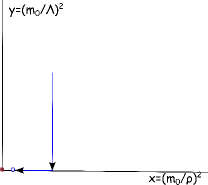
Figure 5: The sudden limit.

References

- [1] G. Mandal, R. Sinha, and N. Sorokhaibam, Thermalization with chemical potentials, and higher spin black holes, JHEP 08 (2015) 013, [arXiv:1501.04580].
- [2] A. Polkovnikov, K. Sengupta, A. Silva, and M. Vengalattore, Nonequilibrium dynamics of closed interacting quantum systems, Rev.Mod.Phys. 83 (2011) 863, [arXiv:1007.5331].
- [3] R. Nandkishore and D. A. Huse, Many body localization and thermalization in quantum statistical mechanics, Ann. Rev. Condensed Matter Phys. 6 (2015) 15–38, [arXiv:1404.0686].
- [4] C. Gogolin and J. Eisert, Equilibration, thermalisation, and the emergence of statistical mechanics in closed quantum systems, tech. rep., arXiv:1503.07538, Mar., 2015.
- [5] S. Bhattacharyya and S. Minwalla, Weak Field Black Hole Formation in Asymptotically AdS Spacetimes, JHEP 0909 (2009) 034, [arXiv:0904.0464].
- [6] P. M. Chesler and L. G. Yaffe, Horizon formation and far-from-equilibrium isotropization in supersymmetric Yang-Mills plasma, Phys. Rev. Lett. 102 (2009) 211601, [arXiv:0812.2053].
- [7] V. Balasubramanian, A. Bernamonti, J. de Boer, N. Copland, B. Craps, et al., Thermalization of Strongly Coupled Field Theories, Phys.Rev.Lett. 106 (2011) 191601, [arXiv:1012.4753].
- [8] S. R. Das, T. Nishioka, and T. Takayanagi, Probe Branes, Time-dependent Couplings and Thermalization in AdS/CFT, JHEP 07 (2010) 071, [arXiv:1005.3348].
- [9] V. Balasubramanian, A. Bernamonti, J. de Boer, N. Copland, B. Craps, E. Keski-Vakkuri, B. Muller, A. Schafer, M. Shigemori, and W. Staessens, Holographic Thermalization, Phys. Rev. D84 (2011) 026010, [arXiv:1103.2683].
- [10] J. Cardy, Quantum Quenches to a Critical Point in One Dimension: some further results, arXiv:1507.07266.
- [11] P. Calabrese and J. Cardy, Time Dependence of Correlation Functions Following a Quantum Quench, Physical Review Letters 96 (Apr., 2006) 136801, [cond-mat/0601225].
- [12] F. H. L. Essler, G. Mussardo, and M. Panfil, Generalized Gibbs Ensembles for Quantum Field Theories, Phys. Rev. A91 (2015), no. 5 051602, [arXiv:1411.5352].
- [13] P. Calabrese, F. H. L. Essler, and M. Fagotti, Quantum quenches in the transverse field Ising chain: II. Stationary state properties, Journal of Statistical Mechanics: Theory and Experiment 7 (July, 2012) 22, [arXiv:1205.2211].
- [14] P. Caputa, G. Mandal, and R. Sinha, Dynamical Entanglement Entropy with Angular Momentum and U(1) Charge, JHEP 1311 (2013) 052, [arXiv:1306.4974].
- [15] T. Barthel and U. Schollwöck, Dephasing and the Steady State in Quantum Many-Particle Systems, Physical Review Letters 100 (Mar., 2008) 100601, [arXiv:0711.4896].
- [16] M. Cramer, C. M. Dawson, J. Eisert, and T. J. Osborne, Exact Relaxation in a Class of Nonequilibrium Quantum Lattice Systems, Physical Review Letters 100 (Jan., 2008) 030602, [cond-mat/0703314].
- [17] M. Rigol, V. Dunjko, V. Yurovsky, and M. Olshanii, Relaxation in a completely integrable many-body quantum system: An Ab Initio study of the dynamics of the highly excited states of 1d lattice hard-core bosons, Phys. Rev. Lett. 98 (Feb, 2007) 050405, [0604476].
- [18] M. Rigol, V. Dunjko, and M. Olshanii, Thermalization and its mechanism for generic isolated quantum systems, Nature 452 (Apr., 2008) 854–858, [arXiv:0708.1324].
- [19] A. Iucci and M. A. Cazalilla, Quantum quench dynamics of the Luttinger model, Physical 80 (2009) 063619, [arXiv:1003.5170].
- [20] D. Fioretto and G. Mussardo, Quantum quenches in integrable field theories, New Journal of Physics 12 (May, 2010) 055015, [arXiv:0911.3345].
- [21] P. Calabrese, F. H. L. Essler, and M. Fagotti, Quantum Quench in the Transverse-Field Ising Chain, Physical Review Letters 106 (June, 2011) 227203, [arXiv:1104.0154].
- [22] P. Calabrese, F. H. L. Essler, and M. Fagotti, Quantum quench in the transverse field Ising chain: I. Time evolution of order parameter correlators, Journal of Statistical Mechanics: Theory and Experiment 7 (July, 2012) 16, [arXiv:1204.3911].
- [23] G. Mandal and T. Morita, Quantum quench in matrix models: Dynamical phase transitions, Selective equilibration and the Generalized Gibbs Ensemble, JHEP 10 (2013) 197, [arXiv:1302.0859].
- [24] B. Bertini, D. Schuricht, and F. H. L. Essler, Quantum quench in the sine-Gordon model, Journal of Statistical Mechanics: Theory and Experiment 10 (Oct., 2014) 35, [arXiv:1405.4813].
- [25] M. Scully and M. Zubairy, Quantum Optics. Cambridge University Press, 1997.
- [26] E. Tiesinga and P. R. Johnson, Collapse and revival dynamics of number-squeezed superfluids of ultracold atoms in optical lattices, Phys. Rev. A 83 (Jun, 2011) 063609.
- [27] S. R. Das, D. A. Galante, and R. C. Myers, Universal scaling in fast quantum quenches in conformal field theories, Phys.Rev.Lett. 112 (2014) 171601, [arXiv:1401.0560].
- [28] S. R. Das, D. A. Galante, and R. C. Myers, Universality in fast quantum quenches, JHEP 1502 (2015) 167, [arXiv:1411.7710].
- [29] N. Birrell and P. Davies, Quantum Fields in Curved Space. Cambridge Monographs on Mathematical Physics. Cambridge University Press, 1984.
- [30] D. Das and S. R. Das, Unpublished, .
- [31] I. Bakas and E. Kiritsis, Bosonic Realization of a Universal Algebra and (infinity) Parafermions, Nucl. Phys. B343 (1990) 185–204. [Erratum: Nucl. Phys.B350,512(1991)].
- [32] S. R. Das, D. A. Galante, and R. C. Myers, Smooth and fast versus instantaneous quenches in quantum field theory, JHEP 08 (2015) 073, [arXiv:1505.05224].
- [33] S. Sotiriadis and J. Cardy, Quantum quench in interacting field theory: A Self-consistent approximation, Phys. Rev. B81 (2010) 134305, [arXiv:1002.0167].
- [34] M. Abramowitz and I. Stegun, Handbook of Mathematical Functions. Dover Publications, 1965.
- [35] A. Perelomov, Generalized Coherent States and Their Applications. Modern Methods of Plant Analysis. Springer-Verlag, 1986.
- [36] A. Duncan, Explicit Dimensional Renormalization of Quantum Field Theory in Curved Space-Time, Phys. Rev. D17 (1978) 964.
- [37] G. Festuccia and H. Liu, The Arrow of time, black holes, and quantum mixing of large N Yang-Mills theories, JHEP 0712 (2007) 027, [hep-th/0611098].
- [38] E. Koelink, Scattering theory, . Lecture notes, Section 4, http://www.math.ru.nl/ koelink/edu/LM-dictaat-scattering.pdf.
- [39] A. Cohen and T. Kappeler, Scattering and inverse scattering for steplike potentials in the schroedinger equation, Indiana Univ. Math. J. 34 (1985) 127–180.
- [40] P. Deift and E. Trubowitz, Inverse scattering on the line, Communications on Pure and Applied Mathematics 32 (1979), no. 2 121–251.
- [41] A. Cabo-Bizet, E. Gava, V. Giraldo-Rivera, and K. Narain, Black Holes in the 3D Higher Spin Theory and Their Quasi Normal Modes, JHEP 1411 (2014) 013, [arXiv:1407.5203].
- [42] M. R. Gaberdiel and R. Gopakumar, An AdS3 Dual for Minimal Model CFTs, Phys.Rev. D83 (2011) 066007, [arXiv:1011.2986].
- [43] L. Landau and E. Lifshitz, Quantum Mechanics: Non-relativistic Theory. Butterworth Heinemann. Butterworth-Heinemann, 1977.
- [44] S. D. Mathur, Is the Polyakov path integral prescription too restrictive?, hep-th/9306090.
- [45] P. Di Francesco, P. Mathieu, and D. Senechal, Conformal field theory, . Springer, New York, USA, 890 p, ISBN: 038794785X.
- [46] B. Craps, D-branes and boundary states in closed string theories. PhD thesis, Leuven U., 2000. hep-th/0004198.
- [47] E. Bergshoeff, C. N. Pope, L. J. Romans, E. Sezgin, and X. Shen, The Super (infinity) Algebra, Phys. Lett. B245 (1990) 447–452.