Bifurcation of lunisolar secular resonances for space debris orbits

Abstract.

Using bifurcation theory, we study the secular resonances induced by the Sun and Moon on space debris orbits around the Earth. In particular, we concentrate on a special class of secular resonances, which depend only on the debris’ orbital inclination. This class is typically subdivided into three distinct types of secular resonances: those occurring at the critical inclination, those corresponding to polar orbits, and a third type resulting from a linear combination of the rates of variation of the argument of perigee and the longitude of the ascending node.

The model describing the dynamics of space debris includes the effects of the geopotential, as well as the Sun’s and Moon’s attractions, and it is defined in terms of suitable action-angle variables. We consider the system averaged over both the mean anomaly of the debris and those of the Sun and Moon. Such multiply-averaged Hamiltonian is used to study the lunisolar resonances which depend just on the inclination.

Borrowing the technique from the theory of bifurcations of Hamiltonian normal forms, we study the birth of periodic orbits and we determine the energy thresholds at which the bifurcations of lunisolar secular resonances take place. This approach gives us physically relevant information on the existence and location of the equilibria, which help us to identify stable and unstable regions in the phase space. Besides their physical interest, the study of inclination dependent resonances offers interesting insights from the dynamical point of view, since it sheds light on different phenomena related to bifurcation theory.

1. Introduction

The gravitational effects of the Sun and Moon in the study of the dynamics of satellites and space debris have recently gained a renewed interest. Indeed, the awareness that a careful investigation of the dynamics of space debris is nowadays mandatory leads to a thorough study of the influence of the Sun and Moon, which are known to provoke important effects in specific regions around the Earth ([43, 16]).

At the present state, one estimates that about $3\times 10^{8}$ objects with size larger than 1 mm and about $3.5\times 10^{5}$ objects larger than 1 cm orbit around the Earth. Leaving all these objects without control could provoke extremely dangerous events. In particular, dramatic scenarios can directly involve operative satellites, or even manned space missions, like the International Space Station. This threat certainly suffices to motivate the efforts which are currently done toward understanding the dynamics of such objects. A mathematical approach to study the dynamics of space debris will strongly depend upon the location of the object one wants to study, since all possible forces (geopotential, atmospheric drag, lunar attraction, solar influences, etc.) contribute to the model in a different way, according to the altitude of the object under investigation.

Adopting the nowadays widespread classification, the circumterrestrial space is divided into following regions:

$\bullet$ LEO (low–Earth orbit), running from 90 to 2 000 km in altitude;

$\bullet$ MEO (medium–Earth orbit), spanning the region between 2 000 and 30 000 km in altitude;

$\bullet$ GEO (geostationary–Earth orbit), used for trajectories around the geosynchronous orbit at altitude of 35 786 km;

$\bullet$ HEO (high–Earth orbit), corresponding to the region above GEO.

In each of the above regions some forces prevail with respect to others. For example, in LEO, beside the gravitational attraction of the Earth, one definitely must consider the effects of the atmospheric drag (thereby dealing with a dissipative dynamical system). In MEO, the gravitational effects of the point–mass Earth and that of the terms corresponding to the second degree and order gravity–field coefficients $J_{2}$ and $J_{22}$ of the spherical harmonics are very important, but also the influence of the Moon and the Sun, including the effect of the solar radiation pressure, become increasingly relevant. Finally, at GEO, as well as in HEO, the lunisolar perturbations become of the same order as the Earth’s oblateness $J_{2}$, and both are more important than the $J_{22}$ (tesseral terms) for long-term orbital dynamics (see [13, 17, 36, 44, 46, 47]). We claim that the model we will introduce in Section 2 is conceived to describe objects in MEO, GEO, HEO, but not in LEO, and therefore it does not include the atmospheric drag.

In this work we concentrate on the effect of lunisolar perturbations ([3, 6, 20]) and precisely on some secular resonances, which depend only on the inclination (see [29], compare also with [30]). With the terms of lunar and solar gravitational resonance we mean that there exists a commensurability relation of the type

$$k_{1}\dot{\omega}+k_{2}\dot{\Omega}+k_{3}\dot{\omega}_{b}+k_{4}\dot{\Omega}_{b}=0$$ (1.1)

for some integers $(k_{1},k_{2},k_{3},k_{4})$, not all identically zero; in (1.1) the quantity $\omega$ denotes the argument of perigee of the debris and $\Omega$ is the longitude of the ascending node, while $\omega_{b}$ and $\Omega_{b}$ are, respectively, the argument of perigee and the longitude of the ascending node of the perturber. When the third–body perturber is the Sun, the suffix will be $b=S$, while it will be $b=M$ for the Moon. As pointed out in [29], taking into account only the secular effects due to $J_{2}$, one can give simple expressions for the rates of variation of $\omega$ and $\Omega$. Inserting such expressions in (1.1) one obtains resonant relations involving the orbital elements $(a,e,i)$ of the debris, where $a$ is the semimajor axis, $e$ the eccentricity and $i$ the inclination. As we will see in Section 3, some of these resonances depend only on the inclination and not on $a$ and $e$ ([29]). The dynamics of such inclination–dependent–only resonances is the object of study of the present work.

To enter the details, one can introduce three main classes of secular resonances depending only on inclination (see Section 3): $(i)$ those corresponding to the so-called critical inclination, $(ii)$ polar orbits, and $(iii)$ the resonances arising from linear combinations of the type $k_{1}\dot{\omega}+k_{2}\dot{\Omega}=0$ with $k_{1}$, $k_{2}\in{\mathbb{Z}}\backslash\{0\}$. The critical inclination is the well-known value $i=63.4^{o}$; polar orbits correspond to $i=90^{o}$; the resonances of type $(iii)$ occur at two specific values of the inclination as given later in (3). These inclinations are referred to the equatorial plane.

A simple, but exhaustive, mathematical model describing the cases $(i)$-$(ii)$-$(iii)$ can be obtained as follows. We introduce the Hamiltonian function including the Keplerian part, the secular part of the geopotential, limited to the most significant term (the so-called $J_{2}$ approximation), and the contributions due to the Moon and the Sun. Following [29, 34, 24], we will conveniently express the elements of the debris with respect to the equatorial plane and those of the Moon with respect to the ecliptic plane; the advantage is that the inclination of the Moon becomes nearly constant and the argument of the perigee of the Moon as well as the longitude of the lunar ascending node vary linearly with time. We refer the reader to [10] for a thorough mathematical derivation of the expansion of the lunisolar Hamiltonian.

We analyze each case (critical inclination, polar case, and linear combination) by properly introducing an adapted system of resonant coordinates; we are thus led to a resonant 2 degrees-of-freedom Hamiltonian that we proceed to average with respect to the fast angle. The action conjugated to the fast angle, say $T$, becomes an integral of motion. Using a technique common in bifurcation theory (see [41, 42, 40]), and which has been successfully applied to the study of the bifurcations of halo orbits around the collinear Lagrangian points ([11]), we investigate the occurrence of bifurcations associated to the lunisolar secular resonances. This leads to an exhaustive study of the generation of families of periodic orbits as the level of the integral $T$, obtained after the averaging process, is varied. We stress that the study of lunisolar resonances is markedly different with respect to the analysis of halo orbits used in [11]. In fact, besides the intrinsic constraints on some dynamical quantities (e.g., positivity of the action variables), the conditions for the existence of bifurcating families of lunisolar resonances include also physical limitations on the orbital elements (most notably the eccentricity) in such a way that their values are compatible with the fact that the perigee of the debris cannot be lower than the Earth’s radius ([5]).

Beside obtaining a physically relevant description of the occurrence of periodic orbits, the results presented in the current work also provide interesting insights into the phenomenon of bifurcations (see also [4, 6]). In particular, we will see that the various types $(i)$-$(ii)$-$(iii)$ of secular resonances must be studied using different variants of the method and that each case leads to a different dynamical behavior. For example, in some cases we need to refine the method and perform very accurate computations to reconstruct the true dynamics, since several bifurcating families coexist (this will be achieved by implementing some expansions to suitable higher orders). Moreover, a connection with the geometric approach to integrable Hamiltonian systems based on their invariants is performed in analogy with the methods used to describe the phenomenon of critical inclination in the most effective way ([14, 15]). This leads to remark that the methods and results presented in this work have a twofold interest: we obtain information on the behavior of lunisolar secular resonances which might be used to study the dynamics of space debris, and we implement bifurcation theory on some case studies, which show different behaviors from the dynamical perspective.

As described before, our study of the bifurcations is based on a multiply averaged system. To understand what happens in the non-averaged model, we provide qualitative arguments: the basic (averaged) model admits whiskered tori and normally hyperbolic invariant manifolds (hereafter, NHIM); the non-averaged system in which the rates of variation of the longitudes of the ascending node of Sun and Moon are assumed to be constant is described by a 2–dimensional Hamiltonian system, for which KAM invariant tori exist, provided that suitable assumptions and non-degeneracy conditions are satisfied; if we consider also the rates of variation of the longitudes of the ascending node of Sun and Moon, then we obtain a non–autonomous, 2–dimensional Hamiltonian model, which might show the phenomenon of Arnold’s diffusion through transition chains between invariant tori. The investigation of such non–averaged models might be the object of study of a future work.

This paper is organized as follows. In Section 2 we introduce a model describing lunisolar secular resonances; in particular, we determine suitable series expansions obtained after a multiple averaging process. Following [29], we compute in Section 3 the secular resonances that depend just on the inclination of the satellite and which lead to the cases $(i)$-$(iii)$ mentioned before. In Section 4 we perform a detailed investigation of the generation of equilibria for the case study $\dot{\omega}+\dot{\Omega}=0$, a sample of class $(iii)$. The analytical study of the resonance $\dot{\omega}+\dot{\Omega}=0$ will be complemented by a numerical investigation through the so-called Fast Lyapunov Indicators (FLIs). The other secular resonances of type $(iii)$ are investigated in Section 5. Secular resonances corresponding to the critical inclination are studied in Section 6 and those corresponding to polar orbits in Section 7. A qualitative description of the dynamics in the non–averaged problem is provided in Section 8. Some conclusions are drawn in Section 9.

2. A model including the lunisolar effect

We consider the motion of a small body, say $D$, that we identify with a space debris. We assume that $D$ is subject to the gravitational influence of the Earth, Sun and Moon. The Hamiltonian describing de dynamics of $D$ has the form (see, e.g., [32, 10, 16]):

$${\mathcal{H}}={\mathcal{H}}_{Kep}+{\mathcal{H}}_{geo}+{\mathcal{H}}_{Moon}+{\mathcal{H}}_{Sun}\ ,$$

where ${\mathcal{H}}_{Kep}$ represents the Keplerian part, ${\mathcal{H}}_{geo}$ describes the perturbation due to the Earth, ${\mathcal{H}}_{Moon}$ and ${\mathcal{H}}_{Sun}$ denote the contributions due to the Moon and Sun, respectively.

We will express the Hamiltonian ${\mathcal{H}}$ in terms of Delaunay action-angle variables, usually denoted as $(L,G,H,M,\omega,\Omega)$, where the actions are defined by

$$L=\sqrt{\mu_{E}a}\ ,\qquad G=L\sqrt{1-e^{2}}\ ,\qquad H=G\cos i$$ (2.1)

with $\mu_{E}={\mathcal{G}}m_{E}$ the product of the gravitational constant ${\mathcal{G}}$ and the mass $m_{E}$ of the Earth, $a$ the semimajor axis, $e$ the orbital eccentricity, $i$ the inclination, while the angle variables are the mean anomaly $M$, the argument of perigee $\omega$, and the longitude of the ascending node $\Omega$.

The quantities $a$, $e$, $i$, $\omega$, $\Omega$ and $M$, called orbital elements, describe the dynamics of $D$. Under the effect of the Keplerian part, all orbital elements, but the mean anomaly $M$ which varies linearly in time, are constant. When a perturbation is considered, the orbital elements are no longer constant, but rather change in time. The long–term variation of the orbital elements can be studied by means of perturbation theory. The first step consists in expanding the perturbation in Fourier series in terms of the orbital elements. The coefficients of the series expansion depend on the semi–major axes, inclinations and eccentricities, while the trigonometric arguments involve linear combinations of the following angles: the mean anomalies, the longitudes of the nodes, the arguments of periapsides. Moreover, the disturbing function depends also on the rotation, hence on the hour angle, of the disturbing body.

Within the infinite number of terms of the series expansion, only some terms are really relevant for the long–term evolution of the orbital elements. In general, the terms of the expansion of the disturbing force are classified as follows: short periodic terms (involving fast angles), secular terms (independent of the fast angles), resonant terms (implying commensurabilities between the fast angles). According to the averaging principle (see, e.g., [38]), the effects of the short periodic terms average out over a long-time. Hence, such terms can be dropped from the expansion and we can focus only on the most relevant terms.

Two types of resonance affect the motion of the space debris (and artificial satellites): $(a)$ tesseral resonances, occurring when there is a commensurability between the Earth’s rotation period and the orbital period of the space debris ([8, 9, 47]), and $(b)$ lunisolar resonances, which involve commensurabilities among the slow frequencies of orbital precession of a satellite and the perturbing body ([29, 30, 20, 10, 16]). Tesseral resonances provoke variations of the semi–major axis on a time scale of the order of hundreds of days, while lunisolar resonances influence the evolution of the eccentricity and inclination on a much longer time scale, of the order of tens (or hundreds) of years. In this work, we focus on the effects induced by the lunisolar resonances. Thus, in the following sections we average the disturbing functions over the mean anomalies of both the space debris and the perturbing bodies.

As it is well known (see, e.g., [7]), the Keplerian part of the Hamiltonian is given by

$${\mathcal{H}}_{Kep}(L)=-{{\mu_{E}^{2}}\over{2L^{2}}}\ .$$

For later convenience, it is important to underline that the units of length and time are normalized so that the geostationary distance is unity (it amounts to $42\,164.1696$ km) and that the period of Earth’s rotation is equal to $2\pi$. As a consequence, from Kepler’s third law it follows that $\mu_{E}=1$. Therefore, unless the units are explicitly specified, the numbers appearing in the following sections will be expressed in the above units.

2.1. The perturbing function ${\mathcal{H}}_{geo}$

As for ${\mathcal{H}}_{geo}$, we limit ourselves to the most important contribution, corresponding to the $J_{2}$ gravity coefficient of the secular part (see, e.g., [8], compare also with [9]), precisely:

$${\mathcal{H}}_{geo}(L,G,H)={{R_{E}^{2}J_{2}\mu_{E}^{4}}\over{4}}\ {{1}\over{L^{3}G^{3}}}\ (1-3{H^{2}\over G^{2}})\ ,$$

where $R_{E}$ is the mean equatorial radius of the Earth and $J_{2}=1.08263\times 10^{-3}$. This expression of the geopotential corresponds to taking an average of the Hamiltonian over the mean anomaly of the space debris as well as over the sidereal time of the Earth, and to consider only the most important term of the expansion in the spherical harmonics of the geopotential.

2.2. The lunar potential

As far as the lunar contribution is concerned, following [34, 24, 29], it is convenient to express the orbital elements of the satellite with reference to the equatorial plane and the orbital elements of the Moon with respect to the ecliptic plane. In fact, since the main perturbing effect is due to the Sun, the motion of the lunar’s elements with respect to the celestial equator, in particular the argument of perigee and the longitude of the ascending node, are such that their changes are nonlinear. For instance, the longitude of the ascending node varies between $-13^{\circ}$ and $+13^{\circ}$ with a period of 18.6 years. On the contrary, if we consider the elements of the Moon with respect to the ecliptic plane, then the inclination $i_{M}$ is close to a constant (in analogy to $a_{M}$ and $e_{M}$), while the variations of the argument of perihelion $\omega_{M}$ and the longitude of the ascending node $\Omega_{M}$ are approximately linear (see for example [45]) with rates $\dot{\omega}_{M}\simeq 0.164^{\circ}/day$, $\dot{\Omega}_{M}\simeq-0.053^{\circ}/day$. The rate of variation of the lunar mean anomaly is $\dot{M}_{M}\simeq 13.06^{\circ}/day$. This implies that the change of $\omega_{M}+\Omega_{M}$ has a period of 8.85 years, while the variation of $\Omega_{M}$ has a period of 18.6 years.

In a first approximation, we assume that the Moon moves on an elliptic orbit with semimajor axis $a_{M}=384\,748/42\,164.1696$ (expressed in units of the geostationary radius), eccentricity $e_{M}=0.0549006$ and inclination $i_{M}=5^{\circ}15^{\prime}$; the mass $m_{M}$ of the Moon, expressed in Earth’s masses, is about equal to 0.0123. The potential due to the lunar attraction will be computed as a truncation of the series expansion to the second order in the ratio of the semi-major axes, so that the lunar potential is approximated by quadrupole fields. Moreover, we will consider the averages of the potential over the mean anomalies of the debris and the Moon (see Section 4). In fact, the mean anomaly of the debris is a fast angle; on the other hand, the mean anomaly of the Moon can be neglected, since the secular resonances we shall consider will not depend upon the mean anomaly of the Moon as well as on that of the Sun (see Remark 2 below).

We proceed now to give an explicit expansion of the lunar potential; to this end, we follow the approach of [34] and [24], recently revisited in [10].

We recall that we denote by $a_{M}$, $\omega_{M}$, $\Omega_{M}$ the semimajor axis, the argument of perigee, the longitude of the ascending node of the Moon referred to the ecliptic plane, respectively. After some computations for which we address the reader to [10], we obtain that ${\mathcal{H}}_{Moon}$ is given by the following expression:

$${\mathcal{H}}_{Moon}=-{\mathcal{R}}_{Moon}\,,$$ (2.2)

where

$${\mathcal{R}}_{Moon} = {1\over 2}\ {\mathcal{G}}m_{M}\sum_{m=0}^{2}\sum_{s=0}^{2}\sum_{p=0}^{2}{a^{2}\over a_{M}^{3}}(-1)^{[{m\over 2}]}\ K_{m}\,K_{s}\ {{(2-s)!}\over{(2+m)!}}$$ (2.3)

$$\ \times F_{2mp}(i)\ F_{2s1}(i_{M})\ H_{2\ p\ 2p-2}(e)\,G_{210}(e_{M})$$

$$\times\Big{\{}U_{2}^{m,-s}\cos\Bigl{(}(2-2p)\omega+m\Omega+s\Omega_{M}-s{\pi\over 2}-y_{s}\pi\Bigr{)}$$

$$+U_{2}^{m,s}\cos\Bigl{(}(2-2p)\omega+m\Omega-s\Omega_{M}+s{\pi\over 2}-y_{s}\pi\Bigr{)}\Big{\}}\ .$$

We consider the expansion up to degree 2 in $a/a_{M}$ and we retain only the terms of the expansion which provide the average over the fast orbital phases (i.e., the mean anomalies of both the debris and the Moon). In (2.3) the following notation has been introduced: $H_{2\ p\ 2p-2}(e)$ and $G_{210}(e_{M})$ are, respectively, the Hansen coefficients $X_{0}^{2,2-2p}(e)$ and $X_{0}^{-3,0}(e_{M})=(1-e_{M})^{-3/2}$ (see [25]); $[\cdot]$ denotes the integer part; $K_{0}=1$, otherwise $K_{m}=2$ if $m\not=0$; $F_{2mp}(i)$ is the Kaula inclination function ([32], see also [12]) that we define for the generic case $F_{nmp}(i)$ as

$$F_{nmp}(i) = \sum_{t=0}^{\min{\{p,[{{n-m}\over 2}]}\}}{{(2n-2t)!}\over{t!(n-t)!(n-m-2t)!\ 2^{2n-2t}}}\sin^{n-m-2t}i\ \sum_{s=0}^{m}\left(\begin{array}[]{c}m\\ s\\ \end{array}\right)\cos^{s}i$$

$$\times\sum_{c}\left(\begin{array}[]{c}n-m-2t+s\\ c\\ \end{array}\right)\left(\begin{array}[]{c}m-s\\ p-t-c\\ \end{array}\right)(-1)^{c-[{{n-m}\over 2}]}\ ,$$

where $c$ is summed over all values for which the binomial coefficients are not zero; the function $U_{2}^{m,s}$ is defined as (compare with [24])

$$U_{2}^{m,s}={{(-1)^{m-s}}\over{(2+s)!}}\ \cos^{s+m}({\varepsilon\over 2})\sin^{s-m}({\varepsilon\over 2})\ {{d^{2+s}}\over{dz^{2+s}}}(z^{2-m}(z-1)^{2+m})\ ,$$

where $z=\cos^{2}({\varepsilon\over 2})$ and $\varepsilon$ denotes the obliquity of the ecliptic, which is equal to $\varepsilon=23^{\circ}26^{\prime}21.45^{\prime\prime}$; the quantity $y_{s}$ is zero for $s$ even and it is equal to $1/2$ for $s$ odd.

2.3. The solar potential

The gravitational potential due to the Sun, ${\mathcal{R}}_{Sun}$, is found analogously to that of the Moon. However, contrary to the lunar case, we use equatorial elements for both the satellite and the Sun (see [31]). Precisely, we assume that the Sun moves on an elliptic orbit with semimajor axis $a_{S}=149\,597\,871/42\,164.1696$ (expressed in units of the geostationary radius), eccentricity $e_{S}=0.01671123$, inclination $i_{S}=23^{\circ}26^{\prime}21.406^{\prime\prime}$, argument of perigee $\omega_{S}=282.94^{\circ}$, longitude of the ascending node $\Omega_{S}=0^{\circ}$; the mass of the Sun $m_{S}$, expressed in Earth’s masses, is equal to about 333 060.4016.

Averaging as in Section 2.2 over the mean anomaly of the space debris and that of the Sun, and truncating to second order in the ratio of semi–major axes, one obtains:

$${\mathcal{H}}_{Sun}=-{\mathcal{R}}_{Sun}\ ,$$ (2.6)

where

$${\mathcal{R}}_{Sun} = {\mathcal{G}}m_{S}\sum_{m=0}^{2}\sum_{p=0}^{2}{a^{2}\over a_{S}^{3}}\ K_{m}\,{{(2-m)!}\over{(2+m)!}}\ F_{2mp}(i)\ F_{2m1}(i_{S})$$ (2.7)

$$\ \times H_{2\ p\ 2p-2}(e)\,G_{210}(e_{S})\ \cos\Bigl{(}(2-2p)\omega+m(\Omega-\Omega_{S})\Bigr{)}\ .$$

The notation appearing in (2.7) has been already introduced in Section 2.2.

We stress that, since in ${\mathcal{H}}_{geo}$, ${\mathcal{H}}_{Moon}$ and ${\mathcal{H}}_{Sun}$ we retain only the secular terms, then it means that we consider the Hamiltonian averaged over $M$ and therefore its conjugated action $L$ turns out to be constant.

3. Secular resonances depending only on inclination

In [29] it has been shown that there are 15 types of third-body (lunar and solar) resonances. This classification accounts for all possible resonances involving a third–body perturber: secular resonances, semi–secular resonances and mean motion resonances.

The semi–secular resonances and mean motion resonances will not be an object of study of the present work: involving the mean anomalies of the Moon and Sun, whose rates of variation are $\dot{M}_{M}\simeq 13^{\circ}/day$, $\dot{M}_{S}\simeq 1^{\circ}/day$, the semi–secular resonances mostly take place in the LEO region. On the other hand, the mean motion resonances occur on a different time scale than the secular resonances. We are indeed interested in gravity secular resonances, which are defined as follows.

Definition 1.

A lunar gravity secular resonance occurs whenever there exists an integer vector $(k_{1},k_{2},k_{3},k_{4})\in{\mathbb{Z}}^{4}\backslash\{0\}$, such that

$$k_{1}\dot{\omega}+k_{2}\dot{\Omega}+k_{3}\dot{\omega}_{M}+k_{4}\dot{\Omega}_{M}=0\ .$$ (3.1)

We have a solar gravity secular resonance whenever there exist $(k_{1},k_{2},k_{3},k_{4})\in{\mathbb{Z}}^{4}\backslash\{0\}$, such that

$$k_{1}\dot{\omega}+k_{2}\dot{\Omega}+k_{3}\dot{\omega}_{S}+k_{4}\dot{\Omega}_{S}=0\ .$$ (3.2)

Remark 2.

The commensurability relations (3.1) and (3.2) are independent on $\dot{M}_{M}$ and $\dot{M}_{S}$; this remark motivated the computations of Section 2, where the expansions ${\mathcal{R}}_{Moon}$ in (2.3) and ${\mathcal{R}}_{Sun}$ in (2.7) have been computed by averaging over $M_{M}$ and $M_{S}$.

We stress that the above definition of secular resonance is as general as possible. However, given the fact that the lunar and solar expansions are truncated to the second order in the ratio of semi–major axes, in view of (2.3) and (2.7), the Hamiltonian ${\mathcal{H}}$ is independent of $\omega_{M}$ and $\omega_{S}$. Therefore, for all resonances studied here, one has $k_{3}=0$. Moreover, since $\dot{\Omega}_{S}\simeq 0$, the relations (3.1) and (3.2) may be rewritten in the particular form:

$$(2-2p)\dot{\omega}+m\dot{\Omega}+\kappa\dot{\Omega}_{M}=0\ ,\qquad m,p=0,1,2,\quad\kappa=-2,-1,0,1,2\,,$$ (3.3)

and

$$(2-2p)\dot{\omega}+m\dot{\Omega}=0\ ,\qquad m,p=0,1,2\,,$$ (3.4)

respectively.

The longitude of the lunar ascending node varies with the rate $\dot{\Omega}_{M}\simeq-0.053^{\circ}/day$, while the quantities $\dot{\omega}$, $\dot{\Omega}$ can be approximated by the following well known formulae, which take into account only the effect of $J_{2}$ ([29]):

$$\dot{\omega} \simeq 4.98\Bigl{(}{R_{E}\over a}\Bigr{)}^{7\over 2}\ (1-e^{2})^{-2}\ (5\cos^{2}i-1)\ ^{\circ}/day\ ,$$

$$\dot{\Omega} \simeq -9.97\Bigl{(}{R_{E}\over a}\Bigr{)}^{7\over 2}\ (1-e^{2})^{-2}\ \cos i\ ^{\circ}/day\ .$$ (3.5)

Inserting (3) in (3.3) or (3.4), we obtain a relation involving the satellite’s elements $a$, $e$, $i$: this expression provides the location of the secular resonance.

As pointed out in [29], some resonances turn out to be independent on $a$, $e$, and they depend only on the inclination. The general class of resonances depending only on the inclination is characterized by the relation $k_{1}\dot{\omega}+k_{2}\dot{\Omega}=0$, $k_{1},k_{2}\in\mathbb{Z}$. From this class, the most important ones are those for which $k_{1},k_{2}\in\{-2,-1,0,1,2\}$. In fact, under the quadrupolar approximation considered in this paper, the only possible resonances are:

$$\dot{\omega} = 0$$

$$\dot{\Omega} = 0$$

$$\dot{\omega}+\dot{\Omega} = 0$$

$$-\dot{\omega}+\dot{\Omega} = 0$$

$$-2\dot{\omega}+\dot{\Omega} = 0$$

$$2\dot{\omega}+\dot{\Omega} = 0\ .$$ (3.6)

The resonances involving $k_{1}$ and $k_{2}$ with $|k_{1}|>2$ or/and $|k_{2}|>2$ occur at higher degree expansions of the lunar and solar disturbing functions, their influence being negligible in the MEO region.

Inserting (3) in (3), one readily sees that one obtains expressions involving just the inclinations. Precisely, the specific values of the inclinations corresponding to the cases listed in (3) are, respectively:

$$63.4^{\circ}\qquad{\rm or}\qquad 116.4^{\circ}$$

$$\qquad\quad\quad 90^{\circ}$$

$$46.4^{\circ}\qquad{\rm or}\qquad 106.9^{\circ}$$

$$73.2^{\circ}\qquad{\rm or}\qquad 133.6^{\circ}$$

$$69.0^{\circ}\qquad{\rm or}\qquad 123.9^{\circ}$$

$$56.1^{\circ}\qquad{\rm or}\qquad 111.0^{\circ}\ .$$ (3.7)

The values in (3) are obtained as follows. Let us consider as an example the third relation in (3) which, together with (3), yields

$$\dot{\omega}+\dot{\Omega}=\Bigl{(}{R_{E}\over a}\Bigr{)}^{7\over 2}\ (1-e^{2})^{-2}\ [4.98(5\cos^{2}i-1)-9.97\cos i]\ ;$$

the last expression is equal to zero for $i=46.4^{\circ}$ and $i=106.9^{\circ}$. In a similar way one finds the other values listed in (3).

According to [29, 44], we consider the following three classes of lunisolar secular resonances depending only on specific values of the inclination:

1. $\dot{\omega}=0$, which occurs at the critical inclinations $i=63.4^{\circ}$, $116.4^{\circ}$;

2. $\dot{\Omega}=0$, which corresponds to polar orbits;

3. $k_{1}\dot{\omega}+k_{2}\dot{\Omega}=0$ for some $k_{1}$, $k_{2}\in\{-2,-1,1,2\}$.

In the following we shall refer to the above cases as secular resonances of types, respectively, $(i)$, $(ii)$, $(iii)$.

The secular resonances appearing in (3) are the most important secular resonances, as their amplitude is larger than the amplitude associated to both the resonances involving the lunar ascending node $\Omega_{M}$ and the resonances of higher order.

Recalling that we averaged over the mean anomalies of the debris and of the third body, we conclude that the Hamiltonian we are going to study (omitting the Keplerian part) has the following form:

$${\mathcal{H}}(G,H,\omega,\Omega,\omega_{M},\Omega_{M},\omega_{S},\Omega_{S}) = {\alpha\over G^{3}}\left(1-3{H^{2}\over G^{2}}\right)-{\mathcal{R}}_{Moon}(G,H,\omega,\Omega,\omega_{M},\Omega_{M})$$ (3.8)

$$- {\mathcal{R}}_{Sun}(G,H,\omega,\Omega,\omega_{S},\Omega_{S})\ ,$$

where, for a given $L=L_{0}$, the quantity $\alpha$ is defined as

$$\alpha\equiv{{R_{E}^{2}J_{2}\mu_{E}^{4}}\over{4L_{0}^{3}}}=6.19325\times 10^{-6}L_{0}^{-3}$$ (3.9)

and $R_{Moon}$, $R_{Sun}$ are given, respectively, in (2.3), (2.7).

4. Secular resonance: $\dot{\omega}+\dot{\Omega}=0$

In this Section, we analyze in detail one of the cases appearing in (3) and precisely we concentrate on the resonance $\dot{\omega}+\dot{\Omega}=0$, which is located at one of the inclinations $i=46.4^{\circ}$ or $i=106.9^{\circ}$. The study of the other resonances in (3) is deferred to Section 5. Under some simplifying assumptions, we introduce a model (see Section 4.1), which is described by an integrable Hamiltonian function. The investigation of periodic orbits is presented in Sections 4.2, 4.3, using two different methods from bifurcation theory. The validity of the model and of the results is analyzed in Section 4.4, through a numerical technique based on the computation of suitable chaos indicators. We remark that the model as well as the computation of periodic orbits through bifurcation theory relies on some series expansions to given orders. The orders used in the current Section for the resonance $\dot{\omega}+\dot{\Omega}=0$ suffice to provide reliable and stable results. However, this might not be the case for other resonances and, in fact, while studying other resonances of type (3) in Section 5, we add a discussion on the accuracy of the expansion of the Hamiltonian model (see Section 5.1).

4.1. The model

We start by introducing resonant variables through the symplectic transformation $(G,H,\omega,\Omega)\rightarrow(S,T,\sigma,\eta)$ defined by

$$\sigma = \omega+\Omega\ ,\qquad\ \ S=G\ ,$$

$$\eta = \Omega\ ,\qquad\qquad\ \ T=H-G\ .$$ (4.1)

From (3.8) we obtain that the resonant Hamiltonian in the variables (4.1) takes the form

$${\mathcal{H}}_{res}(S,T,\sigma,\eta,t) = {\alpha\over S^{3}}\ \Big{(}1-3{{(T+S)^{2}}\over S^{2}}\Big{)}$$ (4.2)

$$- {\mathcal{R}}_{Moon}^{(res)}(S,T,\sigma,\eta,t)-{\mathcal{R}}_{Sun}^{(res)}(S,T,\sigma,\eta,t)\ ,$$

where the dependence on time in (4.2) comes from the linear variations with time of $\Omega_{M}$. The functions ${\mathcal{R}}_{Moon}^{(res)}$, ${\mathcal{R}}_{Sun}^{(res)}$ denote the functions ${\mathcal{R}}_{Moon}$, ${\mathcal{R}}_{Sun}$ in (2.3), (2.7) expressed in terms of the resonant variables introduced in (4.1).

Our goal will be to find energy thresholds at which the bifurcations of lunisolar resonances take place (see Section 4.2). To this end, we need to introduce an integrable Hamiltonian, which is obtained under the following two hypotheses.

H1. Each resonance will be viewed in isolation, not interacting with the other ones.

This means that on the timescale associated to (4.2), we have that $\sigma$ is the resonant (slow) angle, while $\eta$ is a fast angle; therefore, averaging over $\eta$ (i.e., over $\Omega$), we obtain that the contributions due to Moon and Sun are given (in the units specified in Section 2) by the following expressions:

$$\begin{split}&\overline{\mathcal{R}}_{Moon}^{(res)}(S,T,\sigma,t)=0.10142\cdot 10^{-6}a^{2}(2+3e^{2})[-1+3\cos^{2}(i)]\Bigl{[}7.54884-\cos(\Omega_{M})\\ &\qquad+0.00996\cos(2\,\Omega_{M})\Bigr{]}+0.0114\cdot 10^{-6}a^{2}e^{2}[1+\cos(i)]^{2}\Bigl{[}52.2396\cos(2\,\sigma)\\ &\qquad+2.57317\cos(2\,\sigma-2\,\Omega_{M})+23.2372\cos(2\,\sigma-\Omega_{M})-\cos(2\,\sigma+\Omega_{M})\\ &\qquad+0.00476\cos(2\,\sigma+2\,\Omega_{M})\Bigr{]}\,,\end{split}$$ (4.3)

and

$$\begin{split}&\overline{\mathcal{R}}_{Sun}^{(res)}(S,T,\sigma,t)=0.35561\cdot 10^{-6}a^{2}(2+3e^{2})[-1+3\cos^{2}(i)]\\ &\qquad+0.27666\cdot 10^{-6}a^{2}e^{2}[1+\cos(i)]^{2}\cos(2\,\sigma-2\,\Omega_{S})\,,\end{split}$$ (4.4)

where, for a given $L=L_{0}$, we have that $e^{2}=1-S^{2}/L_{0}^{2}$ and $\cos(i)=(T+S)/S$.

H2. We neglect the rates of variation of $\Omega_{M}$ and $\Omega_{S}$.

In fact, we may disregard just the rate of variation of $\Omega_{M}$, since $\dot{\Omega}_{S}$ is indeed very small; as a consequence, we use the following constant values, valid at epoch J2000 ([45]):

$$\Omega_{M}=125.044555^{\circ}\ ,\qquad\Omega_{S}=0^{\circ}\ .$$ (4.5)

Due to the assumption H2, we obtain that the functions $\overline{\mathcal{R}}_{Moon}^{(res)}$, $\overline{\mathcal{R}}_{Sun}^{(res)}$ do not depend anymore on time.

Under the hypotheses H1 and H2, the contribution due to the Moon is given (in the units specified in Section 2) by the following expression:

$$\begin{split}&\overline{R}_{Moon}(S,T,\sigma)=0.82349\cdot 10^{-6}a^{2}(2+3e^{2})[-1+3\cos^{2}(i)]\\ &\qquad+0.4828\cdot 10^{-6}a^{2}e^{2}[1+\cos(i)]^{2}\cos(2\,\sigma-0.42418)\ ,\end{split}$$ (4.6)

while the contribution due to the Sun, say $\overline{R}_{Sun}(S,T,\sigma)$, is expressed by (4.4) with $\Omega_{S}=0$. We are thus led to consider the following reduced model:

$$\overline{R}_{res}(S,T,\sigma)={\alpha\over S^{3}}\ \Big{(}1-3{{(T+S)^{2}}\over S^{2}}\Big{)}-\overline{R}_{Moon}(S,T,\sigma)-\overline{R}_{Sun}(S,T,\sigma)\ .$$

As remarked, e.g., in [20, 43], in many regions of the phase space there can be a delicate interaction between the resonances, leading to a complex secular dynamics. However, the reduced model provided by $\overline{R}_{res}$ leads to an exhaustive description of the bifurcation phenomena. We will discuss in detail in Section 4.4 the assumptions H1 and H2, and we will highlight numerically the differences between the reduced model $\overline{R}_{res}$ and the Hamiltonian (4.2).

After some algebra, one can write the sum of the contributions $\overline{R}_{Moon}$ and $\overline{R}_{Sun}$ as given by the potential $\overline{{\mathcal{R}}}_{MoonSun}$, whose expression is

$$\begin{split}&\overline{R}_{MoonSun}(S,T,\sigma)=1.17909\cdot 10^{-6}a^{2}(2+3e^{2})[-1+3\cos^{2}(i)]\\ &\qquad+0.74373\cdot 10^{-6}a^{2}e^{2}[1+\cos(i)]^{2}\cos(2\,\sigma-0.27047)\ .\end{split}$$ (4.7)

In conclusion, we are led to consider three possible simplified models, which describe only the effect of the Moon, that of the Sun, or both; they are represented by the following Hamiltonians:

$${\mathcal{H}}_{Moon}(S,T,\sigma) = {\alpha\over S^{3}}\ \Big{(}1-3{{(T+S)^{2}}\over S^{2}}\Big{)}-\overline{{\mathcal{R}}}_{Moon}(S,T,\sigma)$$

$${\mathcal{H}}_{Sun}(S,T,\sigma) = {\alpha\over S^{3}}\ \Big{(}1-3{{(T+S)^{2}}\over S^{2}}\Big{)}-\overline{{\mathcal{R}}}_{Sun}(S,T,\sigma)$$

$${\mathcal{H}}_{MoonSun}(S,T,\sigma) = {\alpha\over S^{3}}\ \Big{(}1-3{{(T+S)^{2}}\over S^{2}}\Big{)}-\overline{{\mathcal{R}}}_{MoonSun}(S,T,\sigma)\ ,$$ (4.8)

where $\overline{{\mathcal{R}}}_{Moon}$, $\overline{{\mathcal{R}}}_{Sun}$, $\overline{{\mathcal{R}}}_{MoonSun}$ are given, respectively, in (4.6), (4.4) with $\Omega_{S}=0$, and (4.7).

Our next task is to compute the equilibrium points associated to one of the Hamiltonians (4.1), that we denote generically as ${\mathcal{H}}_{r}$. In particular, we need to find a solution of the equation

$$\dot{S}=-{{\partial{\mathcal{H}}_{r}}\over{\partial\sigma}}=0\ .$$

With reference to (4.1), we can proceed to compute the equilibria for the following models:

1. including just the contribution of the Moon, the equilibria are obtained by solving the equation:

   $$\dot{S}={{\partial\overline{{\mathcal{R}}}_{Moon}}\over{\partial\sigma}}=0\ ,$$

   which leads to $\sigma=0.212$ or $\sigma=1.783$ (modulo $\pi$);

2. including just the contribution of the Sun, the equilibria are obtained by solving the equation:

   $$\dot{S}={{\partial\overline{{\mathcal{R}}}_{Sun}}\over{\partial\sigma}}=0\ ,$$

   which leads to $\sigma=0$ or $\sigma=\pi/2$ (modulo $\pi$);

3. including both contributions of Moon and Sun, the equilibria are obtained by solving the equation:

   $$\dot{S}={{\partial\overline{{\mathcal{R}}}_{MoonSun}}\over{\partial\sigma}}=0\ ,$$

   which admits the solutions $\sigma=0.135$ or $\sigma=1.706$ (modulo $\pi$).

4.2. Birth of periodic orbits

We now want to investigate the birth of periodic orbits for the secular resonance corresponding to the case $\dot{\omega}+\dot{\Omega}=0$. The other resonances appearing in (3) will be analyzed in Section 5.

According to (4.1), we can in principle consider three different cases in which only the Moon is present, only the Sun is taken into account, or rather the joint contribution of the Moon and Sun is considered. However, in the following discussion we shall present the mathematical details related to the more complete case when both the Moon and Sun are considered. The other two cases can be indeed treated in a similar way.

When dealing with the third model in (4.1) with the potential given by (4.7), it is convenient to introduce the angle $s$ such that

$$2s=2\sigma-0.27047\ .$$

Recalling that $T=H-S=S(\cos i-1)$ and using the value $i_{res}=46.4^{\circ}$ at which the resonance occurs, we introduce the quantity

$$S_{0}=\frac{T}{\cos i_{res}-1}=-3.222\,T$$

and we expand the third Hamiltonian in (4.1) around $S_{0}$ up to the second order, thus obtaining:

$${\mathcal{H}}_{exp}(S,T,s;L_{0})={{10^{-6}}\over{L_{0}^{3}T^{5}}}\Big{(}p_{1}(S,T;L_{0})+p_{2}(S,T;L_{0})\cos 2s\Big{)}\ ,$$ (4.9)

where, by using (3.9), $p_{1}$, $p_{2}$ are the following polynomials of degree two in $S$:

$$p_{1}(S,T;L_{0}) = -0.34538T^{2}+16.2362L_{0}^{7}T^{5}+10.6118L_{0}^{5}T^{7}$$

$$+ S^{2}(-0.04081+0.565253L_{0}^{7}T^{3}+7.07456L_{0}^{5}T^{5})$$

$$+ S(-0.26322T+5.99233L_{0}^{7}T^{4}+21.2237L_{0}^{5}T^{6})$$

$$p_{2}(S,T;L_{0}) = L_{0}^{5}T^{3}\Big{(}-0.63474L_{0}^{2}T^{2}+0.743734T^{4}+S^{2}(0.068246L_{0}^{2}+2.97494T^{2})$$

$$+ S(0.68187L_{0}^{2}T+2.97494T^{3})\Big{)}\ .$$

Of course, we could have computed an expansion to higher order, but we will see that in the present case the second order is sufficient to capture the relevant features of the dynamics. We refer to Section 5.1 for the discussion of the accuracy of the expansion to finite order in $S$.

Remark 3.

It is interesting to underline the analogy presented in [6] of the lunisolar secular resonances with the “second fundamental model for second-order resonances” (see [35]); this model was denoted with the acronym SFM2 in [6].

The second fundamental model for first-order resonances, say SFM1, has been introduced in [26]; in this case the resonant Hamiltonian can be reduced to the form

$${\mathcal{H}}_{SFM1}(S,s)=S^{2}+\beta S-2\sqrt{2S}\cos s$$

for some constant $\beta\in{\mathbb{R}}$. On the contrary, the SFM2 describes resonances of second order ([35]) through a Hamiltonian of the form

$${\mathcal{H}}_{SFM2}(S,s)=2S^{2}+\beta S+S\cos 2s$$

(compare with [6]).

As pointed out in [6], some resonances (precisely, those of second-order in the eccentricity) admit more critical points than those described in SFM2. An “extended fundamental model for second order resonances”, say EFM2, can be introduced to describe more general cases through a Hamiltonian function of the form

$${\mathcal{H}}_{EFM2}(S,s)=\gamma S^{3}+2S^{2}+\beta S+S\cos 2s$$

for some constants $\beta,\gamma\in{\mathbb{R}}$.

Recalling that $\sigma$ and $\eta$ are the angle variables conjugated to $S$ and $T$, respectively, the equations of motion associated to (4.9) are given by

$$\dot{S} = {{2\cdot 10^{-6}}\over{L_{0}^{3}T^{5}}}p_{2}(S,T,L_{0})\ \sin 2s$$

$$\dot{s} = {{10^{-6}}\over{L_{0}^{3}T^{5}}}\ \Bigl{(}{{\partial p_{1}}\over{\partial S}}(S,T,L_{0})+{{\partial p_{2}}\over{\partial S}}(S,T,L_{0})\ \cos 2s\Bigr{)}$$

$$\dot{T} = 0$$

$$\dot{\eta} = -{{5\cdot 10^{-6}}\over{L_{0}^{3}T^{6}}}\ \Bigl{(}p_{1}(S,T,L_{0})+p_{2}(S,T,L_{0})\ \cos 2s\Bigr{)}$$ (4.10)

$$+ {{10^{-6}}\over{L_{0}^{3}T^{5}}}\ \Bigl{(}{{\partial p_{1}}\over{\partial T}}(S,T,L_{0})+{{\partial p_{2}}\over{\partial T}}(S,T,L_{0})\ \cos 2s\Bigr{)}\ .$$

The equations (4.2) show that for the Hamiltonian (4.9) the variable $T$ is a constant of motion. Therefore, we are led to investigate a system with only one degree of freedom in the $(s,S)$ phase-plane parametrized by $T$. The essential information is delivered by the fixed points of the reduced flow that can be located by solving the two equations $\dot{S}=0,\dot{s}=0$. The first equation admits the solutions

$$s=0,\pi\ ,\qquad s=\pm{\pi\over 2}\ \ \ \mod 2\pi\ ,$$

or equivalently $\sigma=0.135$, $\sigma=3.277$, $\sigma=1.706$, $\sigma=-1.435$ (modulo $2\pi$). These values will produce pairs of equilibria, which arise from pitchfork bifurcations.

Let us denote by $\dot{s}_{A}$, $\dot{s}_{B}$, the values of $\dot{s}$ at, respectively, $s=0$ and $s={\pi\over 2}$, and let $S_{A}$, $S_{B}$ be the solutions of $\dot{s}_{A}=0$, $\dot{s}_{B}=0$. Using that $L=\sqrt{\mu_{E}a}$ and expanding $S_{A}$, $S_{B}$ in series of $T$ up to the 6th order, one obtains the expressions

$$S_{A} = -3.225\ T+31.712\ a^{7\over 2}\ T^{4}-497.59\ a^{5\over 2}\ T^{6}\ ,$$

$$S_{B} = -3.225\ T+25.789\ a^{7\over 2}\ T^{4}-100.358\ a^{5\over 2}\ T^{6}\ .$$ (4.11)

To determine the bifurcation thresholds according to the technique described, e.g., in [40, 41, 42], we need to constrain the variable $S$ within an interval, which is determined on the basis of the relation of $S$ with the integral of motion represented by $T$. However, in the present situation we have also a physical constraint, which leads to a bound on $S$ on the basis of the following physical considerations (compare with [5, 6]). We know that the maximum value of $S$ could be $S=L$, since the eccentricity must be greater than or equal to zero. On the other hand, from the fact that the distance at perigee cannot be smaller than the radius of the Earth, we obtain a minimum value that $S$ can reach, say $S=S_{min}$. To be explicit, we start from the condition that the distance at perigee should be at least equal to the Earth’s radius:

$$a(1-e)=R_{E}\ ;$$

from this expression we have $e=(a-R_{E})/a$. Taking into account that $e=\sqrt{1-S^{2}/L^{2}}=\sqrt{1-S^{2}/(\mu_{E}a)}$, we obtain

$$1-{S^{2}\over{\mu_{E}a}}={{(a-R_{E})^{2}}\over a^{2}}\ ,$$

whose solution provides (compare with [4]):

$$S_{min}=\sqrt{{(2a-R_{E})\mu_{E}R_{E}}\over{a}}\ .$$ (4.12)

We stress again that such limitation on $S_{min}$ is purely given by physical reasons and that a different choice might lead to other results. From the minimum value of $S$, we obtain the corresponding value for the variable $T$, say $T=T_{0}$, as

$$T_{0}=S_{min}(\cos i_{res}-1)\ ,$$

where $i_{res}$ is the value of the inclination at resonance, as given by (3).

To find explicit expressions of the bifurcation curves in the $(a,T)$-plane of the conserved quantities, we proceed by simplifying as much as possible the necessary algebra. Using a fake parameter $\lambda$, we introduce the following expansions to first order:

$$T_{A}=T_{0}+\lambda\ T_{A1}\ ,\qquad T_{B}=T_{0}+\lambda\ T_{B1}$$ (4.13)

for some unknowns $T_{A1}$, $T_{B1}$. Next, we replace $T_{A}$, $T_{B}$ in the solutions $S_{A}$, $S_{B}$ given by (4.2), respectively, and we expand to first order in $\lambda$ as

$$S_{A}=\tau_{0}^{(A)}(a)+\lambda\ \tau_{1}^{(A)}(a)\ T_{A1}\ ,\qquad S_{B}=\tau_{0}^{(B)}(a)+\lambda\ \tau_{1}^{(B)}(a)\ T_{B1}$$

for some known functions $\tau_{0}^{(A)}$, $\tau_{1}^{(A)}$, $\tau_{0}^{(B)}$, $\tau_{1}^{(B)}$. The quantities $T_{A1}$, $T_{B1}$ are then obtained by solving the equations

$$S_{A}=S_{min}\ ,\qquad S_{B}=S_{min}\ .$$

Finally, we set $\lambda=1$ and we obtain explicit expressions for (4.13). Since they have a quite cumbersome form, we give the series expansions of $T_{A}$, $T_{B}$ around a given semimajor axis, for example that corresponding to the GPS location, namely $a_{GPS}=26\,560/42\,164\simeq 0.6299$:

$$T_{A} = -0.159538-0.0134657\ (a-a_{GPS})+0.039272\ (a-a_{GPS})^{2}\ ,$$

$$T_{B} = -0.159142-0.0120736\ (a-a_{GPS})+0.039572\ (a-a_{GPS})^{2}\ .$$ (4.14)

Figure 1, right panel, shows the plots of the curves $T_{A}$, $T_{B}$ as a function of the semi-major axis for the model including both effects of the Moon and Sun. In a similar way we proceed to determine the bifurcation thresholds just due to the Sun (see Figure 1, middle panel) and those including just the effects of the Moon (see Figure 1, left panel).

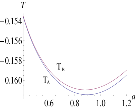
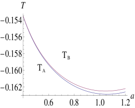
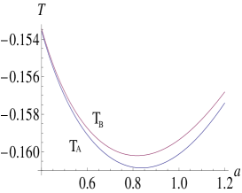
Figure 1. Secular resonance: $\dot{\omega}+\dot{\Omega}=0$, $i=46.4^{o}$. Plots of the bifurcations curves $T_{A}$, $T_{B}$ as a function of the semi-major axis. Left: the Hamiltonian includes just the effect of the Moon; middle: the Hamiltonian includes only the Sun; right: the Hamiltonian includes both Moon and Sun.

The bifurcation values for the GPS orbit are obtained setting $a=a_{GPS}$ in (4.2); in this way we compute the thresholds at which the first and second bifurcations take place (see Table 1).

	inclination (in degrees)		$T_{A}$	$T_{B}$
$\dot{\omega}+\dot{\Omega}=0$	46.4	Moon	-0.159667	-0.159407
$\dot{\omega}+\dot{\Omega}=0$	46.4	Sun	-0.159875	-0.159724
$\dot{\omega}+\dot{\Omega}=0$	46.4	Moon+Sun	-0.159538	-0.159142
$\dot{\omega}+\dot{\Omega}=0$	106.9	Moon	-0.664766	-0.664673
$\dot{\omega}+\dot{\Omega}=0$	106.9	Sun	-0.665209	-0.665155
$\dot{\omega}+\dot{\Omega}=0$	106.9	Moon+Sun	-0.664441	-0.664298

Table 1. Bifurcation values $T_{A}$, $T_{B}$ for the GPS orbit corresponding to the cases in which only the Moon is considered, only the Sun is taken into account, both Sun and Moon are included in the model. The two possible inclinations, $46.4^{o}$ and $106.9^{o}$, found in (3) are considered.

The interpretation of the results is the following. Take a vertical line, for example $a=1$ in Figure 1: below the value $T_{A}$ we do not find any equilibria; for values in the interval $(T_{A},T_{B})$ we have one (hyperbolic) equilibrium point; above $T_{B}$ we find two equilibria (elliptic and hyperbolic). This result is corroborated by Figure 2, which shows the phase space portraits in the plane $(s,S)$ with $s\in[-{\pi},{\pi})$, $S\in[S_{min},S_{max}]$, where $S_{max}=\sqrt{\mu_{E}a}$, corresponding to the GPS value $a=a_{GPS}$. The three panels show the values of $T$ below (left panel), between (middle panel) and above (right panel) the bifurcation thresholds $T_{A}$, $T_{B}$. Given the slight difference between all cases - Sun, Moon, Sun+Moon - as already shown in Table 1, we just provide the results for the sample in which both the Moon and Sun are considered.

We see that Figure 2, left panel, does not exhibit any equilibrium point, while the generation of the two elliptic equilibrium solutions at $s=\pm{\pi\over 2}$ is observed in Figure 2, middle panel, for which the value of $T$ is between those of $T_{A}$ and $T_{B}$ provided in Table 1. For values larger than $T_{B}$ we observe new hyperbolic equilibria at $s=0,\pm\pi$ as shown in Figure 2, right panel.

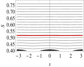
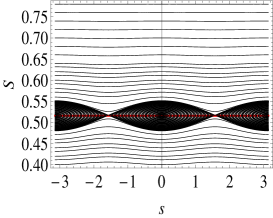
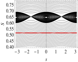
Figure 2. Secular resonance: $\dot{\omega}+\dot{\Omega}=0$, $i=46.4^{o}$. The red line corresponds to the value $S=S_{min}$. Phase space portraits corresponding to the GPS value $a=a_{GPS}$ in the plane $(s,S)$ for the Hamiltonian including both the Moon and Sun: $T=-0.12$ (left), $T=-0.1595$ (middle), $T=-0.2$ (right).

4.3. An alternative method for detecting bifurcations

An alternative method to find bifurcations with respect to the technique presented in Section 4.2 relies on the following procedure, which is based on the geometric approach used in [41, 42] and is related to the analysis of the critical inclination in [14].

Let us come back to the Hamiltonian (4.9). We introduce Poincaré variables defined as

$$x_{1} = L_{0}e\cos s$$

$$x_{2} = L_{0}e\sin s\ ,$$ (4.15)

and we notice that

$$x_{1}^{2}-x_{2}^{2}=L_{0}^{2}e^{2}\cos 2s\ .$$

Then, we can write (4.9) as

$${\mathcal{H}}_{exp}(x_{1},x_{2},T;L_{0})=H_{1}(S,T;L_{0})+H_{2}(S,T;L_{0})\ (x_{1}^{2}-x_{2}^{2})$$ (4.16)

for suitable functions $H_{1}=H_{1}(S,T;L_{0})$, $H_{2}=H_{2}(S,T;L_{0})$. Due to the properties of the angular momentum and of the Laplace-Runge-Lenz vector (see [14]), the variables (4.3) satisfy the identity

$$x_{1}^{2}+x_{2}^{2}+S^{2}=L_{0}^{2}\ ,$$ (4.17)

which defines a reduced phase space. Let us then introduce the variables

$$X = x_{1}^{2}-x_{2}^{2}$$

$$Y = 2x_{1}x_{2}$$

$$Z = S\ ,$$

such that (4.17) becomes

$$X^{2}+Y^{2}=(L_{0}^{2}-S^{2})^{2}\ .$$ (4.18)

We observe that (4.16), expressed in these new variables, depends on $X$, $Z$ but not on $Y$, so that its level surfaces are parabolic cylinders intersecting the lemon-shaped surface (4.18) on curves symmetric with respect to the inversion $Y\rightarrow-Y$. Therefore, all information about the bifurcation of periodic orbits and the birth of equilibria can be inferred by investigating the mutual positions of the boundary set of the lemon

$${\mathcal{L}}\equiv\{(X,Z)\in{\mathbb{R}}^{2}\ :\ \ X=\pm(L^{2}-Z^{2})\}\ ,$$

and the family of curves, parametrized by the level set $h$ of the Hamiltonian, as

$$\{(Z,X(Z))\in{\mathbb{R}}^{2}\ :\ \ {\mathcal{H}}_{exp}(Z,T;L_{0})=h\}\ .$$

From (4.16) we can express the coordinate $X$ as

$$X(Z,T;L_{0},h)={{h-H_{1}(Z,T;L_{0})}\over{H_{2}(Z,T;L_{0})}}\ .$$

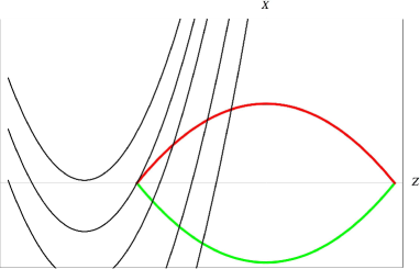
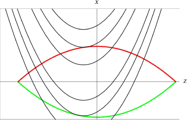
Figure 3. The tangency between the reduced phase space and the energy surface provides the bifurcation of the equilibria.

The equilibrium points are found by imposing the tangency between the boundary of the reduced phase space ${\mathcal{L}}$ and the function $X=X(Z,T;L_{0},h)$ for a given energy level ${\mathcal{H}}_{exp}=h$ that is well approximated by a family of parabolae, sliding parallel to the $Z$-axis by varying the energy value $h$ and parallel to the $X$-axis by varying the value of the second integral $T$. The left panel in Figure 3 shows the case with no contacts when $T<T_{A},T_{B}$. When both thresholds are passed (right panel), the first contact point with the upper branch of the lemon provides the first bifurcation (stable, because it is an external contact, see [42]), while the last contact point yields the second bifurcation (unstable, being an internal contact). The intermediate case is easily guessed as the case in which the vertex of the parabola remains to the left of the corner of the lemon.

Making explicit computations to determine the first and second thresholds one obtains the same results as in Table 1.

4.4. A cartographic study of the resonance $\dot{\omega}+\dot{\Omega}=0$ by using the FLIs

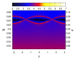
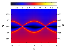
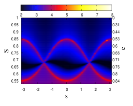
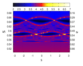
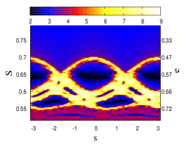
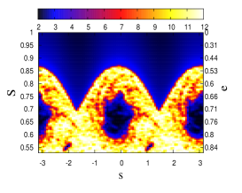
Figure 4. FLI map for the secular resonance $\dot{\omega}+\dot{\Omega}=0$ with $T=-0.2$, and $a=20\,000\,km$ (left panels), $a=26\,560\,km$ (center panels), $a=42\,164\,km$ (right panels). Top panels correspond to the RM2 model, while bottom panels are computed for the RM1 model. The total time span is 465 years (equal to $25\cdot 18.6$ years).

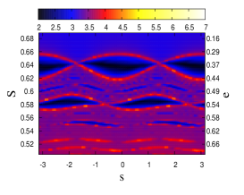
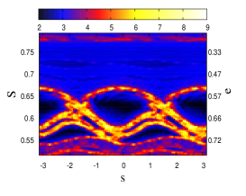
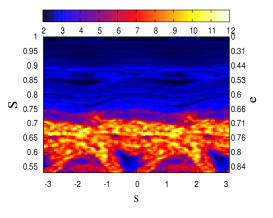
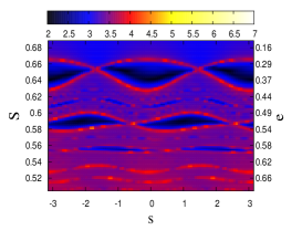
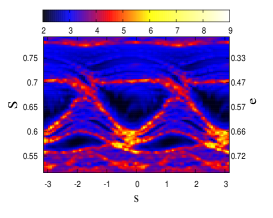
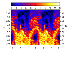
Figure 5. FLI map for the secular resonance $\dot{\omega}+\dot{\Omega}=0$ with $T=-0.2$ and $a=20\,000\,km$ (left panels), $a=26\,560\,km$ (center panels), $a=42\,164\,km$ (right panes). The initial $\Omega$ in the top panels is $\Omega=0^{o}$, while the bottom panels are obtained for $\Omega=180^{o}$. The panels correspond to the DAH model. The total time span is 465 years (equal to $25\cdot 18.6$ years).

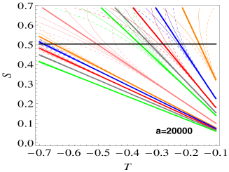
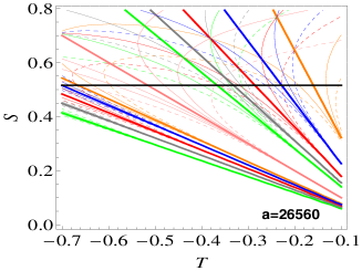
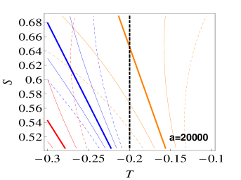
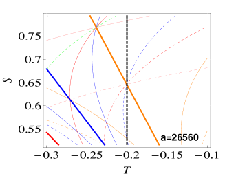
Figure 6. The web structure of lunisolar resonances in the space of the actions for $a=20\,000$ km (left panels) and $a=26\,560$ km (right panels). The thick curves represent the location of the resonances depending only on inclination ($k_{4}$=0 in (3.1) and (3.2), or $\kappa=0$ in (3.3)): $\dot{\Omega}=0$ (pink color, $i=90^{\circ}$), $\dot{\omega}-\dot{\Omega}=0$ (green color, $i=73.2^{\circ}$, $i=133.6^{\circ}$), $2\dot{\omega}-\dot{\Omega}=0$ (grey color, $i=69.0^{\circ}$), $i=123.9^{\circ}$, $\dot{\omega}=0$ (red color, $i=63.4^{\circ}$, $i=116.6^{\circ}$), $2\dot{\omega}+\dot{\Omega}=0$ (blue color, $i=56.1^{\circ}$, $i=111^{\circ}$) and $\dot{\omega}+\dot{\Omega}=0$ (orange color, $i=46.4^{\circ}$, $i=106.9^{\circ}$). The thin curves give the position of the resonances $(2-2p)\dot{\omega}+m\dot{\Omega}+\kappa\dot{\Omega}_{M}=0$ with $p,m\in\{0,1,2\}$, and $\kappa\in\{-2,2\}$ (dashed lines) or $\kappa\in\{-1,1\}$ (continuous lines). The horizontal black lines (top panels) are obtained for $S=S_{min}$, while the vertical black dashed lines (bottom panels) correspond to the value of $T$ used in computing the Figures 2 (right panel), 4 and 5. Top panels are obtained for $S\in[0,S_{max}]$, whereas in the bottom plots $S$ varies from $S_{min}$ to $S_{max}$, as explained in the text.

The reduced model studied in Section 4 is derived under the assumptions H1 and H2, which express that the resonance $\dot{\omega}+\dot{\Omega}=0$ is isolated (namely, it does not interact with the other resonances and therefore the Hamiltonian may be averaged over the fast angle $\eta$) and that $\Omega_{M}$ is constant. The purpose of this Section is to discuss in detail these assumptions and to test whether the reduced model provides reliable results on the bifurcations of periodic orbits. To this end, we consider three models to which we refer as DAH, RM1 and RM2, where:

a) DAH is the full model based on the doubly–averaged Hamiltonian (4.2). We underline that this model provides satisfactory results when compared with higher–fidelity models, which consider higher order terms in the lunisolar perturbations as well as in the geopotential (compare also with [16]);

b) RM1 is the reduced model characterized by the Hamiltonian (4.2) averaged also over $\eta$ (namely, it takes into account the effects of $J_{2}$, $\overline{\mathcal{R}}_{Moon}^{(res)}$ and $\overline{\mathcal{R}}_{Sun}^{(res)}$, where the contributions due to the Moon and Sun are given by (4.3) and (4.4));

c) RM2 is described by the third Hamiltonian in (4.1).

In order to compare these models, we compute the Fast Lyapunov Indicators, hereafter FLIs ([23]), which are suitable chaos indicators allowing us to find the equilibrium points and to distinguish between resonant, stable and chaotic motions. Figures 4 and 5 show the FLI values in the $(s,S)$ plane, where $s\in[-\pi,\pi]$, $S\in[S_{min},S_{max}]$, for $T=-0.2$ and for $a=20\,000\,km$ (left panels), $a=26\,560\,km$ (middle panels) and $a=42\,164\,km$ (right panels). Figure 4 presents the results obtained for the models RM2 and RM1, while Figure 5 shows the FLI values for the DAH model.

Moreover, in order to offer an analytical background for the numerical results depicted in Figures  4 and 5, we show in Figure 6 the structure of lunisolar resonances in the space of the actions $(T,S)$, for $a=20\,000\,km$ (left panels) and $a=26\,560\,km$ (right panels). The analytical estimate of the location of each resonance defined by the relation (3.3) is obtained by approximating $\dot{\omega}$ and $\dot{\Omega}$ with the expressions (3) which consider only the effect of $J_{2}$. We avoid presenting similar plots for $a=42\,164\,km$, because in the GEO region the secular effects of the Moon and Sun are comparable to those of $J_{2}$.

Before describing in detail the results shown in Figures 4 and 5, let us discuss first the meaning of Figure 6. The colored curves provide the location of each resonance; thick lines are associated to the inclination–dependent–only lunisolar resonances $(2-2p)\dot{\omega}+m\dot{\Omega}=0$, $p,m=0,1,2$, while the thin curves give the position of the resonances $(2-2p)\dot{\omega}+m\dot{\Omega}+\kappa\dot{\Omega}_{M}=0$, with $p,m\in\{0,1,2\}$, and $\kappa\in\{-1,1\}$ (continuous curves) or $\kappa\in\{-1,1\}$ (dashed curves). Upper panels show the resonant structures for $S\in[0,S_{max}]$. These plots contain also the horizontal black line $S=S_{min}$, where $S_{min}$ is computed from the condition that the distance of the perigee cannot be smaller than the radius of the Earth (see the relation (4.12)). Therefore, the interval of interest is $[S_{min},S_{max}]$ and the bottom panels of Figure 6 magnify the region associated to the orbits that do not collide with the Earth, at least within a small interval time. The vertical black dashed lines correspond to the value $T=-0.2$, used in computing the FLI maps.

Let us return now to Figures 4 and 5. We stress that besides the values of $S$, displayed on the vertical axis (on the left), in each plot we show the eccentricity values (on the right), computed by using the relations (2.1) and (4.1). Since $T$ is fixed, in a similar way we may compute and display the inclination values.

From (4.7) it follows that the RM2 model used to investigate the bifurcations admits just a single resonant term, and the corresponding phase space is similar to a pendulum (see Figure 4, top panels).

Taking into account the variation of $\Omega_{M}$, namely if we consider the model RM1, then from (4.3) it is evident that the resonant part contains multiple terms, whose arguments are of the form $2\,\sigma\pm\kappa\,\Omega_{M}$ with $\kappa=1,2$. In analogy to the case of the so-called minor resonances for space debris ([9]), we may say that the secular resonance $\dot{\omega}+\dot{\Omega}=0$ splits into a multiplet of resonances, which leads to the phenomenon of splitting or overlapping of resonances (compare also with [20, 43]). These phenomena are clearly explained in [9], but in the framework of tesseral resonances.

From (4.3) it turns out that the two resonant terms with arguments $2\,\sigma$ and $2\,\sigma-\,\Omega_{M}$ are much larger in magnitude than the others. As a consequence, it is reasonable to expect that the islands associated to $2\,\sigma$ and $2\,\sigma-\,\Omega_{M}$ are much larger than the islands associated to the other resonant terms. This aspect is evident from Figure 4, bottom left panel, which shows two larger islands having the centers approximately at $S=0.64$ (corresponding to $2\,\sigma$) and at $S=0.58$ (associated to $2\,\sigma-\,\Omega_{M}$). A smaller island, corresponding to $2\,\sigma-\,2\Omega_{M}$ is located approximately at $S=0.55$. In fact, the bottom left panel of Figure 6 provides an analytical argument for the existence of these islands; the vertical dashed black line $T=-0.2$ intersects three orange curves, corresponding to the following resonances: $\dot{\sigma}=0$ (the thick line), $2\dot{\sigma}-\dot{\Omega}_{M}=0$ (the continuous curve) and $\dot{\sigma}-\dot{\Omega}_{M}=0$ (the dashed curve). As a conclusion, we may say that the bottom left panel of Figure 4, obtained for $a=20\,000\,km$, shows a splitting phenomenon, since the resonant islands are clearly separated. For larger semimajor axis, that is $a=26\,560\,km$, the resonant islands are not so clearly separated as shown in Figure 4, bottom middle panel, or they completely overlap for $a=42\,164\,km$ as in Figure 4, bottom right panel.

Finally, in Figure 5 we give the FLI values obtained by using the non–autonomous two degrees of freedom Hamiltonian (4.2). The top panels show the results obtained for $\Omega=0^{\circ}$, while the bottom panels present the results for $\Omega=180^{\circ}$. For $a=20\,000\,km$ the bottom left panel of Figure 4 and the left plots of Figure 5 are almost identical, thus showing that the average over $\eta$ provides a reliable model: the resonance $\dot{\omega}+\dot{\Omega}=0$ is isolated from the other resonances and $\eta$ (i.e., $\Omega$) is a fast angle. For $a=26\,560\,km$ the bottom middle panel of Figure 4 and the middle plots of Figure 5 show some small differences as effect of both the variation of $\Omega$ and the interaction between various resonances (see the bottom right panel of Figure 6). Despite these differences, the patterns shown by these plots are very similar in structure, suggesting that, with a certain degree of approximation, the RM1 model provides reliable results. For a larger semimajor axis, that is for $a=42\,164\,km$, $\Omega$ is slower than in the case of the MEO region; therefore, a marked difference is visible when comparing the bottom right panel of Figure 4 and the right plots of Figure 5.

The analysis of Figures 4 and 5 show that the model RM2, used to study the bifurcations, yields reliable results for the dynamics related to the bigger island, provided that the main resonant island does not interact with possibly existing smaller islands. As far as the secular resonance $\dot{\omega}+\dot{\Omega}=0$ is concerned, we have a good performance of the model RM2, especially for not too large values of the semimajor axis. Indeed, the equivalent of Figure 2, right panel, but computed for $a=20\,000$ km, overlaps almost completely with the bigger (upper) islands shown in Figures 4 and 5, left panels. Another consequence of the comparison of the panels of Figures 4 and 5 is that a non-zero rate of variation of $\Omega_{M}$ provokes substantial changes in the plots given by RM2 and RM1. This remark is in agreement with the results found in [43].

In conclusion, Figures 4 and 5 show that the long–term dynamics of space debris is very complicated and it is influenced by various effects. However, without a study of the simplest models introduced in Section 4.1, the real dynamics would be difficult to explain.

5. Bifurcations of other secular resonances of type (3)

In Section 4 we have shown the details for the computation of the bifurcation thresholds for the resonance $\dot{\omega}+\dot{\Omega}=0$. The other three resonances appearing in (3) can be treated in a similar way and are analyzed in this Section.

We premise that, whereas the case corresponding to $-\dot{\omega}+\dot{\Omega}=0$ is a straightforward generalization of the case $\dot{\omega}+\dot{\Omega}=0$ in the SFM2 class (see Remark 3 for the definition of the SFM2), the $\pm 2\dot{\omega}+\dot{\Omega}=0$ cases belong to the so-called extended fundamental model for second–order resonances, denoted as EFM2 in Remark 3 (see [35, 6]). The cases corresponding to EFM2 are characterized by the appearance of an additional critical point in the reduced problem corresponding to a new family of periodic orbits of the system.

For the resonance $-\dot{\omega}+\dot{\Omega}=0$, one needs to make the symplectic transformation of coordinates

$$\sigma = \omega-\Omega\ ,\qquad\ \ S=G\ ,$$

$$\eta = \Omega\ ,\qquad\qquad\ \ T=H+G\ .$$

For the resonance $-2\dot{\omega}+\dot{\Omega}=0$, one can make the change of coordinates:

$$\sigma = 2\omega-\Omega\ ,\qquad S={G\over 2}\ ,$$

$$\eta = \Omega\ ,\qquad\qquad\ \ T=H+{G\over 2}\ .$$

For the resonance $2\dot{\omega}+\dot{\Omega}=0$, one makes the transformation of variables:

$$\sigma = 2\omega+\Omega\ ,\qquad S={G\over 2}\ ,$$

$$\eta = \Omega\ ,\qquad\qquad\ \ T=H-{G\over 2}\ .$$

The resonance $-\dot{\omega}+\dot{\Omega}=0$ can be treated in a way similar to that of Section 4; the same holds for the resonances $2\dot{\omega}+\dot{\Omega}=0$ and $-2\dot{\omega}+\dot{\Omega}=0$, when the inclination is equal to $111.0^{\circ}$ and $69.0^{\circ}$, respectively. One has two exceptions: $2\dot{\omega}+\dot{\Omega}=0$ at inclination $56.1^{\circ}$ and $-2\dot{\omega}+\dot{\Omega}=0$ at inclination $i=123.9^{\circ}$. In fact, since $H=S\cos i$, we find in the first case that $T=S(\cos i-{1\over 2})$, which is close to zero when $i=56.1^{\circ}$. As a consequence, since the expansion of the Hamiltonian (compare with (4.9)) contains $T$ at the denominator, the method presented in Section 4.2 fails. The same happens for the latter case.

It could be that different techniques (e.g., other changes of coordinates regularizing the problem) are successful, but the analysis of this problem goes beyond the aims of the present work.

For the moment we limit ourselves to consider the other non-singular cases for which the results are provided in Table 2.

	inclination (in degrees)		$T_{A}$	$T_{B}$
$-\dot{\omega}+\dot{\Omega}=0$	73.2	Moon	0.664659	0.664754
$-\dot{\omega}+\dot{\Omega}=0$	73.2	Sun	0.665149	0.665204
$-\dot{\omega}+\dot{\Omega}=0$	73.2	Moon+Sun	0.664278	0.664423
$-\dot{\omega}+\dot{\Omega}=0$	133.6	Moon	0.159407	0.159667
$-\dot{\omega}+\dot{\Omega}=0$	133.6	Sun	0.159724	0.159875
$-\dot{\omega}+\dot{\Omega}=0$	133.6	Moon+Sun	0.159142	0.159538
$-2\dot{\omega}+\dot{\Omega}=0$	69.0	Moon	0.442037	0.442172
$-2\dot{\omega}+\dot{\Omega}=0$	69.0	Sun	0.442480	0.442546
$-2\dot{\omega}+\dot{\Omega}=0$	69.0	Moon+Sun	0.441693	0.441897
$2\dot{\omega}+\dot{\Omega}=0$	111.0	Moon	-0.442172	-0.442037
$2\dot{\omega}+\dot{\Omega}=0$	111.0	Sun	-0.442546	-0.44248
$2\dot{\omega}+\dot{\Omega}=0$	111.0	Moon+Sun	-0.441897	-0.441693

Table 2. Bifurcation values $T_{A}$, $T_{B}$ for the GPS orbit corresponding to the cases in which only the Moon is considered, only the Sun is considered, both Sun and Moon are considered. The resonances were listed in (3) and the corresponding inclinations appeared in (3).

5.1. On the accuracy of the expansion of the Hamiltonian

In Section 4.2 we have considered the example of the resonance $\dot{\omega}+\dot{\Omega}=0$ and we have expanded the Hamiltonian up to the second order in $S-S_{0}$ as in (4.9). That case was in fact sufficiently regular that the second order expansion was indeed enough to get an accurate description of the full Hamiltonian. However, this might not be the same for other resonances and it must be checked for each specific resonance. As a case study, we consider now the resonance $-2\dot{\omega}+\dot{\Omega}=0$ with inclination equal to $69^{\circ}$.

We proceed to test the accuracy of the expansions by computing the series up to the orders 2, 3, 4, 5 around $S_{0}$. In Figure 7, upper left panel, we draw the graph of the true Hamiltonian (dotted curve) and those of the truncated expansions for specific values of the coordinates, precisely $s=\pi$ (where $s=\sigma+0.1412$), $L_{0}=1$ and taking $T=0.5$, a value larger than $T_{A}$ in Table 2. As one can see, increasing the order of the expansion one gets that the Hamiltonian graph is reproduced within a larger interval in the variable $S$. This interval is marked by green lines in the subsequent panels of Figure 7, thus showing how the true dynamics is reconstructed with increasing accuracy as the order of the expansion gets larger. The upper middle plot shows the phase space portrait in the plane $(s,S)$ for the full Hamiltonian, while the subsequent plots are obtained using expansions of the Hamiltonian at orders 2, 3, 4, 5. Notice that the upper green line gets higher as the order of the expansion increases, thus showing that higher orders reproduce the true Hamiltonian in a larger region.

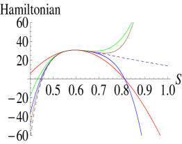
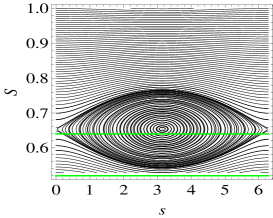
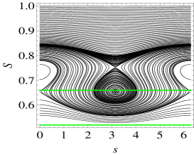
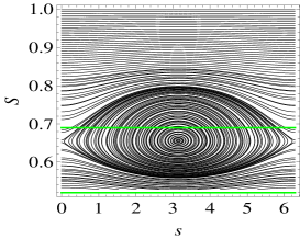
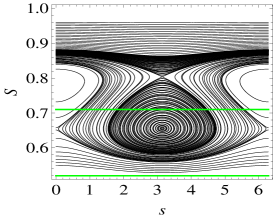
Figure 7. Resonance $-2\dot{\omega}+\dot{\Omega}=0$, case $i=69^{\circ}$. Upper left panel: graph of the true lunisolar Hamiltonian (dotted curve) and those of the truncated expansions ($2^{nd}$ red, $3^{rd}$ green, $4^{th}$ blue, $5^{th}$ brown) $s=\pi$, $L_{0}=1$, $T=0.5$. Upper middle panel: phase space portrait in the plane $(s,S)$ for the true Hamiltonian. Upper right panel: phase portrait for the $2^{nd}$ order expansion. Lower panels from left to right: phase portraits for the expansions to order 3, 4, 5.

6. Bifurcations of type $(i)$: critical inclination secular resonances

In this Section we investigate the secular resonances of type $(i)$, which are obtained by solving the equation $\dot{\omega}=0$. This resonance occurs at the so-called critical inclinations, whose values are $i=63.4^{\circ}$ and $i=116.4^{\circ}$ (see [29]). To be consistent with the previous notation, we make the trivial (identity) transformation of variables:

$$\sigma = \omega\ ,\qquad\ S=G\ ,$$

$$\eta = \Omega\ ,\qquad\ T=H\ .$$

We discuss just the case $i=63.4^{\circ}$, since the other one can be treated similarly.

It is important to stress that special care must be taken when dealing with such resonance. In fact, the equivalent of the Hamiltonian expansion in (4.9) up to second order provides only a rough result, when one compares the phase space portraits of the Hamiltonian expanded to second order and the full Hamiltonian.

To improve the results, we need to perform an expansion to higher order and therefore we proceed to expand up to order 5 in $S_{0}$. The equation for $\dot{S}=0$ provides the equilibrium values $s=0$ and $s=\pi/2$. On the other hand, the equation $\dot{s}=0$ for $s=0$ or $s=\pi/2$ provides a third–order equation in $S$. One finds that in both cases, namely $s=0$ and $s=\pi/2$, two solutions are complex conjugated, while the third solution is real. After an expansion in $T$ up to the order 6 of the real solutions, one can proceed as in Section 4.2 to compute the bifurcation values and the corresponding phase space portraits. In particular, for $i=63.4^{\circ}$, Figure 8 provides the bifurcation curves for $T_{A}$ and $T_{B}$ (see (4.13)) for the second (middle panel) and fourth (right panel) order expansions. The left panel of Figure 8 shows the contribution due just to the Sun.

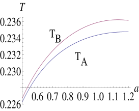
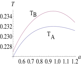
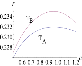
Figure 8. Critical inclination secular resonance. Plots of the bifurcation curves $T_{A}$, $T_{B}$ in (4.13) as a function of the semimajor axis for the case $i=63.4^{\circ}$. Left: the Hamiltonian includes just the effect of the Sun; middle: the Hamiltonian includes only the Moon with an expansion to order 2; right: the Hamiltonian includes only the Moon with an expansion to order 4.

The phase space portraits for the critical inclination case are presented in Figure 9. As in Section 5.1 we test the accuracy of the computations by comparing the truncations of the Hamiltonian with different degrees of expansion, from 2 to 5.

As already remarked in Figure 7, we notice that as the order of the expansion gets larger, the Hamiltonian graph is reproduced with a better accuracy. The interval where the true and expanded functions agree is reported within green lines in the phase portraits of Figure 9.

From an inspection of the true phase portrait given by the upper middle panel of Figure 9, we observe that the critical inclination case presents further equilibrium points (see the elliptic equilibria located at about $S=0.803$ for $s=0,\pi$). This phenomenon is close to what observed in the EFM2 model discussed in Remark 3.

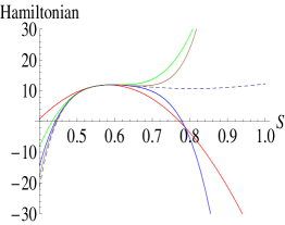
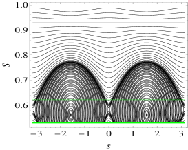
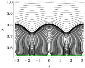
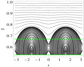
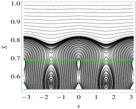
Figure 9. Critical inclination resonance, the case $i=63.4^{\circ}$. Phase space portraits in the plane $(s,S)$ with Sun and Moon included in the model. Upper left panel: graph of the true Hamiltonian (dotted curve) and those of the truncated expansions ($2^{nd}$ red, $3^{rd}$ green, $4^{th}$ blue, $5^{th}$ brown) $s=\pi$, $L_{0}=1$, $T=0.25$. Upper middle panel: phase space portrait in the plane $(s,S)$ for the true Hamiltonian. Upper right panel: phase portrait for the $2^{nd}$ order expansion. Lower panels from left to right: phase portraits for the expansions to order 3, 4, 5.

7. Bifurcations of type $(ii)$: polar secular resonances

In the case of polar resonances corresponding to $\dot{\Omega}=0$, the transformation of variables reduces to the identity:

$$\sigma = \Omega\ ,\qquad S=H\ ,$$

$$\eta = \omega\ ,\qquad\ T=G\ .$$

The treatment of polar resonances is made complicated by several factors. First of all, it is difficult to combine the effects of both the Moon and Sun, due to the fact that the corresponding expansions contain terms which are qualitatively different. On the other hand, even if we consider the effects of only one body, at the exact resonance one has $S=0$, so that the second order expansion of the Hamiltonian should be performed around $S_{0}=0$. Hence, one has (physical) bounds on $T$, but not on $S$ which is independent of $T$. Therefore the method can only be applied by deciding to impose a limitation to the range of variability of the $S$ coordinate, which in turn becomes a constraint on the variation of the inclination.

Let us proceed according to this strategy and assume to consider just the effect of the Moon. Then, the corresponding Hamiltonian takes the form

$${\mathcal{H}}_{Moon}^{polar}(S,T,s)=h_{0}(T)+S^{2}h_{1}(T)+S\ \sqrt{1-{S^{2}\over T^{2}}}\ f_{0}(T)\ \cos s+(g_{0}(T)+S^{2}g_{1}(T))\ \cos 2s$$

for some functions $h_{0}$, $h_{1}$, $f_{0}$, $g_{0}$, $g_{1}$ and for $s=\sigma-0.212$. After expanding to second order ${\mathcal{H}}_{Moon}^{polar}$ around $S_{0}=0$, one obtains

$${\mathcal{H}}_{Moon,exp}^{polar}(S,T,s)=h_{0}(T)+S^{2}h_{1}(T)+S\ f_{0}(T)\ \cos s+(g_{0}(T)+S^{2}g_{1}(T))\ \cos 2s\ .$$

Hence, the equations of motion are

$$\dot{S} = S\ f_{0}(T)\ \sin s+2\Big{(}g_{0}(T)+S^{2}g_{1}(T)\Big{)}\ \sin 2s$$

$$\dot{s} = f_{0}(T)\ \cos s+2S\Big{(}h_{1}(T)+g_{1}(T)\ \cos 2s\Big{)}\ .$$

Therefore, in addition to the two standard solutions $(S_{A},0)$ and $(S_{B},\pi)$ we have also a fixed (in the sense of being independent of $T$) pair of solutions, given by

$$S=0,\quad s=\pm\pi/2.$$

These elliptic equilibria do not play any role for generating new periodic orbits. However, they give a well definite shape to the structure of the phase space and in particular they determine the nature of the bifurcating families, since these are both stable. We then proceed to compute their locations in the plane $(S,s)$, using the technique implemented for the other resonances. To this end, we fix a value $S_{min}$ close to zero, say $S_{min}=0.01$. The computation of the bifurcation thresholds corresponding to $s=0$ and $s=\pi$ provides the values $T_{A}=0.313$ and $T_{B}=0.450$. Plotting the graphs between the lower threshold $S=0$ and an arbitrary upper limit, say $S=0.1$, we obtain the birth of equilibria for values like those shown in Figure 10.

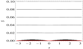
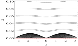
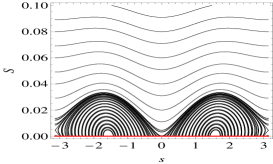
Figure 10. Polar secular resonance: phase space portraits corresponding to the GPS value $a=a_{GPS}$ in the plane $(s,S)$ for the Hamiltonian including the effect of the Moon: $T=0.2$ (left), $T=0.4$ (middle), $T=0.6$ (right).

8. Some remarks on the non–averaged problem

In Sections 4, 5, 6, 7, we have based our discussion on the analysis of the averaged system, described by a one–dimensional (averaged) Hamiltonian function, that we write in compact form as

$${\mathcal{H}}_{av}={\mathcal{H}}_{av}(S,T,\sigma)$$ (8.1)

(compare with (4.9) where $s$ is used in place of $\sigma$). The coordinates $(S,\sigma)$ admit, after the second bifurcation, a hyperbolic point, while $T$ is an integral of motion. For a given level $T=T_{0}$, the product of the hyperbolic point times the level set $T=T_{0}$ is a whiskered torus.

As $T$ varies we get a NHIM foliated by whiskered tori. Thus, we may wonder what happens when we add the perturbation to (8.1). We try to answer this question at least from a qualitative point of view, being aware that a quantitative analysis requires proper mathematical statements and several additional computations, which might be the object of study of a future work.

We start by noticing that the non–averaged system has the form

$${\mathcal{H}}_{nav}(S,T,\sigma,\eta)={\mathcal{H}}_{av}(S,T,\sigma)+\varepsilon{\mathcal{H}}_{p}(S,T,\sigma,\eta)\ ,$$ (8.2)

where ${\mathcal{H}}_{p}$ is the perturbing function, given by the part depending on the angles of $\overline{\mathcal{R}}_{Moon}^{(res)}$, $\overline{\mathcal{R}}_{Sun}^{(res)}$ in (4.3), (4.4), provided that $\Omega_{M}$, $\Omega_{S}$ are considered constants as in assumption H2. It turns out that the parameter $\varepsilon$ is of the order of the square of the eccentricity and therefore it can be considered small, at least for ranges of the coordinates that correspond to nearly circular orbits.

Given the expression of the Hamiltonian in (8.2), we may use a perturbation approach, which allows us to state that the NHIM persists for $\varepsilon$ small enough (see, e.g., [21, 22, 27, 39]). Under a suitable non–degeneracy condition and a Diophantine assumption on the frequency, the two–dimensional Hamiltonian ${\mathcal{H}}_{nav}={\mathcal{H}}_{nav}(S,T,\sigma,\eta)$ admits invariant tori ([33, 1, 37]), provided that $\varepsilon$ satisfies some smallness constraint. On a three–dimensional energy level, the two–dimensional KAM tori provide a stability property in the sense of confinement of the motion.

When the assumption on the constancy of the rates of variation of $\Omega_{M}$, $\Omega_{S}$ is removed, we end up with a non–autonomous Hamiltonian function of the form (4.2), that we can write as

$${\mathcal{H}}_{non-aut}(S,T,\sigma,\eta,t)={\mathcal{H}}_{av}(S,T,\sigma)+\varepsilon{\mathcal{H}}_{p}(S,T,\sigma,\eta)+\varepsilon{\mathcal{H}}_{t}(S,T,\sigma,\eta,\gamma t)\ ,$$ (8.3)

where ${\mathcal{H}}_{t}$ is the time–dependent part arising from the variation of the perturbers’ angular elements and $\gamma$ is a parameter depending on the rates of variation of the longitudes of the ascending nodes of the Moon and Sun. Precisely, $\gamma$ is nearly zero for the Sun and it is about equal to $-0.053^{\circ}/day$ for the Moon, thus showing that the time-dependent part due to the motion of the ascending node of the Moon is relevant on the time scale of about 18 years. The 2–dimensional, time–dependent Hamiltonian ${\mathcal{H}}_{non-aut}$ does not admit a confinement through KAM tori, since the phase space has dimension 5 and the KAM tori have dimension 3. A mechanism giving rise to Arnold’s diffusion ([2]) can be triggered by the existence of transition chains generated by the intersection of the unstable manifold of a torus and the stable manifold of another. The onset of Arnold’s diffusion is subject to the fulfillment of some non–degeneracy assumptions as well as some conditions on the so–called Melnikov’s integrals (see, e.g., [28]), ensuring the occurrence of transversal intersections. As an alternative to Melnikov’s method for the study of Arnold’s diffusion, one may compute the so–called scattering map ([18, 19]), which describes the behavior of the excursions between the tori.

9. Conclusions

The study of lunisolar resonances has raised a renewed interest, thanks to the increasing awareness of their effects on the space debris orbiting at different altitudes around our planet. Several works have underlined the importance of the influence of the Moon and Sun on objects located in MEO and GEO (see, e.g., [44]). Therefore, a careful investigation of lunisolar secular resonances is mandatory, also in view of practical applications.

A first step toward such investigation is represented by the analysis of those resonances which depend just on the inclination ([29]). These resonances occur in physically relevant regions, where several space debris are observed to orbit around the Earth.

Understanding the structure of the phase space, even for the simplest mathematical models as those considered in this work, can offer a simple explanation for the long-term evolution of space debris. For example, the long-term growth in eccentricity, observed for disposal orbits of various satellites, such as GPS, GLONASS, and GALILEO (see [13]), may be viewed as a natural effect of the lunisolar resonances. As shown by the phase–portraits in Figures 2, 7 and 9, and the FLI maps of Figures 4 and 5, inside the libration region, the action $S$ varies periodically. Since the eccentricity $e$ is related to $S$, it follows naturally that the eccentricity varies in time. Moreover, if the libration region take a large portion of the phase space, as in the top middle panel of Figure 9, then an orbit having a very small initial eccentricity (or $S\simeq 1$) could become a collision orbit.

Motivated by the intrinsic physical interest, we have analyzed the bifurcations associated with the lunisolar secular resonances; the model describing such resonances obviously includes also the effect of the geopotential. Our study supports that the role of the Moon is definitely relevant and cannot be neglected within a careful study of space debris dynamics (compare, e.g., with Figure 1). We have provided two methods to analyze the occurrence of bifurcations (see Sections 4.2 and 4.3). Both methods are fast and simple to implement; they provide the explicit values of the orbital elements at which two different bifurcations take place. Typically, the first bifurcation is associated to the birth of an elliptic equilibrium point for physically relevant values of the altitude (namely, above the Earth’s radius). The second bifurcation shows the occurrence of the elliptic equilibrium point together with a pair of hyperbolic equilibria.

Care must be taken in analyzing the different classes of lunisolar resonances. In fact, it should be stressed that when the inclination is such that one resonant variable becomes degenerate, then the method fails. Moreover, in some cases a higher accuracy is necessary to get reliable results. This means that the expansions of the Hamiltonian describing the model must be computed to higher orders as in the case, e.g., of the critical inclination secular resonance. In all these cases we have pitchfork bifurcations of two different families, the first being stable and the second unstable. A peculiar case is represented by polar orbits, where both bifurcating families are stable.

As a conclusive remark, we underline that a mathematical study of the existence of equilibria is also of practical interest. In fact, the elliptic points and their neighboring orbits represent phase space regions where one could stably place an object, while hyperbolic equilibria provide unstable regions, where the objects can be placed to experience large excursions in phase space through the stable and unstable manifolds associated with the hyperbolic dynamics.

Acknowledgements. We are grateful to Christoph Lhotka, Alessandro Rossi, Tere Seara, and Alfonso Sorrentino for very useful discussions and suggestions.

References

- [1] V.I. Arnold, Proof of a theorem of A. N. Kolmogorov on the invariance of quasi-periodic motions under small perturbations, Russian Math. Surveys 18, 9–36 (1963)
- [2] V.I. Arnold, Instability of dynamical systems with several degrees of freedom, Sov. Math. Doklady 5, 581–585 (1964)
- [3] S. Belyanin, P. Gurfil, Semianalytical study of geosynchronous orbits about a precessing oblate Earth under lunisolar gravitation and tesseral resonance, J. Astronautical Sc. 57, n.3, 517–543 (2009)
- [4] S. Breiter, Lunisolar apsidal resonances at low satellite orbits, Celest. Mech. Dyn. Astr. 74, 253–274 (1999)
- [5] S. Breiter, On the coupling of lunisolar resonances for Earth satellite orbits, Celest. Mech. Dyn. Astr. 80, 1–20 (2001)
- [6] S. Breiter, Lunisolar resonances revisited, Celest. Mech. Dyn. Astr. 81, 81–91 (2001)
- [7] A. Celletti, Stability and Chaos in Celestial Mechanics, Springer-Verlag, Berlin; published in association with Praxis Publishing Ltd., Chichester, ISBN: 978-3-540-85145-5 (2010)
- [8] A. Celletti, C. Galeş, On the dynamics of space debris: 1:1 and 2:1 resonances, J. Nonlinear Science 24, n. 6, 1231–1262 (2014)
- [9] A. Celletti, C. Galeş, Dynamical investigation of minor resonances for space debris, Celest. Mech. Dyn. Astr. 123, n. 2, 203-222 (2015)
- [10] A. Celletti, C. Galeş, G. Pucacco, A. Rosengren, Analytical development of the lunisolar disturbing function and the critical inclination secular resonance, arXiv:1511.03567, (2015)
- [11] A. Celletti, G. Pucacco, D. Stella, Lissajous and Halo orbits in the restricted three-body problem, J. Nonlinear Science 25, Issue 2, 343–370 (2015)
- [12] C.C. Chao, Applied Orbit Perturbation and Maintenance, Aerospace Press Series, AIAA, Reston, Virgina (2005)
- [13] C.C. Chao, R.A. Gick, Long-term evolution of navigation satellite orbits: GPS/GLONASS/GALILEO, Advan. Space Res., 34, 1221–1226 (2004)
- [14] S. L. Coffey, A. Deprit, B. R. Miller, The critical inclination in artificial satellite theory, Celest. Mech. 39, 365–406 (1986)
- [15] S. L. Coffey, A. Deprit, E. Deprit, L. Healey, Painting the phase space portrait of an integrable dynamical system, Science 247, 833–836 (1989)
- [16] J. Daquin, A.J. Rosengren, E.M. Alessi, F. Deleflie, G.B. Valsecchi, A. Rossi, The dynamical structure of the MEO region: long-term stability, chaos, and transport, Celest. Mech. Dyn. Astr. 124, 335–366 (2016)
- [17] F. Deleflie, A. Rossi, C. Portmann, G. Me tris, F. Barlier, Semi-analytical investigations of the long term evolution of the eccentricity of Galileo and GPS-like orbits, Advances in Space Research, 47, 811–821 (2011)
- [18] A. Delshams, R. de la Llave, T.M. Seara, A geometric approach to the existence of orbits with unbounded energy in generic periodic perturbations by a potential of generic geodesic flows of , Comm. Math. Phys. 209, n. 2, 353 -392 (2000)
- [19] A. Delshams, R. de la Llave, T.M. Seara, Geometric properties of the scattering map of a normally hyperbolic invariant manifold, Advances in Mathematics 217, 1096 -1153 (2008)
- [20] T.A. Ely, K.C. Howell, Dynamics of artificial satellite orbits with tesseral resonances including the effects of luni–solar perturbations, Dynamics and Stability of Systems 12, n. 4, 243–269 (1997)
- [21] N. Fenichel, Persistence and smoothness of invariant manifolds for flows, Indiana Univ. Math. J. 21, 193–226 (1971-1972)
- [22] N. Fenichel, Asymptotic stability with rate conditions, Indiana Univ. Math. J. 23, 1109–1137 (1973-1974)
- [23] C. Froeschlé, E. Lega, R. Gonczi, Fast Lyapunov indicators. Application to asteroidal motion, Celest. Mech. Dyn. Astr., 67, 41–62 (1997)
- [24] G.E.O. Giacaglia, Lunar perturbations of artificial satellites of the Earth, Celest. Mech. 9, 239–267 (1974)
- [25] G.E.O. Giacaglia, A note on Hansen’s coefficients in satellite theory, Celest. Mech. 14, 515–523 (1976)
- [26] J. Henrard, A. Lemaître, A second fundamental model for resonance, Celest. Mech. 30, 197–218 (1983)
- [27] M.W. Hirsch, C.C. Pugh, M. Shub, Invariant manifolds, Lecture Notes in Mathematics 583, Springer-Verlag, Berlin (1977)
- [28] P.H. Holmes, J.E. Marsden, Melnikov’s method and Arnold diffusion for perturbations of integrable Hamiltonian systems, J. Math. Phys. 23, 669–675 (1982)
- [29] S. Hughes, Earth Satellite Orbits with Resonant Lunisolar Perturbations. I. Resonances Dependent Only on Inclination, Proc. R. Soc. Lond. A 372, 243–264 (1980)
- [30] S. Hughes, Earth Satellite Orbits with Resonant Lunisolar Pertubations II. Some Resonances Dependent on the Semi-Major Axis, Eccentricity and Inclination, Proc. R. Soc. Lond. A 375, 379–396 (1981)
- [31] W.M. Kaula, Developement of the lunar and solar disturbing functions for a close satellite, The Astronomical Journal 67, 300–303 (1962)
- [32] W.M. Kaula, Theory of Satellite Geodesy, Blaisdell Publ. Co. (1966)
- [33] A. N. Kolmogorov, On conservation of conditionally periodic motions for a small change in Hamilton’s function, Dokl. Akad. Nauk SSSR (N.S.) 98, 527–530 (1954)
- [34] M.T. Lane, On analytic modeling of lunar perturbations of artifical satellites of the Earth, Celest. Mech. Dyn. Astr. 46, 287–305 (1989)
- [35] A. Lemaître, High-order resonances in the restricted three-body problem, Celest. Mech. 32, 109–126 (1984)
- [36] A. Lemaître, N. Delsate, S. Valk, A web of secondary resonances for large geostationary debris, Celest. Mech. Dyn. Astr. 104, 383–402 (2009)
- [37] J. Moser, On invariant curves of area-preserving mappings of an annulus, Nachr. Akad. Wiss. Göttingen Math.-Phys. Kl. II, 1–20 (1962)
- [38] C.D. Murray, S.F Dermott, Solar system dynamics, Cambridge University Press (1999)
- [39] Ya. B. Pesin, Lectures on partial hyperbolicity and stable ergodicity, Zürich Lectures in Advanced Mathematics, European Mathematical Society (EMS), Zürich (2004)
- [40] A. Marchesiello, G. Pucacco, Relevance of the 1:1 resonance in galactic dynamics, Eur. Phys. J. Plus 126, 104–118 (2011)
- [41] A. Marchesiello, G. Pucacco, Equivariant singularity analysis of the 2:2 resonance, Nonlinearity, 27, 43–66 (2014)
- [42] G. Pucacco, A. Marchesiello, An energy-momentum map for the time-reversal symmetric 1:1 resonance with symmetry, Physica D 271, 10–18 (2014)
- [43] A.J. Rosengren, E.M. Alessi, A. Rossi, G.B. Valsecchi, Chaos in navigation satellite orbits caused by the perturbed motion of the Moon, Monthly Notices of the Royal Astronomical Society, 449, 3522–3526 (2015)
- [44] A. Rossi, Resonant dynamics of Medium Earth Orbits: space debris issues, Celest. Mech. Dyn. Astr. 100, 267–286 (2008)
- [45] J.L. Simon, P. Bretagnon, J. Chapront, M, Chapront–Touzé, G. Francou, J. Laskar, Numerical expressions for precession formulae and mean elements for the Moon and the planets, Astron. Astrophys. 282, 663–683 (1994)
- [46] S. Valk, A. Lemaître, Analytical and semi-analytical investigations of geosynchronous space debris with high area-to-mass ratios, Advances in Space Research 41, 1077–1090 (2008)
- [47] S. Valk, A. Lemaître, F. Deleflie, Semi-analytical theory of mean orbital motion for geosynchronous space debris under gravitational influence, Advances in Space Research, 43, 1070–1082 (2009)