Minimax Estimation of a Functional on a Structured High-dimensional Model (corrected version)

Abstract

We introduce a new method of estimation of parameters in semiparametric and nonparametric models. The method is based $U$-statistics that are based on higher order influence functions that extend ordinary linear influence functions of the parameter of interest, and represent higher derivatives of this parameter. For parameters for which the representation cannot be perfect the method often leads to a bias-variance trade-off, and results in estimators that converge at a slower than $\sqrt{n}$-rate. In a number of examples the resulting rate can be shown to be optimal. We are particularly interested in estimating parameters in models with a nuisance parameter of high dimension or low regularity, where the parameter of interest cannot be estimated at $\sqrt{n}$-rate, but we also consider efficient $\sqrt{n}$-estimation using novel nonlinear estimators. The general approach is applied in detail to the example of estimating a mean response when the response is not always observed.

Abstract

This supplement contains the proof of Theorem 9.1 in the case that $m>3$, and it contains three appendices.

July 2022

1 Introduction

Let $X_{1},X_{2},\ldots,X_{n}$ be a random sample from a density $p$ relative to a measure ${\mu}$ on a sample space $({\cal X},{\cal A})$. It is known that $p$ belongs to a collection ${\cal P}$ of densities, and the problem is to estimate the value $\chi(p)$ of a functional $\chi:{\cal P}\to\mathbb{R}$. Our main interest is in the situation of a semiparametric or nonparametric model, where ${\cal P}$ is infinite dimensional, and especially in the case when the model is described through parameters of low regularity. In this case the parameter $\chi(p)$ may not be estimable at the “usual” $\sqrt{n}$-rate.

In low-dimensional semiparametric models estimating equations have been found a good strategy for constructing estimators [2, 34, 40]. In our present setting it will be more convenient to consider one-step versions of such estimators, which take the form

$$\hat{\chi}_{n}=\chi(\hat{p}_{n})+\mathbb{P}_{n}\chi_{\hat{p}_{n}},$$ (1.1)

for $\hat{p}_{n}$ an initial estimator for $p$ and $x\mapsto\chi_{p}(x)$ a given measurable function, for each $p\in{\cal P}$, and $\mathbb{P}_{n}f$ short hand notation for $n^{-1}{\sum_{i=1}^{n}}f(X_{i})$.

One possible choice in (1.1) is $\chi_{p}=0$, leading to the plug-in estimator $\chi(\hat{p}_{n})$. However, unless the initial estimator $\hat{p}_{n}$ possesses special properties, this choice is typically suboptimal. Better functions $\chi_{p}$ can be constructed by consideration of the tangent space of the model. To see this, we write (with $P\chi_{\hat{p}}$ shorthand for $\int\chi_{\hat{p}}(x)\,dP(x)$)

$$\hat{\chi}_{n}-\chi(p)=\bigl{[}\chi(\hat{p}_{n})-\chi(p)+P\chi_{\hat{p}_{n}}\bigr{]}+(\mathbb{P}_{n}-P)\chi_{\hat{p}_{n}}.$$ (1.2)

Because it is properly centered, we may expect the sequence $\sqrt{n}(\mathbb{P}_{n}-P)\chi_{\hat{p}_{n}}$ to tend in distribution to a mean-zero normal distribution. The term between square brackets on the right of (1.2), which we shall refer to as the bias term, depends on the initial estimator $\hat{p}_{n}$, and it would be natural to construct the function $\chi_{p}$ such that this term does not contribute to the limit distribution, or at least is not dominating the expression. Thus we would like to choose this function such that the “bias term” is no bigger than of the order $O_{P}(n^{-1/2})$. A good choice is to ensure that the term $P\chi_{\hat{p}_{n}}$ acts as minus the first derivative of the functional $\chi$ in the “direction” $\hat{p}_{n}-p$. Functions $x\mapsto\chi_{p}(x)$ with this property are known as influence functions in semiparametric theory [16, 22, 35, 5, 2], go back to the von Mises calculus due to [33], and play an important role in robust statistics [14, 11], or [40], Chapter 20.

For an influence function we may expect that the “bias term” is quadratic in the error $d(\hat{p}_{n},p)$, for an appropriate distance $d$. In that case it is certainly negligible as soon as this error is of order $o_{P}(n^{-1/4})$. Such a “no-bias” condition is well known in semiparametric theory (e.g. condition (25.52) in [40] or (11) in [20]). However, typically it requires that the model ${\cal P}$ be “not too big”. For instance, a regression or density function on $d$-dimensional space can be estimated at rate $n^{-1/4}$ if it is a-priori known to have at least $d/2$ derivatives (indeed ${\alpha}/(2{\alpha}+d)\geq 1/4$ if ${\alpha}\geq d/2$). The purpose of this paper is to develop estimation procedures for the case that no estimators exist that attain a $O_{P}(n^{-1/4})$ rate of convergence. The estimator (1.1) is then suboptimal, because it fails to make a proper trade-off between “bias” and “variance”: the two terms in (1.2) have different magnitudes. Our strategy is to replace the linear term $\mathbb{P}_{n}\chi_{p}$ by a general $U$-statistic $\mathbb{U}_{n}\chi_{p}$, for an appropriate $m$-dimensional influence function $(x_{1},\ldots,x_{m})\mapsto\chi_{p}(x_{1},\ldots,x_{m})$, chosen using a type of von Mises expansion of $p\mapsto\chi(p)$. Here the order $m$ is adapted to the size of the model ${\cal P}$ and the type of functional to be estimated.

Unfortunately, “exact” higher-order influence functions turn out to exist only for special functionals $\chi$. To treat general functionals $\chi$ we approximate these by simpler functionals, or use approximate influence functions. The rate of the resulting estimator is then determined by a trade-off between bias and variance terms. It may still be of order $1/\sqrt{n}$, but it is typically slower. In the former case, surprisingly, one may obtain semiparametric efficiency by estimators whose variance is determined by the linear term, but whose bias is corrected using higher order influence functions. The latter case will be of more interest.

The conclusion that the “bias term” in (1.2) is quadratic in the estimation error $d(\hat{p}_{n},p)$ is based on a worst case analysis. First, there exist a large number of models and functionals of interest that permit a first order influence function that is unbiased in the nuisance parameter. (E.g. adaptive models as considered in [1], models allowing a sufficient statistic for the nuisance parameter as in [38, 39], mixture models as considered in [19, 24, 36], and convex-linear models in survival analysis.) In such models there is no need for higher-order influence functions. Second, the analysis does not take special, structural properties of the initial estimators $\hat{p}_{n}$ into account. An alternative approach would be to study the bias of a particular estimator in detail, and adapt the influence function to this special estimator. The strategy in this paper is not to use such special properties and focus on influence functions that work with general initial estimators $\hat{p}_{n}$.

The motivation for our new estimators stems from studies in epidemiology and econometrics that include covariates whose influence on an outcome of interest cannot be reliably modelled by a simple model. These covariates may themselves not be of interest, but are included in the analysis to adjust the analysis for possible bias. For instance, the mechanism that describes why certain data is missing is in terms of conditional probabilities given several covariates, but the functional form of this dependence is unknown. Or, to permit a causal interpretation in an observational study one conditions on a set of covariates to control for confounding, but the form of the dependence on the confounding variables is unknown. One may hypothesize in such situations that the functional dependence on a set of (continuous) covariates is smooth (e.g. $d/2$ times differentiable in the case of $d$ covariates), or even linear. Then the usual estimators will be accurate (at order $O_{P}(n^{-1/2})$) if the hypothesis is true, but they will be badly biased in the other case. In particular, the usual normal-theory based confidence intervals may be totally misleading: they will be both too narrow and wrongly located. The methods in this paper yield estimators with (typically) wider corresponding confidence intervals, but they are correct under weaker assumptions.

The mathematical contributions of the paper are to provide a heuristic for constructing minimax estimators in semiparametric models, and to apply this to a concrete model, which is a template for a number of other models (see [27, 37]). The methods connect to earlier work [13, 21] on the estimation of functionals on nonparametric models, but differ by our focus on functionals that are defined in terms of the structure of a semiparametric model. This requires an analysis of the inverse map from the density of the observations to the parameters, in terms of the semiparametric tangent spaces of the models. Our second order estimators are related to work on quadratic functionals, or functionals that are well approximated by quadratic functionals, as in [10, 15, 3, 4, 17, 18, 6, 7]. While we place the construction of minimax estimators for these special functionals in a wider framework, our focus differs by going beyond quadratic estimators and to consider semiparametric models.

Our mathematical results are in part conditional on a scale of regularity parameters (through the dimension given in (9.9) and a partition of this dimension that depends on two of these parameters). We hope to discuss adaptation to these parameters in future work.

General heuristics of our construction are given in Section 4. Sections 5–9 are devoted to constructing new estimators for the mean response effect in missing data problems. The latter are introduced in Section 3, so that they can serve as illustration to the general heuristics in Section 4. In Section 11 (in the supplement [26]) we briefly discuss other problems, including estimating a density at a point, where already first order influence functions do not exist and our heuristics naturally lead to projection estimators, and estimating a quadratic functional, where our approach produces standard estimators from the literature in a natural way. Section 10 (partly in the supplement [26]) collects technical proofs. Sections 12, 13 and 14 (in the supplement [26]) discuss three key concepts of the paper: influence functions, projections and $U$-statistics.

2 Notation

Let $\mathbb{U}_{n}$ denote the empirical $U$-statistic measure, viewed as an operator on functions. For given $m\leq n$ and a function $f:{\cal X}^{m}\to\mathbb{R}$ on the sample space this is defined by

$$\mathbb{U}_{n}f=\frac{1}{n(n-1)\cdots(n-m+1)}\mathop{\mathchar 4944\relax\mathchar 4944\relax\cdots\mathchar 4944\relax}\limits_{1\leq i_{1}\not=i_{2}\not=\cdots\not=i_{m}\leq n}f(X_{i_{1}},X_{i_{2}},\cdots,X_{i_{m}}).$$

We do not let the order $m$ show up in the notation $\mathbb{U}_{n}f$. This is unnecessary, as the notation is consistent in the following sense: if a function $f:{\cal X}^{l}\to\mathbb{R}$ of $l<m$ arguments is considered a function of $m$ arguments that is constant in its last $m-l$ arguments, then the right side of the preceding display is well defined and is exactly the corresponding $U$-statistic of order $l$. In particular, $\mathbb{U}_{n}f$ is the empirical distribution $\mathbb{P}_{n}$ applied to $f$ if $f:{\cal X}\to\mathbb{R}$ depends on only one argument.

We write $P^{n}\mathbb{U}_{n}f=P^{m}f$ for the expectation of $\mathbb{U}_{n}f$ if $X_{1},\ldots,X_{n}$ are distributed according to the probability measure $P$, and for the expectation of $f$ under the product measure $P^{m}$ of $m$ copies of $P$. We also use this operator notation for the expectations of statistics in general. If the distribution of the observations is given by a density $p$, then we use $P$ as the measure corresponding to $p$, and use the preceding notations likewise. Finally $\mathbb{U}_{n}-P^{m}$ denotes the centered $U$-statistic empirical measure, defined by $(\mathbb{U}_{n}-P^{m})f=\mathbb{U}_{n}f-P^{m}f$, for any integrable function $f$.

We call $f$ degenerate relative to $P$ if $\int f(x_{1},\ldots,x_{m})\,dP(x_{i})=0$ for every $i$ and every $(x_{j}:j\not=i)$, and we call $f$ symmetric if $f(x_{1},\ldots,x_{m})$ is invariant under permutation of the arguments $x_{1},\ldots,x_{m}$. Given an arbitrary measurable function $f:{\cal X}^{m}\rightarrow\mathbb{R}$ we can form a function that is degenerate relative to $P$ by subtracting the orthogonal projection in $L_{2}(P^{m})$ onto the functions of at most $m-1$ variables. This degenerate function can be written in the form (e.g. [40], Lemma 11.11)

$$(D_{P}f)(X_{1},\ldots,X_{m}) \!=\!\!\!\!\!\!\sum_{A\subset\{1,\ldots,m\}}\!\!\!\!\!(-1)^{m-|A|}\mathord{\rm E}_{P}\Bigl{[}f(X_{1},\ldots,X_{m})\mathchar 25194\relax X_{i}:i\in A\Bigr{]},\!\!$$ (2.1)

where the sum is over all subsets $A$ of $\{1,\ldots,m\}$, including the empty set. Here the conditional expectation $\mathord{\rm E}\bigl{[}f(X_{1},\ldots,X_{m})\mathchar 25194\relax X_{i}:i\in\emptyset\bigr{]}$ is understood to be the unconditional expectation $\mathord{\rm E}f(X_{1},\ldots,X_{m})=P^{m}f$. If the function $f$ is symmetric, then so is the function $D_{P}f$.

Given two functions $g,h:{\cal X}\to\mathbb{R}$ we write $g\times h$ for the function $(x,y)\mapsto g(x)h(y)$. More generally, given $m$ functions $g_{1},\ldots,g_{m}$ we write $g_{1}\times\cdots\times g_{m}$ for the tensor product of these functions. Such product functions are degenerate iff all functions in the product have mean zero.

A kernel operator $K:L_{r}({\cal X},{\cal A},{\mu})\to L_{r}({\cal X},{\cal A},{\mu})$ takes the form $(Kf)(x)=\int\bar{K}(x,y)f(y)\,d{\mu}(y)$ for some measurable function $\bar{K}:{\cal X}^{2}\to\mathbb{R}$. We shall abuse notation in denoting the operator $K$ and the kernel $\bar{K}$ with the same symbol: $K=\bar{K}$. A (weighted) projection onto a finite-dimensional space is a kernel operator. We discuss such projections in Section 13.

The set of measurable functions whose $r$th absolute power is ${\mu}$-integrable is denoted $L_{r}({\mu})$, with norm $\|\cdot\|_{r,{\mu}}$, or $\|\cdot\|_{r}$ if the measure is clear; or also as $L_{r}(w)$ with norm $\|\cdot\|_{r,w}$ if $w$ is a density relative to a given dominating measure. For $r=\infty$ the notation $\|\cdot\|_{\infty}$ refers to the uniform norm.

3 Estimating the mean response in missing data models

In this section we introduce our main example, which will be used as a running example in the next section. We also summarize the results obtained for this example in the remainder of the paper.

Suppose that a typical observation is distributed as $X=(YA,A,Z)$, for $Y$ and $A$ taking values in the two-point set $\{0,1\}$ and conditionally independent given $Z$.

This model is standard in biostatistical applications, with $Y$ an “outcome” or “response variable”, which is observed only if the indicator $A$ takes the value $1$. The covariate $Z$ is chosen such that it contains all information on the dependence between the response and the missingness indicator $A$, thus making the response missing at random. Alternatively, we think of $Y$ as a “counterfactual” outcome if a treatment were given ($A=1$) and estimate (half) the treatment effect under the assumption of no unmeasured confounders. (The results also apply without the “missing-at-random” assumption, but with a different interpretation; see Remark 3.1.)

The model can be parameterized by the marginal density $f$ of $Z$ (relative to some dominating measure ${\nu}$) and the probabilities $b(z)=\mathord{\rm P}(Y=1\mathchar 25194\relax Z=z)$ and $a(z)^{-1}=\mathord{\rm P}(A=1\mathchar 25194\relax Z=z)$. (Using $a$ for the inverse probability simplifies later formulas.) Alternatively, the model can be parameterized by the pair $(a,b)$ and the function $g=f/a$, which is the conditional density of $Z$ given $A=1$, up to the norming factor $\mathord{\rm P}(A=1)$. Thus the density $p$ of an observation $X$ is described by the triplet $(a,b,f)$, or equivalently the triplet $(a,b,g)$. For simplicity of notation we write $p$ instead of $p_{a,b,f}$ or $p_{a,b,g}$, with the implicit understanding that a generic $p$ corresponds one-to-one to a generic $(a,b,f)$ or $(a,b,g)$.

We wish to estimate the mean response $\mathord{\rm E}Y=\mathord{\rm E}b(Z)$, i.e. the functional

$$\chi(p)=\int bf\,d{\nu}=\int abg\,d{\nu}.$$

Estimators that are $\sqrt{n}$-consistent and asymptotically efficient in the semiparametric sense have been constructed using a variety of methods (e.g. [30, 31], or see Section 5), but only if $a$ or $b$, or both, parameters are restricted to sufficiently small regularity classes. For instance, if the covariate $Z$ ranges over a compact, convex subset ${\cal Z}$ of $\mathbb{R}^{d}$, then the mentioned papers provide $\sqrt{n}$-consistent estimators under the assumption that $a$ and $b$ belong to Hölder classes $C^{\alpha}({\cal Z})$ and $C^{\beta}({\cal Z})$ with ${\alpha}$ and ${\beta}$ large enough that

$$\frac{{\alpha}}{2{\alpha}+d}+\frac{{\beta}}{2{\beta}+d}\geq\frac{1}{2}.$$ (3.1)

(See e.g. Section 2.7.1 in [41] for the definition of Hölder classes.) For moderate to large dimensions $d$ this is a restrictive requirement. In the sequel we consider estimation for arbitrarily small ${\alpha}$ and ${\beta}$.

3.1 Summary of results

Throughout we assume that the parameters $a$, $b$ and $g$ are contained in Hölder spaces $C^{\alpha}({\cal Z})$, $C^{\beta}({\cal Z})$ and $C^{\gamma}({\cal Z})$ of functions on a compact, convex domain in $\mathbb{R}^{d}$. We derive two types of results:

1. In Section 8 we show that a $\sqrt{n}$-rate is attainable by using a higher order influence function (of order determined by ${\gamma}$) as long as

   $$\frac{{\alpha}+{\beta}}{2}\geq\frac{d}{4}.$$ (3.2)

   This condition is strictly weaker than the condition (3.1) under which the linear estimator attains a $\sqrt{n}$-rate. Thus even in the $\sqrt{n}$-situation higher order estimating equations may yield estimators that are applicable in a wider range of models. For instance, in the case that ${\alpha}={\beta}$ the cut-off (3.1) arises for ${\alpha}={\beta}\geq d/2$, whereas (3.2) reduces to ${\alpha}={\beta}\geq d/4$.

2. We consider minimax estimation in the case $({\alpha}+{\beta})/2<d/4$, when the rate becomes slower than $1/\sqrt{n}$. It is shown in [29] that even if $g=f/a$ were known, then the minimax rate for $a$ and $b$ ranging over balls in the Hölder classes $C^{\alpha}({\cal Z})$ and $C^{\beta}({\cal Z})$ cannot be faster than $n^{-(2{\alpha}+2{\beta})/(2{\alpha}+2{\beta}+d)}$. In Section 9 we show that this rate is attainable if $g$ is known, and also if $g$ is unknown, but is a-priori known to belong to a Hölder class $C^{\gamma}({\cal Z})$ for sufficiently large ${\gamma}$, as given by (9.11). (Heuristic arguments, not discussed in this paper, appear to indicate that for smaller ${\gamma}$ the minimax rate is slower than $n^{-(2{\alpha}+2{\beta})/(2{\alpha}+2{\beta}+d)}$.)

We start by discussing the first and second order estimators in Sections 5 and 6, where the first is merely a summary of well known facts, but the second already contains some key elements of the new approach of the present paper. The preceding results (a) and (b) are next obtained in Sections 8 ($\sqrt{n}$-rate if $({\alpha}+{\beta})/2\geq d/4$) and 9 (slower rate if $({\alpha}+{\beta})/2<d/4$), using the higher-order influence functions of an approximate functional, which is defined in the intermediate Section 7. In the next section we discuss the general heuristics of our approach.

Assumption 3.1.

We assume throughout that the functions $1/a,b,g$ and their preliminary estimators $1/\hat{a},\hat{b},\hat{g}$ are bounded away from their extremes: 0 and 1 for the first two, and 0 and $\infty$ for the third.

Remark 3.1.

The assumption that the responses are “missing at random (MAR)” is used to identify the mean response functional. Without this assumption the results of the paper are still valid, but concern the functional $\int b_{1}(z)f(z)\,dz$, in which $b_{1}(z)=\mathord{\rm E}(Y\mathchar 25194\relax A=1,Z=z)$ has taken the place of $b(z)=\mathord{\rm E}(Y\mathchar 25194\relax Z=z)$, two functions that are identical under MAR. This follows from the fact that the likelihoods of $X=(YA,A,Z)$ without or with assuming MAR take exactly the same form, as given in (4.5), but with $b$ replaced by $b_{1}$. After this replacement all results go through. However, the functional $\int b_{1}(z)f(z)\,dz$ has the interpretation of the mean response only when MAR holds.

4 General heuristics

Our basic estimator has the form (1.1) except that we replace the linear term by a general $U$-statistic. Given measurable functions $\chi_{p}:{\cal X}^{m}\to\mathbb{R}$, for a fixed order $m$, we consider estimators $\hat{\chi}_{n}$ of $\chi(p)$ of the type

$$\hat{\chi}_{n}=\chi(\hat{p}_{n})+\mathbb{U}_{n}\chi_{\hat{p}_{n}}.$$ (4.1)

The initial estimators $\hat{p}_{n}$ are thought to have a certain (optimal) convergence rate $d(\hat{p}_{n},p)\rightarrow 0$, but need not possess (further) special properties. Throughout we shall treat these estimators as being based on an independent sample of observations, so that $\hat{p}_{n}$ and $\mathbb{U}_{n}$ in (4.1) are independent. This takes away technical complications, and allows us to focus on rates of estimation in full generality. (A simple way to avoid the resulting asymmetry would be to swap the two samples, calculate the estimator a second time and take the average.)

4.1 Influence functions

The key is to find suitable “influence functions” $\chi_{p}$. A decomposition of type (1.2) for the estimator (4.1) yields

$$\hat{\chi}_{n}-\chi(p)=\bigl{[}\chi(\hat{p}_{n})-\chi(p)+P^{m}\chi_{\hat{p}_{n}}\bigr{]}+(\mathbb{U}_{n}-P^{m})\chi_{\hat{p}_{n}}.$$ (4.2)

This suggests to construct the influence functions such that $-P^{m}\chi_{\hat{p}_{n}}$ represents the first $m$ terms of the Taylor expansion of $\chi(\hat{p}_{n})-\chi(p)$. We shall translate this requirement into a manageable form, and next work it out in detail for the missing data problem.

First the requirement implies that the influence function used in (4.1) must be unbiased:

$$P^{m}\chi_{p}=0.$$ (4.3)

Next, to operationalize a “Taylor expansion” on the (infinite-dimensional) “manifold” ${\cal P}$ we employ “smooth” submodels $t\mapsto p_{t}$. These are defined as maps from a neighbourhood of $0\in\mathbb{R}$ to ${\cal P}$ that pass through $p$ at $t=0$ (i.e. $p_{0}=p$) such that the derivatives in the following exist. For a large model there will be many such submodels, approaching $p$ from various “directions”. Given a collection of submodels we determine $\chi_{p}$ such that, for each submodel $t\mapsto p_{t}$,

$$\frac{d^{j}}{dt^{j}}_{|t=0}\chi(p_{t})=-\frac{d^{j}}{dt^{j}}_{|t=0}P^{m}\chi_{p_{t}},\qquad j=1,\ldots,m.$$

The subscript $|t=0$ on the differential quotients means “derivative evaluated at $t=0$”, i.e. at $p=p_{0}$. A slight strengthening is to impose this condition “everywhere” on the path, i.e. the $j$th derivative of $t\mapsto\chi(p_{t})$ at $t$ is the $j$th derivative of $h\mapsto-P_{t}^{m}\chi_{p_{t+h}}$ at $h=0$, for every $t$. (Here $P_{t}$ is the measure corresponding to the density $p_{t}$ and $P_{t}^{m}f$ the expectation of a function $f$ under the $m$-fold product of these measures.) If the map $(s,t)\mapsto P_{s}^{m}\chi_{p_{t}}$ is smooth, then the latter implies (cf. Lemma 12.1 applied with $\chi=f$ and $g(s,t)=-P_{t}^{m}\chi_{p_{s}}$)

$$\frac{d^{j}}{dt^{j}}_{|t=0}\chi(p_{t})=\frac{d^{j}}{dt^{j}}_{|t=0}P_{t}^{m}\chi_{p},\qquad j=1,\ldots,m.$$ (4.4)

Relative to the previous formula the subscript $t$ on the right hand side has changed places, and the negative sign has disappeared. This is similar to the “Bartlett equalities” familiar from manipulating expectations of scores and their higher derivatives. We take this equation together with unbiasedness as the defining property. Thus a measurable function $\chi_{p}:{\cal X}^{m}\to\mathbb{R}$ is said to be an $m$th order influence function at $p$ of the functional $p\mapsto\chi(p)$ relative to a given collection of one-dimensional submodels $t\mapsto p_{t}$ (with $p_{0}=p$) if it satisfies (4.3) and (4.4), for every submodel under consideration.

Equation (4.4) implies a Taylor expansion of $t\mapsto\chi(p_{t})$ at $t=0$ of order $m$, but in addition requires that the derivatives of this map can be represented as expectations involving a function $\chi_{p}$. The latter is made operational by requiring the derivatives to be identical to those of the map $t\mapsto P_{t}^{m}\chi_{p}$, which automatically have the desired representation. The representation as an expectation is essential for the construction of estimators. For exploiting derivatives up to the $m$th order, groups of $m$ observations can be used to match the expectation $P^{m}$; this leads to $U$-statistics of order $m$.

It is also essential that the expectation is relative to the law of the observations $X_{1},\ldots,X_{n}$. In a structured model, such as the missing data problem, the law $P_{\eta}$ of the observations depends on a parameter $\eta$ and the functional of interest is a quantity $\psi(\eta)$ defined in term of $\eta$. Then the representation requires to represent the derivative of the map $\eta\mapsto\psi(\eta)$ as an expectation relative to $P_{\eta}$. An expansion of just $\eta\mapsto\psi(\eta)$ without reference to the data distribution is not sufficient. Expressing the derivates in $P_{\eta}$ implicitly utilises the inverse map $P_{\eta}\mapsto\eta$, but by directly defining the influence function by (4.4) we sidestep an expansion of $\eta\mapsto\psi(\eta)$ and explicit inversion of the latter map.

We allow that there may be more than one influence function. In particular, we do not require $\chi_{p}$ in (4.4) to be symmetric in its arguments, although a given influence function can always be symmetrized without loss of generality. Furthermore, as the collection of paths $t\mapsto p_{t}$ is restricted by the model, which may be smaller than the set of all possible densities on the sample space, certain projections of an influence function may also be influence functions.

Example 4.1 (Classical $U$-statistic).

The mean functional $\chi(p)=\mathord{\rm E}_{p}\mathbb{U}_{n}f=P^{k}f$ of a $k$th order $U$-statistic has $m$th order influence function given by $\chi_{p}(x_{1},\ldots,x_{m})=f(x_{1},\ldots,x_{k})-P^{k}f$, for every $m\geq k$. Alternatively, the symmetrized version $\mathbb{U}_{m}f-P^{k}f$ of this function is also an influence function. This example connects to classical $U$-statistic theory, and may serve to gain some insight in the definition, but our interest in influence functions will go in a different direction.

In the preceding claim we did not specify the set of paths $t\mapsto p_{t}$. In fact the claim is true for the nonparametric model and all reasonable paths. The claim follows trivially from the fact that $t\mapsto\chi(p_{t})=P_{t}^{k}f$ has the same derivatives as $t\mapsto P_{t}^{m}\chi_{p}=P_{t}^{m}f-P^{k}f=P_{t}^{k}f-P^{k}f$, where in the last equality we use that $m\geq k$. (The $j$th derivative for $j>k$ vanishes.)

For $1\leq m<k$ one can verify, with more effort, that the orthogonal projection in $L_{2}(P^{k})$ of $f$ on the subspace of functions of $m$ variables is an influence function.

Example 4.2 (Missing data, paths).

The missing data model introduced in Section 3 is parameterized by the parameter triplet $(a,b,f)$. The likelihood of a typical observation $X=(YA,A,Z)$ can be seen to take the form

$$p_{a,b,f}(X)=f(Z)\Bigl{(}\frac{1}{a(Z)}b(Z)^{Y}\bigl{(}1-b(Z)\bigr{)}^{1-Y}\Bigr{)}^{A}\Bigl{(}1-\frac{1}{a(Z)}\Bigr{)}^{1-A}.$$ (4.5)

Submodels are naturally constructed as $t\mapsto p_{a_{t},b_{t},f_{t}}$, for given curves $t\mapsto a_{t}$, $t\mapsto b_{t}$ and $t\mapsto f_{t}$ in the respective parameter spaces.

In view of Assumption 3.1 paths of the form $a_{t}=a+t\mathfrak{\underline{a}}$ and $b_{t}=b+t\mathfrak{\underline{b}}$, for given bounded, measurable functions $\mathfrak{\underline{a}},\mathfrak{\underline{b}}:{\cal Z}\to\mathbb{R}$ are valid curves in the parameter space, at least for $t$ in a neighbourhood of 0. We may restrict the perturbations $\mathfrak{\underline{a}}$ and $\mathfrak{\underline{b}}$ to be sufficiently smooth to ensure that these paths also belong to the appropriate Hölder spaces.

It is convenient to define the perturbation of the marginal density slightly differently in the form $f_{t}=f(1+t\mathfrak{\underline{f}})$. For a given bounded function $\mathfrak{\underline{f}}:{\cal Z}\to\mathbb{R}$ with $\int\mathfrak{\underline{f}}f\,d{\nu}=0$, and sufficiently small $|t|$, each $f_{t}$ is indeed a probability density. The advantage of defining the perturbation by $f\mathfrak{\underline{f}}$ instead of $\mathfrak{\underline{f}}$ is simply that in the present form $\mathfrak{\underline{f}}=d/dt_{|t=0}\log f_{t}$ can be interpreted as the score function of the model $t\mapsto f_{t}$.

These paths are usually enough to identify influence functions. By slightly changing the definitions one might also allow non-bounded functions as “directions” of the perturbations.

4.2 Relation to semiparametric theory and tangent spaces

In semiparametric theory (e.g. [2, 22, 39, 35]) influence functions are described through inner products with score functions. We do not follow this route here, but make the connection in this section. Scores give a way of rewriting (4.4), which will be useful mainly for first order influence functions.

For a sufficiently regular submodel $t\mapsto p_{t}$ equation (4.4) for $m=1$ can be written in the form

$$\frac{d}{dt}_{|t=0}\chi(p_{t})=\frac{d}{dt}_{|t=0}P_{t}\chi_{p}=P(\chi_{p}g),$$ (4.6)

where $g=(d/dt)_{t=0}p_{t}/p$ is the score function of the model $t\mapsto p_{t}$ at $t=0$. A function $\chi_{p}$ satisfying (4.6) is exactly what is called an influence function in semiparametric theory. The linear span of all scores attached some submodel $t\mapsto p_{t}$ is called the tangent space of the model at $p$ and an influence function is an element of $L_{2}(p)$ whose inner products with the elements of the tangent space represent the derivative of the functional in the sense of (4.6) ([40], page 363, or [2, 22, 39, 35]).

Example 4.3 (Missing data, score functions).

To obtain the score functions at $t=0$ of the one-dimensional submodels $t\mapsto p_{t}:=p_{a_{t},b_{t},f_{t}}$ induced by paths of the form $a_{t}=a+t\mathfrak{\underline{a}}$, $b_{t}=b+t\mathfrak{\underline{b}}$, and $f_{t}=f(1+t\mathfrak{\underline{f}})$, for given measurable functions $\mathfrak{\underline{a}},\mathfrak{\underline{b}},\mathfrak{\underline{f}}:{\cal Z}\to\mathbb{R}$ (where $\int\mathfrak{\underline{f}}f\,d{\nu}=0$), we substitute these paths in the right side of equation (4.5) for the likelihood, take the logarithm, and differentiate at $t=0$. If we insert the perturbations for the three parameters separately, keeping the other parameters fixed, we obtain what could be called “partial score functions” given by

$$B_{p}^{a}\mathfrak{\underline{a}}(X) =-\frac{Aa(Z)-1}{a(Z)(a-1)(Z)}\mathfrak{\underline{a}}(Z),\qquad a-\text{score},$$

$$B_{p}^{b}\mathfrak{\underline{b}}(X) =\frac{A\bigl{(}Y-b(Z)\bigr{)}}{b(Z)(1-b)(Z)}\mathfrak{\underline{b}}(Z),\qquad\ b-\text{score},$$

$$B_{p}^{f}\mathfrak{\underline{f}}(X) =\mathfrak{\underline{f}}(Z),\hskip 40.00006pt\hskip 40.00006pt\ \ \ f-\text{score}.$$

The scores are deliberately written in a form suggesting operators $B_{p}^{a},B_{p}^{b},B_{p}^{f}$ working on the three directions $\mathfrak{\underline{a}},\mathfrak{\underline{b}},\mathfrak{\underline{f}}$. These are called score operators in semiparametric theory, and their direct sum is the overall score operator, which we write as $B_{p}$. Thus $B_{p}(\mathfrak{\underline{a}},\mathfrak{\underline{b}},\mathfrak{\underline{f}})(X)$ is defined as the sum of the three left sides of the preceding equation.

We claim that the first-order influence function of the functional $\chi:p_{a,b,f}\mapsto\int bf\,d\nu$ is given by

$$\chi_{p}^{(1)}(X)=Aa(Z)\bigl{(}Y-b(Z)\bigr{)}+b(Z)-\chi(p).$$ (4.7)

To prove this well-known fact, it suffices to verify that this function satisfies, for every path $t\mapsto p_{t}$ as described previously,

$$\frac{d}{dt}_{|t=0}\chi(p_{t})=\mathord{\rm E}_{p}\bigl{[}\chi_{p}^{(1)}(X)\,B_{p}(\mathfrak{\underline{a}},\mathfrak{\underline{b}},\mathfrak{\underline{f}})(X)\bigr{]}.$$

This follows by straightforward calculations, where it suffices to verify the equation for each of the three perturbations separately. For instance, for a perturbation of only the parameter $a$, the left side of the display is clearly zero, as the functional does not depend on $a$. The right side with $\mathfrak{\underline{b}}=\mathfrak{\underline{f}}=0$ reduces to $\mathord{\rm E}_{p}\bigl{[}\chi_{p}^{(1)}(X)B_{p}^{a}\mathfrak{\underline{a}}(X)\bigr{]}$, which can be seen to be zero from the fact that $Aa(Z)-1$ and $Y-b(Z)$ are uncorrelated given $Z$. The validity of the display for the two other types of scores can be verified similarly.

The advantage of choosing $a$ an inverse probability is clear from the form of the (random part of the) influence function (4.7), which is bilinear in $(a,b)$.

Computing (approximate) higher order influence functions for this model is a main achievement of this paper. Expressions are given later on.

For $m>1$ equation (4.4) can be expanded similarly in terms of inner products of the influence function with score functions, but “higher-order score functions” arise next to ordinary score functions. Here we do not follow this route, but have defined an higher order influence function through (4.4), and leave the alternative route to other papers. Suitable higher-order tangent spaces are discussed in [27] (also see [37]), using score functions as defined in [43]. A discussion of second order scores and tangent spaces can be found in [28]. Second order tangent spaces are also discussed in [23], from a different point of view of and with the purpose of defining higher order efficiency of estimators. Higher-order efficient estimators attain the first order efficiency bound (the “asymptotic Cramér-Rao bound”) and also optimize certain lower order terms in their distribution or risk. In the present paper we are interested in first order efficiency, measured mostly by the convergence rate, which in the most interesting cases is slower than $\sqrt{n}$, and not in refinements of the first order behaviour.

4.3 Computing the influence function

Equation (4.4) involves multiple derivatives and many paths and is not easy to solve for $\chi_{p}$. For actual computation of an influence function it is usually easier to derive higher order influence functions as influence functions of lower order ones.

To describe this operation, we need to decompose the influence function $\chi_{p}$, or rather its symmetrized version in degenerate functions. Any $m$th order, zero-mean $U$-statistic can be decomposed as the sum of $m$ degenerate $U$-statistics of orders $1,2,\ldots,m$, by way of its Hoeffding decomposition. In the present situation we can write

$$\mathbb{U}_{n}\chi_{p}=\mathbb{U}_{n}\chi^{(1)}_{p}+{\textstyle{\frac{1}{2}}}\mathbb{U}_{n}\chi^{(2)}_{p}+\cdots+\frac{1}{m!}\mathbb{U}_{n}\chi^{(m)}_{p},$$

where $\chi^{(j)}_{p}:{\cal X}^{j}\to\mathbb{R}$ is a degenerate kernel of $j$ arguments, defined uniquely as a projection of $\chi_{p}$ (cf. [42] and (2.1)). Since $\chi_{p}$ is a function of $m$ arguments, for $m=n$ the left side evaluates to the symmetrization of the function $\chi_{p}$, and it is equal to $\chi_{p}$ if $\chi_{p}$ is already permutation symmetric in its arguments. The functions on the right side are similarly symmetric, and the equation can be read as a decomposition of the symmetrized version of $\chi_{p}$ into symmetrizations of certain degenerate functions $\chi_{p}^{(j)}$. Suitable (symmetric) functions $\chi_{p}^{(j)}$ in this decomposition can be found by the following algorithm:

1. Let $x_{1}\mapsto\bar{\chi}_{p}^{(1)}(x_{1})$ be a first order influence function of the functional $p\mapsto\chi(p)$.

2. Let $x_{j}\mapsto\bar{\chi}_{p}^{(j)}(x_{1},\ldots,x_{j})$ be a first order influence function of the functional $p\mapsto\bar{\chi}_{p}^{(j-1)}(x_{1},\ldots,x_{j-1})$, for each $x_{1},\ldots,x_{j-1}$, and $j=2,\ldots,m$.

3. Let $\chi_{p}^{(j)}=D_{P}\bar{\chi}_{p}^{(j)}$ be the degenerate part of $\bar{\chi}_{p}^{(j)}$ relative to $P$, as defined in (2.1).

See Lemma 12.2 for a proof. Thus higher order influence functions are constructed as first order influence functions of influence functions. Somewhat abusing language we shall refer to the function $\chi_{p}^{(j)}$ also as a “$j$th order influence function”. The overall order $m$ will be fixed at a suitable value; for simplicity we do not let this show up in the notation $\chi_{p}$.

The starting influence function $\bar{\chi}_{p}^{(1)}$ in step [1] may be any first order influence function (thus satisfying (4.4) for $m=1$, or alternatively a function $\chi_{p}$ that satisfies (4.6) for every score $g$); it does not have to possess mean zero, or be an element of the first order tangent space. A similar remark applies to the (first order) influence functions found in step [2]. It is only in step [3] that we make the influence functions degenerate.

Example 4.4 (Missing data, higher order scores).

The second order score function for the missing data problem is computed as a derivative of the first order score function (4.7) in Section 6. As will be explained momentarily the result (6.3) is actually only a partial second order score function.

Higher order score functions are computed in Sections 8 and 9.

4.4 Bias-variance trade-off

Because it is centered, the “variance part” in (4.2), the variable $(\mathbb{U}_{n}-P^{m})\chi_{\hat{p}_{n}}$, should not change noticeably if we replace $\hat{p}_{n}$ by $p$, and be of the same order as $(\mathbb{U}_{n}-P^{m})\chi_{p}$. For a fixed square-integrable function $\chi_{p}$ the latter centered $U$-statistic is well known to be of order $O_{P}(n^{-1/2})$, and asymptotically normal if suitably scaled. A completely successful representation of the “bias” $R_{n}=\chi(\hat{p}_{n})-\chi(p)+P^{m}\chi_{\hat{p}_{n}}$ in (4.2) would lead to an error $R_{n}=O_{P}\bigl{(}d(\hat{p}_{n},p)^{m+1}\bigr{)}$, which becomes smaller with increasing order $m$. Were this achievable for any $m$, then a $\sqrt{n}$-estimator would exist no matter how slow the convergence rate $d(\hat{p}_{n},p)$ of the initial estimator. Not surprisingly, in many cases of interest this ideal situation is not real. This is due to the non-existence of influence functions that can exactly represent the Taylor expansion of $\chi(\hat{p}_{n})-\chi(p)$.

In general, we have to content ourselves with a partial representation. Next to a first bias in the form of the remainder term $R_{n}$ of order $O_{P}\bigl{(}d(\hat{p}_{n},p)^{m+1}\bigr{)}$, we then also incur a “representation bias”. The latter bias can be made arbitrarily small by choice of the influence function, but only at the cost of increasing its variance. We thus obtain a trade-off between a variance and two biases. This typically results in a variance that is larger than $1/n$, and a rate of convergence that is slower than $1/\sqrt{n}$, although sometimes a nontrivial bias correction is possible without increasing the variance.

Example 4.5 (Missing data, variance and bias terms).

The missing data problem is parameterized by the triple $(a,b,g)$ and hence the preliminary estimator $\hat{p}$ is constructed from estimates $\hat{a}$ and $\hat{b}$ and $\hat{g}$ of these parameters.

The remainder bias $R_{n}$ of the estimator for $m=1$ is given in (5). It is bounded by $\|\hat{a}-a\|_{2}\,\|\hat{b}-b\|_{2}$ and hence is quadratic in the preliminary estimator, as expected. There is no representation bias at this order. The variance of the linear estimator is of order $1/n$. If the preliminary estimators can be constructed so that the product $\|\hat{a}-a\|_{2}\,\|\hat{b}-b\|_{2}$ is of lower or equal order than $1/n$, then the estimator is rate-optimal. Otherwise a higher order estimator is preferable.

The bias and variance terms of the estimator for $m=2$ are given in Theorem 6.1. The remainder bias $R_{n}$ is of the order $\|\hat{a}-a\|_{r}\,\|\hat{b}-b\|_{r}\,\|\hat{g}-g\|_{r}$, cubic in the preliminary estimator, while the representation bias is of the order the product of the remainders after projecting $\hat{a}-a$ and $\hat{b}-b$ onto a linear space chosen by the statistician. The dimension $k$ of this space determines the variance of the estimator, adding a contribution of the order $k/n^{2}$. Following the statement of the theorem it is shown how the variance can be traded off versus the two biases. It turns concluded that in case the remainder bias of order $\|\hat{a}-a\|_{r}\,\|\hat{b}-b\|_{r}\,\|\hat{g}-g\|_{r}$ actively determines the outcome of this trade-off, then an estimator of higher order is preferable.

For higher orders $m>2$ the remainder bias decreases to $\|\hat{a}-a\|_{r}\,\|\hat{b}-b\|_{r}\,\|\hat{g}-g\|_{r}^{m-1}$, but the representation bias becomes increasingly complex. A discussion is deferred to Sections 8 and 9.

4.5 Approximate functionals

An attractive method to find approximating influence functions is to compute exact influence functions for an approximate functional. Because smooth functionals on finite-dimensional models typically possess influence functions to any order, projections on finite-dimensional models may deliver such approximations.

A simple approximation would be $\chi(\widetilde{p})$ for a given map $p\mapsto\widetilde{p}$ mapping the model ${\cal P}$ onto a suitable “smaller” model $\widetilde{\cal P}$ (typically a submodel $\widetilde{\cal P}\subset{\cal P}$). A closer approximation can be obtained by also including a derivative term. Consider the functional $\widetilde{\chi}:{\cal P}\to\mathbb{R}$ defined by, for a given map $p\mapsto\widetilde{p}$,

$$\widetilde{\chi}(p)=\chi(\widetilde{p})+P\chi_{\widetilde{p}}^{(1)}.$$ (4.8)

(A complete notation would be $\widetilde{p}(p)$; the right hand side depends on $p$ at three places.) By the definition of an influence function the term $-P\chi_{\widetilde{p}}^{(1)}$ acts as the first order Taylor expansion of $\chi(\widetilde{p})-\chi(p)$. Consequently, we may expect that

$$\bigl{|}\widetilde{\chi}(p)-\chi(p)\bigr{|}=O\bigl{(}d(\widetilde{p},p)^{2}\bigr{)}.$$ (4.9)

This ought to be true for any “projection” $p\mapsto\widetilde{p}$. If we choose the projection such that, for any path $t\mapsto p_{t}$,

$$\frac{d}{dt}_{|t=0}\Bigl{(}\chi(\widetilde{p}_{t})+P_{0}\chi_{\widetilde{p}_{t}}^{(1)}\Bigr{)}=0,$$ (4.10)

then the functional $p\mapsto\widetilde{\chi}(p)$ will be locally (around $p_{0}$) equivalent to the functional $p\mapsto\chi\bigl{(}\widetilde{p}_{0}\bigr{)}+P\chi_{\widetilde{p}_{0}}^{(1)}$ (which depends on $p$ in only one place, $p_{0}$ being fixed) in the sense that the first order influence functions are the same. The first order influence function of the latter (linear) functional at $p_{0}$ is equal to $\chi_{\widetilde{p}_{0}}^{(1)}$, and hence for a projection satisfying (4.10) the first order influence function of the functional $p\mapsto\widetilde{\chi}(p)$ will be

$$\widetilde{\chi}_{p}^{(1)}=\chi_{\widetilde{p}}^{(1)}.$$ (4.11)

In words, this means that the influence function of the approximating functional $\widetilde{\chi}$ satisfying (4.8) and (4.10) at $p$ is obtained by substituting $\widetilde{p}$ for $p$ in the influence function of the original functional.

This is relevant when obtaining higher order influence functions. As these are recursive derivatives of the first order influence function (see [1]–[3] in Section 4.1), the preceding display shows that we must compute influence functions of

$$p\mapsto\chi_{\widetilde{p}}^{(1)}(x),$$

i.e. we “differentiate on the model $\widetilde{\cal P}$”. If the latter model is sufficiently simple, for instance finite-dimensional, then exact higher order influence functions of the functional $p\mapsto\widetilde{\chi}(p)$ ought to exist. We can use these as approximate influence functions of $p\mapsto\chi(p)$.

Example 4.6 (Missing data, approximate functional).

In the missing data problem the density $p$ corresponds one-to-one to a triplet of parameters $(a,b,g)$ and hence the projection $p\mapsto\widetilde{p}$ can be described as projections of the parameters. We leave $g$ invariant, and map $a$ and $b$ onto a finite-dimensional affine space, as follows.

We fix a given finite-dimensional subspace $L$ of $L_{2}({\nu})$ that has good approximation properties for our model classes, the Hölder spaces $C^{\alpha}({\cal Z})$ and $C^{\beta}({\cal Z})$, for instance constructed from a wavelet basis. For fixed functions $\hat{a},\underline{a},\hat{b},\underline{b}:{\cal Z}\to\mathbb{R}^{+}$ we now let $\widetilde{a}$ and $\widetilde{b}$ be the functions such that $(\widetilde{a}-\hat{a})/\underline{a}$ and $(\widetilde{b}-\hat{b})/\underline{b}$ are the orthogonal projections of the functions $(a-\hat{a})/\underline{a}$ and $(b-\hat{b})/\underline{b}$ onto $L$ in $L_{2}(\underline{a}\underline{b}g)$. Finally we define the map $p\mapsto\widetilde{p}$ by correspondence to $(a,b,g)\mapsto(\widetilde{a},\widetilde{b},g)$.

In Section 7 we shall see that the orthogonal projections follow (4.10), while the concrete form of (4.9) is valid in that

$$\Bigl{|}\int abg\,d\nu-\int\widetilde{a}\widetilde{b}g\,d\nu\Bigr{|}^{2}\leq\int\Bigl{|}\frac{a-\widetilde{a}}{\underline{a}}\Bigr{|}^{2}\,\underline{a}\underline{b}g\,d\nu\,\int\Bigl{|}\frac{b-\widetilde{b}}{\underline{b}}\Bigr{|}^{2}\,\underline{a}\underline{b}g\,d\nu.$$

This approximation error can be made arbitrarily small by making the space $L$ large enough. In that case the approximate functional $p\mapsto\int\widetilde{a}\widetilde{b}g\,d\nu$ is close to the parameter of interest, and we may focus instead on estimating this functional. The advantage is that by construction this depends only on finitely many unknowns, e.g. the coefficients of $(\widetilde{a}-\hat{a})/\underline{a}$ and $(\widetilde{b}-\hat{b})/\underline{b}$ in a basis of $L$. Higher order influence functions exist to any order.

The bias-variance trade-off of Section 4.4 arises as the approximation error must be traded off against the “variance of estimating the coefficients” as well as against the remainder of using an $m$th order estimator.

5 First order estimator

The first order estimator (1.1) is well studied for the missing data problem. The first order influence function is given in (4.7), where $\chi_{p}=\chi_{p}^{(1)}$. As it depends on the parameter $(a,b,f)$ only through $a$ and $b$, preliminary estimators $\hat{a}$ and $\hat{b}$ suffice.

The “first order bias” of this estimator, the first term in (1.2), can explicitly be computed as

$$\chi(\hat{p})-\chi(p)+P\chi_{\hat{p}}^{(1)} =\mathord{\rm E}_{p}\bigl{[}(A\hat{a}(Z)-1)(Y-\hat{b}(Z))+\hat{b}(Z)\bigr{]}-\int bf\,d\nu$$

$$=-\int(\hat{a}-a)(\hat{b}-b)\,g\,d{\nu}.$$ (5.1)

In agreement with the heuristics given in Sections 1 and 4 this bias is quadratic in the errors of the initial estimator.

Actually, the form of the bias term is special in that square estimation errors $(\hat{a}-a)^{2}$ and $(\hat{b}-b)^{2}$ of the two initial estimators $\hat{a}$ and $\hat{b}$ do not arise, but only the product $(\hat{a}-a)(\hat{b}-b)$ of their errors. This property, termed “double robustness” in [34], makes that for first order inference it suffices that one of the two parameters be estimated well. A prior assumption that the parameters $a$ and $b$ are ${\alpha}$ and ${\beta}$ regular, respectively, would allow estimation errors of the orders $n^{-{\alpha}/(2{\alpha}+d)}$ and $n^{-{\beta}/(2{\beta}+d)}$. If the product of these rates is $O(n^{-1/2})$, then the bias term matches the variance. This leads to the (unnecessarily restrictive) condition (3.1).

If the preliminary estimators $\hat{a}$ and $\hat{b}$ are solely selected for having small errors $\|\hat{a}-a\|$ and $\|\hat{b}-b\|$ (e.g. minimax in the $L_{2}$-norm), then it is hard to see why (5) would be small unless the product $\|\hat{a}-a\|\|\hat{b}-b\|$ of the errors is small. Special estimators might exploit that the bias is an integral, in which cancellation of errors could occur. As we do not wish to use special estimators, our approach will be to replace the linear estimating equation by a higher order one, leading to an analogue of (5) that is a cubic or higher order polynomial of the estimation errors.

As noted the marginal density $f$ (or $g$) does not enter into the first order influence function (4.7). Even though the functional depends on $f$ (or $g$), a rate on the initial estimator of this function is not needed for the construction of the first order estimator. This will be different at higher orders.

6 Second order estimator

In this section we derive a second order influence function for the missing data problem, and analyze the risk of the corresponding estimator. This estimator is minimax if $({\alpha}+{\beta})/2\geq d/4$ and

$$\frac{{\gamma}}{2{\gamma}+d}\geq\frac{1}{2}\wedge\frac{2{\alpha}+2{\beta}}{d+2{\alpha}+2{\beta}}-\frac{{\alpha}}{2{\alpha}+d}-\frac{{\beta}}{2{\beta}+d}.$$ (6.1)

In the other case, higher order estimators have smaller risk, as shown in Sections 8-9. However, it is worth while to treat the second order estimator separately, as its construction exemplifies essential elements, without involving technicalities attached to the higher order estimators.

To find a second order influence function, we follow the strategy [1]–[3] of Section 4.1, and try and find a function $\chi_{p}^{(2)}:{\cal X}^{2}\to\mathbb{R}$ such that, for every $x_{1}=(y_{1}a_{1},a_{1},z_{1})$, and all directions $\mathfrak{\underline{a}},\mathfrak{\underline{b}},\mathfrak{\underline{f}}$,

$$\frac{d}{dt}_{|t=0}\Bigl{[}\chi_{p_{t}}^{(1)}(x_{1})+\chi(p_{t})\Bigr{]}=\mathord{\rm E}_{p}\chi_{p}^{(2)}(x_{1},X_{2})\,B_{p}(\mathfrak{\underline{a}},\mathfrak{\underline{b}},\mathfrak{\underline{f}})(X_{2}).$$

Here the expectation $\mathord{\rm E}_{p}$ on the right side is relative to the variable $X_{2}$ only, with $x_{1}$ fixed. This equation expresses that $x_{2}\mapsto\chi_{p}^{(2)}(x_{1},x_{2})$ is a first order influence function of $p\mapsto\chi_{p}^{(1)}(x_{1})+\chi(p)$, for fixed $x_{1}$. On the left side we added the “constant” $\chi(p_{t})$ to the first order influence function (giving another first order influence function) to facilitate the computations. This is justified as the strategy [1]–[3] works with any influence function. In view of (4.7) and the definitions of the paths $t\mapsto a+t\mathfrak{\underline{a}}$, $t\mapsto b+t\mathfrak{\underline{b}}$ and $t\mapsto f(1+t\mathfrak{\underline{f}})$, this leads to the equation

$$a_{1}\bigl{(}y_{1}-b(z_{1})\bigr{)}\mathfrak{\underline{a}}(z_{1})-\bigl{(}a_{1}a(z_{1})-1\bigr{)}\mathfrak{\underline{b}}(z_{1})$$

$$\hskip 142.26378pt=\mathord{\rm E}_{p}\chi_{p}^{(2)}(x_{1},X_{2})\,B_{p}(\mathfrak{\underline{a}},\mathfrak{\underline{b}},\mathfrak{\underline{f}})(X_{2}).$$ (6.2)

Unfortunately, no function $\chi_{p}^{(2)}$ that solves this equation for every $(\mathfrak{\underline{a}},\mathfrak{\underline{b}},\mathfrak{\underline{f}})$ exists. To see this note that for the special triplets with $\mathfrak{\underline{b}}=\mathfrak{\underline{f}}=0$ the requirement can be written in the form

$$\mathfrak{\underline{a}}(z_{1})=\mathord{\rm E}_{p}\left[\frac{\chi_{p}^{(2)}(x_{1},X_{2})}{a_{1}\bigl{(}y_{1}-b(z_{1})\bigr{)}}\frac{1-A_{2}a(Z_{2})}{a(Z_{2})(a-1)(Z_{2})}\right]\mathfrak{\underline{a}}(Z_{2}).$$

The right side of the equation can be written as $\int K(z_{1},z_{2})\mathfrak{\underline{a}}(z_{2})\,dF(z_{2})$, for $K(z_{1},Z_{2})$ the conditional expectation of the function in square brackets given $Z_{2}$. Thus it is the image of $\mathfrak{\underline{a}}$ under the kernel operator with kernel $K$. If the equation were true for any $\mathfrak{\underline{a}}$, then this kernel operator would work as the identity operator. However, on infinite-dimensional domains the identity operator is not given by a kernel. (Its kernel would be a “Dirac function on the diagonal”.)

Therefore, we have to be satisfied with an influence function that gives a partial representation only. In particular, a projection onto a finite-dimensional linear space possesses a kernel, and acts as the identity on this linear space. A “large” linear space gives representation in “many” directions. By reducing the expectation in (6.2) to an integral relative to the marginal distribution of $Z_{2}$, we can use an orthogonal projection $\Pi_{p}:L_{2}(g)\to L_{2}(g)$ onto a subspace $L$ of $L_{2}(g)$. Writing also $\Pi_{p}$ for its kernel, and letting $S_{2}h$ denote the symmetrization $\bigl{(}h(X_{1},X_{2})+h(X_{2},X_{1})\bigr{)}/2$ of a function $h:{\cal X}^{2}\to\mathbb{R}$, we define

$$\chi_{p}^{(2)}(X_{1},X_{2})=-2S_{2}\Bigl{[}A_{1}\bigl{(}Y_{1}-b(Z_{1})\bigr{)}\Pi_{p}(Z_{1},Z_{2})\bigl{(}A_{2}a(Z_{2})-1\bigr{)}\Bigr{]}.$$ (6.3)

Lemma 6.1.

For $\chi_{p}^{(2)}$ defined by (6.3) with $\Pi_{p}$ the kernel of an orthogonal projection $\Pi_{p}:L_{2}(g)\to L_{2}(g)$ onto a subspace $L\subset L_{2}(g)$, equation (6.2) is satisfied for every path $t\mapsto p_{t}$ corresponding to directions $(\mathfrak{\underline{a}},\mathfrak{\underline{b}},\mathfrak{\underline{f}})$ such that $\mathfrak{\underline{a}}\in L$ and $\mathfrak{\underline{b}}\in L$.

Proof.

By definition $\mathord{\rm E}(A\mathchar 25194\relax Z)=(1/a)(Z)$ and $\mathord{\rm E}(Y\mathchar 25194\relax Z)=b(Z)$. Also $\mathop{\rm var}\nolimits\bigl{(}Aa(Z)\mathchar 25194\relax Z\bigr{)}=a(Z)-1$ and $\mathop{\rm var}\nolimits(Y\mathchar 25194\relax Z)=b(Z)(1-b)(Z)$. By direct computation using these identities, we find that for the influence function (6.3) the right side of (6.2) reduces to

$$a_{1}\bigl{(}y_{1}-b(z_{1})\bigr{)}\Pi_{p}\mathfrak{\underline{a}}(z_{1})-\bigl{(}a_{1}a(z_{1})-1\bigr{)}\Pi_{p}{\beta}(z_{1}).$$

Thus (6.2) holds for every $(\mathfrak{\underline{a}},\mathfrak{\underline{b}},\mathfrak{\underline{f}})$ such that $\Pi_{p}\mathfrak{\underline{a}}=\mathfrak{\underline{a}}$ and $\Pi_{p}\mathfrak{\underline{b}}=\mathfrak{\underline{b}}$.   

Together with the first order influence function (4.7) the influence function (6.3) defines the (approximate) influence function $\chi_{p}=\chi_{p}^{(1)}+{\textstyle{\frac{1}{2}}}\chi_{p}^{(2)}$. For an initial estimator $\hat{p}$ based on independent observations we now construct the estimator (4.1), i.e.

$$\hat{\chi}_{n}=\chi(\hat{p})+\mathbb{P}_{n}\chi_{\hat{p}}^{(1)}+{\textstyle{\frac{1}{2}}}\mathbb{U}_{n}\chi_{\hat{p}}^{(2)}.$$ (6.4)

Unlike the first order influence function, the second order influence function does depend on the density $f$ of the covariates, or rather the function $g=f/a$ (through the kernel $\Pi_{p}$, which is defined relative to $L_{2}(g)$), and hence the estimator (6.4) involves a preliminary estimator of $g$. As a consequence, the quality of the estimator of the functional $\chi$ depends on the precision by which $g$ (as part of the plug-in $\hat{p}=(\hat{a},\hat{b},\hat{g})$) can be estimated. The intuitive reason is that the bias (5) depends on $g$, and it can only be made smaller by estimating it.

Let $\hat{\mathord{\rm E}}_{p}$ and $\hat{\mathop{\rm var}}\nolimits_{p}$ denote conditional expectations given the observations used to construct $\hat{p}$, let $\|\cdot\|_{r}$ be the norm of $L_{r}(g)$, and let $\|\Pi\|_{r}$ denote the norm of an operator $\Pi:L_{r}(g)\to L_{r}(g)$.

Theorem 6.1.

The estimator $\hat{\chi}_{n}$ given in (6.4) with influence functions $\chi_{p}^{(1)}$ and $\chi_{p}^{(2)}$ defined by (4.7) and (6.3), for $\Pi_{p}$ the kernel of an orthogonal projection in $L_{2}(g)$ onto a $k$-dimensional linear subspace, satisfies, for $r\geq 2$ (with $r/(r-2)=\infty$ if $r=2$),

$$\hat{\mathord{\rm E}}_{p}\hat{\chi}_{n}-\chi(p) =O\Bigl{(}\|\Pi_{p}\|_{r}\|\Pi_{\hat{p}}\|_{r}\|\hat{a}-a\|_{r}\|\hat{b}-b\|_{r}\|\hat{g}-g\|_{r/(r-2)}\Bigr{)}$$

$$\hskip 40.00006pt+O\Bigl{(}\bigl{\|}(I-\Pi_{p})(a-\hat{a})\bigr{\|}_{2}\bigr{\|}(I-\Pi_{p})(b-\hat{b})\bigr{\|}_{2}\Bigr{)},$$

$$\hat{\mathop{\rm var}}\nolimits_{p}\hat{\chi}_{n} =O\Bigl{(}\frac{1}{n}+\frac{k}{n^{2}}\Bigr{)}.$$

The two terms in the bias result from having to estimate $p$ in the second order influence function (giving “third order bias”) and using an approximate influence function (leaving the remainders $I-\Pi_{p}$ after projection), respectively. The terms $1/n$ and $k/n^{2}$ in the variance appear as the variances of $\mathbb{U}_{n}\chi_{p}^{(1)}$ and $\mathbb{U}_{n}\chi_{p}^{(2)}$, the second being a degenerate second order $U$-statistic (giving $1/n^{2}$, see (14.1)) with a kernel of variance $k$.

The proof of the theorem is deferred to Section 10.1.

Assume now that the range space of the projections $\Pi_{p}$ can be chosen such that, for some constant $C$,

$$\|a-\Pi_{p}a\|_{2}\leq C\Bigl{(}\frac{1}{k}\Bigr{)}^{{\alpha}/d},\qquad\|b-\Pi_{p}b\|_{2}\leq C\Bigl{(}\frac{1}{k}\Bigr{)}^{{\beta}/d}.$$ (6.5)

Furthermore, assume that there exist estimators $\hat{a}$ and $\hat{b}$ and $\hat{g}$ that achieve convergence rates $n^{-{\alpha}/(2{\alpha}+d)}$, $n^{-{\beta}/(2{\beta}+d)}$ and $n^{-{\gamma}/(2{\gamma}+d)}$, respectively, in $L_{r}(g)$ and $L_{r/(r-2)}(g)$, uniformly over these a-priori models and a model for $g$ (e.g. for $r=3$), and that the preceding displays also hold for $\hat{a}$ and $\hat{b}$. These assumptions are satisfied if the unknown functions $a$ and $b$ are “regular” of orders ${\alpha}$ and ${\beta}$ on a compact subset of $\mathbb{R}^{d}$ (see e.g. [32]). Then the estimator $\hat{\chi}_{n}$ of Theorem 6.1 attains the square rate of convergence

$$\Bigl{(}\frac{1}{n}\Bigr{)}^{2{\alpha}/(2{\alpha}+d)+2{\beta}/(2{\beta}+d)+2{\gamma}/(2{\gamma}+d)}\vee\Bigl{(}\frac{1}{k}\Bigr{)}^{(2{\alpha}+2{\beta})/d}\vee\frac{1}{n}\vee\frac{k}{n^{2}}.$$ (6.6)

We shall see in the next section that the first of the four terms in this maximum can be made smaller by choosing an influence function of order higher than 2, while the other three terms arise at any order. This motivates to determine a “second order ‘optimal” value of $k$ by balancing the second, third and fourth terms. We next would use the second order estimator if ${\gamma}$ is large enough so that the first term is negligible relative to the other terms.

For $({\alpha}+{\beta})/2\geq d/4$ we can choose $k=n$ and the resulting rate (the square root of (6.6)) is $n^{-1/2}$ provided that (6.1) holds. The latter condition is certainly satisfied under the sufficient condition (3.1) for the linear estimator to yield rate $n^{-1/2}$.

More interestingly, for $({\alpha}+{\beta})/2<d/4$ we choose $k\sim n^{2d/(d+2{\alpha}+2{\beta})}$ and obtain the rate, provided that (6.1) holds,

$$n^{-(2{\alpha}+2{\beta})/(d+2{\alpha}+2{\beta})}.$$

This rate is slower than $n^{-1/2}$, but better than the rate $n^{-{\alpha}/(2{\alpha}+d)-{\beta}/(2{\beta}+d)}$ obtained by the linear estimator. In [29] this rate is shown to be the fastest possible in the minimax sense, for the model in which $a$ and $b$ range over balls in $C^{\alpha}({\cal Z})$ and $C^{\beta}({\cal Z})$, and $g$ being known.

In both cases the second order estimator is better than the linear estimator, but minimax only for sufficiently large ${\gamma}$. This motivates to consider higher order estimators.

7 Approximate functional

Even though the functional of interest does not possess an exact second-order influence function, we might proceed to higher orders by differentiating the approximate second-order influence function $\chi_{p}^{(2)}$ given in (6.3), and balancing the various terms obtained. However, the formulas are much more transparent if we compute exact higer-order influence functions of an approximating functional instead. In this section we first define a suitable functional and next compute its influence functions.

Following the heuristics of Section 4.5, we define an approximate functional by equation (4.8), using a particular projection $p\mapsto\widetilde{p}$ of the parameters. We choose this projection to map the parameters $a$ and $b$ onto finite-dimensional models and leave the parameter $g$ unaltered: $p$ is mapped into an element $\widetilde{p}$ of the approximating model, or equivalently a triplet $(a,b,g)$ into a triplet $(\widetilde{a},\widetilde{b},g)$ in the approximating model for the three parameters (where $g$ is unaltered). (Even though this is not evident in the notation, the projection is joint in the three parameters: the induced maps $(a,b,g)\mapsto\widetilde{a}$ and $(a,b,g)\mapsto\widetilde{b}$ do not reduce to maps $a\mapsto\widetilde{a}$ and $b\mapsto\widetilde{b}$, but $\widetilde{a}$ and $\widetilde{b}$ depend on the full triplet $(a,b,g)$.)

As “model” for $(a,b)$ we consider the product of two affine linear spaces

$$\bigl{(}\hat{a}+\underline{a}L\bigr{)}\times\bigl{(}\hat{b}+\underline{b}L\bigr{)},$$ (7.1)

for a given finite-dimensional subspace $L$ of $L_{2}({\nu})$ and fixed functions $\hat{a},\underline{a},\hat{b},\underline{b}:{\cal Z}\to\mathbb{R}$ that are bounded away from zero and infinity. (Later the functions $\hat{a}$ and $\hat{b}$ are taken equal to the preliminary estimators; one choice for the other functions is $\underline{a}=\underline{b}=1$.) The pair $(\widetilde{a},\widetilde{b})$ of projections are defined as elements of the model (7.1) satisfying equation (4.10). In view of (5), for any path $\widetilde{p}_{t}\leftrightarrow(\widetilde{a}_{t},\widetilde{b}_{t},g)=(\widetilde{a}+t\underline{a}\,l,\widetilde{b}+t\underline{b}\,l^{\prime},g)$, for given $l,l^{\prime}\in L$,

$$\chi(\widetilde{p}_{t})+P\chi_{\widetilde{p}_{t}}^{(1)}=\chi(p)-\int\bigl{(}\widetilde{a}+t\underline{a}\,l-a\bigr{)}\bigl{(}\widetilde{b}+t\underline{b}\,l^{\prime}-b\bigr{)}\,g\,d{\nu}.$$ (7.2)

Equation (4.10) requires that the derivative of this expression with respect to $t$ at $t=0$ vanishes. Thus the functions $\widetilde{a}$ and $\widetilde{b}$ must be chosen to satisfy the set of stationary equations, for every $l,l^{\prime}\in L$,

$$0 =\int(\widetilde{a}-a)\underline{b}\,l^{\prime}\,g\,d{\nu}=\int\Bigl{(}\frac{\widetilde{a}-\hat{a}}{\underline{a}}-\frac{a-\hat{a}}{\underline{a}}\Bigr{)}\,l^{\prime}\,\underline{a}\underline{b}g\,d{\nu},\qquad l^{\prime}\in L,$$ (7.3)

$$0 =\int\underline{a}\,l(\widetilde{b}-b)\,g\,d{\nu}=\int\Bigl{(}\frac{\widetilde{b}-\hat{b}}{\underline{b}}-\frac{b-\hat{b}}{\underline{b}}\Bigr{)}\,l\,\underline{a}\underline{b}g\,d{\nu},\qquad l\in L.$$ (7.4)

Because the functions $(\widetilde{a}-\hat{a})/\underline{a}$ and $(\widetilde{b}-\hat{b})/\underline{b}$ are required to be in $L$, the second way of writing these equations shows that the latter two functions are the orthogonal projections of the functions $(a-\hat{a})/\underline{a}$ and $(b-\hat{b})/\underline{b}$ onto $L$ in $L_{2}(\underline{a}\underline{b}g)$.

As explained in Section 4.5, as it satisfies (4.10) the projection $(a,b,g)\mapsto(\widetilde{a},\widetilde{b},g)$ renders the first order influence function of the approximate functional $\widetilde{\chi}$ equal to the first order influence function of $\chi$ evaluated at the projection. Furthermore, the difference between $\chi$ and $\widetilde{\chi}$ is quadratic in the distance between $\widetilde{p}$ and $p$ (see (4.9)). The following theorem summarizes the preceding and verifies these properties in the present concrete situation.

Theorem 7.1.

For given measurable functions $\hat{a},\underline{a},\hat{b},\underline{b}:{\cal Z}\to\mathbb{R}$ with $\underline{a}$ and $\underline{b}$ bounded away from zero and infinity, define a map $(a,b,g)\mapsto(\widetilde{a},\widetilde{b},g)$ by letting $(\widetilde{a}-\hat{a})/\underline{a}$ and $(\widetilde{b}-\hat{b})/\underline{b}$ be the orthogonal projections of $(a-\hat{a})/\underline{a}$ and $(b-\hat{b})/\underline{b}$ in $L_{2}(\underline{a}\underline{b}g)$ onto a closed subspace $L$. Let $\widetilde{p}$ correspond to $(\widetilde{a},\widetilde{b},g)$ and define $\widetilde{\chi}(p)=\chi(\widetilde{p})+P\chi_{\widetilde{p}}^{(1)}$. Then $\widetilde{\chi}$ has influence function

$$\widetilde{\chi}_{p}^{(1)}(X) =A\widetilde{a}(Z)\bigl{(}Y-\widetilde{b}(Z)\bigr{)}+\widetilde{b}(Z)-\chi\bigl{(}\widetilde{p}\bigr{)}.$$ (7.5)

Furthermore, for $\underline{g}=\underline{a}\underline{b}g$,

$$\bigl{|}\widetilde{\chi}(p)-\chi(p)\bigr{|}\leq\Bigl{\|}(I-\Pi_{p})\frac{\hat{a}-a}{\underline{a}}\Bigr{\|}_{2,\underline{g}}\Bigl{\|}(I-\Pi_{p})\frac{\hat{b}-b}{\underline{b}}\Bigr{\|}_{2,\underline{g}}.$$

Proof.

The formula for the influence function agrees with the combination of equations (4.11) and (4.7), and can also be verified directly. In view of (4.8) and (5),

$$\widetilde{\chi}(p)-\chi(p)=-\int\bigl{(}\widetilde{a}-a\bigr{)}\bigl{(}\widetilde{b}-b\bigr{)}\,g\,d{\nu}.$$

We rewrite the right side as an integral relative to $\underline{g}\,d{\nu}$, and next apply the Cauchy-Schwarz inequality. Finally we note that $(\widetilde{a}-a)/\underline{a}=(\widetilde{a}-\hat{a})/\underline{a}-(a-\hat{a})/\underline{a}=(I-\Pi_{p})\bigl{(}(\hat{a}-a)/\underline{a}\bigr{)}$, and similarly for $b$.   

The approximation error $\widetilde{\chi}(p)-\chi(p)$ can be rendered arbitrarily small by choosing the space $L$ large enough. Of course, we choose $L$ to be appropriate relative to a-priori assumptions on the functions $a$ and $b$. If these functions are known to belong to Hölder classes, then $L$ can for instance be chosen as the linear span of the first $k$ basis elements of a suitable orthonormal wavelet basis of $L_{2}({\nu})$.

To compute higher order influence functions of $\widetilde{\chi}$ we recursively determine influence functions of influence functions, according to the algorithm [1]–[3] in Section 4.3, starting with the influence function of $p\mapsto\widetilde{\chi}_{p}^{(1)}(x_{1})+\chi(\widetilde{p})$, for a fixed $x_{1}$. We defer the details of this derivation to Section 10.6, and summarize the result in the following theorem.

To simplify notation, define

$$\widetilde{Y} =A\bigl{(}Y-\widetilde{b}(Z)\bigr{)}\underline{a}(Z),$$

$$\widetilde{A} =\bigl{(}A\widetilde{a}(Z)-1\bigr{)}\underline{b}(Z),$$ (7.6)

$$\underline{A} =A\underline{a}(Z)\underline{b}(Z).$$

These are the generic variables; indexed versions $\widetilde{Y}_{i},\widetilde{A}_{i},\underline{A}_{i},\ldots$ are defined by adding an index to every variable in the equalities. With this notation and with $\underline{a}=\underline{b}=1$ the second order influence function (6.3) at $p=\widetilde{p}$ can be written as the symmetrization of $-2\widetilde{Y}_{1}\Pi_{p}(Z_{1},Z_{2})\widetilde{A}_{2}$. This function was derived in an ad-hoc manner as an approximate or partial influence function of $\chi$, but it is also the exact influence function of $\widetilde{\chi}$. The higher order influence functions of $\widetilde{\chi}$ possess an equally attractive form.

Theorem 7.2.

An $m$th order influence function $\widetilde{\chi}^{(m)}_{p}$ evaluated at $(X_{1},\ldots,X_{m})$ of the functional $\widetilde{\chi}$ defined in Theorem 7.1 is the degenerate (in $L_{2}(p)$) part of the variable

$$(-1)^{m-1}m!\,\widetilde{A}_{1}\Pi_{1,2}\underline{A}_{2}\Pi_{2,3}\underline{A}_{3}\Pi_{3,4}\underline{A}_{4}\times\cdots\times\underline{A}_{m-1}\Pi_{m-1,m}\widetilde{Y}_{m}.$$

Here $\Pi_{i,j}$ is the kernel of the orthogonal projection in $L_{2}(\underline{a}\underline{b}g)$ onto $L$, evaluated at $(Z_{i},Z_{j})$.

To obtain the degenerate part of the variable in the preceding lemma, we apply the general formula (2.1) together with Lemma 10.4. Assertions (i) and (ii) of the latter lemma show that the variable is already degenerate relative to $X_{1}$ and $X_{m}$, while assertion (iii) shows that integrating out the variable $X_{i}$ for $1<i<m$ simply collapses $\Pi_{i-1,i}\underline{A}_{i}\Pi_{i,i+1}$ into $\Pi_{i-1,i+1}$. For instance, with $S_{m}$ denoting symmetrization of a function of $m$ variables,

$$\widetilde{\chi}_{p}^{(2)}(X_{1},X_{2}) =-2S_{2}[\widetilde{A}_{1}\Pi_{1,2}\widetilde{Y}_{2}],$$

$$\widetilde{\chi}^{(3)}_{p}(X_{1},X_{2},X_{3}) =6S_{3}\Bigl{[}\widetilde{A}_{1}\Pi_{1,2}\underline{A}_{2}\Pi_{2,3}\widetilde{Y}_{3}-\widetilde{A}_{1}\Pi_{1,3}\widetilde{Y}_{3}\Bigr{]},$$ (7.7)

$$\widetilde{\chi}^{(4)}_{p}(X_{1},X_{2},X_{3},X_{4}) =-24S_{4}\Bigl{[}\widetilde{A}_{1}\Pi_{1,2}\underline{A}_{2}\Pi_{2,3}\underline{A}_{3}\Pi_{3,4}\widetilde{Y}_{4}$$

$$\hskip-28.45274pt-\widetilde{A}_{1}\Pi_{1,3}\underline{A}_{3}\Pi_{3,4}\widetilde{Y}_{4}-\widetilde{A}_{1}\Pi_{1,2}\underline{A}_{2}\Pi_{2,4}\widetilde{Y}_{4}+\widetilde{A}_{1}\Pi_{1,4}\widetilde{Y}_{4}\Bigr{]}.$$

As shown on the left, but not on the right of the equations, these quantities depend on the unknown parameter $p=(a,b,g)$. In the right sides, the variables $\widetilde{Y}_{i}$ and $\widetilde{A}_{i}$ depend on $p$ through $\widetilde{b}$ and $\widetilde{a}$, and hence are not observable variables. Furthermore, the kernels $\Pi_{i,j}$ depend on $g$ as they are orthogonal projections in $L_{2}(\underline{a}\underline{b}g)$.

8 Parametric rate ($({\alpha}+{\beta})/2\geq d/4$)

In this section we show that the parameter $\chi(p)$ is estimable at $1/\sqrt{n}$-rate provided the average smoothness $({\alpha}+{\beta})/2$ is at least $d/4$. We achieve this using the estimator

$$\hat{\chi}_{n}=\chi(\hat{p})+\mathbb{U}_{n}\Bigl{(}\widetilde{\chi}_{\hat{p}}^{(1)}+{\textstyle{\frac{1}{2}}}\widetilde{\chi}^{(2)}_{\hat{p}}+\cdots+\frac{1}{m!}\widetilde{\chi}_{\hat{p}}^{(m)}\Bigr{)},$$ (8.1)

with the influence functions $\widetilde{\chi}_{p}^{(j)}$ those of the approximate functional $\widetilde{\chi}$ in Section 7: they are given in Theorems 7.1 and 7.2 for $j=1$, and $j=2,\ldots,m$, respectively. (Because the map $p\mapsto\widetilde{p}$ maps $\hat{p}$ into itself, the influence function for $j=1$ in the display is also the first order influence function (7.5) of of $\chi$, when evaluated at $p=\hat{p}$.)

We assume that the projections $\Pi_{p}$ and $\Pi_{\hat{p}}$ map $L_{s}\bigl{(}\underline{a}\underline{b}g)$ to $L_{s}\bigl{(}\underline{a}\underline{b}g)$, for every $s\in\bigl{[}r/(r-1),r\bigr{]}\cup\{4\}$, with uniformly bounded norms. (For $r=2$ this entails only $s\in\{2,4\}$; in this case we define $r/(r-2)=\infty$.)

Theorem 8.1.

The estimator (8.1), with $\Pi_{p}$ a kernel of an orthogonal projection in $L_{2}\bigl{(}\underline{a}\underline{b}g)$ satisfying (13.1) with $\sup_{x}\Pi_{p}(x,x)\lesssim k$, satisfies, for a constant $c$ that depends on the supremum norms of $\underline{a},\underline{b},1/a,b,p/\hat{p},g/\hat{g}$, the norms of the operators $\Pi_{\hat{p}}^{(0,l]}:L_{s}(\underline{a}\underline{b}\hat{g})\to L_{s}(\underline{a}\underline{b}\hat{g})$, for $l=1,\ldots,k$ only, and $r\geq 2$,

$$\hat{\mathord{\rm E}}_{p}\hat{\chi}_{n}-\chi(p) =O\Bigl{(}\|\hat{a}-a\|_{r}\|\hat{b}-b\|_{r}\|\hat{g}-g\|_{(m-1)r/(r-2)}^{m-1}\Bigr{)}$$

$$\hskip 40.00006pt+O\Bigl{(}\Bigl{\|}(I-\Pi_{p})\frac{\hat{a}-a}{\underline{a}}\Bigr{\|}_{2}\Bigl{\|}(I-\Pi_{p})\frac{\hat{b}-b}{\underline{b}}\Bigr{\|}_{2}\Bigr{)},$$

$$\hat{\mathop{\rm var}}\nolimits_{p}\hat{\chi}_{n} \lesssim\sum_{l=1}^{m}\Bigl{(}\sum_{j=l}^{m}c^{j}j^{2l}{\varepsilon}_{n}^{2(j-l)}\Bigr{)}\frac{k^{l-1}}{n^{l}}.$$

Here ${\varepsilon}_{n}$ is the maximum of the three rates $\|a-\hat{a}\|_{4}$, $\|b-\hat{b}\|_{4}$ and $\|g-\hat{g}\|_{\infty}$.

The first term in the bias is of the order $1+1+(m-1)=m+1$, as to be expected for an estimator based on an $m$th order influence function; the second term is due to estimating $\widetilde{\chi}$ rather than $\chi$; it is independent of $m$, and the same as in Theorem 6.1 if $\underline{a}=\underline{b}=1$. The bound on the variance is a sum of terms of the order $k^{j-1}/n^{j}$, which can roughly be understood in that each of the degenerate $U$-statistics $\mathbb{U}_{n}\widetilde{\chi}_{\hat{p}}^{(j)}$ in (8.1) contributes a term of order $k^{j-1}/n^{j}$. (The inner sums will typically be dominated by the terms with $j=l$, as the terms with $l<j$ include a positive power of the estimation error ${\varepsilon}_{n}$; the latter are lower order terms resulting from higher order $U$-statistics.)

For ${\alpha}$-, ${\beta}$- and ${\gamma}$-regular parameters $a,b,g$ on a $d$-dimensional domain the range space of the projections $\Pi_{p}$ can be chosen so that (6.5) holds and such that there exist estimators $\hat{a},\hat{b},\hat{g}$ of $a,b,g$, with the first two taking values in this range space, with convergence rates $n^{-{\alpha}/(2{\alpha}+d)}$, $n^{-{\beta}/(2{\beta}+d)}$ and $n^{-{\gamma}/(2{\gamma}+d)}$. Then the second term in the bias (with $\underline{a}=\underline{b}=1$) is of order $(1/k)^{{\alpha}/d+{\beta}/d}$. If $({\alpha}+{\beta})/2\geq d/4$ and we choose $k=n$, then this is of order $1/\sqrt{n}$. For $k=n$ the standard deviation of the resulting estimator is also of the order $1/\sqrt{n}$, while the first term in the bias can be made arbitrarily small by choosing a sufficiently large order $m$. Specifically, the estimator $\hat{\chi}_{n}$ attains a $\sqrt{n}$-rate of convergence as soon as

$$m-1\geq\Bigl{(}\frac{1}{2}-\frac{{\alpha}}{2{\alpha}+d}-\frac{{\beta}}{2{\beta}+d}\Bigr{)}\Bigl{(}\frac{2{\gamma}+d}{{\gamma}}\Bigr{)}.$$ (8.2)

For any ${\gamma}>0$ there exists an order $m$ that satisfies this, and hence the parameter is $\sqrt{n}$-estimable as soon as $({\alpha}+{\beta})/2\geq d/4$.

More ambitiously, we may aim at attaining the parametric rate for every ${\gamma}>0$, without a-priori knowledge of ${\gamma}$. This can be achieved if $({\alpha}+{\beta})/2>d/4$ by using orders $m=m_{n}$ that increase to infinity with the sample size. In this case the estimator can also be shown to be asymptotically efficient in the semiparametric sense.

Theorem 8.2.

If $({\alpha}+{\beta})/2>d/4$, then the estimator (8.1), with $m=\log n$ and $\Pi_{p}$ a kernel of an orthogonal projection in $L_{2}\bigl{(}\underline{a}\underline{b}g)$ on a $k=n/(\log n)^{3}$-dimensional space satisfying (6.5) and (13.1) with $\sup_{x}\Pi_{p}(x,x)\lesssim k$, based on preliminary estimators $\hat{a},\hat{b},\hat{g}$ that attain rates $(\log n/n)^{-{\delta}/(2{\delta}+d)}$ relative to the uniform norm, satisfies

$$\sqrt{n}\bigl{(}\hat{\chi}_{n}-\chi(p)-\mathbb{P}_{n}\widetilde{\chi}_{p}^{(1)}\bigr{)}\ {\mathchoice{\raise-1.5pt\hbox{$\buildrel\small P\over{\rightarrow}$}}{\raise-2.0pt\hbox{$\buildrel\small P\over{\rightarrow}$}}{}{}}\ 0.$$

An estimator that is asymptotically linear in the first order efficient influence function, as in the theorem, is asymptotically optimal in terms of the local asymptotic minimax and convolution theorems (see e.g. [40], Chapter 25). The present estimator $\hat{\chi}_{n}$ actually looses its efficiency by splitting the sample in a part used to construct the preliminary estimators and a part to form $\mathbb{P}_{n}$. This can be easily remedied by crossing over the two parts of the split, and taking the average of the two estimators so obtained. By the theorem these are both asymptotically linear in their sample, and hence their average is asymptotically linear in the full sample and asymptotically efficient.

The proofs of the theorems are deferred to Section 10.2.

9 Minimax rate at lower smoothness ($({\alpha}+{\beta})/2<d/4$)

If the average a-priori smoothness $({\alpha}+{\beta})/2$ of the functions $a$ and $b$ falls below $d/4$, then the functional $\chi$ cannot be estimated any more at the parametric rate ([29]). The estimator (8.1) of Theorem 8.1 can still be used and, with its bias and variance as given in the theorem properly balanced, attains a certain rate of convergence, faster than the current state-of-the-art linear estimators. However, in this section we present an estimator that is always better, and attains the minimax rate of convergence $n^{-(2{\alpha}+2{\beta})/(2{\alpha}+2{\beta}+d)}$ provided that the parameter $g$ is sufficiently regular.

This estimator takes the same general form

$$\hat{\chi}_{n}=\chi(\hat{p})+\mathbb{U}_{n}\Bigl{(}\widetilde{\chi}_{\hat{p}}^{(1)}+{\textstyle{\frac{1}{2}}}\widetilde{\chi}^{(2)}_{\hat{p}}+\cdots+\frac{1}{m!}\chi_{\hat{p}}^{(m)}\Bigr{)},$$ (9.1)

as the estimator (8.1), but the influence functions $\chi_{p}^{(j)}$ for $j\geq 3$ will be different. The idea is to “cut out” certain terms from the influence functions in (8.1) in order to decrease the variance, but without increasing the bias. For clarity we first consider the third order estimator, and next extend to the general $m$th order. To attain the minimax rate the order $m$ must be fixed to a large enough value so that the first term in the bias given in Theorem 8.1 is no larger than $n^{-(2{\alpha}+2{\beta})/(2{\alpha}+2{\beta}+d)}$. (Apart from added complexity there is no loss in choosing $m$ larger than needed.)

The third order kernel $\widetilde{\chi}_{p}^{(3)}$ in (7.7) is the symmetrization of the variable

$$6\widetilde{A}_{1}\Bigl{(}\Pi_{p}(Z_{1},Z_{2})\underline{A}_{2}\Pi_{p}(Z_{2},Z_{3})-\Pi_{p}(Z_{1},Z_{3})\Bigr{)}\widetilde{Y}_{3}.$$

Here $\Pi_{p}$ is the kernel of an orthogonal projection in $L_{2}(\underline{a}\underline{b}g)$ onto a $k$-dimensional linear space, which we may view as the sum of $k$ projections on one-dimensional spaces. The quantity $k^{2}$ in the order $O(k^{2}/n^{3})$ of the variance in Theorem 8.1 for $m=3$ arises as the number of terms in the product $\Pi_{p}(Z_{1},Z_{2})\underline{A}_{2}\Pi_{p}(Z_{2},Z_{3})$ of the two $k$-dimensional projection kernels. It turns out that this order can be reduced without increasing the bias by cutting out “products of projections on higher base elements”.

To make this precise, we partition the projection space in blocks, and decompose the two projections in the influence function over the blocks:

$$\Pi_{p}=\sum_{r=0}^{R}\Pi_{p}^{(k_{r-1},k_{r}]},\qquad\Pi_{p}=\sum_{s=0}^{S}\Pi_{p}^{(l_{s-1},l_{s}]}.$$ (9.2)

Here $\Pi_{p}^{(m,n]}$ is the projection onto the subspace spanned by base elements with index in intervals $(m,n]$, and $1=k_{-1}<k_{0}<k_{1}<\cdots<k_{R}=k$ and $1=l_{-1}<l_{0}<l_{1}<\cdots<l_{S}=k$ are suitable partitions of the set $\{1,\ldots,k\}$. (“Full” partitions in singleton sets would make the construction conceptual simpler, but a small number of blocks will be needed in our proofs.) The product of the two kernels now becomes a double sum, from which we retain only terms with small values of $(r,s)$. The improved third order influence function is, with as before $S_{3}$ denoting symmetrization,

$$\chi_{p}^{(3)}(X_{1},X_{2},X_{3}) =6S_{3}\biggl{[}\mathop{\mathchar 4944\relax\mathchar 4944\relax}\limits_{{(r,s):r+s\leq D}\atop{\vee r=0\vee s=0}}\!\!\widetilde{A}_{1}\Bigl{(}\Pi_{p}^{(k_{r-1},k_{r}]}(Z_{1},Z_{2})\underline{A}_{2}\Pi_{p}^{(l_{s-1},l_{s}]}(Z_{2},Z_{3})$$

$$\hskip 60.00009pt-\Pi_{p}^{(k_{r-1}\vee l_{s-1},k_{r}\wedge l_{s}]}(Z_{1},Z_{3})\Bigr{)}\widetilde{Y}_{3}\biggr{]}.$$ (9.3)

The negative term in the display is the conditional expectation given $Z_{1},Z_{3}$ of the leading term, and maintains the degeneracy of the kernel.

For the decomposition (9.2) to be valid, the subspaces corresponding to the blocks must be orthogonal in $L_{2}(\underline{a}\underline{b}g)$. We may achieve this by starting with a standard basis $e_{1},e_{2},\ldots$, with good approximation properties for a target model, and next replacing this by an orthonormal basis in $L_{2}(\underline{a}\underline{b}g)$ by the Gram-Schmidt procedure. For a bounded $g$ the approximation properties will be preserved.

The grids are defined by

$$k_{-1} =1, k_{r} \sim n2^{r/{\alpha}}, \qquad r =0,\ldots,R,$$ (9.4)

$$l_{-1} =1, l_{s} \sim n2^{s/{\beta}}, \qquad s =0,\ldots,S,$$ (9.5)

where $R$ and $S$ are chosen such that $k_{R}\sim l_{S}\sim k$ (note that $k_{0}=l_{0}=n$). In these definitions the notation $\sim$ means “equal up to a fixed multiple” (needed to allow that $k_{r}$ and $l_{s}$ are (dyadic) integers). For ease of notation let $l_{s}=l_{-1}$ for $s\leq-1$, and $l_{s}=l_{S}$ for $s\geq S$.

The grids $k_{0}<k_{1}<\cdots<k_{R}$ and $l_{0}<l_{1}<\cdots<l_{S}$ partition the integers $n,n+1,\ldots,k$ in $R$ and $S$ groups. As $k_{r}^{\alpha}l_{s}^{\beta}=2^{r+s}n^{{\alpha}+{\beta}}$, for every $r,s\geq 0$, the cut-off $r+s\leq D$ in (9.3) is delimited by the “hyperbola” $i^{\alpha}j^{\beta}\sim 2^{D}n^{{\alpha}+{\beta}}$ in the space of indices $(i,j)\in\{1,\ldots,k\}^{2}$ of base elements used in the two kernels, with only the pairs below the hyperbola retained (see Figure 1). The intuition behind this hyperbolic cut-off is the product form of the bias (5): a higher order correction on the estimator of $a$ may combine with a lower order correction on $b$, and vice versa, to give an overall correction of the desired order. The overall bias is smaller if the cut-off $D$ is chosen larger, but then more terms are included in the estimator and the variance will be bigger.

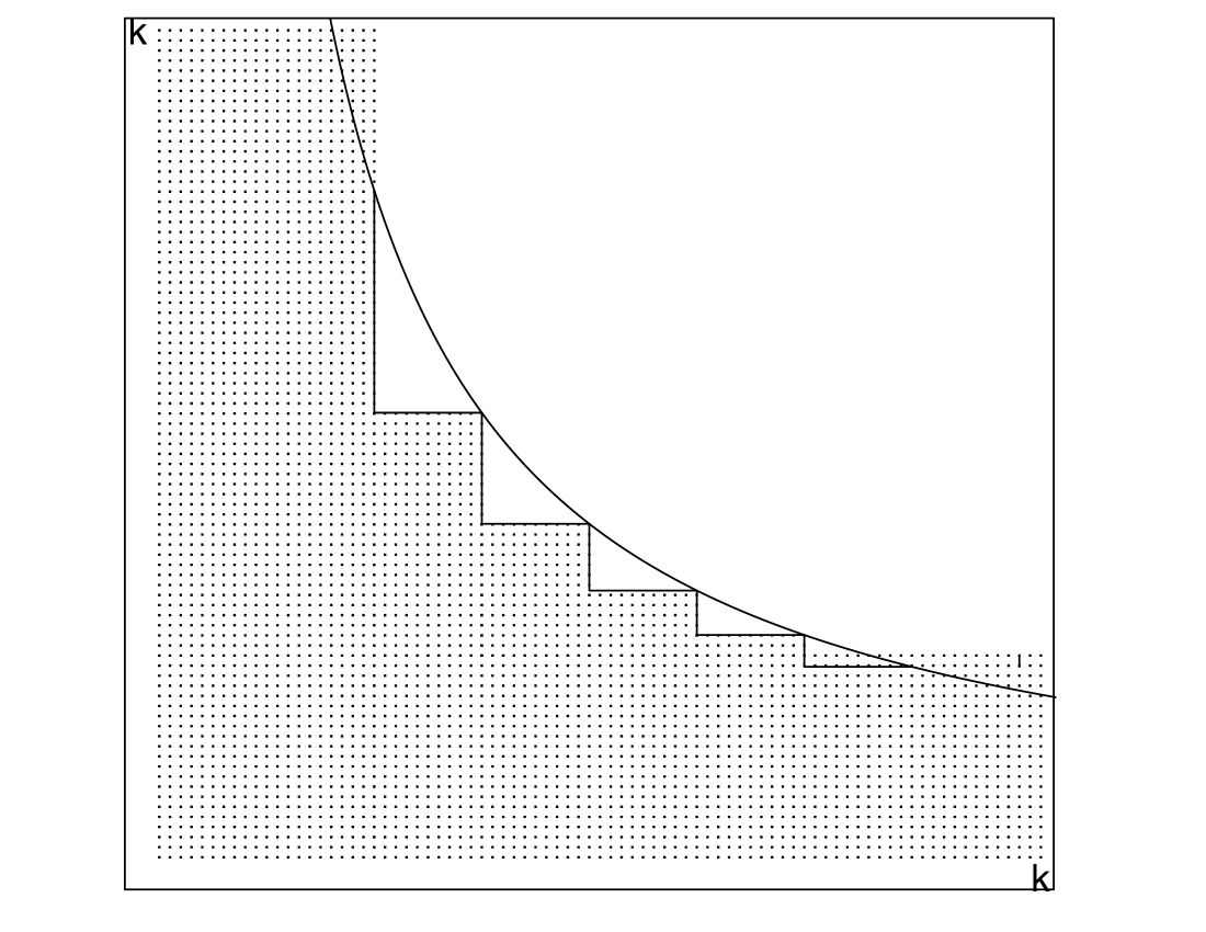
Figure 1: Both axis carry the indices of the basis functions spanning the projection space $L$, and point in the plane refers to a product of two projections. Products of projections on pairs of basis functions in the shaded area are included in the third order influence function. The step function refers to the partitions of the indices as in (9.2).

Before deriving an optimal value of $D$, we introduce the $m$th order estimator for general $m\geq 3$. Again we take the estimator of Theorem 8.1 as starting point, but modify the higher order influence functions $\widetilde{\chi}^{(j)}_{p}$, for $j=4,\ldots,m$, similar and in addition to the modification of the third order influence function. For given $j$ the former influence function is given in Theorem 7.2 (with $m$ of the theorem taken equal to $j$), and is based on a product of $j-1$ projection kernels. We modify this in two steps. For each of the $j-2$ contiguous pairs of kernels ($(1st,2nd),(2nd,3rd),\ldots,((j-2)th,(j-1)th)$) we form a new kernel by truncating the pair at the hyperbola as described previously for the third order kernel, and truncating all other kernels at $n$. Next the modified $j$th order kernel is the sum of the resulting $j-2$ kernels. More formally, the modified $j$th order kernel is equal to

$$\chi_{p}^{(j)}(X_{1},\ldots,X_{j})=\sum_{i=1}^{j-2}\chi_{p}^{(j,i)}(X_{1},\ldots,X_{j}),$$ (9.6)

where $\chi_{p}^{(j,i)}(X_{1},\ldots,X_{j})$ is the symmetrized, degenerate (relative to $L_{2}(p)$) part of the variable, for $i=1,\ldots,j-2$, written in the notation of Theorem 8.1,

$$j!(-1)^{j-1}\,\widetilde{Y}_{1}\Pi_{1,2}^{(0,n]}\underline{A}_{2}\times\cdots\times\underline{A}_{i-1}\Pi_{i-1,i}^{(0,n]}\underline{A}_{i}\times$$

$$\times\Bigl{[}\mathop{\mathchar 4944\relax\mathchar 4944\relax}\limits_{{(r,s):r+s\leq D}\atop{\vee r=0\vee s=0}}\Pi_{i,i+1}^{(k_{r-1},k_{r}]}\underline{A}_{i+1}\Pi_{i+1,i+2}^{{(l_{s-1},l_{s}]}}\Bigr{]}\underline{A}_{i+2}\Pi_{i+2,i+3}^{(0,n]}\times\cdots\times\underline{A}_{j-1}\Pi_{j-1,j}^{(0,n]}\widetilde{A}_{j}.$$

For $j=3$ there is only one pair of kernels, and the construction reduces to the modification (9.3) as discussed previously.

We assume that the projections $\Pi_{p}^{(0,l]}$ and $\Pi_{\hat{p}}^{(0,l]}$ map $L_{s}\bigl{(}\underline{a}\underline{b}g)$ to $L_{s}\bigl{(}\underline{a}\underline{b}g)$, for every $s\in\bigl{[}r/(r-1),r\bigr{]}$, with uniformly bounded norms.

Theorem 9.1.

The estimator (9.1) for $m\geq 3$ with the influence functions $\widetilde{\chi}_{p}^{(j)}$ and $\chi_{p}^{(j)}$ given in (7.5) and (7.7) for $j=1,2$, respectively, and in (9.6) for $j\geq 3$, and with $\Pi_{p}^{(0,l]}$ kernels of orthogonal projections in $L_{2}\bigl{(}\underline{a}\underline{b}g)$ satisfying (13.1) with $\sup_{x}\Pi_{\hat{p}}^{(0,l]}(x,x)\lesssim l$, satisfies, for $r\geq 2$ (and $r/(r-2)=\infty$ if $r=2$),

$$\hat{\mathord{\rm E}}_{p} \hat{\chi}_{n}-\chi(p)=O\Bigl{(}\|\hat{a}-a\|_{r}\|\hat{b}-b\|_{r}\|\hat{g}-g\|_{\frac{mr}{r-2}}^{m-1}\Bigr{)}$$

$$+O\Bigl{(}\Bigl{\|}(I-\Pi_{p}^{(0,k]})\frac{\hat{a}-a}{\underline{a}}\Bigr{\|}_{2}\Bigl{\|}(I-\Pi_{p}^{(0,k]})\frac{\hat{b}-b}{\underline{b}}\Bigr{\|}_{2}\Bigr{)},$$

$$+O\Bigl{(}\sum_{r=1}^{R}\Bigl{\|}(I-\Pi_{\hat{p}}^{(0,k_{r-1}]})\Bigl{(}\frac{\hat{a}-a}{\underline{a}}\Bigr{)}\Bigr{\|}_{r}\Bigl{\|}(I-\Pi_{\hat{p}}^{(0,l_{D-r}]})\Bigl{(}\frac{\hat{b}-b}{\underline{b}}\Bigr{)}\Bigr{\|}_{r}\|\hat{g}-g\|_{\frac{r}{r-2}}\Bigr{)}$$

$$+O\Bigl{(}R\Bigl{\|}(I-\Pi_{\hat{p}}^{(0,n]})\frac{\hat{a}-a}{\underline{a}}\Bigr{\|}_{r}\Bigl{\|}(I-\Pi_{\hat{p}}^{(0,n]})\frac{\hat{b}-b}{\underline{b}}\Bigr{\|}_{r}\|\hat{g}-g\|_{\frac{mr}{r-2}}^{2}\Bigr{)},$$

$$\hat{\mathop{\rm var}}\nolimits_{p}\hat{\chi}_{n}\lesssim\frac{1+R^{2}{\varepsilon}_{n}^{4}}{n}+\frac{k(1+R{\varepsilon}_{n}^{2})}{n^{2}}+\frac{D2^{(\frac{1}{{\alpha}}\vee\frac{1}{{\beta}})D}}{n}.$$

Here ${\varepsilon}_{n}$ is the maximum of the three rates $\|a-\hat{a}\|_{4}$, $\|b-\hat{b}\|_{4}$ and $\|g-\hat{g}\|_{\infty}$ and the constant $c$ depends on the supremum norms of $\underline{a},\underline{b},1/a,b,p/\hat{p},g/\hat{g}$, the norms of the operators $\Pi_{\hat{p}}^{(0,l]}:L_{s}(\underline{a}\underline{b}\hat{g})\to L_{s}(\underline{a}\underline{b}\hat{g})$, for $l=1,\ldots,k$ only, and $r\geq 2$,

A proof of the theorem is presented in Sections 10.3 and 10.4.

The first two terms in the bias are the same as in Theorem 8.1; the third and fourth terms are the price paid for cutting out terms from the influence function. The benefit is a reduced variance. We shall show that the boundary parameter $D$ can be chosen such that the third term in the variance (resulting from the third and higher order parabolic parts of the influence function) is not bigger than the second term, while the increase in bias is negligible. The number $R$ will be logarithmic and ${\varepsilon}_{n}$ a negative power of $n$, the product $R{\varepsilon}_{n}^{2}$ will tend to zero and the first two terms of the variance will be of order $1/n$ and $k/n^{2}$.

Assume that the functions $a$ and $b$ and their estimates are known to belong to models that are well approximated by the base functions $e_{1},e_{2},\ldots$ in the sense that, for $p\in\{p,\hat{p}\}$, and every value $l$ in one of the two grids (9.4)-(9.5),

$$\Bigl{\|}(I-\Pi_{p}^{(0,l]})\Bigl{(}\frac{\hat{a}-a}{\underline{a}}\Bigr{)}\Bigr{\|}_{r} \lesssim\Bigl{(}\frac{1}{l}\Bigr{)}^{{\alpha}/d},$$ (9.7)

$$\Bigl{\|}(I-\Pi_{p}^{(0,l]})\Bigl{(}\frac{\hat{b}-b}{\underline{b}}\Bigr{)}\Bigr{\|}_{r} \lesssim\Bigl{(}\frac{1}{l}\Bigr{)}^{{\beta}/d}.$$ (9.8)

Then the second term in the bias is of the order $(1/k)^{{\alpha}/d+{\beta}/d}$, as in Theorem 8.1, which is smaller than the minimax rate $n^{-(2{\alpha}+2{\beta})/(2{\alpha}+2{\beta}+d)}$ for

$$k\sim n^{2d/(2{\alpha}+2{\beta}+d)}.$$ (9.9)

With this choice of $k$, the upper bound on the variance is of the square minimax rate $n^{-(4{\alpha}+4{\beta})/(2{\alpha}+2{\beta}+d)}$ if $D$ is chosen to satisfy

$$2^{(\frac{1}{{\alpha}}\vee\frac{1}{{\beta}})D}\sim\frac{1}{\log n}n^{(d-2{\alpha}-2{\beta})/(d+2{\alpha}+2{\beta})}.$$ (9.10)

Furthermore, under (9.9) the numbers $R,S$ of grid points are of the order $\log n$.

In the third term of the bias we apply assumptions (9.7)-(9.8) and the identity $k_{r-1}^{\alpha}l_{D-r}^{\beta}\sim n^{{\alpha}+{\beta}}2^{D}$, which results from (9.4)-(9.5), to see that the third term of the bias is of order

$$\sum_{r=1}^{R}\Bigl{(}\frac{1}{k_{r-1}}\Bigr{)}^{{\alpha}/d}\Bigl{(}\frac{1}{l_{D-r}}\Bigr{)}^{{\beta}/d}\|\hat{g}-g\|_{r/(r-2)}\leq R\Bigl{(}\frac{1}{n^{{\alpha}+{\beta}}2^{D}}\Bigr{)}^{1/d}\|\hat{g}-g\|_{r/(r-2)}.$$

If the convergence rate of $\hat{g}$ is $n^{-{\gamma}/(2{\gamma}+d)}$, then, for the choice of $D$ given in (9.10), this can (by a calculation) seen to be of smaller order than the minimax rate $n^{-(2{\alpha}+2{\beta})/(2{\alpha}+2{\beta}+d)}$ if ${\gamma}$ is large enough that

$$\frac{{\gamma}}{2{\gamma}+d}>\Bigl{(}\frac{{\alpha}\vee{\beta}}{d}\Bigr{)}\Bigl{(}\frac{d-2{\alpha}-2{\beta}}{d+2{\alpha}+2{\beta}}\Bigr{)}.$$ (9.11)

The fourth term in the bias can by a similar analysis be seen to be of the order

$$R\Bigl{(}\frac{1}{n}\Bigr{)}^{{\alpha}/d}\Bigl{(}\frac{1}{n}\Bigr{)}^{{\beta}/d}\|\hat{g}-g\|_{(m-2)r/(r-2)}^{2}.$$

Again this is smaller than the minimax rate if ${\gamma}$ satisfies assumption (9.11).

Finally, if the convergence rates of $\hat{a}$ and $\hat{b}$ are $n^{-{\alpha}/(2{\alpha}+d)}$ and $n^{-{\beta}/(2{\beta}+d)}$, then the first term in the upper bound of the bias is of the order

$$\Bigl{(}\frac{1}{n}\Bigr{)}^{{\alpha}/(2{\alpha}+d)+{\beta}/(2{\beta}+d)+(m-1){\gamma}/(2{\gamma}+d)}.$$

We choose $m$ large enough so that this is of smaller order than the preceding terms. In particular, we can choose it so that this is smaller than the minimax rate.

We summarize this in the following corollary, which is the most advanced result of the paper.

Corollary 9.1.

If (9.7)–(9.11) hold, and $\Pi_{p}^{(0,l]}$ are kernels of orthogonal projections in $L_{2}\bigl{(}\underline{a}\underline{b}g)$ satisfying (13.1) with $\sup_{x}\Pi_{\hat{p}}^{(0,l]}(x,x)\leq l$, then the $m$th order estimator with the kernels (9.6) for $j\geq 3$ and sufficiently large $m$ and suitable initial estimators, attains the rate $n^{-(2{\alpha}+2{\beta})/(2{\alpha}+2{\beta}+d)}$ for estimating $\chi(p)$.

10 Proofs

10.1 Proof of Theorem 6.1

Write $\hat{\Pi}$ and $\Pi$ for $\Pi_{\hat{p}}$ and $\Pi_{p}$, respectively, for both the kernels and the corresponding projection operators, and drop $p$ also in $\hat{\mathord{\rm E}}_{p}$ and $\hat{\mathop{\rm var}}\nolimits_{p}$. From (5) and (6.3) we have

$$\hat{\mathord{\rm E}}\hat{\chi}_{n}-\chi(p)$$

$$\quad=-\int(\hat{a}-a)(\hat{b}-b)\,g\,d{\nu}-\hat{\mathord{\rm E}}A_{1}\bigl{(}Y_{1}-\hat{b}(Z_{1})\bigr{)}\bigl{(}A_{2}\hat{a}(Z_{2})-1\bigr{)}\hat{\Pi}(Z_{1},Z_{2})$$

$$\quad=-\int(\hat{a}-a)(\hat{b}-b)\,g\,d{\nu}+\int\!\!\int\bigl{[}(\hat{a}-a)\times(\hat{b}-b)\bigr{]}\,\bigl{(}g\times g\bigr{)}\,\hat{\Pi}\,d{\nu}\times{\nu}.$$

The double integral on the far right with $\hat{\Pi}$ replaced by $\Pi$ can be written as the single integral $\int(\hat{a}-a)\Pi(\hat{b}-b)\,g\,d{\nu}$, for $\Pi(\hat{b}-b)$ the image of $\hat{b}-b$ under the projection $\Pi$. Added to the first integral on the right this gives $-\int(\hat{a}-a)(I-\Pi)(\hat{b}-b)\,g\,d{\nu}$, which is bounded in absolute value by the second term in the upper bound for the bias.

Replacement of $\hat{\Pi}$ by $\Pi$ in the double integral gives a difference

$$\int\!\!\int\bigl{[}(\hat{a}-a)\times(\hat{b}-b)\bigr{]}\,g\times g\,(\hat{\Pi}-\Pi)\,d{\nu}\times{\nu}$$

$$\hskip 40.00006pt=\int(\hat{a}-a)\left(\hat{\Pi}\Bigl{(}(\hat{b}-b)\frac{g}{\hat{g}}\Bigr{)}-\Pi(\hat{b}-b)\right)\,g\,d{\nu}$$

$$\hskip 40.00006pt\leq\|\hat{a}-a\|_{s}\left\|\hat{\Pi}\Bigl{(}(\hat{b}-b)\frac{g}{\hat{g}}\Bigr{)}-\Pi(\hat{b}-b)\right\|_{r,\hat{g}}\|g/\hat{g}\|_{\infty}^{1/r},$$

by Hölder’s inequality, for a conjugate pair $(r,s)$. Considering $\hat{\Pi}$ as the projection in $L_{2}(\hat{g})$ with weight 1, and $\Pi$ as the weighted projection in $L_{2}(\hat{g})$ with weight function $\hat{w}=g/\hat{g}$, we can apply Lemma 13.7(i) (with $q=s/r$ and $rp=s/(s-2)$) to see that this is bounded in absolute value by

$$\|\hat{a}-a\|_{s}\|\hat{\Pi}\|_{s,\hat{g}}\|\Pi\|_{s,\hat{g}}\|\hat{b}-b\|_{s,\hat{g}}\|\hat{w}-1\|_{s/(s-2),\hat{g}}\|w\|_{\infty}^{1/r}.$$

Because $\hat{w}$ is assumed bounded away from 0 and infinity, this is of the same order as the first term in the upper bound on the bias (if $r$ replaces $s$).

Because the function $\chi_{\hat{p}}^{(1)}$ is uniformly bounded, the (conditional) variance of $\mathbb{U}_{n}\chi_{\hat{p}}^{(1)}$ is of the order $O(1/n)$. Thus for the variance bound it suffices to consider the (conditional) variance of $\mathbb{U}_{n}\chi_{\hat{p}}^{(2)}$. In view of Lemma 14.1 this is bounded above by a multiple of

$$\frac{1}{n^{2}}P^{2}(\chi_{\hat{p}}^{(2)})^{2}+\max_{i\in\{1,2\}}\frac{1}{n}P\Bigl{(}\mathord{\rm E}\bigl{(}\chi_{\hat{p}}^{(2)}\mathchar 25194\relax X_{i}\bigr{)}\Bigr{)}^{2}.$$

The variables $A\bigl{(}Y-\hat{b}(Z)\bigr{)}$ and $\bigl{(}A\hat{a}(Z)-1\bigr{)}$ are uniformly bounded. Hence the first term is bounded above by a multiple of $n^{-2}\int\hat{\Pi}^{2}\,(\hat{g}\times\hat{g})\,d{\nu}\times{\nu}$, which is equal to $k/n^{2}$, by Lemma 13.3. The conditional expectations in the second term can be written $A_{1}\bigl{(}Y_{1}-\hat{b}(Z_{1})\bigr{)}\Pi_{\hat{p}}\bigl{(}\hat{a}/a-1)g/\hat{g}\bigr{)}(Z_{1})$ and $\Pi_{\hat{p}}\bigl{(}\hat{b}-b)g/\hat{g}\bigr{)}(Z_{2})(A_{2}\hat{a}(Z_{2})-1)$, for $i=1$ and $i=2$, respectively, where $\Pi_{p}$ is the operator defined by the kernel. Because the second moments of these variables under $\hat{p}$ are uniformly bounded, the second term contributes a factor of order $1/n$ only.

10.2 Proof of Theorems 8.1 and 8.2

Let $\hat{A}$ and $\hat{Y}$ be $\widetilde{A}$ and $\widetilde{Y}$ as in (7.6) with $a$ and $b$ in their definitions replaced by $\hat{a}$ and $\hat{b}$. Because $\hat{a}$ and $\hat{b}$ are projected onto themselves under the map $(a,b,g)\mapsto(\widetilde{a},\widetilde{b},g)$ (see Theorem 7.1), we actually obtain the same variables by replacing $\widetilde{a}$ and $\widetilde{b}$ by $\hat{a}$ and $\hat{b}$, respectively: $\hat{A}=\bigl{(}A\hat{a}(Z)-1\bigr{)}\underline{b}(Z)$ and $\hat{Y}=A\bigl{(}Y-\hat{b}(Z)\bigr{)}\underline{a}(Z)$. Furthermore, let $\Pi$ and $\hat{\Pi}$ denote the operators $\Pi_{p}$ and $\Pi_{\hat{p}}$, respectively, and $\Pi_{i,j}$ and $\hat{\Pi}_{i,j}$ their kernels evaluated at $(Z_{i},Z_{j})$.

By explicit calculations,

$$\chi(\hat{p})+\hat{\mathord{\rm E}}_{p}\widetilde{\chi}_{\hat{p}}^{(1)}-\chi(p)=-\int(\hat{a}-a)(\hat{b}-b)\,g\,d{\nu}=\hat{\mathord{\rm E}}\hat{A}_{1}\Pi_{1,2}\hat{Y}_{2}-\hat{R},$$ (10.1)

for $\hat{R}$ defined by

$$\hat{R}=\int\Bigl{(}\frac{\hat{a}-a}{\underline{a}}\Bigr{)}(I-\Pi)\Bigl{(}\frac{\hat{b}-b}{\underline{b}}\Bigr{)}\underline{a}\underline{b}g\,d{\nu}.$$

The variable $\hat{R}$ is bounded by the second term in the expression for $\hat{\mathord{\rm E}}_{p}\hat{\chi}_{n}-\chi(p)$ in the statement of the theorem. We next show by induction on $m$ that

$$\qquad\hskip 40.00006pt\hskip 40.00006pt\hat{R}+\chi(\hat{p})+\hat{\mathord{\rm E}}\widetilde{\chi}_{\hat{p}}^{(1)}+\cdots+\frac{1}{m!}\hat{\mathord{\rm E}}\widetilde{\chi}_{\hat{p}}^{(m)}-\chi(p)$$ (10.2)

$$=(-1)^{m-1}\hat{\mathord{\rm E}}\hat{A}_{1}(\hat{\Pi}-\Pi)_{1,2}\underline{A}_{2}(\hat{\Pi}-\Pi)_{2,3}\times\cdots\times\underline{A}_{m-1}(\hat{\Pi}-\Pi)_{m-1,m}\hat{Y}_{m}.$$

The analysis of the bias can then be concluded by showing that the right side of (10.2) is of the order as the first term given in the theorem.

Equation (10.1) and the definition of $\widetilde{\chi}_{p}^{(2)}$ readily show that identity (10.2) is true for $m=2$. We proceed to general $m$ by induction. Relative to its value for $m$ the left side receives for $(m+1)$ the extra term $\hat{\mathord{\rm E}}\chi_{\hat{p}}^{(m+1)}/(m+1)!$, which is equal to $(-1)^{m}$ times $\hat{\mathord{\rm E}}\hat{A}_{1}\hat{\Pi}_{1,2}\underline{A}_{2}\hat{\Pi}_{2,3}\times\cdots\times\underline{A}_{m}\hat{\Pi}_{m,m+1}\hat{Y}_{m+1}$ minus a sum of terms resulting from projections of this leading term. This extra term without the factor $(-1)^{m}$ (but including the projections) can be written (cf. (7.7) and (2.1))

$$\sum_{i=0}^{m-1}{m-1\choose i}\hat{\mathord{\rm E}}\hat{A}_{1}\hat{\Pi}_{1,2}\underline{A}_{2}\hat{\Pi}_{2,3}\times\cdots\times\underline{A}_{m-i}\hat{\Pi}_{m-i,m-i+1}\hat{Y}_{m-i+1}(-1)^{i}.$$ (10.3)

To prove the induction hypothesis for $m+1$ it suffices to show that this is equal to

$$\hat{\mathord{\rm E}}\hat{A}_{1}(\hat{\Pi}-\Pi)_{1,2}\underline{A}_{2}(\hat{\Pi}-\Pi)_{2,3}\times\cdots\times\underline{A}_{m-1}(\hat{\Pi}-\Pi)_{m-1,m}\hat{Y}_{m}$$

$$\qquad+\hat{\mathord{\rm E}}\hat{A}_{1}(\hat{\Pi}-\Pi)_{1,2}\underline{A}_{2}(\hat{\Pi}-\Pi)_{2,3}\times\cdots\times\underline{A}_{m}(\hat{\Pi}-\Pi)_{m,m+1}\hat{Y}_{m+1}.$$ (10.4)

To achieve this we expand the two terms of the preceding display into sums of expressions of the form, with each $K_{j,j+1}^{(j)}$ equal to $\hat{\Pi}_{j,j+1}$ or $\Pi_{j,j+1}$ and $l$ the number of $j$ for which the first alternative is true,

$$B_{l}:=(-1)^{m-1-l}\,\hat{\mathord{\rm E}}\hat{A}_{1}K_{1,2}^{(1)}\underline{A}_{2}K_{2,3}^{(2)}\times\cdots\times\underline{A}_{m-1}K_{m-1,m}^{(m-1)}\hat{Y}_{m},$$ (10.5)

and of the same form with $m+1$ replacing $m$ for the second term of (10.4). As the notation suggests the expression in (10.5) depends on $l$ (and $m$, but this is fixed), but not on which $K$ are equal to $\hat{\Pi}$ or $\Pi$. To see this we use that $\Pi$ is a projection onto $L$ in $L_{2}(\underline{a}\underline{b}g)$, so that $\int\Pi_{1,2}\,{\gamma}(z_{2})\,(\underline{a}\underline{b}g)(z_{2})\,d{\nu}(z_{2})={\gamma}(z_{1})$ for every ${\gamma}\in L$; and $\hat{\Pi}$ is also a projection onto $L$, so that as a function of one argument $\hat{\Pi}_{1,2}$ is contained in $L$. This observation yields the identities, for $K$ equal to $\hat{\Pi}$ or $\Pi$,

$$\hat{\mathord{\rm E}}_{Z_{j}}\Pi_{j-1,j}\underline{A}_{j}K_{j,j+1}=K_{j-1,j+1}=\hat{\mathord{\rm E}}_{Z_{j}}K_{j-1,j}\underline{A}_{j}\Pi_{j,j+1}.$$

This allows to reduce (10.5) to

$$B_{l} =(-1)^{m-1-l}\,\hat{\mathord{\rm E}}\hat{A}_{1}\hat{\Pi}_{1,2}\underline{A}_{2}\hat{\Pi}_{2,3}\times\cdots\times\underline{A}_{l}\hat{\Pi}_{l,l+1}\hat{Y}_{l+1},\qquad l\geq 1,$$

$$B_{0} =(-1)^{m-1}\hat{\mathord{\rm E}}\hat{A}_{1}\Pi_{1,2}\hat{Y}_{2}.$$

Thus after expanding the two terms of (10.4) in the quantities $B_{l}$, and simplifying these quantities, we can write their sum (10.4)

$$(B_{0}-B_{0})+\sum_{l=1}^{m-1}\left({m\choose l}-{m-1\choose l}\right)B_{l}(-1)^{m-l}+B_{m}.$$

The difference of the binomial coefficients is ${m-1\choose l-1}$. The expression is equal to (10.3), as claimed. This completes the proof of (10.2).

Next we bound the right side of (10.2), by taking the expectation in turn with respect to $X_{m},X_{m-1},\ldots,X_{1}$. For $M_{\hat{w}}$ multiplication by the function $\hat{w}=g/\hat{g}$,

$$\hat{\mathord{\rm E}}_{X_{m}}(\hat{\Pi}-\Pi)_{m-1,m}\hat{Y}_{m}=(\hat{\Pi}M_{\hat{w}}-\Pi)\Bigl{(}\frac{\hat{b}-b}{\underline{b}}\Bigr{)}(Z_{m-1}).$$

Next, for any function $h$ and $i=m-1,m-2,\ldots,2$,

$$\hat{\mathord{\rm E}}_{X_{i}}(\hat{\Pi}-\Pi)_{i-1,i}\underline{A}_{i}h(Z_{i})=(\hat{\Pi}M_{\hat{w}}-\Pi)h(Z_{i-1}).$$

Combining these equations, we can write the right side of (10.2) in the form

$$(-1)^{m-1}\int\Bigl{(}\frac{a-\hat{a}}{\underline{a}}\Bigr{)}\biggl{[}\bigl{(}\hat{\Pi}M_{\hat{w}}-\Pi\bigr{)}^{m-1}\Bigl{(}\frac{\hat{b}-b}{\underline{b}}\Bigr{)}\biggr{]}\,\underline{a}\underline{b}g\,d{\nu}.$$

We bound this by first applying Hölder’s inequality, with conjugate pair $({\tau},t)$ with ${\tau}$ equal to $r$ as in the statement of the theorem, and next Lemma 13.7(iii), with $\hat{\Pi}$ and $\Pi$ viewed as weighted orthogonal projections in $L_{2}(\underline{a}\underline{b}\hat{g})$ with weights 1 and $\hat{w}$, respectively, and $r={\tau}(m-1)/(m+{\tau}-3)$, $p=(m+{\tau}-3)/({\tau}-2)$ and $q=(m+{\tau}-3)/(m-1)$, so that $rp=(m-1){\tau}/({\tau}-2)$ and $rq={\tau}$ (and $m$ of the lemma taken equal to the present $m$ minus 1).

By Lemma 14.1 the (conditional) variance of $(j!)^{-1}\mathbb{U}_{n}\chi_{\hat{p}}^{(j)}$ is bounded above by

$$\sum_{l=1}^{j}\frac{2^{j}j^{2l}}{n^{l}}\mathord{\rm E}_{p}\biggl{(}\mathord{\rm E}_{p}\Bigl{(}S_{j}D_{\hat{p}}\bigl{[}\hat{A}_{1}\hat{\Pi}_{1,2}\underline{A}_{2}\hat{\Pi}_{2,3}\cdots\hat{\Pi}_{j-1,j}\hat{Y}_{j}\bigr{]}\mathchar 25194\relax X_{1},\ldots,X_{l}\Bigr{)}\biggr{)}^{2}.$$

Here $\hat{\Pi}_{i,j}$ are the estimated kernels (the original ones with $p$ replaced by $\hat{p}$) and $D_{\hat{p}}$ is the operation of making degenerate under $\hat{p}$ (not under $p$!).

By Lemma 14.2(ii), for any function $h(X_{1},\ldots,X_{j})$ the second moment of $\mathord{\rm E}\bigl{(}S_{j}h(X_{1},\ldots,X_{j})\mathchar 25194\relax X_{1},\ldots,X_{l}\bigr{)}=(j!)^{-1}\sum_{\sigma}\mathord{\rm E}\bigl{(}h(X_{{\sigma}(1)},\ldots,X_{{\sigma}(j)})\mathchar 25194\relax X_{1},\ldots,X_{l}\bigr{)}$ is bounded above by the maximum over all permutations ${\sigma}$ of the second moments of the variables $\mathord{\rm E}\bigl{(}h(X_{{\sigma}(1)},\ldots,X_{{\sigma}(j)})\mathchar 25194\relax X_{1},\ldots,X_{l}\bigr{)}$. Because $X_{1},\ldots,X_{j}$ are i.i.d., we can move the permutation ${\sigma}$ from the argument of $h$ to the conditioning variables, and conclude that the second moment in the $l$th term on the right side is bounded above by

$$\max_{{B\subset\{1,\ldots,j\}:}\atop{|B|=l}}\mathord{\rm E}_{p}\biggl{(}\mathord{\rm E}_{p}\Bigl{(}D_{\hat{p}}\bigl{[}\hat{A}_{1}\hat{\Pi}_{1,2}\underline{A}_{2}\hat{\Pi}_{2,3}\cdots\underline{A}_{j-1}\hat{\Pi}_{j-1,j}\hat{Y}_{j}\bigr{]}\mathchar 25194\relax X_{B}\Bigr{)}\biggr{)}^{2}.$$

These are bounded in Lemma 10.2.

We complete the proof of Theorem 8.1 by bounding the square of $\hat{\chi}_{n}-\mathord{\rm E}_{p}\hat{\chi}_{n}$ by $\sum_{j=1}^{m}2^{j}\bigl{(}(\mathbb{U}_{n}-P^{n})\widetilde{\chi}_{\hat{p}}^{(j)}/j!\bigr{)}^{2}\sum_{j}2^{-j}$. The extra factor $2^{j}$ can be incorporated in the constant $c$ in the theorem. We finish by changing the order of summation in the double sum $\sum_{j=2}^{m}\sum_{l=1}^{j}$, so as to collect the terms by the order of $k^{l-1}/n^{l}$.

For the proof of Theorem 8.2 it clearly suffices to show that

$$\hat{\mathord{\rm E}}_{p}\sqrt{n}\bigl{(}\hat{\chi}_{n}-\chi(p)-\mathbb{P}_{n}\widetilde{\chi}_{p}^{(1)}\bigr{)} \ {\mathchoice{\raise-1.5pt\hbox{$\buildrel\small P\over{\rightarrow}$}}{\raise-2.0pt\hbox{$\buildrel\small P\over{\rightarrow}$}}{}{}}\ 0,$$

$$\hat{\mathop{\rm var}}\nolimits_{p}\sqrt{n}\bigl{(}\hat{\chi}_{n}-\chi(p)-\mathbb{P}_{n}\widetilde{\chi}_{p}^{(1)}\bigr{)} \ {\mathchoice{\raise-1.5pt\hbox{$\buildrel\small P\over{\rightarrow}$}}{\raise-2.0pt\hbox{$\buildrel\small P\over{\rightarrow}$}}{}{}}\ 0.$$

Because an influence function is centered at mean zero, the first is simply $\sqrt{n}$ times the bias of $\hat{\chi}_{n}$. By Theorem 8.1 the bias is of the order

$$\Bigl{(}\frac{\log n}{n}\Bigr{)}^{{\alpha}/(2{\alpha}+d)+{\beta}/(2{\beta}+d)+{\gamma}(m-1)/(2{\gamma}+d)}+\Bigl{(}\frac{1}{k}\Bigr{)}^{({\alpha}+{\beta})/d}.$$

The first term is trivially $o(n^{-1/2})$, as $m_{n}\rightarrow\infty$. In the second we write $({\alpha}+{\beta})/d=r/2$, where $r>1$ by assumption, and see that it is $o(n^{-1/2})$, since $kn^{-1/r}\rightarrow\infty$.

To handle the variance we split the estimator $\hat{\chi}_{n}$ in its linear and higher order terms. By Lemma 14.2(i) and the argument given previously, for $c$ a sufficiently large constant, the variance of the higher order terms satisfies

$$\mathop{\rm var}\nolimits\sum_{j=2}^{m}\frac{1}{j!}\mathbb{U}_{n}\widetilde{\chi}_{\hat{p}}^{(j)}\leq\sum_{j=2}^{m}\sum_{l=1}^{j}\frac{c^{j}j^{2l}}{n^{l}}k^{l-1}{\varepsilon}_{n}^{2(j-l)}$$

$$\qquad=\sum_{j=2}^{m}\frac{j^{2}{\varepsilon}_{n}^{2j}c^{j}}{n{\varepsilon}_{n}^{2}}\sum_{l=1}^{j}\Bigl{(}\frac{j^{2}k}{n{\varepsilon}_{n}^{2}}\Bigr{)}^{l-1}=\sum_{j=2}^{m}\frac{j^{2}{\varepsilon}_{n}^{2j}c^{j}}{n{\varepsilon}_{n}^{2}}\frac{(\bigl{(}j^{2}k/(n{\varepsilon}_{n}^{2})\bigr{)}^{j}-1}{j^{2}k/(n{\varepsilon}_{n}^{2})-1}.$$

By assumption ${\varepsilon}_{n}=O(n^{-{\eta}})$ for some ${\eta}>0$ and $k\sim n/(\log n)^{3}$. Thus $j^{2}k/(n{\varepsilon}_{n}^{2})\rightarrow\infty$ uniformly in $j\geq 1$, and the preceding display is bounded above by

$$2\sum_{j=2}^{m}\frac{j^{2}{\varepsilon}_{n}^{2j}c^{j}}{n{\varepsilon}_{n}^{2}}\Bigl{(}\frac{j^{2}k}{n{\varepsilon}_{n}^{2}}\Bigr{)}^{j-1}\lesssim\frac{1}{n}\sum_{j=2}^{m}\Bigl{(}\frac{2cj^{2}k}{n}\Bigr{)}^{j-1}\lesssim\frac{1}{n}\sum_{j=2}^{\infty}\Bigl{(}\frac{1}{\log n}\Bigr{)}^{j-1}\lesssim\frac{1}{n\log n},$$

since $j^{2}\lesssim 2^{j-1}$ and $2cj^{2}k/n\leq 2cm^{2}k/n\leq 1/\log n$, for every $j\leq m$. Finally the linear term in $\hat{\chi}_{n}$ gives the contribution

$$\hat{\mathop{\rm var}}\nolimits_{p}\sqrt{n}\bigl{(}\mathbb{P}_{n}\widetilde{\chi}_{\hat{p}}^{(1)}-\chi(p)-\mathbb{P}_{n}\widetilde{\chi}_{p}^{(1)}\bigr{)}=\hat{\mathop{\rm var}}\nolimits(\widetilde{\chi}^{(1)}_{\hat{p}}-\widetilde{\chi}^{(1)}_{p}).$$

From the explicit expression (4.7) for the first order influence function (or (7.5) in the case of $\hat{p}$, which gives an identical function), this is seen to tend to zero by the dominated convergence theorem.

10.3 Proof of Theorem 9.1 for $m=3$

The theorem asserts that the bias of the estimator $\hat{\chi}_{n}$ is equal to the sum of four terms, the first two of which also arise in the bias of the estimator considered in Theorem 8.1. Therefore, we can prove the assertion on the bias by showing that the expected values of the current estimator $\hat{\chi}_{n}$ (for $m=3$) and the estimator in Theorem 8.1 differ by less than the additional bias terms in Theorem 9.1.

The two estimators differ only in their third order influence functions, where the present estimator retains only the terms in the double sum (9.3) with $r=0$, $s=0$, or $r+s\leq D$. Thus the difference of the expectations of the two estimators is equal to

$$\mathop{\mathchar 4944\relax\mathchar 4944\relax}\limits_{{r+s>D}\atop{r,s\geq 1}}\hat{\mathord{\rm E}}_{p}\hat{A}_{1}\Bigl{[}\hat{\Pi}^{(k_{r-1},k_{r}]}(Z_{1},Z_{2})\underline{A}_{2} \hat{\Pi}^{(l_{s-1},l_{s}]}(Z_{2},Z_{3})$$

$$-\hat{\Pi}^{(k_{r-1}\vee l_{s-1},k_{r}\wedge l_{s}]}(Z_{1},Z_{3})\Bigr{]}\hat{Y}_{3}.$$

The expectation $\hat{\mathord{\rm E}}_{p}$ refers to the variable $(X_{1},X_{2},X_{3})$ for fixed values of the preliminary samples, which are indicated in the “hat” symbols on $\hat{A}_{1},\hat{Y}_{3}$ and the kernels, and hence is an integral relative to the density $(x_{1},x_{2},x_{3})\mapsto p(x_{1})p(x_{2})p(x_{3})$. If we replace $p(x_{2})$ in this density by $\hat{p}(x_{2})$, then the integral will be zero, as the kernel is degenerate under $\hat{P}$. Thus we may integrate against $(x_{1},x_{2},x_{3})\mapsto p(x_{1})(p-\hat{p})(x_{2})p(x_{3})$. In that case the projection term $\hat{A}_{1}\hat{\Pi}^{(k_{r-1}\vee l_{s-1},k_{r}\wedge l_{s}]}(Z_{1},Z_{3})\hat{Y}_{3}$ integrates to zero, as it does not depend on $X_{2}$ and $\int(p-\hat{p})(x_{2})\,d{\mu}(x_{2})=0$, and hence can be dropped. Next we condition $\hat{A}_{1}$ and $\hat{Y}_{3}$ on $Z_{1},Z_{2},Z_{3}$ and write the preceding display in the form

$$\mathop{\mathchar 4944\relax\mathchar 4944\relax}\limits_{{r+s>D}\atop{r,s\geq 1}}\int\!\!\int\!\!\int\frac{\hat{a}-a}{\underline{a}}(z_{1})\hat{\Pi}^{(k_{r-1},k_{r}]}(z_{1},z_{2}) \hat{\Pi}^{(l_{s-1},l_{s}]}(z_{2},z_{3})\frac{\hat{b}-b}{\underline{b}}(z_{3})$$

$$\times\,d{\rho}(z_{1})\,d({\rho}-\hat{\rho})(z_{2})\,d{\rho}(z_{3}).$$

for ${\rho}$ and $\hat{\rho}$ the measures defined by $d{\rho}=\underline{a}\underline{b}g\,d{\nu}$ and $d\hat{\rho}=\underline{a}\underline{b}\hat{g}\,d{\nu}$. The double sum can be rewritten as the sum over $r$ running from $1$ to $R$ and over $s$ from $D-r+1$ to $S$, which gives the equivalent representation, with the $\times$ referring to “tensor products” as explained in Section 2,

$$\sum_{r=1}^{R}\int\Bigl{(}\frac{\hat{a}-a}{\underline{a}}\times 1\times\frac{\hat{b}-b}{\underline{b}}\Bigr{)}\,\,\Bigl{(}\hat{\Pi}^{(k_{r-1},k_{r}]}\times\hat{\Pi}^{(l_{D-r},k]}\Bigr{)}\,d\bigl{(}{\rho}\times({\rho}-\hat{\rho})\times{\rho}\bigr{)}.$$

We write $\hat{\Pi}^{(k_{r-1},k_{r}]}=\hat{\Pi}^{(k_{r-1},k]}-\hat{\Pi}^{(k_{r},k]}$, and next arrive at the difference of two expressions of the type, with $k_{r}^{\prime}=k_{r-1}$ and $k_{r}^{\prime}=k_{r}$, respectively,

$$\sum_{r=1}^{R}\int\Bigl{(}\frac{\hat{a}-a}{\underline{a}}\times 1\times\frac{\hat{b}-b}{\underline{b}}\Bigr{)}\,\Bigl{(}\hat{\Pi}^{(k_{r}^{\prime},k]}\times\hat{\Pi}^{(l_{D-r},k]}\Bigr{)}\,d\bigl{(}{\rho}\times({\rho}-\hat{\rho})\times{\rho}\bigr{)}.$$

If the measure of integration were $\hat{\rho}\times({\rho}-\hat{\rho})\times\hat{\rho}$ (with $\hat{\rho}$ instead of ${\rho}$), then we could perform the integrals on $z_{1}$ and $z_{3}$ and next apply Hölder’s inequality to bound the resulting expression in absolute value by

$$\sum_{r=1}^{R}\Bigl{\|}\hat{\Pi}^{(k_{r}^{\prime},k]}\Bigl{(}\frac{\hat{a}-a}{\underline{a}}\Bigr{)}\Bigr{\|}_{r}\Bigl{\|}\hat{\Pi}^{(l_{D-r},k]}\Bigl{(}\frac{\hat{b}-b}{\underline{b}}\Bigr{)}\Bigr{\|}_{r}\Big{\|}\frac{g}{\hat{g}}-1\Bigr{\|}_{r/(r-2)},$$

where the norms are those of $L_{2}(\underline{a}\underline{b}\hat{g})$, which are equivalent to those of $L_{2}({\nu})$, by assumption. We can write $\hat{\Pi}^{(l,k]}=\hat{\Pi}^{(0,k]}(I-\hat{\Pi}^{(0,l]})$ and use the assumed boundedness of $\hat{\Pi}^{(0,l]}$ as an operator on $L_{r}(\underline{a}\underline{b}g)$ to bound this by the third term in the bias.

Replacing ${\rho}\times({\rho}-\hat{\rho})\times{\rho}$ by $\hat{\rho}\times({\rho}-\hat{\rho})\times\hat{\rho}$ can be achieved by writing the first and last occurrence of ${\rho}$ as ${\rho}=\hat{\rho}+({\rho}-\hat{\rho})$ and expanding the resulting expression on the $+$ signs into four terms. One of these has the measure $\hat{\rho}\times({\rho}-\hat{\rho})\times\hat{\rho}$. The other three terms have two or three occurrences of ${\rho}-\hat{\rho}$, and can be bounded by the first term in the bias (with $m=3$). This is argued precisely under (10.10) below.

Because the first and second order influence functions are equal to those of the estimator considered in Theorem 8.1, the (conditional) variances of $\mathbb{U}_{n}\widetilde{\chi}_{\hat{p}}^{(j)}$ for $j=1,2$ can be seen to be of the orders $O(1/n)$ and $O(k/n^{2})$, respectively, by the same proof. By Lemma 14.1 the variance for $j=3$ satisfies (see (14.1))

$$\mathop{\rm var}\nolimits\mathbb{U}_{n}\chi_{\hat{p}}^{(3)}\lesssim\sum_{l=1}^{3}\frac{1}{n^{l}}\mathord{\rm E}_{p}\biggl{(}\mathord{\rm E}_{p}\Bigl{(}\widetilde{\chi}_{\hat{p}}^{(3)}(X_{1},X_{2},X_{3})\mathchar 25194\relax X_{1},\ldots,X_{l}\Bigr{)}\biggr{)}^{2}.$$

Here the influence function is given in (9.3) and can also be written

$$\frac{1}{6}\chi_{\hat{p}}^{(3)}(X_{1},X_{2},X_{3}) =\mathop{\mathchar 4944\relax\mathchar 4944\relax}\limits_{{(r,s):r+s\leq D}\atop{\vee r=0\vee s=0}}\!\!S_{3}D_{\hat{p}}\Bigl{[}\hat{A}_{1}\hat{\Pi}_{1,2}^{(k_{r-1},k_{r}]}\underline{A}_{2}\hat{\Pi}_{2,3}^{(l_{s-1},l_{s}]}\hat{Y}_{3}\Bigr{]}$$

$$=\sum_{r=0}^{R}\!\!S_{3}D_{p}\Bigl{[}\hat{A}_{1}\hat{\Pi}_{1,2}^{(k_{r-1},k_{r}]}\underline{A}_{2}\hat{\Pi}_{2,3}^{(0,l_{D-r}^{\prime}]}\hat{Y}_{3}\Bigr{]},$$

where $l_{D-r}^{\prime}=l_{D-r}\vee n$. The degeneracy $D_{\hat{p}}$ operator works on $X_{2}$ only.

In the term for $l=3$ we change measure from $p$ to $\hat{p}$, bound out $\hat{A}_{1}$ and $\hat{Y}_{3}$, and pull out the degeneracy operator to obtain the upper bound a multiple of

$$\frac{1}{n^{3}}\Big{\|}\frac{p}{\hat{p}}\Bigr{\|}_{\infty}^{2}\hat{P}^{3}\Bigl{(}\sum_{r=0}^{R}\hat{\Pi}_{1,2}^{(k_{r-1},k_{r}]}\underline{A}_{2}\hat{\Pi}_{2,3}^{(0,l_{D-r}^{\prime}]}\Bigr{)}^{2}.$$

After bounding out $\hat{A}_{1}^{2}$ and $\hat{Y}_{3}^{2}$, we write the squared sum as a double sum. From the fact that the projections $\hat{\Pi}^{(k_{r-1},k_{r}]}$ are orthogonal for different $r$, it follows that the off-diagonal terms of the double sum vanish (the expectation with respect to $X_{1}$ is zero). Thus the preceding display is bounded above by a multiple of

$$\frac{1}{n^{3}}\sum_{r=0}^{R}\hat{P}^{3}\bigl{(}\hat{\Pi}^{(k_{r-1},k_{r}]}(Z_{1},Z_{2})\underline{A}_{2}\hat{\Pi}^{(0,l_{D-r}^{\prime}]}(Z_{2},Z_{3})\bigr{)}^{2}.$$

By Lemmas 13.4 and 13.3 and the assumption that $\sup_{z}\hat{\Pi}^{(0,l]}(z,z)\lesssim l$ this is bounded by a multiple of

$$\frac{1}{n^{3}}\sum_{r=0}^{R}(k_{r}-k_{r-1})l_{D-r}^{\prime}\leq\frac{1}{n^{3}}\Bigl{(}nk+\sum_{r=1}^{R}(k_{r}-k_{r-1})(l_{D-r}+n)\Bigr{)}.$$

By (9.4) $k_{r}-k_{r-1}=(1-2^{-{\alpha}})k_{r}\lesssim k_{r}=n2^{r/{\alpha}}$ for $r\geq 1$. On substituting this in the display, and noting that $l_{D-r}=0$ if $r>D$, we see that this is bounded by a multiple of $k/n^{2}+2^{D/{\alpha}\vee D/{\beta}}/n$ if ${\alpha}\not={\beta}$ and bounded by a multiple of $k/n^{2}+D2^{D/{\alpha}}/n$ if ${\alpha}={\beta}$.

The second moment in the right side for $l=1$ or $l=2$ is bounded above by a multiple of

$$\max_{{B\subset\{1,2,3\}}\atop{|B|=l}}\mathord{\rm E}_{\hat{p}}\biggl{(}\mathord{\rm E}_{p}\Bigl{(}\mathop{\mathchar 4944\relax\mathchar 4944\relax}\limits_{{(r,s):r+s\leq D}\atop{\vee r=0\vee s=0}}\!\!D_{\hat{p}}\Bigl{[}\hat{A}_{1}\hat{\Pi}_{1,2}^{(k_{r-1},k_{r}]}\underline{A}_{2}\hat{\Pi}_{2,3}^{(l_{s-1},l_{s}]}\hat{Y}_{3}\Bigr{]}\mathchar 25194\relax X_{B}\Bigr{)}\biggr{)}^{2}.$$

We consider the various subsets $B$ separately: $\{1,2\},\{1,3\},\{2,3\},\{1\},\{2\},\{3\}$. Abbreviate $\hat{w}=g/\hat{g}$ and $(\underline{a}\underline{b})(z_{i})\,d\hat{G}(z_{i})=\hat{g}_{i}\,di$.

$B=\{1,2\}$. Taking first the conditional expectation given $Z_{3}$ reduces $\hat{Y}_{3}$ to $(b-\hat{b})/\underline{b}$, and hence

$$\mathord{\rm E}_{p}\biggl{(}\sum_{r=0}^{R}D_{\hat{p}}\Bigl{[}\hat{A}_{1}\hat{\Pi}_{1,2}^{(k_{r-1},k_{r}]}\underline{A}_{2}\hat{\Pi}_{2,3}^{(0,l_{D-r}^{\prime}]}\hat{Y}_{3}\Bigr{]}\mathchar 25194\relax X_{1},X_{2}\biggr{)}$$

$$\qquad=\hat{A}_{1}D_{\hat{p}}^{2}\Bigl{[}\int\sum_{r=0}^{R}\hat{\Pi}_{1,2}^{(k_{r-1},k_{r}]}\underline{A}_{2}\hat{\Pi}_{2,3}^{(0,l_{D-r}^{\prime}]}\frac{b_{3}-\hat{b}_{3}}{\underline{b}_{3}}\hat{w}_{3}\hat{g}_{3}\,d3\Bigr{]}$$

$$\qquad=\hat{A}_{1}D_{\hat{p}}^{2}\Bigl{[}\sum_{r=0}^{R}\hat{\Pi}_{1,2}^{(k_{r-1},k_{r}]}\underline{A}_{2}\Bigl{(}\hat{\Pi}^{(0,l_{D-r}^{\prime}]}\Bigl{(}\frac{b-\hat{b}}{\underline{b}}\hat{w}\Bigr{)}\Bigr{)}_{2}\Bigr{]}.$$

When taking the second moment under $\hat{p}$, we can bound out $\hat{A}_{1}$, and leave off the degeneracy operator, as this is a projection. Furthermore, the terms of the sum are orthogonal as functions of $Z_{1}$: we have $\int\hat{\Pi}_{1,2}^{(k_{r-1},k_{r}]}\hat{\Pi}_{1,2}^{(k_{r^{\prime}-1},k_{r^{\prime}}]}\,\hat{g}_{1}\,d1=0$, for $r\not=r^{\prime}$. Therefore, the second moment is bounded above by a multiple of

$$\sum_{r=0}^{R}\mathord{\rm E}_{\hat{p}}\biggl{(}\hat{\Pi}_{1,2}^{(k_{r-1},k_{r}]}\underline{A}_{2}\hat{\Pi}^{(0,l_{D-r}^{\prime}]}\Bigl{(}\frac{b-\hat{b}}{\underline{b}}\hat{w}\Bigr{)}_{2}\biggr{)}^{2}\lesssim\sum_{r}k_{r}\,\mathord{\rm E}_{\hat{p}}\biggl{(}\hat{\Pi}^{(0,l_{D-r}^{\prime}]}\Bigl{(}\frac{b-\hat{b})}{\underline{b}}\hat{w}\Bigr{)}\biggr{)}^{2},$$

where we peeled off the square of the kernel $\hat{\Pi}_{1,2}^{(k_{r-1},k_{r}]}$ by integrating this over $Z_{1}$, reducing this to $\hat{\Pi}_{2,2}^{(k_{r-1},k_{r}]}\leq\hat{\Pi}_{2,2}^{(0,k_{r}]}\leq Ck_{r}$. We finish by leaving off the projection $\hat{\Pi}^{(0,l_{D-r}^{\prime}]}$ and bounding $\hat{w}$ by its uniform norm, giving the bound $\sum_{r}k_{r}{\varepsilon}_{n}^{2}\lesssim k{\varepsilon}_{n}^{2}$, by the definition of $k_{r}$, which implies $k_{r}\asymp k_{r}-k_{r-1}$.

$B=\{1,3\}$. Integrating out $X_{2}$ gives, as a special case of Lemma 10.1,

$$\mathord{\rm E}_{p}\biggl{(}\sum_{r=0}^{R}D_{\hat{p}}\Bigl{[}\hat{A}_{1}\hat{\Pi}_{1,2}^{(k_{r-1},k_{r}]}\underline{A}_{2}\hat{\Pi}_{2,3}^{(0,l_{D-r}^{\prime}]}\hat{Y}_{3}\Bigr{]}\mathchar 25194\relax X_{1},X_{3}\biggr{)}$$

$$\qquad=\hat{A}_{1}\sum_{r=0}^{R}\int\hat{\Pi}_{1,2}^{(k_{r-1},k_{r}]}\hat{\Pi}_{2,3}^{(0,l_{D-r}^{\prime}]}(\hat{w}_{2}-1)\hat{g}_{2}\,d2\,\hat{Y}_{3}.$$ (10.6)

The terms of the sum are again orthogonal relative to integration on $Z_{1}$ and hence the second moment of the right side is bounded above by a multiple of

$$\sum_{r=0}^{R}\mathord{\rm E}_{\hat{p}}\biggl{(}\int\hat{\Pi}_{1,2}^{(k_{r-1},k_{r}]}\hat{\Pi}_{2,3}^{(0,l_{D-r}^{\prime}]}(\hat{w}_{2}-1)\hat{g}_{2}\,d2\biggr{)}^{2}$$

$$\qquad\lesssim\sum_{r=0}^{R}\mathord{\rm E}_{\hat{p}}\biggl{(}\hat{\Pi}^{(0,l_{D-r}^{\prime}]}\Bigl{(}\hat{\Pi}_{1,\cdot}^{(k_{r-1},k_{r}]}(\hat{w}_{\cdot}-1)\Bigr{)}\biggr{)}_{3}^{2}$$

$$\qquad\leq\sum_{r=0}^{R}\mathord{\rm E}_{\hat{p}}\biggl{(}\hat{\Pi}_{1,3}^{(k_{r-1},k_{r}]}(\hat{w}_{3}-1)\biggr{)}^{2}\leq\sum_{r=0}^{R}(k_{r}-k_{r-1})\|\hat{w}-1\|_{\infty}^{2}=k\|\hat{w}-1\|_{\infty}^{2},$$

by first bounding out $\hat{w}-1$ and next applying the formula for the $L_{2}$-norm of a projection kernel (see Lemma 13.3).

$B=\{2,3\}$. This is analogous to $B=\{1,2\}$.

$B=\{1\}$. Taking the conditional expectation of (10.6) given $X_{1}$ gives

$$\mathord{\rm E}_{p}\biggl{(}\sum_{r=0}^{R}D_{\hat{p}}\Bigl{[}\hat{A}_{1}\hat{\Pi}_{1,2}^{(k_{r-1},k_{r}]}\underline{A}_{2}\hat{\Pi}_{2,3}^{(0,l_{D-r}^{\prime}]}\hat{Y}_{3}\Bigr{]}\mathchar 25194\relax X_{1}\biggr{)}$$

$$\qquad=\hat{A}_{1}\sum_{r=0}^{R}\int\!\!\int\hat{\Pi}_{1,2}^{(k_{r-1},k_{r}]}\hat{\Pi}_{2,3}^{(0,l_{D-r}^{\prime}]}(\hat{w}_{2}-1)\hat{g}_{2}\,d2\,\frac{b_{3}-\hat{b}_{3}}{\underline{b}_{3}}\hat{w}_{3}\hat{g}_{3}\,d3$$

$$\qquad=\hat{A}_{1}\sum_{r=0}^{R}\hat{\Pi}^{(k_{r-1},k_{r}]}\biggl{(}\hat{\Pi}^{(0,l_{D-r}^{\prime}]}\Bigl{(}\frac{b-\hat{b}}{\underline{b}}\hat{w}\Bigr{)}(\hat{w}-1)\biggr{)}_{1}.$$

The terms of the sum are orthogonal and hence the second moment is the sum of the second moments, which is bounded by $R$ times a multiple of the maximum of the second moments, which is bounded above by $R\|(b-\hat{b})/\underline{b}\|_{2}^{2}\,\|\hat{w}\|_{\infty}^{2}\,\|\hat{w}-1\|_{\infty}^{2}\lesssim R{\varepsilon}_{n}^{4}$.

$B=\{2\}$.

$$\mathord{\rm E}_{p}\biggl{(}\sum_{r=0}^{R}D_{\hat{p}}\Bigl{[}\hat{A}_{1}\hat{\Pi}_{1,2}^{(k_{r-1},k_{r}]}\underline{A}_{2}\hat{\Pi}_{2,3}^{(0,l_{D-r}^{\prime}]}\hat{Y}_{3}\Bigr{]}\mathchar 25194\relax X_{2}\biggr{)}$$

$$\qquad=\sum_{r=0}^{R}\int\!\!\int\frac{\hat{a}_{1}-\hat{a}_{1}}{\underline{a}_{1}}D_{\hat{p}}^{2}\Bigl{[}\hat{\Pi}_{1,2}^{(k_{r-1},k_{r}]}\underline{A}_{2}\hat{\Pi}_{2,3}^{(0,l_{D-r}^{\prime}]}\Bigr{]}\,\frac{b_{3}-\hat{b}_{3}}{\underline{b}_{3}}\hat{w}_{1}\hat{w}_{3}\hat{g}_{1}\hat{g}_{3}\,d1\,d3$$

$$\qquad=D_{\hat{p}}^{2}\Bigl{(}\Bigl{[}\sum_{r=0}^{R}\hat{\Pi}^{k_{r-1},k_{r}]}\Bigl{(}\frac{\hat{a}-a}{\underline{a}}\hat{w}\Bigr{)}\Bigr{)}_{2}\hat{\Pi}^{(0,l_{D-r}^{\prime}]}\Bigl{(}\Bigl{(}\frac{b-\hat{b}}{\underline{b}}\hat{w}\Bigr{)}\Bigr{)}_{2}\Bigr{]}.$$

The degeneracy operator decreases second moment (it merely subtracts the mean in this case), and can be left out. The terms of the sum appear not to be orthogonal, but by two applications of the Cauchy-Schwarz inequality the second moment of the sum can be bounded by

$$\mathord{\rm E}_{\hat{p}}\sum_{r=0}^{R}\biggl{(}\hat{\Pi}^{(k_{r-1},k_{r}]}\Bigl{(}\frac{\hat{a}-a}{\underline{a}}\hat{w}\Bigr{)}_{2}\biggr{)}^{2}\sum_{r=0}^{R}\biggl{(}\hat{\Pi}^{(0,l_{D-r}^{\prime}]}\Bigl{(}\frac{b-\hat{b}}{\underline{b}}\hat{w}\Bigr{)}_{2}\biggr{)}^{2}$$

$$\qquad\leq R^{2}\max_{r}\biggl{(}\mathord{\rm E}_{\hat{p}}\biggl{(}\hat{\Pi}^{(k_{r-1},k_{r}]}\Bigl{(}\frac{\hat{a}-a}{\underline{a}}\hat{w}\Bigr{)}\biggr{)}^{4}\mathord{\rm E}_{\hat{p}}\biggl{(}\hat{\Pi}^{(0,l_{D-r}^{\prime}]}\Bigl{(}\frac{b-\hat{b}}{\underline{b}}\hat{w}\Bigr{)}\biggr{)}^{4}\biggr{)}^{1/2}.$$

We can decompose $\hat{\Pi}^{(k_{r-1},k_{r}]}=\hat{\Pi}^{(0,k_{r}]}-\hat{\Pi}^{(0,k_{r-1}]}$ to see that the norm of $\hat{\Pi}^{(k_{r-1},k_{r}]}:L_{4}(\underline{a}\underline{b}\hat{g})\to L_{4}(\underline{a}\underline{b}\hat{g})$ is bounded above by a multiple of the maximum of the corresponding norms of the operators $\hat{\Pi}^{(0,l]}$, for $l\leq k$. Thus the expression is bounded by a multiple of $R^{2}{\varepsilon}_{n}^{4}$.

The case $B=\{3\}$ is analogous to the case $B=\{1\}$.

Supplement Estimation of a Functional on a Structured Model under Low Regularity [doi]COMPLETED BY THE TYPESETTER .pdf The remainder of the paper is given in the supplement.

Supplement to “Minimax Estimation of a Functional on a Structured High-dimensional Model”

James M. Robinslabel=e3]robins@hsph.harvard.edu, Lingling Lilabel=e2]lingling07.li@gmail.com, Lin Liulabel=e5]linliu.tju@gmail.com, Rajarshi Mukherjeelabel=e5]rajmrt23@gmail.com, Eric Tchetgen Tchetgenlabel=e1]etchetge@hsph.harvard.edu Aad van der Vaartlabel=e4]avdvaart@math.leidenuniv.nl The research leading to these results has received funding from the European Research Council under ERC Grant Agreement 320637, an NWO Spinoza grant, and from the National Institutes of Health grants AI112339, AI32475, AI113251 and ES020337.

10.4 Proof of Theorem 9.1

As in the proof for $m=3$ it suffices to compare the bias with the bias of the estimator in Theorems 8.1. In the estimator of order $m>5$ not every of the additional bias terms of orders $j=4,\ldots,m-1$ is individually small, but the sum is small due to a cancellation among these terms. The analysis therefore requires careful bookkeeping, for which we introduce the following notation.

A string ${\delta}^{1}{\delta}^{2}\cdots{\delta}^{j-1}$ of symbols ${\delta}^{i}\in\{0,1,\hbox{\hskip 1.0pt-\hskip 1.0pt}\}$ refers to an expectation of a variable

$$\hat{A}_{1}\hat{\Pi}^{{\delta}_{1}}_{1,2}\underline{A}_{2}\hat{\Pi}^{{\delta}^{2}}_{2,3}\underline{A}_{3}\cdots\underline{A}_{j-1}\hat{\Pi}_{j-1,j}^{{\delta}^{j}}\hat{Y}_{j},$$ (10.7)

where

$$\hat{\Pi}^{{\delta}}_{i,j}=\begin{cases}\Pi_{\hat{p}}^{(0,n]}(Z_{i},Z_{j}),&\text{ if }{\delta}=0,\\ \Pi_{\hat{p}}^{(n,k]}(Z_{i},Z_{j}),&\text{ if }{\delta}=1,\\ \Pi_{\hat{p}}^{(0,k]}(Z_{i},Z_{j}),&\text{ if }{\delta}=\hbox{\hskip 1.0pt-\hskip 1.0pt}.\end{cases}$$

Furthermore, a string ${\delta}^{1}\cdots{\delta}^{i-1}\overline{H}{\delta}^{i+2}\cdots{\delta}^{j-1}$ refers to the expectation of a variable

$$\hat{A}_{1}\hat{\Pi}^{{\delta}_{1}}_{1,2}\cdots\hat{\Pi}^{{\delta}^{i-1}}_{i-1,i}\underline{A}_{i}\Bigl{(}\mathop{\mathchar 4944\relax\mathchar 4944\relax}\limits_{r+s>D\atop{r,s\geq 1}}\hat{\Pi}^{(k_{r-1},k_{r}]}_{i,i+1}\underline{A}_{i+1}\hat{\Pi}^{(l_{s-1},l_{s}]}_{i+1,i+2}\Bigr{)}\underline{A}_{i+2}\hat{\Pi}^{{\delta}^{i+2}}_{i+2,i+3}\cdots\hat{\Pi}_{j-1,j}^{{\delta}^{j}}\hat{Y}_{j}.$$

Thus the symbol $\overline{H}$ refers to terms in pairs of projection kernels above the hyperbola, as involved in the construction of the estimator. Similarly, we let the same strings but with the symbol $H$ instead of $\overline{H}$ refer to the complementary terms below the hyperbola, but above $n$.

Every of these strings will stand for an expected value; for the first and last variables $X_{1}$ and $X_{j}$ this is computed relative to $p$, but for the middle variables $X_{2},\ldots,X_{j-1}$ this is relative to $p-\hat{p}$. We add further notation for expectations on $X_{1}$ and $X_{j}$ taken relative to $p-\hat{p}$ or $\hat{p}$, by preceding (for $X_{1}$) or succeeding (for $X_{j}$) the string with a subscript _d (for the difference $p-\hat{p}$) or _∧ (for $\hat{p}$). This gives, for instance,

$$01\hbox{\hskip 1.0pt-\hskip 1.0pt}1_{\wedge} =\int\frac{a-\hat{a}}{\underline{a}}(z_{1})\hat{\Pi}^{(0,n]}_{1,2}\hat{\Pi}^{(n,k]}_{2,3}\hat{\Pi}^{(0,k]}_{3,4}\hat{\Pi}^{(n,k]}_{4,5}\frac{b-\hat{b}}{\underline{b}}(z_{5})$$

$$\hskip 40.00006pt\hskip 40.00006pt\hskip 40.00006pt\times\,d{\rho}(z_{1})\,d\prod_{i=2}^{4}({\rho}-\hat{\rho})(z_{i})\,d\hat{\rho}(z_{5}),$$

$$\prescript{}{d}{1}\hbox{\hskip 1.0pt-\hskip 1.0pt}1_{\wedge} =\int\frac{a-\hat{a}}{\underline{a}}(z_{1})\hat{\Pi}^{(n,k]}_{1,2}\hat{\Pi}^{(0,k]}_{2,3}\hat{\Pi}^{(n,k]}_{3,4}\frac{b-\hat{b}}{\underline{b}}(z_{4})\,d\prod_{i=1}^{3}({\rho}-\hat{\rho})(z_{i})\,d\hat{\rho}(z_{4}).$$

The notations $d{\rho}=\underline{a}\underline{b}g\,d\nu$, $d\hat{\rho}=\underline{a}\underline{b}\hat{g}\,d\nu$, and $\hat{\Pi}_{i,j}$ are as in the proof of the theorem for $m=3$, and the (five- and four-fold) integrals arise after conditioning (10.7) on the variables $Z_{i}$, as in the same proof.

The $j$th order kernel of the estimator in Theorem 8.1 corresponds to the product of $j-1$ projection kernels with ranges $(0,k]$, and is represented by a string of $j-1$ dashes: $\hbox{\hskip 1.0pt-\hskip 1.0pt}\hbox{\hskip 1.0pt-\hskip 1.0pt}\cdots\hbox{\hskip 1.0pt-\hskip 1.0pt}$. To construct the estimator of Theorem 9.1 we partition the range of a single kernel as $(0,k]=(0,n]\cup(n,k]$, or the range of a contiguous pair of kernels as $(0,k]^{2}=(0,n]^{2}\cup H\cup\overline{H}$. By expanding the corresponding product of sums of two or three (pairs of) kernels we obtain a decomposition of $\hbox{\hskip 1.0pt-\hskip 1.0pt}\hbox{\hskip 1.0pt-\hskip 1.0pt}\cdots\hbox{\hskip 1.0pt-\hskip 1.0pt}$ into sequences with symbols $0,1,\hbox{\hskip 1.0pt-\hskip 1.0pt},H,\overline{H}$. The terms retained in the estimator of Theorem 9.1 are represented by the sequences ${\delta}^{1}\ldots{\delta}^{j-1}\in\{0,1,\hbox{\hskip 1.0pt-\hskip 1.0pt}\}^{j-1}$ with $j-1$ or $j-2$ symbols 0, and the sequences $H0\cdots 0,0H0\cdots 0,0\cdots 0H$. All other terms are left out; for instance, for $j=3,4,5,6,7$ the terms that are left out are given by the sequences

$$j=3$$

1 - 1 1 -  - 1 1 -  -  - 1 1 -  -  -  - 1

0 01 - 1 01 -  - 1 01 -  -  - 1

0 1 - 10 1 -  - 10 1 -  -  - 10

00 001 - 1 001 -  - 1

00 01 - 10 01 -  - 10

00 1 - 100 1 -  - 100

000 0001 - 1

000 001 - 10

000 01 - 100

000 1 - 1000

0000

0000

0000

0000

In this table the strings are categorized by the numbers of 0s on their left and right sides. The nonzero middle part of a string always has the form $1\cdots\hbox{\hskip 1.0pt-\hskip 1.0pt}\cdots 1$, with at least one  - , or $\overline{H}$, which may be considered as taking the place of $11$.

We claim that the difference of the biases of the estimators in Theorems 8.1 and 9.1 is the alternating (on the order) sum of these strings (or, rather, of the expectations they represent). For instance, the extra bias for $m=5$ is equal to the sum of all strings in the table under $j=5$ minus the strings under $j=4$ plus the string under $j=3$.

To see this we note first that the leading factorial $j!$ in the definition of the $j$th order influence function $\widetilde{\chi}_{p}^{(j)}$ in Theorem 7.2 and its reduced version $\chi_{p}^{(j)}$ in Theorem 9.1 cancels the factorial in the definition of the estimator (9.1), while the factor $(-1)^{j-1}$ causes alternation of signs between the orders. The extra bias is the sum over $j$ of the expectation under $P^{j}$ of the sum of the terms left out of the $j$th influence function. Because by its construction the influence function is degenerate relative to $X_{2},\ldots,X_{j-1}$ with respect to $\hat{P}$, the expectation can be equivalently taken relative to $p-\hat{p}$ for these variables. Following this substitution, the projection of the leading term (10.7), which creates the degeneracy, can be dropped, and the expectation reduces to a number as represented by one of the strings ${\delta}^{1}\ldots{\delta}^{j-1}$ or $\cdots\overline{H}\cdots$ introduced previously. This last reasoning is similar as in the proof for $m=3$, where the projection is shown explicitly.

We proceed to bound the alternating sum of the “left-out strings”. There is cancellation of expectations between terms that are one or two orders apart, i.e. of strings that differ by one or two symbols. The relevant reduction formulas are, for any ${\varepsilon},{\delta}\in\{0,1,\hbox{\hskip 1.0pt-\hskip 1.0pt},\overline{H}\}$ and any intermediate symbols $\cdots$,

$$\prescript{}{\wedge}{0}{\varepsilon}\cdots{\delta}0_{\wedge} =\prescript{}{\wedge}{0}{\varepsilon}\cdots{\delta}_{d}+\prescript{}{d}{{\varepsilon}}\cdots{\delta}0_{\wedge}-\prescript{}{d}{{\varepsilon}}\cdots{\delta}_{d}+\prescript{}{\wedge}{\bar{1}}{\varepsilon}\cdots{\delta}{\bar{1}}_{\wedge},$$

$${}_{\wedge}{\varepsilon}\cdots{\delta}0_{\wedge} =\prescript{}{\wedge}{{\varepsilon}}\cdots{\delta}_{d}-\prescript{}{\wedge}{{\varepsilon}}\cdots{\delta}{\bar{1}}_{\wedge},$$ (10.8)

$${}_{\wedge}0{\varepsilon}\cdots{\delta}_{\wedge} =\prescript{}{d}{{\varepsilon}}\cdots{\delta}_{\wedge}-\prescript{}{\wedge}{\bar{1}}{\varepsilon}\cdots{\delta}_{\wedge}.$$

The rightmost term of each formula is a remainder term, which we may view as being defined by the formula. The idea of the equations is to remove a symbol 0 at the beginning or end of a string with its mark _∧, where the new, shorter string carries mark _d. (The second and third formulas, even though valid, will be used only with ${\varepsilon}$ or ${\delta}$ unequal to 0, respectively.) The first formula is true if the remainder string $\prescript{}{\wedge}{\bar{1}}{\varepsilon}\cdots{\delta}{\bar{1}}_{\wedge}$ is interpreted as

$$\int\Bigl{[}\bigl{(}\hat{\Pi}^{(0,n]}-I)\frac{a-\hat{a}}{\underline{a}}\Bigr{]}(z_{2})\,\hat{\Pi}^{\varepsilon}_{2,3}\cdots\hat{\Pi}^{\delta}_{j-2,j-1}\times$$

$$\hskip 40.00006pt\hskip 40.00006pt\times\Bigl{[}\bigl{(}\hat{\Pi}^{(0,n]}-I)\frac{b-\hat{b}}{\underline{b}}\Bigr{]}(z_{j-1})\,d\prod_{i=2}^{j-1}({\rho}-\hat{\rho})(z_{i}).$$

Indeed, the four expectations obtained by expanding this last integral on the minus signs in the two appearances of $\hat{\Pi}^{(0,n]}-I$ are the four strings $\prescript{}{\wedge}{0}{\varepsilon}\cdots{\delta}0_{\wedge}$, $\prescript{}{\wedge}{0}{\varepsilon}\cdots{\delta}_{d}$, $\prescript{}{d}{{\varepsilon}}\cdots{\delta}0_{\wedge}$, and $\prescript{}{d}{{\varepsilon}}\cdots{\delta}_{d}$ in the first reduction formula, with positive, negative, negative and positive signs. This follows by integrating the latter strings on the first and/or last variables, and using identities such as $\int{\alpha}(z_{1})\hat{\Pi}^{(0,n]}_{1,2}\,d\hat{\rho}(z_{1})=\hat{\Pi}^{(0,n]}{\alpha}(z_{2})$. The second and third formulas are obtained similarly, and more easily, with the appropriate definitions of the remainder strings. (The notation $\bar{1}$ is motivated by the fact that $\int{\alpha}(z_{1})\hat{\Pi}^{(n,k]}_{1,2}\,d\hat{\rho}(z_{1})$, which is represented by a 1, is equal to $\hat{\Pi}^{(n,k]}{\alpha}(z_{2})$, which is $(I-\hat{\Pi}^{(0,n]}){\alpha}(z_{2})$ up to terms “above $k$”.)

We now proceed in two steps to rewrite all strings that make up the difference of the influence functions for $j=4,\ldots,m$. First we write $p(x_{1})=\hat{p}(x_{1})+(p-\hat{p})(x_{1})$ and similarly for the density of $X_{j}$, and expand on the plus signs, to rewrite every string ${\varepsilon}\cdots{\delta}$ as:

$${\varepsilon}\cdots{\delta}=\prescript{}{\wedge}{{\varepsilon}}\cdots{\delta}_{\wedge}+\prescript{}{\wedge}{{\varepsilon}}\cdots{\delta}_{d}+\prescript{}{d}{{\varepsilon}}\cdots{\delta}_{\wedge}+\prescript{}{d}{{\varepsilon}}\cdots{\delta}_{d}.$$ (10.9)

Second, if one or both of ${\varepsilon}$ and ${\delta}$ are 0, we expand the first string on the right side (with two _∧) using the reduction formulas (10.8), where we use the first formula if both ${\varepsilon}={\delta}=0$ and the second or third if one of ${\varepsilon},{\delta}$ is 0. After doing this for all strings up to some order, we end up with:

1. strings of the type $\prescript{}{\wedge}{{\varepsilon}}\cdots{\delta}_{\wedge}$, with both ${\varepsilon},{\delta}\in\{1,\overline{H},\bar{1}\}$.

2. strings of the type $\prescript{}{\wedge}{{\varepsilon}}\cdots{\delta}_{d}$.

3. strings of the type $\prescript{}{d}{{\varepsilon}}\cdots{\delta}_{\wedge}$.

4. strings of the type $\prescript{}{d}{{\varepsilon}}\cdots{\delta}_{d}$.

Note that the reduction formulas (10.8), as we applied them, produce a string $\prescript{}{\wedge}{{\varepsilon}}\cdots{\delta}_{\wedge}$ with two _∧ only if ${\varepsilon}\cdots{\delta}$ is of type (i). We shall show that the strings of type (i) are individually small, while the contributions of the other types are small after cancellation.

Strings of type (i) can be bounded with the help of Lemma 13.6. For ${\varepsilon}\cdots{\delta}$ a string of length $j-3$ with $j\geq 4$, with $\overline{H}$ counted as having length 2,

$$\bigl{|}\prescript{}{\wedge}{1}{\varepsilon}\cdots{\delta}1_{\wedge}\bigr{|}\leq\Bigl{\|}\hat{\Pi}^{(n,k]}\frac{a-\hat{a}}{\underline{a}}\Bigr{\|}_{r}\Bigl{\|}\hat{\Pi}^{(n,k]}\frac{b-\hat{b}}{\underline{b}}\Bigr{\|}_{r}\|g-\hat{g}\|_{(j-2)r/(r-2)}^{j-2}.$$

For $\bar{1}$ instead of $1$ the similar statement is true, but with $I-\hat{\Pi}^{(0,n]}$ replacing $\hat{\Pi}^{(n,k]}$. Since the projections are norm-decreasing up to a constant by assumption (and Lemma 13.2), the norms in the display are bounded up to a constant by the norms of the functions $(I-\hat{\Pi}^{(0,n]}){\alpha}$, for ${\alpha}=(a-\hat{a})/\underline{a}$ or ${\alpha}=(b-\hat{b})/\underline{b}$, respectively. Strings of type (i) starting or ending with $\overline{H}$ and at least one other symbol can be treated in the same manner, as the kernels in $\overline{H}$ all start above $n$. These strings minimally give a square estimation norm $\|g-\hat{g}\|_{(m-2)r/(r-2)}^{2}$, and are accounted for in the fourth term of the bound on the bias in Theorem 9.1. The only string of type (i) of length 2 is $\overline{H}$. In the proof for $m=3$ this was shown to be accounted for by the third term of the bias bound.

Every string of type (ii) arises both from the initial expansion (10.9) of ${\varepsilon}\cdots{\delta}$, and from the secondary expansion (10.8) of $\prescript{}{\wedge}{{\varepsilon}}\cdots{\delta}0_{\wedge}$. In the expansions they carry the same sign, but as they arise at different orders, the alternation of signs in the orders makes them cancel. The same analysis applies to strings of type (iii). Finally, strings of type (iv) arise from the initial expansion of the string ${\varepsilon}\cdots{\delta}$ and from the secondary expansion of the string $\prescript{}{\wedge}{0}{\varepsilon}\cdots{\delta}0_{\wedge}$, with the opposite sign. As the latter strings arise at orders that differ by two, they also cancel.

If we consider terms up to order $m$, then the strings that cancel versus strings at orders $m+1$ or $m+2$ are left. These are the strings $\prescript{}{d}{{\varepsilon}}\cdots{\delta}_{d}$ of length $m-2$ and $m-1$, with $\overline{H}$ counted as two symbols, and the strings $\prescript{}{d}{{\varepsilon}}\cdots{\delta}_{\wedge}$ and $\prescript{}{\wedge}{{\varepsilon}}\cdots{\delta}_{d}$ of length $m-1$. In view of Lemma 13.6, for ${\varepsilon}\cdots{\delta}$ of length $j-1$,

$$|\prescript{}{d}{{\varepsilon}}\cdots{\delta}_{d}| \lesssim\Bigl{\|}\hat{\Pi}^{{\varepsilon}}\Bigl{(}\frac{a-\hat{a}}{\underline{a}}\frac{g-\hat{g}}{\hat{g}}\Bigr{)}\Bigr{\|}_{s}\Bigl{\|}\hat{\Pi}^{{\delta}}\Bigl{(}\frac{b-\hat{b}}{\underline{b}}\frac{g-\hat{g}}{\hat{g}}\Bigr{)}\Bigr{\|}_{s}\|g-\hat{g}\|_{(j-2)s/(s-2)}^{j-2}$$

$$\lesssim\Bigl{\|}\frac{a-\hat{a}}{\underline{a}}\bigr{\|}_{sp}\Bigl{\|}\frac{g-\hat{g}}{\hat{g}}\Bigr{\|}_{sq}^{2}\Bigl{\|}\frac{b-\hat{b}}{\underline{b}}\Bigr{\|}_{sp}\|g-\hat{g}\|_{(j-2)s/(s-2)}^{j-2}.$$ (10.10)

The choices $s=rj/(j+r-2)$, $p=(j+r-2)/j$ and $q=(j+r-2)/(r-2)$ give $sp=r$ and $sq=(j-2)s/(s-2)=jr/(r-2)$, and then this term is bounded above by the first term in the bias of Theorem 9.1. The strings $\prescript{}{d}{{\varepsilon}}\cdots{\delta}_{\wedge}$ and $\prescript{}{\wedge}{{\varepsilon}}\cdots{\delta}_{d}$ can be handled similarly; only one of the two extremes yields a factor $g-\hat{g}$, but we need to consider these strings only of length $m-1$.

This concludes the derivation of the bias. The variance is bounded by a weighted sum of the variances of the third order estimator, and the variances of the variables $\mathbb{U}_{n}\chi^{(j,i)}_{\hat{p}}$ over $i=1,\ldots,j-2$ and $j=4,\ldots,m$, for the influence functions given in (9.6). By Lemma 14.1

$$\mathop{\rm var}\nolimits\mathbb{U}_{n}\chi_{\hat{p}}^{(i,j)}\lesssim\sum_{l=1}^{j}\frac{1}{n^{l}}\mathord{\rm E}_{p}\biggl{(}\mathord{\rm E}_{p}\Bigl{(}\widetilde{\chi}_{\hat{p}}^{(i,j}(X_{1},\ldots,X_{j})\mathchar 25194\relax X_{1},\ldots,X_{l}\Bigr{)}\biggr{)}^{2}.$$

The second moment in the right side is bounded above by a multiple of

$$\max_{{B\subset\{1,\ldots,j\}}\atop{|B|=l}}\mathord{\rm E}_{\hat{p}}\biggl{(}\mathord{\rm E}_{p}\biggl{(}D_{\hat{p}}\Bigl{[}\hat{A}_{1}\hat{\Pi}_{1,2}^{(0,n]}\underline{A}_{2}\times\cdots\times\underline{A}_{i-1}\hat{\Pi}_{i-1,i}^{(0,n]}\underline{A}_{i}\times$$

$$\times\Bigl{[}\sum_{r=0}^{R}\hat{\Pi}_{i,i+1}^{(k_{r-1},k_{r}]}\underline{A}_{i+1}\hat{\Pi}_{i+1,i+2}^{{0,l_{D-r}^{\prime}]}}\Bigr{]}\underline{A}_{i+2}\hat{\Pi}_{i+2,i+3}^{(0,n]}\times\cdots\times\underline{A}_{j-1}\hat{\Pi}_{j-1,j}^{(0,n]}\hat{Y}_{j}\Bigr{]}\mathchar 25194\relax X_{B}\Bigr{)}\biggr{)}^{2}.$$

This can be bounded by a combination of the arguments used in the proofs of Theorem 8.1 and Theorem 9.1 for $m=3$ in the preceding sections. Here we can use the Cauchy-Schwarz inequality $(\sum_{r}x_{r})^{2}\leq R\sum_{r}x_{r}$ to handle the sum over $r$, and the bound $\hat{\Pi}^{(k_{r-1},k_{r}]}(z,z)\leq\hat{\Pi}^{(0,k_{r}]}(z,z)\lesssim k_{r}$, which is asymptotic to $n2^{r/{\alpha}}\asymp k_{r}-k_{r-1}$.

The case that $|B|=j$ can be handled by changing measure from $p$ to $\hat{p}$, bounding out $\hat{A}_{1}$ and $\hat{Y}_{j}$, and dropping the degeneracy operators. Then left is the square of the third order kernel at the variables $i,i+1,i+2$ premultiplied and postmultiplied by product of square kernels. In the spirit of Lemma 13.4 the opening and closing kernels can be integrated out, both from the left and the right, and bounded out by the supremum on their diagonal, until only the hyperbolic, third order part of the influence function remains. The suprema on the diagonal are bounded above by a multiple of $n$ by assumption, and the hyperbolic part can be bounded exactly as in the proof for $m=3$.

Next consider first the case that $|B|<j$ and $B$ contains both 1 and $j$. Then we bound out $\hat{A}_{1}$ and $\hat{Y}_{1}$, and apply Lemma 10.1 to rewrite the conditional expectation. The degeneracy operators $D_{\hat{p}}^{b_{r}+1,b_{r+1}-1}$ in the right side of the lemma commute with the integrals and can be left off when taking the second moment to obtain the bound, with $\hat{\zeta}_{l}=\hat{w}_{l}-1$ if $l\notin B$ and $\hat{\zeta}_{l}=\hat{w}_{l}$ if $l\in B$,

$$R\,\mathord{\rm E}_{\hat{p}}\sum_{r}\biggl{(}\int\cdots\int\hat{\Pi}_{1,2}^{(0,n]}\hat{\zeta}_{2}\times\cdots\times\hat{\zeta}_{i-1}\hat{\Pi}_{i-1,i}^{(0,n]}\hat{\zeta}_{i}$$

$$\times\hat{\Pi}_{i,i+1}^{(k_{r-1},k_{r}]}\hat{\zeta}_{i+1}\hat{\Pi}_{i+1,i+2}^{(0,l_{D-r}^{\prime}]}\hat{\zeta}_{i+2}\hat{\Pi}_{i+2,i+3}^{(0,n]}\times\cdots\times\hat{\zeta}_{j-1}\hat{\Pi}_{j-1,j}^{(0,n]}\prod_{l\notin B}(\hat{g}_{l}\,dl)\biggr{)}^{2}.$$

The last factor is bounded above by $\|\hat{w}\|_{\infty}^{2|B|}\|\hat{w}-1\|_{\infty}^{2(j-|B|)}$. We peel this off from right to left. Every $l\in B$, which is integrated outside the square, turns a square kernel $\hat{\Pi}_{l-1,l}^{2}$ into $\hat{\Pi}_{l-1,l-1}$, which is bounded above by $n$, $l_{D-r}^{\prime}$ or $k_{r}$, depending on whether it concerns a kernel $\hat{\Pi}^{(0,n]}$, $\Pi^{(0,l_{D-r}^{\prime}]}$ or $\hat{\Pi}^{(k_{r-1},k_{r}]}$. Every $l\notin B$, which is integrated within the square, can be viewed as applying the operator to a function and can simply be bounded out. This results in the upper bound

$$R\sum_{r}n^{|B-\{i+1,i+2\}|-1}k_{r}^{1\{i+1\in B\}}(l_{D-r}^{\prime})^{1\{i+2\in B\}}\prod_{l=2}^{j}\|\hat{\zeta}_{l}\|_{\infty}^{2}.$$

If both $i+1$ and $i+2$ are contained in $B$, then we use that $\sum_{r}k_{r}l_{D-r}^{\prime}\lesssim nk+n^{2}D2^{D/{\alpha}\vee D/{\beta}}$, as used in the paper, and obtain the upper bound $R(k+n^{2}D2^{D/{\alpha}\vee D/{\beta}})n^{|B|-3}{\varepsilon}_{n}^{2(j-|B|)}$. If $i+1$ is contained in $B$ and $i+2$ is not, then we bound $\sum_{r}k_{r}\lesssim\sum_{r}(k_{r}-k_{r-1})\leq k$, and we obtain the upper bound $Rkn^{|B|-2}{\varepsilon}_{n}^{2(j-|B|)}$. If neither $i+1$ nor $i+2$ is contained in $B$, then we use that $\sum_{r}1=R$, and we obtain the upper bound $R^{2}n^{|B|-1}{\varepsilon}_{n}^{2(j-|B|)}$. These upper bounds divided by $n^{|B|}$ contribute to the variance bound.

The case that $B$ contains $j$ but not 1 can be handled by the same argument, except that we do not bound out $\hat{A}_{1}$, but perform the integral $\int(\hat{a}_{1}-a_{1})/\underline{a}_{1}\hat{\Pi}_{1,2}\hat{w}_{1}\hat{g}_{1}\,d1=\hat{\Pi}\bigl{(}(\hat{a}-a)\hat{w}/\underline{a}\bigr{)}_{2}$. This then replaces the kernel $\hat{\Pi}_{1,2}$ in the preceding argument.

The case that $B$ contains $1$ but not $j$ is similar, if we perform the peeling argument from left to right.

The case that $B$ contains neither $1$ nor $j$ seems to be different in that the peeling cannot start with a kernel but must deal with the term

$$\mathord{\rm E}_{p}\bigl{(}\hat{\Pi}_{j-2,j-1}\underline{A}_{j-1}\hat{\Pi}_{j-1,j}\hat{Y}_{j}\mathchar 25194\relax X_{j-1}\bigr{)}=\hat{\Pi}_{j-2,j-1}(\hat{\Pi}\bigl{(}(b-\hat{b})\hat{w}/\underline{b}\bigr{)}_{j-1}.$$

If the operator $\hat{\Pi}$ would be continuous for the uniform norm, then we could bound out the function $(\hat{\Pi}\bigl{(}b-\hat{b})\hat{w}/\underline{b}\bigr{)}$ and the argument could proceed as before. We can relax this assumption on the operator to continuity relative to $L_{4}$, by the argument as in the proof of Lemma 10.2. We first integrate both on the left and the right side over all variables $1,2,\ldots,r$ and $j,j-1,\ldots,j-l$ that do not belong to $B$, where $r+1\in B$ and $j-l-1\in B$ to reduce to

$$\mathord{\rm E}_{\hat{p}}\biggl{(}\Phi\Bigl{(}\frac{\hat{a}-a}{\underline{a}}\Bigr{)}_{r+1}\int\!\!\cdots\!\int\!\hat{\Pi}_{r+1,r+2}\cdots\hat{\Pi}_{b_{r^{\prime}}-2,b_{r^{\prime}}-1}\,\prod_{i=r}^{r^{\prime}-1}(\hat{w}_{b_{i}}-1)\hat{g}_{b_{i}}\,db_{i}\,\Psi\Bigl{(}\frac{b-\hat{b}}{\underline{b}}\Bigr{)}_{b_{r^{\prime}}-1}\biggr{)}^{2}.$$

Here $\Phi$ is the repeated operator $a\mapsto\hat{\Pi}\bigl{(}\cdots\hat{\Pi}(a\hat{w})(\hat{w}-1)\bigr{)}$ appearing in the preceding display, and $\Psi$ is defined likewise from right to left. The kernels are $\hat{\Pi}^{(0,n]}$ or $\hat{\Pi}^{(k_{r-1},k_{r}]}$ or $\hat{\Pi}^{(0,l_{D-r}^{\prime}]}$. By the Cauchy-Schwarz inequality this is bounded above by the square root of

$$\mathord{\rm E}_{\hat{p}}\biggl{(}\Phi\Bigl{(}\frac{\hat{a}-a}{\underline{a}}\Bigr{)}_{r+1}^{2}\int\!\cdots\!\int\hat{\Pi}_{r+1,r+2}\cdots\hat{\Pi}_{b_{r^{\prime}}-1,b_{r^{\prime}}}\,\prod_{i=r}^{r^{\prime}}(\hat{w}_{b_{i}}-1)\hat{g}_{b_{i}}\,db_{i}\biggr{)}^{2}$$

$$\qquad\times\mathord{\rm E}_{\hat{p}}\biggl{(}\int\!\cdots\!\int\hat{\Pi}_{r+1,r+2}\!\cdots\!\hat{\Pi}_{b_{r^{\prime}}-2,b_{r^{\prime}}-1}\,\prod_{i=r}^{r^{\prime}-1}(\hat{w}_{b_{i}}-1)\hat{g}_{b_{i}}\,db_{i}\,\hat{\Psi}\Bigl{(}\frac{b-\hat{b}}{\underline{b}}\Bigr{)}_{b_{r^{\prime}}-1}^{2}\biggr{)}^{2}.$$

The two expectations in this display can be bounded by peeling off the kernels from right to left, and from left to right, respectively, in the same way as before. At the end of the process this leaves the fourth moments of $\Phi\bigl{(}(\hat{a}-a)/\underline{a}\bigr{)}$ and $\Psi\bigl{(}(b-\hat{b})/\underline{b}\bigr{)}$. The roots of these moments can be bounded by $\|\Phi\|_{4}^{2}\|(\hat{a}-a)\hat{w}/\underline{a}\bigr{\|}_{4}^{2}$ and $\|\Psi\|_{4}^{2}\|(\hat{b}-b)\hat{w}/\underline{b}\bigr{\|}_{4}^{2}$, for $\|\Phi\|_{4}$ and $\|\Psi\|_{4}$ the norms of these operators in $L_{4}$, which can be bounded in terms of the $L_{4}$ norms of the projections $\Pi_{\hat{p}}$ and the uniform norm of $\hat{w}$.

10.5 Auxiliary lemmas concerning variances

A difficulty in bounding the variances of the estimators is that the expectations are under $p$, but the influence function is evaluated under $\hat{p}$, so that the degeneracy operator involved in the definition of the influence function (see Theorem 7.2) is applied under $\hat{p}$. This mismatch creates many additional terms in the upper bound. The degeneracy operator (see (2.1) consists of subtracting an alternating sum of conditional expectations relative to subsets of variables. In the context of Theorem 7.2 it works only on the variaables $X_{2},\ldots,X_{m-1}$, as the product displayed in the theorem is already degenerate relative to $X_{1}$ and $X_{m}$. Taking a conditional expectation is equivalent to integrating out the other variables. In the next two lemmas we see that every integration “removes” one of the kernels $\hat{\Pi}_{i,i+1}$. Because a square kernel has second moment of order $k$, this reduces the second moment of the integrated kernel from order $k^{j-1}$ to $k^{l-1}$, if $l$ variables remain. In the variance bound these powers are divided by the reduced powers $n^{l}$.

The following lemma gives the formula for integrating out one or more of the middle variables. For instance, with $\hat{w}_{i}=(g/\hat{g})(Z_{i})$,

$$\mathord{\rm E}_{p}\Big{(}\hat{D}_{p}[\hat{\Pi}_{1,2}\underline{A}_{2}\hat{\Pi}_{2,3}]\mathchar 25194\relax X_{1},X_{3}\Bigr{)} =\mathord{\rm E}_{\hat{p}}\bigl{(}\hat{\Pi}_{1,2}(\hat{w}_{2}-1)\hat{\Pi}_{2,3}]\mathchar 25194\relax X_{1},X_{3}\bigr{)},$$

$$\mathord{\rm E}_{p}\Big{(}\hat{D}_{p}[\hat{\Pi}_{1,2}\underline{A}_{2}\hat{\Pi}_{2,3}\underline{A}_{3}\hat{\Pi}_{3,4}]\mathchar 25194\relax X_{1},X_{4}\Bigr{)} =\mathord{\rm E}_{\hat{p}}\bigl{(}\hat{\Pi}_{1,2}(\hat{w}_{2}-1)\hat{\Pi}_{2,3}(\hat{w}_{3}-1)\hat{\Pi}_{3,4}]\mathchar 25194\relax X_{1},X_{4}\bigr{)},$$

$$\mathord{\rm E}_{p}\Big{(}\hat{D}_{p}[\hat{\Pi}_{1,2}\underline{A}_{2}\hat{\Pi}_{2,3}\underline{A}_{3}\hat{\Pi}_{3,4}]\mathchar 25194\relax X_{1},X_{3},X_{4}\Bigr{)} =\mathord{\rm E}_{\hat{p}}\bigl{(}\hat{\Pi}_{1,2}(\hat{w}_{2}-1)(\hat{\Pi}_{2,3}\underline{A}_{3}\hat{\Pi}_{3,4}-\hat{\Pi}_{2,4})\mathchar 25194\relax X_{1},X_{3},X_{4}\bigr{)}.$$

Lemma 10.1.

For $2\leq b_{1}<\cdots<b_{s}\leq j-1$, with $\hat{w}=g/\hat{g}$, and $D_{p}^{k,l}$ the operation of making degenerate relative to the variables $X_{k},\ldots,X_{l}$ relative to their law given by $p$,

$$\mathord{\rm E}_{p}\Bigl{(}D_{\hat{p}}[\hat{\Pi}_{1,2}\underline{A}_{2}\hat{\Pi}_{2,3}\cdots\underline{A}_{j-1}\hat{\Pi}_{j-1,j}\bigr{]}\mathchar 25194\relax X_{\{1,\ldots,j\}-\{b_{1},\ldots,b_{s}\}}\Bigr{)}$$

$$\ =\int\cdots\int\biggl{(}D_{\hat{p}}^{2,b_{1}-1}\Bigl{[}\hat{\Pi}_{1,2}\!\!\!\prod_{i=2}^{b_{1}-1}\!\!\underline{A}_{i}\hat{\Pi}_{i,i+1}\Bigr{]}\bigl{(}\hat{w}(z_{b_{1}})-1\bigr{)}\times$$

$$\quad\times D_{\hat{p}}^{b_{1}+1,b_{2}-1}\Bigl{[}\hat{\Pi}_{b_{1},b_{1}+1}\!\!\!\prod_{i=b_{1}+1}^{b_{2}-1}\!\!\underline{A}_{i}\hat{\Pi}_{i,i+1}\Bigr{]}\bigl{(}\hat{w}(z_{b_{2}})-1\bigr{)}\times$$

$$\qquad\cdots\times D_{\hat{p}}^{b_{s}+1,j-1}\Bigl{[}\hat{\Pi}_{b_{s},b_{s}+1}\!\!\!\prod_{i=b_{s}+1}^{j-1}\!\underline{A}_{i}\hat{\Pi}_{i,i+1}\Bigr{]}\biggr{)}\,\prod_{i=1}^{s}(\underline{a}\underline{b})(z_{b_{i}})\,d\hat{G}(z_{b_{1}})\cdots d\hat{G}(z_{b_{s}}).$$

Proof.

Consider first the case $s=1$, and abbreviate $b_{1}=b$ and $g_{b}\,db=(\underline{a}\underline{b})(z_{b})\,dG(z_{b})$. Then the left side of the theorem is the expectation of

$$D_{\hat{p}}[\hat{\Pi}_{1,2}\underline{A}_{2}\hat{\Pi}_{2,3}\cdots\underline{A}_{j-1}\hat{\Pi}_{j-1,j}\bigr{]}$$ (10.11)

$$\quad=\sum_{l=0}^{j-2}(-1)^{j-l}\!\!\!\sum_{1<i_{1}<\cdots<i_{l}<j}\Pi_{1,i_{1}}\underline{A}_{i_{1}}\Pi_{i_{1},i_{2}}\cdots\underline{A}_{i_{l}}\Pi_{i_{l},j}\Bigr{]}$$

with respect to $X_{b}$ only, keeping the other variables fixed. Taking first the conditional expectation on $X_{b}$ given $Z_{b}$ reduces $\underline{A}_{b}$ to $(\underline{a}\underline{b}/a)(Z_{b})$. Next integrating out $Z_{b}$ gives, with $\hat{w}_{b}=g_{b}/\hat{g}_{b}$,

$$\sum_{l=0}^{j-2}(-1)^{j-l}\Bigl{(}\sum_{\begin{subarray}{c}1<i_{1}<\cdots<i_{l}<j\\ b\in\{i_{1},\ldots,i_{l}\}\end{subarray}}\int\hat{\Pi}_{1,i_{1}}\underline{A}_{i_{1}}\hat{\Pi}_{i_{1},i_{2}}\cdots\underline{A}_{i_{l}}\hat{\Pi}_{i_{l},j}\hat{w}_{b}\hat{g}_{b}\,db$$

$$\qquad\qquad\qquad\qquad\qquad+\sum_{\begin{subarray}{c}1<i_{1}<\cdots<i_{l}<j\\ b\notin\{i_{1},\ldots,i_{l}\}\end{subarray}}\hat{\Pi}_{1,i_{1}}\underline{A}_{i_{1}}\Pi_{i_{1},i_{2}}\cdots\underline{A}_{i_{l}}\Pi_{i_{l},j}\Bigr{)}.$$

If $b=i_{k}$, then in view of Lemma 10.4(iii)),

$$\int\hat{\Pi}_{i_{k-1},b}\hat{w}_{b}\hat{\Pi}_{b_{,}i_{k+1}}\hat{g}_{b}\,db=\int\hat{\Pi}_{i_{k-1},b}(\hat{w}_{b}-1)\hat{\Pi}_{b_{,}i_{k+1}}\hat{g}_{b}\,db+\hat{\Pi}_{i_{k-1},i_{k+1}}.$$

We substitute this in the first sum in the display, splitting this into two sums. The second sum has one factor $\hat{\Pi}_{r,s}$ less and does not involve $b$. This sum is the same as the second term in the second last display, but with $l-1$ instead of $l$ and different sign. Hence when summed over $l$ these sums cancel. (The sum over $l$ of the first term can be restricted to $l=1..j-2$, of the second to $l=0..j-1$, as $b$ is assumed to be one of the $i_{k}$ or not.) The remaining sum can be reorganised in two sums and written

$$\sum_{k=0}^{b-1}\sum_{l=k+1}^{k+j-1-b}(-1)^{b-(k-1)}\!\!\!\!\!\!\sum_{1<i_{1}<\cdots<i_{k-1}<b}(-1)^{j-b-(r-k)}\!\!\!\!\!\!\sum_{b<i_{k+1}<\cdots<i_{l}<j}$$

$$\qquad\qquad\qquad\qquad\int\hat{\Pi}_{1,i_{1}}\underline{A}_{i_{1}}\cdots\hat{\Pi}_{i_{k-1},b}(\hat{w}_{b}-1)\hat{\Pi}_{b,i_{k+1}}\cdots\underline{A}_{i_{l}}\hat{\Pi}_{i_{l},j}\hat{g}_{b}\,db.$$

This can be written in the form as in the statement of the lemma by interchanging the sums and the integral.

The case $s>1$ can be handled by induction on $s$. If we integrate out the second variable $X_{b_{2}}$, then this affects only the term $D_{\hat{p}}\bigl{[}\hat{\Pi}_{b_{1},b_{1}+1}\underline{A}_{b_{1}+1}\cdots\hat{\Pi}_{j-1,j}\bigr{]}$. It follows by induction that this is transformed as claimed.   

The following lemma is used to bound the variance in the proof of Theorems 8.1 and 8.2.

Lemma 10.2.

For any $B\subset\{1,\ldots,j\}$ and a constant $M$ that depends on the supremum norms of $\underline{a},\underline{b},1/a,b,p/\hat{p},g/\hat{g}$ and the norm of $\Pi_{\hat{p}}:L_{4}(\underline{a}\underline{b}\hat{g})\to L_{4}(\underline{a}\underline{b}\hat{g})$ only,

$$\mathord{\rm E}_{p}\biggl{(}\mathord{\rm E}_{p}\Bigl{(}D_{\hat{p}}\bigl{[}\hat{A}_{1}\hat{\Pi}_{1,2}\underline{A}_{2}\hat{\Pi}_{2,3}\cdots\underline{A}_{j-1}\hat{\Pi}_{j-1,j}\hat{Y}_{j}\bigr{]}\mathchar 25194\relax X_{B}\Bigr{)}\biggr{)}^{2}$$

$$\qquad\qquad\leq M^{j}\Bigl{(}\Bigl{\|}\frac{a-\hat{a}}{\underline{a}}\Bigr{\|}_{4}\vee\Bigl{\|}\frac{b-\hat{b}}{\underline{b}}\Bigr{\|}_{4}\vee\Bigl{\|}\frac{g-\hat{g}}{\hat{g}}\Bigr{\|}_{\infty}\Bigr{)}^{2(j-|B|)}k^{|B|-1}.$$

Proof.

We change measure from $p$ to $\hat{p}$ in the leftmost expectation $\mathord{\rm E}_{p}$, replacing this by $\mathord{\rm E}_{\hat{p}}$, bounding out the quotient $p/\hat{p}$ by its supremum norm. The multiplicative constant $\|p/\hat{p}\|_{\infty}^{|B|}$ can be incorporated in the factor $M^{j}$.

Consider first the case that $B$ contains $1$ and $j$. Then the conditional expectation in the left side takes the form as in the right side of Lemma 10.1, with $\{b_{1},\ldots,b_{s}\}=\{1,\ldots j\}-B$, premultiplied by $\hat{A}_{1}$ and postmultiplied by $\hat{Y}_{j}$. After squaring, we bound out the factors $\hat{A}_{1}$ and $\hat{Y}_{j}$ by their supremum norms. We are left with bounding the second moment of the right side of Lemma 10.1 under $\hat{p}$. By linearity, the degeneracy operators $D_{\hat{p}}^{2,b_{1}-1},\ldots,D_{\hat{p}}^{b_{s}+1,j-1}$ in this right side can swap order with the integrals relative to $z_{b_{1}},\ldots z_{b_{s}}$. It follows that the expectation of the square of the integrals relative to the variables $X_{B}$ becomes bigger when removing the degeneracy operators, as making degenerate is a projection and projection cuts second moment. Thus we consider the expectation of the square of the right side of Lemma 10.1, without the degeneracy operators: the square of

$$\int\cdots\int\hat{\Pi}_{1,2}\prod_{i=2}^{b_{1}-1}\underline{A}_{i}\hat{\Pi}_{i,i+1}(\hat{w}_{b_{1}}-1)\hat{\Pi}_{b_{1},b_{1}+1}\prod_{i=b_{1}}^{b_{2}-1}\underline{A}_{i}\hat{\Pi}_{i,i+1}(\hat{w}_{b_{2}}-1)\times\cdots$$

$$\qquad\qquad\qquad\times(\hat{w}_{b_{s}}-1)\hat{\Pi}_{b_{s},b_{s}+1}\prod_{i=b_{s}+1}^{j-1}\underline{A}_{i}\hat{\Pi}_{i,i+1}\,\prod_{i=1}^{s}(\underline{a}\underline{b})(z_{b_{i}})\,d\hat{G}(b_{1})\cdots d\hat{G}(b_{s}).$$

We bound this by peeling off the factors indexed by $b_{s},b_{s-1},\ldots,b_{1}$ from right to left (for definiteness), as follows.

For fixed values of $X_{1},\ldots,X_{b_{s}-1}$, let $h$ be the function of $X_{b_{s}}$ given by the first $s-1$ factors of the right side of Lemma 10.1, i.e.

$$h(Z_{b_{s}})=\int\cdots\int\biggl{(}\hat{\Pi}_{1,2}\!\!\!\prod_{i=2}^{b_{1}-1}\!\!\underline{A}_{i}\hat{\Pi}_{i,i+1}(\hat{w}_{b_{1}}-1)\times\cdots$$

$$\qquad\times\hat{\Pi}_{b_{s-1},b_{s-1}+1}\!\!\!\prod_{i=b_{s-1}+1}^{b_{s}-1}\!\underline{A}_{i}\hat{\Pi}_{i,i+1}\bigl{(}\hat{w}_{b_{s}}-1)\biggr{)}\,\prod_{i=1}^{s-1}(\underline{a}\underline{b})(z_{b_{i}})\,d\hat{G}(b_{1})\cdots d\hat{G}(b_{s-1}).$$

The argument $Z_{b_{s}}$ is hidden in the rightmost kernel $\hat{\Pi}_{i,i+1}$ for $i=b_{s}-1$ and in the factor $\hat{w}_{b_{s}}-1$. Let $(\hat{\Pi}h)_{w}=\int h(v)\hat{\Pi}(v,w)\,(\underline{a}\underline{b})(w)\,d\hat{G}(w)$ be the operator defined by the kernel $\hat{\Pi}$ acting on the function $h$. Then

$$\int h(z_{b_{s}})\hat{\Pi}_{b_{s},b_{s}+1}\!\!\!\prod_{i=b_{s}+1}^{j-1}\!\underline{A}_{i}\hat{\Pi}_{i,i+1}\,(\underline{a}\underline{b})(z_{b_{s}})\,d\hat{G}(z_{b_{s}})=(\hat{\Pi}h)_{b_{s}+1}\!\!\!\prod_{i=b_{s}+1}^{j-1}\!\underline{A}_{i}\hat{\Pi}_{i,i+1}.$$

Thus the left side of the lemma is bounded above by a multiple of

$$\mathord{\rm E}_{\hat{p}}\Bigl{(}(\hat{\Pi}h)_{b_{s}+1}\!\!\!\prod_{i=b_{s}+1}^{j-1}\!\underline{A}_{i}\hat{\Pi}_{i,i+1}\Bigr{)}^{2}.$$

In view of the formula $\int\hat{\Pi}(u,v)\hat{\Pi}(v,w)\,(\underline{a}\underline{b})(v)\,d\hat{G}(v)=\hat{\Pi}(u,w)$, taking the expectation under $\hat{p}$ relative to $X_{j}$, turns the kernel $\hat{\Pi}_{j-1,j}^{2}$ into $\hat{\Pi}_{j-1,j-1}$. Since $\hat{\Pi}_{j-1,j-1}\leq k$, by assumption, we can remove the square kernel $\hat{\Pi}_{i,i+1}^{2}$ for $i=j-1$ at the cost of a multiplicative factor $k$. We repeat this on the kernels $\hat{\Pi}_{i,i+1}^{2}$, for $i=j-2,j-3,\ldots,b_{s}+1$, until we arrive at the upper bound $\mathord{\rm E}_{\hat{p}}\bigl{(}(\hat{\Pi}h)_{b_{s+1}}\bigr{)}^{2}\,k^{j-1-b_{s}}$. The latter expression increases if we leave off the projection operator $\hat{\Pi}$. Next we bound out the factor $\hat{w}_{b_{s}}-1$ hidden in the function $h$ by its uniform norm . We then have succeeded in removing the $b_{s}$ term at the cost of the multiplicative factor $\|\hat{w}-1\|_{\infty}^{2}k^{j-1-b_{s}}$. Repeating this process for $b_{s-1},\cdots,b_{2}$, we end up with the upper bound

$$\mathord{\rm E}_{\hat{p}}\Bigl{(}\hat{\Pi}_{1,2}\!\!\!\prod_{i=2}^{b_{1}-1}\!\!\underline{A}_{i}\hat{\Pi}_{i,i+1}\Bigr{)}^{2}\|\hat{w}-1\|_{\infty}^{2s}k^{j-s-b_{1}}.$$

We finish by peeling off the kernels $\hat{\Pi}_{i,i+1}^{2}$, for $i=b_{1}-1,\ldots,1$.

Next consider the case that $B$ contains $j$, but not $1$. Let $\{b_{1},\ldots,b_{s}\}=\{2,\ldots j-1\}-B$, so that $B=\{1,\ldots j\}-\{1,b_{1},\ldots,b_{s}\}$. In this case the expectation relative to $X_{1}$ must be taken on the expression in Lemma 10.1 before squaring it. The degeneracy operators work only on $X_{2},\ldots,X_{j-1}$, commute with the expectation on $X_{1}$, and hence can again be bounded out. Next we peel off the rightmost blocks $b_{s},b_{s-1},\ldots,$ in the same way as before, but treat the leftmost blocks differently. We start by noting that

$$\mathord{\rm E}_{p}(\hat{A}_{1}\hat{\Pi}_{1,2}\mathchar 25194\relax X_{2})=\int\frac{\hat{a}_{1}-a_{1}}{\underline{a}_{1}}\,\hat{\Pi}_{1,2}\hat{w}_{1}(\underline{a}\underline{b})_{1}\,d\hat{G}(z_{1})=\biggl{(}\hat{\Pi}\Bigl{(}\frac{\hat{a}-a}{\underline{a}}\hat{w}\Bigr{)}\biggr{)}_{2}.$$

If $b_{1}=2$, we also integrate out the kernel $\hat{\Pi}_{2,3}$ to obtain

$$\mathord{\rm E}_{p}(D_{\hat{p}}\bigl{[}\hat{A}_{1}\hat{\Pi}_{1,2}\underline{A}_{2}\hat{\Pi}_{2,3}\bigr{]}\mathchar 25194\relax X_{3})=\biggl{(}\hat{\Pi}\Bigl{(}\hat{\Pi}\Bigl{(}\frac{\hat{a}-a}{\underline{a}}\hat{w}\Bigr{)}(\hat{w}-1)\Bigr{)}\biggr{)}_{3}.$$

We continue this to the first $b_{r}$ with $b_{r}>r+1$ (hence $b_{1}=2,\ldots,b_{r-1}=r$ and $X_{r+1}$ is the first variable not belonging to $X_{B}$). The remaining kernels $\hat{\Pi}_{i,i+1}$, for $i\geq r$, are peeled off from the right as before, but the peeling argument is stopped at block $b_{r}$, leaving the term

$$\mathord{\rm E}_{\hat{p}}\biggl{(}\hat{\Pi}\biggl{(}\cdots\hat{\Pi}\Bigl{(}\hat{\Pi}\Bigl{(}\frac{\hat{a}-a}{\underline{a}}\hat{w}\Bigr{)}(\hat{w}-1)\Bigr{)}(\hat{w}-1)\bigg{)}\biggr{)}_{r+1}^{2},$$

where there are $r$ repetitions of the operator $\hat{\Pi}$. The latter expectation is bounded by $\bigl{\|}(a-\hat{a})/\underline{a}\bigr{\|}_{2}^{2}\|\hat{w}\|_{\infty}\|\hat{w}-1\|_{\infty}^{r-1}$.

The case that $B$ contains $1$, but not $j$, proceeds similarly, but now the peeling process should work from left to right, ending up with a repeated weighted projection of the function $(b-\hat{b})\hat{w}/\underline{b}$.

If $B$ contains neither $1$ nor $j$, then we first treat the conditional expectations relative to $X_{1}$ and $X_{j}$ as previously, transforming the second moment to be bounded into

$$\mathord{\rm E}_{\hat{p}}\biggl{(}\Phi\Bigl{(}\frac{\hat{a}-a}{\underline{a}}\Bigr{)}_{r+1}\int\!\!\cdots\!\int\!\hat{\Pi}_{r+1,r+2}\cdots\hat{\Pi}_{b_{r^{\prime}}-2,b_{r^{\prime}}-1}\,\prod_{i=r}^{r^{\prime}-1}(\hat{w}_{b_{i}}-1)\hat{g}_{b_{i}}\,db_{i}\,\Psi\Bigl{(}\frac{b-\hat{b}}{\underline{b}}\Bigr{)}_{b_{r^{\prime}}-1}\biggr{)}^{2}.$$

Here $\Phi$ is the repeated operator $a\mapsto\hat{\Pi}\bigl{(}\cdots\hat{\Pi}(a\hat{w})(\hat{w}-1)\bigr{)}$ appearing in the preceding display, and $\Psi$ is defined likewise from right to left. By the Cauchy-Schwarz inequality this is bounded above by the square root of

$$\mathord{\rm E}_{\hat{p}}\biggl{(}\Phi\Bigl{(}\frac{\hat{a}-a}{\underline{a}}\Bigr{)}_{r+1}^{2}\int\!\cdots\!\int\hat{\Pi}_{r+1,r+2}\cdots\hat{\Pi}_{b_{r^{\prime}}-1,b_{r^{\prime}}}\,\prod_{i=r}^{r^{\prime}}(\hat{w}_{b_{i}}-1)\hat{g}_{b_{i}}\,db_{i}\biggr{)}^{2}$$

$$\qquad\times\mathord{\rm E}_{\hat{p}}\biggl{(}\int\!\cdots\!\int\hat{\Pi}_{r+1,r+2}\!\cdots\!\hat{\Pi}_{b_{r^{\prime}}-2,b_{r^{\prime}}-1}\,\prod_{i=r}^{r^{\prime}-1}(\hat{w}_{b_{i}}-1)\hat{g}_{b_{i}}\,db_{i}\,\hat{\Psi}\Bigl{(}\frac{b-\hat{b}}{\underline{b}}\Bigr{)}_{b_{r^{\prime}}-1}^{2}\biggr{)}^{2}.$$

The two expectations in this display can be bounded by peeling off the kernels from right to left, and from left to right, respectively, in the same way as before. At the end of the process this leaves the fourth moments of $\Phi\bigl{(}(\hat{a}-a)/\underline{a}\bigr{)}$ and $\Psi\bigl{(}(b-\hat{b})/\underline{b}\bigr{)}$. The roots of these moments can be bounded by $\|\Phi\|_{4}^{2}\|(\hat{a}-a)\hat{w}/\underline{a}\bigr{\|}_{4}^{2}$ and $\|\Psi\|_{4}^{2}\|(\hat{b}-b)\hat{w}/\underline{b}\bigr{\|}_{4}^{2}$, for $\|\Phi\|_{4}$ and $\|\Psi\|_{4}$ the norms of these operators in $L_{4}$, which can be bounded in terms of the $L_{4}$ norms of the projections $\Pi_{\hat{p}}$ and the uniform norm of $\hat{w}$.   

10.6 Proof of Theorem 7.2

We compute the higher order influence functionals of the approximate functional $\widetilde{\chi}$ using algorithm [1]–[3] in Section 4.3. This starts by computing the second order influence function as the derivative of $p\mapsto\widetilde{\chi}_{p}^{(1)}(x_{1})+\chi(\widetilde{p})$, for fixed $x_{1}$. Because the latter functional (given in (7.5)) depends on the parameters only through $\widetilde{a}(z_{1})$ and $\widetilde{b}(z_{1})$, the following lemma does the main part of the work.

Lemma 10.3.

For fixed $z_{1}$ influence functions of $p\mapsto\widetilde{a}(z_{1})$ and $p\mapsto\widetilde{b}(z_{1})$ are given by

$$x_{2} \mapsto-\underline{a}(z_{1})\Pi_{p}(z_{1},z_{2})\bigl{(}a_{2}\widetilde{a}(z_{2})-1\bigr{)}\underline{b}(z_{2}),$$

$$x_{2} \mapsto\ \underline{b}(z_{1})\Pi_{p}(z_{1},z_{2})a_{2}\bigl{(}y_{2}-\widetilde{b}(z_{2})\bigr{)}\underline{a}(z_{2}),$$

where $\Pi_{p}$ is the kernel of the orthogonal projection in $L_{2}(\underline{a}\underline{b}g)$ onto $L$.

Proof.

We can write the equation (7.3) determining $\widetilde{a}$ as $\mathord{\rm E}\bigl{(}A\widetilde{a}(Z)-1\bigr{)}\underline{b}(Z)l(Z)=0$, for every $l\in L$. Insert a sufficiently regular path $p_{t}$, given by parameters $(a_{t},b_{t},f_{t})$, and differentiate the equality relative to $t$ at $t=0$ to find, with ${\gamma}$ a score function of the path

$$\mathord{\rm E}\frac{d}{dt}_{|t=0}\widetilde{a}_{t}(Z)A\underline{b}(Z)l(Z)=-\mathord{\rm E}\bigl{(}A\widetilde{a}(Z)-1\bigr{)}\underline{b}(Z)l(Z)\,{\gamma}(X).$$

Using the fact that $\mathord{\rm E}(A\mathchar 25194\relax Z)=1/a(Z)$, where $a$ is bounded away from zero, we can also write this as

$$\mathord{\rm E}\frac{\frac{d}{dt}_{|t=0}\widetilde{a}_{t}(Z)}{\underline{a}(Z)}\frac{(\underline{a}\underline{b})}{a}(Z)l(Z)=-\mathord{\rm E}\frac{\bigl{(}A\widetilde{a}(Z)-1\bigr{)}a(Z){\gamma}(X)}{\underline{a}(Z)}\frac{(\underline{a}\underline{b})(Z)}{a(Z)}l(Z).$$

Because the function $(\widetilde{a}_{t}-\hat{a})/\underline{a}$ is contained in $L$ for every $t$ by construction, the function $(d/dt)_{|t=0}\widetilde{a}_{t}/\underline{a}$ is also contained in $L$. Combined with the validity of the preceding display for every $l\in L$, we conclude that $(d/dt)_{|t=0}\widetilde{a}_{t}(Z)/\underline{a}(Z)$ is the weighted projection of $-\bigl{(}A\widetilde{a}(Z)-1\bigr{)}a(Z){\gamma}(X)/\underline{a}(Z)$ in $L_{2}(\mathord{\rm P})$ onto the space $\{l(Z):l\in L\}$ relative to the weight $(\underline{a}\underline{b}/a)(Z)$. The projection can be represented in terms of a kernel operator (cf. Lemma 13.1). If $\Pi_{p}(z_{1},z_{2})(\underline{a}\underline{b})(z_{2})/a(z_{2})$ denotes the kernel, then

$$\frac{\frac{d}{dt}_{|t=0}\widetilde{a}_{t}(z_{1})}{\underline{a}(z_{1})} =-\mathord{\rm E}\Pi_{p}(z_{1},Z_{2})\frac{\bigl{(}A_{2}\widetilde{a}(Z_{2})-1\bigr{)}a(Z_{2}){\gamma}(X_{2})}{\underline{a}(Z_{2})}\Bigl{(}\frac{\underline{a}\underline{b}}{a}\Bigr{)}(Z_{2})$$

$$=-\mathord{\rm E}\Pi_{p}(z_{1},Z_{2})\bigl{(}A_{2}\widetilde{a}(Z_{2})-1\bigr{)}\underline{b}(Z_{2})\,{\gamma}(X_{2}).$$

This represents the derivative on the left as an inner product of the score function ${\gamma}$ with the function on the right of the first equation of the lemma (evaluated at $X_{2}$). Thus the first assertion of the lemma is proved.

The second assertion is proved similarly. Using that $\mathord{\rm E}(Y\mathchar 25194\relax Z)=b(Z)$ and $\mathord{\rm E}(A\mathchar 25194\relax Z)=1/a(Z)$, we start by writing the equation (7.4) defining $\widetilde{b}$ as $\mathord{\rm E}\bigl{(}\widetilde{b}(Z)-Y\bigr{)}/\underline{b}(Z)\,(\underline{a}\underline{b}/a)(Z)l(Z)=0$, for every $l\in L$. By the same arguments as before we conclude that $(d/dt)_{|t=0}\widetilde{b}_{t}(Z)$ is the weighted projection of $\bigl{(}Y-\widetilde{b}(Z)\bigr{)}{\gamma}(X)/\underline{b}(Z)$ in $L_{2}(\mathord{\rm P})$ onto the space $\{l(Z):l\in L\}$, relative to the weight $(\underline{a}\underline{b}/a)(Z)$.   

The first order influence function (7.5) depends on $p$ only through $\widetilde{a}$ and $\widetilde{b}$ and hence the chain rule and the preceding lemma imply that a second order influence function of $\widetilde{\chi}$ is given by the degenerate part of

$$\widetilde{\chi}_{p}^{(2)}(X_{1},X_{2}) =-\Pi_{p}(Z_{1},Z_{2})\Bigl{[}A_{1}\bigl{(}Y_{1}-\widetilde{b}(Z_{1})\bigr{)}\underline{a}(Z_{1})\bigl{(}A_{2}\widetilde{a}(Z_{2})-1\bigr{)}\underline{b}(Z_{2})$$

$$\hskip 40.00006pt+\bigl{(}A_{1}\widetilde{a}(Z_{1})-1\bigr{)}\underline{b}(Z_{1})A_{2}\bigl{(}Y_{2}-\widetilde{b}(Z_{2})\bigr{)}\underline{a}(Z_{2})\Bigr{]}.$$ (10.12)

(Note that this function is symmetric in $(X_{1},X_{2})$; $\Pi_{p}$ is symmetric, because it is an orthogonal projection kernel.) Actually, this function is already degenerate and hence is the second order influence function of $\widetilde{\chi}$.

Lemma 10.4.

For any fixed $z_{1}$ and $z_{3}$,

1. $\mathord{\rm E}_{p}\Pi_{p}(z_{1},Z_{2})\bigl{(}A_{2}\widetilde{a}(Z_{2})-1\bigr{)}\underline{b}(Z_{2})=0$.

2. $\mathord{\rm E}_{p}\Pi_{p}(z_{1},Z_{2})A_{2}\bigl{(}Y_{2}-\widetilde{b}(Z_{2})\bigr{)}\underline{a}(Z_{2})=0$.

3. $\mathord{\rm E}_{p}\Pi_{p}(z_{1},Z_{2})A_{2}(\underline{a}\underline{b})(Z_{2})\Pi_{p}(Z_{2},z_{3})=\Pi_{p}(z_{1},z_{3})$.

Proof.

Because $(\widetilde{a}-\hat{a})(Z)/\underline{a}(Z)$ and $(\widetilde{b}-\hat{b})(Z)/\underline{a}(Z)$ are the weighted projections in $L_{2}(\mathord{\rm P})$ of $(a-\hat{a})(Z)/\underline{a}(Z)$ and $\bigl{(}Y-\hat{b}(Z)\bigr{)}/\underline{b}(Z)$, respectively, onto $\{l(Z):l\in L\}$ relative to the weights $(\underline{a}\underline{b}/a)(Z)$,

$$\mathord{\rm E}_{X_{2}}\Pi_{p}(Z_{1},Z_{2})\Bigl{[}\frac{\widetilde{a}(Z_{2})-\hat{a}(Z_{2})}{\underline{a}(Z_{2})}-\frac{a(Z_{2})-\hat{a}(Z_{2})}{\underline{a}(Z_{2})}\Bigr{]}\frac{\underline{a}\underline{b}}{a}(Z_{2}) =0,$$ (10.13)

$$\mathord{\rm E}_{X_{2}}\Pi_{p}(Z_{1},Z_{2})\Bigl{[}\frac{\widetilde{b}(Z_{2})-\hat{b}(Z_{2})}{\underline{b}(Z_{2})}-\frac{Y_{2}-\hat{b}(Z_{2})}{\underline{b}(Z_{2})}\Bigr{]}(\underline{a}\underline{b})(Z_{2})A =0.$$ (10.14)

These two assertions imply (i) and (ii). The third assertion follows from the fact that $\Pi_{p}$ is the kernel of the weighted projection in $L_{2}(\mathord{\rm P})$ onto $L$ relative to the weight $(\underline{a}\underline{b}/a)(Z)$.   

The second order influence function (10.12) depends on $p$ through $\widetilde{a}$ and $\widetilde{b}$ and through the kernel $\Pi_{p}$. We proceed to higher orders by differentiating the influence function relative to these components, and applying the chain rule, where we use the influence functions of $p\mapsto\widetilde{a}(x)$ and $p\mapsto\widetilde{b}(x)$ as given previously in Lemma 10.3, and the influence function of $p\mapsto\Pi_{p}(z_{1},z_{2})$ as given in Lemma 13.8.

Proof of Theorem 7.2.

Denote the symmetrization of the variable in the theorem by $\bar{\chi}^{(m)}_{p}(X_{1},\ldots,X_{m})$. Then $\bar{\chi}_{p}^{(2)}$ is the function $\widetilde{\chi}_{p}^{(2)}$ given by (10.12), which was seen to be a second order influence function in the preceding discussion. We show by induction on $m$ that $x_{m+1}\mapsto\bar{\chi}_{p}^{(m+1)}(x_{1},\ldots,x_{m},x_{m+1})$ is an influence function of $p\mapsto\bar{\chi}_{p}^{(m)}(x_{1},\ldots,x_{m})$. The theorem is then a corollary of Lemma 12.2.

By Lemmas 10.3 and 13.8,

• The influence function of $p\mapsto\widetilde{Y}_{1}$ is $x_{m+1}\mapsto-\Pi_{p}(Z_{1},z_{m+1})\underline{A}_{1}\widetilde{y}_{m+1}$

• The influence function of $p\mapsto\widetilde{A}_{1}$ is $x_{m+1}\mapsto-\Pi_{p}(Z_{1},z_{m+1})\underline{A}_{1}\widetilde{a}_{m+1}$.

• The influence function of $p\mapsto\underline{A}_{1}$ is zero.

• The influence function of $p\mapsto\Pi_{p}(Z_{1},Z_{2})$ is $x_{m+1}\mapsto-\Pi_{p}(Z_{1},z_{m+1})\underline{A}_{m+1}\Pi_{p}(z_{m+1},Z_{2})$.

Applying this repeatedly readily gives an expression for the influence function of $p\mapsto\widetilde{A}_{1}\Pi_{1,2}\underline{A}_{2}\Pi_{2,3}\underline{A}_{3}\Pi_{3,4}\underline{A}_{4}\times\cdots\times\underline{A}_{m-1}\Pi_{m-1,m}\widetilde{Y}_{m}$. The symmetrization of this expression is the same expression, but then with $m$ replaced by $m+1$ and an added minus sign.   

11 Other examples

In this section we briefly indicate a number of other examples for which our general heuristics have been worked out, leading to well known or novel estimators.

11.1 Density estimation

Consider estimating a density $\chi(p)=p(a)$ at the fixed point $a$ based on a random sample from $p$. A first order influence function of this functional would satisfy, for every smooth path $t\mapsto p_{t}$ with score function $g$ at $t=0$,

$$\int\chi^{(1)}_{p}gp\,d{\mu}=\frac{d}{dt}_{|t=0}\chi(p_{t})=g(a)p(a).$$

In a nonparametric situation every zero-mean function $g$ arises as a score function, and hence $\chi_{p}^{(1)}$ would have to be a “Dirac function at $a$”. Because this does not exist (except for very special $p$), in this example already a first order influence function fails to exist.

We may approximate the Dirac function by the function $x\mapsto\Pi(a,x)$ for $\Pi$ the kernel of an orthogonal projection onto a given (large) subspace $L$ of $L_{2}({\mu})$. Because $\int\Pi(a,x)g(x)p(x)\,d{\mu}(x)=g(a)p(a)$ for every function $g$ such that $gp\in L$, the function $x\mapsto\Pi(a,x)$ achieves representation for a large set of scores. The corresponding degenerate version is $x\mapsto\Pi(a,x)-\Pi p(a)$, for $\Pi p=\int\Pi(\cdot,x)p(x)\,d{\mu}(x)$ the projection of $p$. The corresponding first order estimator (4.1) is

$$\hat{\chi}_{n}=\chi(\hat{p}_{n})+\mathbb{P}_{n}\bigl{(}\Pi(a,\cdot)-\Pi\hat{p}_{n}(a)\bigr{)}=\mathbb{P}_{n}\Pi(a,\cdot)+\bigl{(}(I-\Pi)\hat{p}_{n}\bigr{)}(a).$$

If $\hat{p}_{n}\in L$, then the second term vanishes and the estimator reduces to $\mathbb{P}_{n}\Pi(a,\cdot)$. This is the usual projection estimator (cf. [25, 32]): if $L$ is spanned by the orthonormal set $e_{1},e_{2},\ldots,e_{k}$, then $\Pi(x_{1},x_{2})={\sum_{i=1}^{k}}e_{i}(x_{1})e_{i}(x_{2})$ and $\hat{\chi}_{n}={\sum_{i=1}^{k}}(\mathbb{P}_{n}e_{i})e_{i}(a)$.

Alternative to viewing $x\mapsto\Pi(a,x)$ as an approximation to the “ideal” influence function, we can derive it as the exact influence function of the approximate functional $\widetilde{\chi}(p)=\chi(\Pi p)$.

11.2 Quadratic functionals

Consider estimating the functional $\chi(p)=\int p^{2}\,d{\mu}$ based on a random sample of size $n$ from the density $p$.

The first order influence function of this functional exists on the full nonparametric model, and can be seen to take the form

$$\chi_{p}^{(1)}(x)=2\bigl{(}p(x)-\chi(p)\bigr{)}.$$

By the algorithm [1]–[3] of Section 4.3, a second order influence function can be computed as the degenerate part of an influence function of the functional $p\mapsto\bar{\chi}_{p}^{(1)}(x_{1})=2p(x_{1})$, for fixed $x_{1}$. As seen in Section 11.1, point evaluation is not a differentiable functional, but has the kernel $\Pi$ of an orthogonal projection in $L_{2}({\mu})$ as an approximate influence function. Thus an approximate second order influence function of the present functional, minus its projection onto the degenerate functions, is given by

$$\widetilde{\chi}_{p}^{(2)}(x_{1},x_{2})=2\Pi(x_{1},x_{2})-2\Pi p(x_{1})-2\Pi p(x_{2})+2\int(\Pi p)^{2}\,d{\mu}.$$

This may also be derived as an exact influence function of the approximate functional $\widetilde{\chi}(p)=\chi(\Pi p)$.

It can be checked that the estimator (8.1) for $m=2$, given an initial estimator $\hat{p}_{n}$ that is contained in the range of $\Pi$, reduces to $\hat{\chi}_{n}=\mathbb{U}_{n}\Pi$, which is a well known estimator ([17]).

11.3 Doubly robust models

The heuristics described in Section 4 ought to be applicable in a wide range of estimation problems, but the detailed treatment of the missing data problem in Sections 3–9 shows that their implementation can be involved. Inspection of the proofs reveals that the particular implementation in the latter sections is based on the structure (4.7) of the first order influence function in the missing data problem. The argument extends to semiparametric models with first order influence function of the form

$$\chi_{p}^{(1)}(x)=a(z)b(z)S_{1}(x)+a(z)S_{2}(x)+b(z)S_{3}(x)+S_{4}(x)-\chi(p),$$ (11.1)

for known functions $S_{i}(x)$ of the data (i.e.  $S=(S_{1},S_{2},S_{3},S_{4})$ is a given statistic). The full parameter may be a quadruplet $p\leftrightarrow(a,b,c,f)$, in which $f$ is the marginal density of an observable covariate $Z$, and $c$ does not appear in (11.1). Other examples of this structure are described in [27, 37].

12 Appendix 1: Influence functions

The main aim of this section is to prove the validity of algorithm [1]–[3] as given in Section 4.3 for computing influence functions. We start with a lemma that motivates the defining property of influence functions in Section 4.

Lemma 12.1.

Let $f:[-1,1]\to\mathbb{R}$ and $g:[-1,1]\times[-1,1]\to\mathbb{R}$ be $k$ times continuously differentiable with $g(t,t)=0$ and $({d^{j}}/{dt^{j}})f(t)=({\partial^{j}}/{\partial s^{j}})_{|s=t}g(s,t)$ for every $t$ and $j=1,\ldots,k$. Then, for $j=1,\ldots,k$ and every $u\in(-1,1)$,

$$\frac{\partial^{j}}{\partial t^{j}}g(u,t)_{|t=u}=-\frac{\partial^{j}}{\partial s^{j}}g(s,u)_{|s=u}.$$

Proof.

The conditions show that the functions $s\mapsto f(s)$ and $s\mapsto g(s,t)$ have the same first $k$ derivatives at $s=t$. Because also $g(t,t)=0$, it follows that $f(s)-f(t)-g(s,t)=o\bigl{(}|s-t|^{k}\bigr{)}$ as $s\rightarrow t$. By writing the remainder term in the form

$$\frac{1}{k!}(s-t)^{k}\Bigl{[}\bigl{[}f^{(k)}\bigl{(}t+{\xi}_{s}(s-t)\bigr{)}-f^{(k)}(t)-g_{1}^{(k)}\bigl{(}t+{\xi}_{s}^{\prime}(s-t),t\bigr{)}+g_{1}^{(k)}(t,t)\Bigr{]},$$

for $f^{(k)}$ the $k$th derivative of $f$ and $g_{1}^{(k)}$ the $k$th partial derivative of $g$ relative to its first argument, we see that $f(s)-f(t)-g(s,t)=o\bigl{(}|s-t|^{k}\bigr{)}$ as $|s-t|\rightarrow 0$, uniformly in $(s,t)$, by the assumed (uniform) continuity of the $k$th derivatives. Now the difference $f(s)-f(t)$ can also be expanded as $-\bigl{[}f^{\prime}(s)(t-s)+\cdots+f^{(k)}(s)(s-t)^{k}/k!\bigr{]}+o\bigl{(}|s-t|^{k}\bigr{)}$ as $t\rightarrow s$. A similar expansion of $t\mapsto g(s,t)=g(s,t)-g(s,s)$ follows. The lemma follows by uniqueness of a Taylor expansion.   

Let $\chi:(-1,1)\to\mathbb{R}$ be $m$ times continuously differentiable and let $t\mapsto p_{t}$ be a smooth map from $(-1,1)$ to ${\cal P}$. Assume that $\bar{\chi}^{(j)}_{t}:{\cal X}^{j}\to\mathbb{R}$ are symmetric functions such that, for $t\in(-1,1)$ and $j=1,\ldots,m-1$, and for every $(x_{1},\ldots,x_{j})\in{\cal X}^{j}$,

$$\frac{d}{dt}\chi(t) =\int\bar{\chi}_{t}^{(1)}(x){\frac{\partial}{\partial t}}p_{t}(x)\,d{\mu}(x),$$ (12.1)

$$\frac{\partial}{\partial t}\bar{\chi}_{t}^{(j)}(x_{1},\ldots,x_{j}) =\int\bar{\chi}_{t}^{(j+1)}(x_{1},\ldots,x_{j},x){\frac{\partial}{\partial t}}p_{t}(x)\,d{\mu}(x).$$ (12.2)

Lemma 12.2.

Under (12.1)-(12.2) and regularity assumptions, the functions $\chi^{(j)}_{0}=D_{p}\bar{\chi}^{(j)}_{0}$ satisfy, for every $j=1,\ldots,m$,

$$\frac{d^{j}}{dt^{j}}_{|t=0}\chi(t)=\frac{d^{j}}{dt^{j}}_{|t=0}\Bigl{(}P_{t}\chi_{0}^{(1)}+\frac{1}{2}P_{t}^{2}\chi_{0}^{(2)}+\cdots+\frac{1}{m!}P_{t}^{m}\chi_{0}^{(m)}\Bigr{)}.$$

Proof.

By Leibniz’s rule, for every $j$ and $i$,

$$\frac{d^{j}}{dt^{j}}P_{t}^{i}\chi_{0}^{(i)}=\sum_{j_{1},\cdots,j_{i}}\left({j\atop j_{1}\cdots j_{i}}\right)\int\!\cdots\!\int\chi_{0}^{(i)}(p_{t}^{(j_{1})}\times\!\cdots\!\times p_{t}^{(j_{i})})\,d{\mu}^{i},$$

where $p_{t}^{(j)}$ is the $j$th partial derivative of $t\mapsto p_{t}$. Upon evaluation at $t=0$ all terms in the sum with one of the indices $j_{1},\ldots,j_{i}$ equal to zero vanish, by degeneracy of the function $t\mapsto\chi_{0}^{(i)}$. This will happen for every $(j_{1},\ldots,j_{i})$ if $i>j$. It follows that the right side of the lemma can be written as

$$\sum_{i=1}^{j}\int\!\cdots\!\int\chi_{0}^{(i)}b_{0}^{(i,j)}\,d{\mu}^{i},$$

for the functions $b_{t}^{(i,j)}$ defined by

$$b_{t}^{(i,j)}=\frac{1}{i!}\sum_{j_{1},\cdots,j_{i}>0}\left({j\atop j_{1}\cdots j_{i}}\right)p_{t}^{(j_{1})}\times\cdots\times p_{t}^{(j_{i})}.$$

We shall show that the left side of the lemma can be written in the same form.

In fact, we prove by induction on $j$ that, for every $t$,

$$\frac{d^{j}}{dt^{j}}\chi(t)=\sum_{i=1}^{j}\int\!\cdots\!\int\bar{\chi}_{t}^{(i)}b_{t}^{(i,j)}\,d{\mu}^{i}.$$ (12.3)

Because the functions $b_{t}^{(i,j)}$ are degenerate, the right is unchanged if $\bar{\chi}_{t}^{(i)}$ is replaced by its degenerate part (in $L_{2}(p_{t})$), and hence the lemma follows.

Let a dot denote differentiation relative to $t$. For $j=1$ the identity is exactly assumption (12.1), because $b_{t}^{(1,1)}=\dot{p}_{t}$. If assertion (12.3) is true for $j$, then it follows by differentiation that,

$$\frac{d^{j+1}}{dt^{j+1}}\bar{\chi}(t) =\sum_{i=1}^{j}\int\!\cdots\!\int\Bigl{[}\dot{\bar{\chi}}_{t}^{(i)}b_{t}^{(i,j)}\,d{\mu}^{i}+\bar{\chi}_{t}^{(i)}\dot{b}_{t}^{(i,j)}\Bigr{]}\,d{\mu}^{i}$$

$$=\sum_{i=1}^{j}\Bigl{[}\int\!\cdots\!\int\int\bar{\chi}_{t}^{(i+1)}(b_{t}^{(i,j)}\times\dot{p}_{t})\,d{\mu}^{i+1}+\int\!\cdots\!\int\bar{\chi}_{t}^{(i)}\dot{b}_{t}^{(i,j)}\,d{\mu}^{i}\Bigr{]},$$

by (12.2). Here the function $b_{t}^{(i,j)}\times\dot{p}_{t}$ can be replaced by its symmetrization, by the assumed symmetry of $\bar{\chi}_{t}^{(i+1)}$. It follows that the assertion is true for $j+1$ if the $b_{t}^{(i,j)}$ satisfy the recursion formulas, with $S$ denoting symmetrization,

$$b_{t}^{i,j+1} =S(b_{t}^{(i-1,j)}\times\dot{p}_{t})+\dot{b}_{t}^{(i,j)},\qquad 1<i<j+1,$$

$$b_{t}^{j+1,j+1} =S(b_{t}^{(j,j)}\times\dot{p}_{t}),$$

$$b_{t}^{1,j+1} =\dot{b}_{t}^{(1,j)}.$$

The second and third recursions are consistent with the first if we set $b_{t}^{(j+1,j)}=b_{t}^{(0,j)}=0$.

From the definition of $b_{t}^{(i,j)}$ we see that (note that $\dot{p}_{t}=p_{t}^{(1)}$)

$$S(b_{t}^{(i-1,j)}\times\dot{p}_{t})+\dot{b}_{t}^{(i,j)}$$

$$\qquad=\frac{1}{(i-1)!}\sum_{j_{1},\cdots,j_{i-1}>0}\left({j\atop j_{1}\cdots j_{i-1}}\right)S\bigl{(}p_{t}^{(j_{1})}\times\cdots\times p_{t}^{(j_{i-1})}\times p_{t}^{(1)}\bigr{)}$$

$$\hskip 40.00006pt+\frac{1}{i!}\sum_{j_{1},\cdots,j_{i}>0}\left({j\atop j_{1}\cdots j_{i}}\right)\sum_{l=1}^{i}p_{t}^{(j_{1})}\times\cdots\times p_{t}^{(j_{l}+1)}\times\cdots\times p_{t}^{(j_{i})}.$$

This can be seen to be equal to $b_{t}^{(i,j+1)}$. Indeed, the sum defining the latter function corresponds to the assignments of $j+1$ objects to $i$ nonempty boxes. The two sums in the preceding display correspond to the assignments in which the $(j+1)$th object is alone in a box ($i$ possible boxes, the other $j$ objects distributed over $i-1$ boxes in groups of sizes $j_{1},\ldots,j_{i-1}$) or is in a box with at least one other object ($i$ possible boxes, the other objects distributed over the $i$ boxes in groups of sizes $j_{1},\ldots,j_{i}$). Note that the symmetrization $S\bigl{(}p_{t}^{(j_{1})}\times\cdots\times p_{t}^{(j_{i-1})}\times p_{t}^{(1)}\bigr{)}$ can be written as an average over the $i$ expressions obtained by placing the term $p_{t}^{(1)}$ before the $l$th factor of the product $\prod_{l=1}^{i-1}p_{t}^{(j_{l})}$, or after the $(i-1)$th factor.   

13 Appendix 2: Projections

In this section we collect essential properties of projections, including representation by kernels, means and variances, and influence functions. Throughout let ${\mu}$ be a ${\sigma}$-finite measure onto some arbitrary measurable space.

13.1 Generalities

We call a weighted projection in $L_{2}({\mu})$ onto a closed subspace $L$ with weight function $w$ the map $\Pi:L_{2}({\mu})\to L$ given by

$$\Pi g=\mathop{\rm argmin}_{l\in L}\int(g-l)^{2}\,w\,d{\mu}.$$

We assume that the weight function $w$ is bounded away from 0 and $\infty$, so that this map is well defined. The weighted projection is determined by: $\Pi g\in L$ and the orthogonality relationship

$$\int(g-\Pi g)l\,w\,d{\mu}=0,\qquad\forall l\in L.$$

We say that the weighted projection has a kernel representation with kernel $\Pi$ if, for all $g\in L_{2}({\mu})$,

$$\Pi g(x_{1})=\int\Pi(x_{1},x_{2})g(x_{2})w(x_{2})\,d{\mu}(x_{2}).$$

A weighted projection is of course just an orthogonal projection onto $L$ in the space $L_{2}({\nu})$ for the measure ${\nu}$ defined by $d{\nu}=w\,d{\mu}$, and as a kernel operator on $L_{2}({\nu})$ it has precisely kernel $\Pi$. On the other hand, as a kernel operator on $L_{2}({\mu})$ the weighted projection has kernel $(x_{1},x_{2})\mapsto\Pi(x_{1},x_{2})w(x_{2})$, which includes the weight function. This ambiguity is unavoidable in our context, as we need to work with multiple weight functions, both estimated and “true” ones.

The kernel of an orthogonal projection is symmetric in its arguments. Thus with the preceding definition the “kernel of a weighted projection” is also symmetric.

Not all projections have kernels, but projections on finite-dimensional spaces do.

Lemma 13.1.

If $e_{1},\ldots,e_{k}$ are arbitrary linearly independent elements that span the linear subspace $L$ of $L_{2}({\mu})$, then the weighted projection onto $L$ relative to the weight function $w$ has kernel

$$\Pi(x_{1},x_{2})=\sum_{i}\sum_{j}(C^{-1})_{ij}e_{i}(x_{1})e_{j}(x_{2}),$$

for $C$ the $(k\times k)$-matrix with $(i,j)$th element $C_{ij}=\int e_{i}e_{j}w\,d{\mu}$.

Proof.

Because we can change measure from ${\mu}$ to ${\nu}$ given by $d{\nu}=w\,d{\mu}$, if suffices to prove the lemma for the case that $w=1$. If $\Pi g=\sum_{i}{\gamma}_{i}e_{i}$, then the orthogonality relationships $g-\Pi g\perp e_{j}$ give that $\sum_{i}{\gamma}_{i}C_{ij}=\int ge_{j}\,d{\nu}$ for $j=1,\ldots,k$. We can invert this system of linear equations to see that ${\gamma}_{i}=\sum_{j}(C^{-1})_{ij}\int ge_{j}\,d{\nu}$ for every $i$. Insert this into $\Pi g=\sum_{i}{\gamma}_{i}e_{i}$ and exchange the order of summation and integration to obtain the result.   

We view projections mainly as operators on $L_{2}({\mu})$, but for a number of arguments we need control of approximation errors in $L_{s}({\mu})$ for $s>2$. An $L_{2}$-projection $\Pi$ does not necessarily give a best approximation in $L_{s}({\mu})$ for $s\not=2$, but it often gives an approximation that is optimal up to a constant. This is the case if its norm as an operator $\Pi:L_{s}({\mu})\to L_{s}({\mu})$ is finite. (Finiteness assumes implicitly that $\Pi$ maps $L_{s}({\mu})$ in itself; the norm $\|\Pi\|_{s}$ is then by definition the minimal number $C$ such that $\|\Pi g\|_{s}\leq C\|g\|_{s}$ for every $g\in L_{2}({\mu})$.)

Lemma 13.2.

Let $\Pi$ be an orthonormal projection in $L_{2}({\mu})$ onto a subspace $L$ that is also contained in $L_{s}({\mu})$. If $\Pi:L_{s}({\mu})\to L_{s}({\mu})$ has bounded norm $\|\Pi\|_{s}$, then

$$\|g-\Pi g\|_{s}\leq\bigl{(}1+\|\Pi\|_{s}\bigr{)}\|g-L\|_{s}.$$

Proof.

The triangle inequality gives $\|g-\Pi g\|_{s}\leq\|g-l\|_{s}+\|l-\Pi g\|_{s}$. Since $l=\Pi l$, for every $l\in L$, the second term is bounded by $\|\Pi\|_{s}\|l-g\|_{s}$. We finish by taking the infimum over $l\in L$.   

One example are projections on a wavelet basis. The $L_{s}$-norm of a function is equivalent to the $\ell_{s}$-norm of the coefficients relative to such a basis (suitably normalized). Because the $L_{2}$-projection is the wavelet expansion truncated at a certain level of resolution, projection decreases the $\ell_{s}$-norm of the coefficients and hence the $L_{s}$-norm of the function “up to a constant”.

13.2 Norms, means and variances

An orthogonal projection in $L_{2}({\mu})$ has operator norm $1$, but the square $L_{2}({\mu}\times{\mu})$-norm $\int\int\Pi^{2}\,d({\mu}\times{\mu})$ of its kernel is equal to the dimension of its projection space.

Lemma 13.3.

The kernel of an orthogonal projection onto a $k$-dimensional subspace of $L_{2}({\mu})$ has square $L_{2}({\mu}\times{\mu})$-norm $\int\int\Pi^{2}\,d({\mu}\times{\mu})=k$.

Proof.

By writing the kernel in the form given by Lemma 13.1 relative to an orthonormal basis of the projection space (so that $C=I$), we find that

$$\int\int\Pi^{2}\,d({\mu}\times{\mu})=\sum_{i}\sum_{j}\int\int e_{i}(x_{1})e_{i}(x_{2})e_{j}(x_{1})e_{j}(x_{2})\,d{\mu}(x_{1})\,d{\mu}(x_{2}).$$

The off-diagonal elements vanish by orthogonality, while the diagonal elements are equal to 1.   

Typically the square norm of a projection kernel can be written as $\int\Pi(x,x)\,d{\mu}(x)$. In fact, the projection property $\Pi^{2}=\Pi$ of a kernel operator on $L_{2}({\mu})$ can be expressed in the kernel as

$$\int\Pi(x_{1},x_{2})\Pi(x_{2},x_{3})\,d{\mu}(x_{2})=\Pi(x_{1},x_{3}),\qquad\text{a.e.}\ (x_{1},x_{3}).$$ (13.1)

If this equation holds for every $x_{1}=x_{3}$ and $\Pi$ is symmetric, then we obtain by integration that $\int\int\Pi^{2}\,d({\mu}\times{\mu})=\int\Pi(x,x)\,d{\mu}(x)$.

For simplicity of notation we assume that the kernel is such that (13.1) is valid for every $x_{1},x_{3}$, in particular on the diagonal $\{(x_{1},x_{3}):x_{1}=x_{3}\}$. (This is typically a null set, making this an assumption of using a special representative.) This is true in particular for the kernels in Lemma 13.1.

Lemma 13.4.

If $\Pi_{1},\ldots,\Pi_{m-1}$ are kernels of orthogonal projections in $L_{2}({\mu})$ that satisfy (13.1) identically, then, for any $j\in\{1,\ldots,m-1\}$,

$$\int\cdots\int\prod_{i=1}^{m-1}\Pi_{i}^{2}(x_{i},x_{i+1})\,d{\mu}(x_{1})\cdots d{\mu}(x_{m})\leq\prod_{i=1:i\not=j}^{m-1}\sup_{x}\Pi_{i}(x,x)\!\int\!\Pi_{j}^{2}\,d({\mu}\times{\mu}).$$

Proof.

Equation (13.1) implies that $\int\Pi_{i}(x,y)^{2}\,d{\mu}(y)=\Pi_{i}(x,x)$, for every $x$. If $j<m-1$, then we apply this to the integral with respect to $x_{m}$ of the multiple integral in the lemma, thereby turning this $m$fold integral into an $(m-1)$fold integral of the function $\prod_{i=1}^{m-2}\Pi_{i}^{2}(x_{i},x_{i+1})\Pi_{m-1}(x_{m-1},x_{m-1})$. Next we bound the factor $\Pi_{m-1}(x_{m-1},x_{m-1})$ by its supremum over $x_{m-1}$, and are left with an $(m-1)$fold integral of the same type as before times this supremum. We repeat the argument, removing all kernels to the right of the $j$th kernel. Next we apply the same procedure working from the left side up, until the only remaining integral is $\int\Pi_{j}(x_{j},x_{j+1})\,d{\mu}(x_{j})d{\mu}(x_{j+1})$.   

The preceding results show that (under (13.1)) the square norms of (products of) projection kernels are controlled by their values on the diagonal. The following lemma shows that these values do not differ significantly for weighted projections with different weights.

Lemma 13.5.

The weighted projections in $L_{2}({\mu})$ onto a finite-dimensional space $L$ relative to the weight functions $v$ and $w$ possess kernels $\Pi_{v}$ and $\Pi_{w}$ that satisfy (13.1) identically and, for every $x$,

$$\Pi_{v}(x,x)\leq\Bigl{\|}\frac{w}{v}\Bigr{\|}_{\infty}\Pi_{w}(x,x).$$

Proof.

For a fixed basis $e_{1},\ldots,e_{k}$ of $L$ we can, by Lemma 13.1, represent the kernels as $\Pi_{v}(x,y)=\vec{e}_{k}(x)^{T}C_{v}^{-1}\vec{e}_{k}(y)$ for $C_{v}$ the matrix with $ij$th element $\int e_{i}e_{j}v\,d{\mu}$, and similarly for $\Pi_{w}$. By choosing $e_{1},\ldots,e_{k}$ to be orthonormal in $L_{2}(w)$ the matrix $C_{w}$ can be reduced to the identity. The quotient $\Pi_{v}(x,x)/\Pi_{w}(x,x)$ then takes the form $z^{T}C_{v}^{-1}z/z^{T}z$ for some $z\in\mathbb{R}^{k}$, and it suffices to upper bound this quotient uniformly in $z\in\mathbb{R}^{k}$. The supremum of this quotient over $z$ is the maximal eigenvalue of $C_{v}^{-1}$, which is the inverse of the minimal eigenvalue of $C_{v}$. Because

$$z^{T}C_{v}z=\int\Bigl{(}{\sum_{i=1}^{k}}z_{i}e_{k}\Bigr{)}^{2}v\,d{\mu}\geq\inf_{x}\frac{v}{w}(x)\int\Bigl{(}{\sum_{i=1}^{k}}z_{i}e_{k}\Bigr{)}^{2}w\,d{\nu}=\inf_{x}\frac{v}{w}(x)\,z^{T}z,$$

this minimum eigenvalue is bigger than the minimum value of $v/w$.   

Lemma 13.6.

If $\Pi_{1},\ldots,\Pi_{m-1}$ are kernels of integral operators on $L_{s}({\mu})$ with norms $\sup_{r/(r-1)\leq s\leq r}\|\Pi_{i}\|_{s}\leq C$, then for arbitrary measurable functions $w_{1},\ldots,w_{m}$ and any $r\geq 2$ (with $r/(r-2)=\infty$ if $r=2$),

$$\Bigl{|}\int\cdots\int\prod_{i=1}^{m-1}\Pi_{i}(x_{i},x_{i+1}){\prod_{i=1}^{m}}w_{i}(x_{i})\,d{\mu}(x_{1})\cdots d{\mu}(x_{m})\Bigr{|}$$

$$\hskip 40.00006pt\leq C^{m-3}\|\Pi_{1}w_{1}\|_{r}\,\|\Pi_{m-1}w_{m}\|_{r}\prod_{i=2}^{m-1}\|w_{i}\|_{(m-2)r/(r-2)}.$$

Proof.

Let $M_{i}$ denote multiplication by $w_{i}$, i.e. $M_{i}g=w_{i}g$. By Hölder’s inequality the left side is smaller than, for any conjugate pairs $(p_{i},q_{i})$,

$$\|\Pi_{1}w_{1}\|_{p_{1}}\,\bigl{\|}M_{2}\Pi_{2}M_{3}\Pi_{3}M_{4}\cdots\Pi_{m-2}M_{m-1}\Pi_{m-1}w_{m}\bigr{\|}_{q_{1}}$$

$$\qquad\leq\|\Pi_{1}w_{1}\|_{p_{1}}\,\|w_{2}\|_{q_{1}p_{2}}\|\Pi_{2}\|_{q_{1}q_{2}}\|w_{3}\|_{q_{1}q_{2}p_{3}}\times\cdots$$

$$\hskip 40.00006pt\hskip 40.00006pt\times\|w_{m-1}\|_{q_{1}\cdots q_{m-2}p_{m-1}}\|\Pi_{m-1}w_{m}\|_{q_{1}\cdots q_{m-1}}.$$

We finish by choosing the conjugate pairs so that $p_{1}=q_{1}q_{2}\cdots q_{m-1}=r$ and $q_{1}p_{2}=q_{1}q_{2}p_{3}=\cdots=q_{1}\cdots q_{m-2}p_{m-1}$. Then the common value in the last string is $(m-2)r/(r-2)$ and the indices of the operator norms satisfy $r/(r-1)=q_{1}\leq q_{1}q_{2}\leq\cdots\leq q_{1}\cdots q_{m-1}=r$.   

13.3 Approximations of weighted projections

Lemma 13.7.

Let $\Pi_{w}$ and $\Pi$ be the weighted projections onto a fixed subspace $L$ of $L_{2}({\mu})$ relative to the weight functions $w$ and $1$, respectively, and let $M_{w}$ be multiplication by the function $w$. Then, for any conjugate pairs $r^{-1}+s^{-1}=1$ and $p^{-1}+q^{-1}=1$, any $t\leq r$, any integer $m\geq 2$, and any $g$,

• $\bigl{\|}(\Pi_{w}-\Pi M_{w})g\bigr{\|}_{r}\leq\|\Pi\|_{s}\|\Pi_{w}g\|_{rq}\|w-1\|_{rp}$.

• $\bigl{\|}(\Pi_{w}-\Pi)g\bigr{\|}_{r}\leq\|\Pi\|_{s}\bigl{\|}(I-\Pi_{w})g\bigr{\|}_{rq}\|w-1\|_{rp}$.

• $\bigl{\|}(\Pi_{w}-\Pi M_{w})^{m}g\bigr{\|}_{t}\leq C^{m-1}\|\Pi\|_{s}\|\Pi_{w}g\|_{rq}\|w-1\|_{rp}^{m}$, where $p=(m-1)t/(r-t)$ (with $p=\infty$ if $r=t$) and the constant $C$ is the supremum of the norms of the operator $\Pi:L_{u}({\mu})\to L_{u}({\mu})$ over $u\in[t,r)$.

• $\|\Pi M_{w}g\|_{r}\leq\|\Pi\|_{s}\|\Pi_{w}g\|_{r}\bigl{(}2+\|w\|_{\infty}\bigr{)}$.

Proof.

(i). The orthogonality relationships for the projections $\Pi$ and $\Pi_{w}$ imply that $\int\Pi(wg)l\,d{\mu}=\int wgl\,d{\mu}=\int w(\Pi_{w}g)l\,d{\mu}$, for every $l\in L$ and $g$. Because $\Pi_{w}g-\Pi(wg)$ is contained in $L$, it follows that, for every $k\in L_{s}({\mu})\cap L_{2}({\mu})$,

$$\int\bigl{(}\Pi_{w}g-\Pi(wg)\bigr{)} k\,d{\mu}=\int\bigl{(}\Pi_{w}g-\Pi(wg)\bigr{)}\Pi k\,d{\mu},$$

$$=\int\Pi_{w}g(1-w)\Pi k\,d{\mu}\leq\|\Pi_{w}g\|_{qr}\|1-w\|_{pr}\|\Pi\|_{s}\|k\|_{s},$$

by Hölder’s inequality. By approximating a general element $k\in L_{s}({\mu})$ by a sequence in $L_{s}({\mu})\cap L_{2}({\mu})$ (truncate $k$ by a constant and restrict it to sets of finite ${\mu}$-measure that increase to the whole space), it is seen that the far left side is bounded by the far right side of the display for any $k\in L_{s}({\mu})$. Assertion (i) follows, because the norm $\|(\Pi_{w}-\Pi M_{w})g)\|_{r}$ is the supremum of the left side over all $k\in L_{s}({\mu})$ with $\|k\|_{s}\leq 1$.

(ii). Because the function $(\Pi_{w}-\Pi)g$ is contained in $L$ for any fixed $g$, the orthogonality relationships for $\Pi$ and $\Pi_{w}$ imply, for any function $k$ as under (i),

$$\int(\Pi_{w}-\Pi)g\,k\,d{\mu} =\int(\Pi_{w}-\Pi)g\,\Pi k\,d{\mu}=\int(\Pi_{w}-I)g\,\Pi k\,d{\mu}$$

$$=\int(\Pi_{w}-I)g\,\Pi k\,(1-w)\,d{\mu}$$

$$\leq\|\Pi_{w}g-g\|_{qr}\|1-w\|_{pr}\|\Pi\|_{s}\|k\|_{s},$$

by Hölder’s inequality. We take the supremum over $k$ to finish the proof.

(iii). The operator $\Pi_{w}-\Pi$ vanishes on $L$, so that $\Pi_{w}-\Pi M_{w}=\Pi-\Pi M_{w}=\Pi M_{1-w}$ on this space. Therefore, for $m\geq 2$ and any $t^{\prime}\geq t$,

$$\bigl{\|}(\Pi_{w}-\Pi M_{w})^{m}g\bigr{\|}_{t} =\bigl{\|}\Pi M_{1-w}(\Pi_{w}-\Pi M_{w})^{m-1}g\bigr{\|}_{t}$$

$$\leq\|\Pi\|_{t}\|M_{1-w}\|_{t^{\prime}\rightarrow t}\bigr{\|}(\Pi_{w}-\Pi M_{w})^{m-1}g\bigr{\|}_{t^{\prime}}.$$

Here $\|A\|_{r\to s}$ denotes the norm of an operator $A:L_{r}({\mu})\to L_{s}({\mu})$, and $\|A\|_{r}=\|A\|_{r\to r}$. Using Hölder’s inequality, we see that the norm $\|M_{1-w}\|_{t^{\prime}\rightarrow t}$ is bounded above by $\|1-w\|_{tt^{\prime}/(t^{\prime}-t)}$, for $t^{\prime}>t$.

We repeat this argument $m-1$ times with the pairs $(t,t^{\prime})$ equal to $(t_{i},t_{i+1})$ for a sequence $t=t_{1}<t_{2}<\cdots<t_{m}=r$ such that $1/t_{i-1}-1/t_{i}=(t_{i}-t_{i-1})/(t_{i-1}t_{i})=1/(rp)$ for every $i$. (We divide $[1/r,1/t]$ in $m-1$ equal intervals of length $1/(rp)$.) This results in

$$\bigl{\|}(\Pi_{w}-\Pi M_{w})^{m}g\bigr{\|}_{t}\leq\prod_{i=1}^{m-1}\bigl{(}\|\Pi\|_{t_{i}}\|w-1\|_{rp}\bigr{)}\bigr{\|}(\Pi_{w}-\Pi M_{w})g\bigr{\|}_{r}.$$

Finally we apply (i) to the last term.

(iv). This is a consequence of (i) with $p=\infty$ and the triangle inequality.   

13.4 Influence functions

Let $L$ be a fixed linear space of functions contained and closed in ${\cal L}_{2}(p)$ for every $p$ in a collection ${\cal P}$ of densities relative to a fixed measure ${\nu}$.

Lemma 13.8.

Let $\Pi_{p}$ be the kernel of a weighted projection operator in $L_{2}(p)$ onto a finite-dimensional subspace. If the subspace and weight function $w$ are independent of $p$, then for almost every $(x_{1},x_{2})$ the map $x_{3}\mapsto-\Pi_{p}(x_{1},x_{3})w(x_{3})\Pi_{p}(x_{3},x_{2})$ is an influence function of the functional $p\mapsto\Pi_{p}(x_{1},x_{2})$.

Proof.

The projection property gives that $\Pi_{p}l=l$ for every $l\in L$, which can be written as, for almost every $x_{2}$, with $d{\nu}=wd{\mu}$,

$$\int\Pi_{p}(x_{2},x_{3})l(x_{3})p(x_{3})\,d{\nu}(x_{3})=l(x_{2}).$$

Substitute a smooth path $t\mapsto p_{t}$ and differentiate at $t=0$ to conclude, with ${\gamma}=\dot{p}_{0}/p_{0}$ the score function of the path and $p=p_{0}$,

$$\int\frac{d}{dt}_{|t=0}\Pi_{p_{t}}(x_{2},x_{3})l(x_{3})p(x_{3})\,d{\nu}(x_{3})$$

$$\qquad=-\int\Pi_{p}(x_{2},x_{3})l(x_{3}){\gamma}(x_{3})p(x_{3})\,d{\nu}(x_{3}).$$

Because $\Pi_{p}$ projects onto the same space $L$ for all $p$, the function $x_{1}\mapsto\Pi_{p}(x_{1},x_{2})$ is contained in $L$ for every $x_{2}$, if we use the kernel given in Lemma 13.1, and hence also the function $x_{1}\mapsto(d/dt)_{|t=0}\Pi_{p_{t}}(x_{1},x_{2})$. Therefore,

$$\frac{d}{dt}_{|t=0}\Pi_{p_{t}}(x_{1},x_{2}) =\Pi_{p}\Bigl{(}\frac{d}{dt}_{|t=0}\Pi_{p_{t}}(\cdot,x_{2})\Bigr{)}(x_{1})$$

$$=\int\frac{d}{dt}_{|t=0}\Pi_{p_{t}}(x_{3},x_{2})\Pi_{p}(x_{1},x_{3})p(x_{3})\,d{\nu}(x_{3}).$$

Applying the second last display with $l$ equal to the function defined by $l(x_{3})=\Pi_{p}(x_{1},x_{3})$ yields that the right side is equal to $-\mathord{\rm E}_{X_{3}}\Pi_{p}(x_{2},X_{3})\Pi_{p}(x_{1},X_{3}){\gamma}(X_{3})w(X_{3})$.   

13.5 Wavelets

An orthonormal wavelet basis of $L_{2}(\mathbb{R}^{d})$ is given in terms of functions $\psi_{i,j}^{v}$ indexed by a “resolution” (or scale) parameter $i\in\mathbb{N}$, a “location” parameter $j\in\mathbb{Z}^{d}$, and a “dimension index” $v\in\{0,1\}^{d}$ (e.g. [12, 9, 8]). Each function $\psi_{i,j}^{v}$ is a scaled and translated version of a fixed base function $\psi_{0,0}^{v}$ through

$$\psi_{i,j}^{v}(z)=2^{id/2}\psi_{0,0}^{v}(2^{i}z-j),\qquad i\in\mathbb{N},j\in\mathbb{Z}^{d},v\in\{0,1\}^{d}.$$

The multiresolution property of wavelets entails that for each resolution level $I$ we can expand a function $g\in L_{2}(\mathbb{R}^{d})$ as

$$g=\sum_{j\in\mathbb{Z}^{d}}\sum_{v\in\{0,1\}^{d}}\langle g,\psi_{I,j}^{v}\rangle\psi_{I,j}^{v}+\sum_{i>I}\sum_{j\in\mathbb{Z}^{d}}\sum_{v\in\{0,1\}^{d}-\{0\}}\langle g,\psi_{i,j}^{v}\rangle\psi_{i,j}^{v}.$$

Thus the functions $\psi_{i,j}^{v}$ with $i\geq I$, $j\in\mathbb{Z}^{d}$ and $v\in\{0,1\}^{d}$, with $v\not=0$ if $i>I$, span $L_{2}(\mathbb{R}^{d})$. We consider for each $I$ the projection obtained by leaving out the contributions of the base functions at resolution levels $i>I$, and retaining only the projections on the functions $\psi_{I,j}^{v}$ with $j\in\mathbb{Z}^{d}$ and $v\in\{0,1\}^{d}$.

Lemma 13.9.

If the generating base functions $\psi_{0,0}^{v}$ are bounded and compactly supported, then the kernel of the orthogonal projection in $L_{2}(\mathbb{R}^{d})$ onto the linear span of all base functions $\{\psi_{I,j}^{v}:i\in J_{I},v\in\{0,1\}^{d}\}$ whose support intersects $[0,1]^{d}$ satisfies $\Pi(x,x)\leq C2^{Id}$ for some constant $C$.

Proof.

The kernel can be written in the form

$$\Pi(z_{1},z_{2})=\sum_{j\in J_{I}}\sum_{v\in\{0,1\}^{d}}\psi_{I,j}^{v}(z_{1})\psi_{I,j}^{v}(z_{2}).$$

Here $J_{I}$ includes all $j\in\mathbb{Z}^{d}$ such that the support of $\psi_{I,j}$ intersects $[0,1]^{d}$. For a fixed vector $(z,z)$ the function $\psi_{I,j}^{v}(z)\psi_{I,j}^{v}(z)$ is nonzero only if $2^{I}z-j$ is contained in the support of the function $\psi_{0,0}^{v}$. The number of vectors $j\in J_{I}$ such that this is the case is bounded by a constant that depends only on the support of $\psi_{0,0}^{v}$. For each $j$ the product $\psi_{I,j}^{v}(z)\psi_{I,j}^{v}(z)$ is bounded by $2^{Id}$ times $\|\psi_{0,0}^{v}\|_{\infty}^{2}$. The lemma follows.   

It follows by Lemma 13.5 that the kernel of the projection onto the wavelet bases viewed as subset of $L_{2}({\nu})$ is similarly bounded, for any measure ${\nu}$ with a Lebesgue density that is bounded away from zero and infinity.

In Section 9 the projection has been decomposed as a sum of projections on subspaces. Within the context of wavelet bases it is natural to choose the blocks in this decomposition equal to unions of resolution levels, so that all base functions at a given refinement level are included in the same block. To this end we choose the grids $n=k_{0}<k_{2}<\cdots<k_{R}=k$ and $n=l_{0}<l_{2}<\cdots<l_{R}=k$ defined in (9.4)-(9.5), which determine the block size, equal to dyadic numbers

$$k_{r}=2^{dp_{r}}\sim n2^{r/{\alpha}},\qquad l_{r}=2^{dq_{r}}\sim n2^{r/{\beta}}.$$

This can be achieved within a factor of $2^{d}$. The basis $e_{1},\ldots,e_{k}$ in Section 9 can be taken equal to the functions $\psi_{i,j}^{v}$ for $i=0,\ldots,I$, $j\in J_{i}$, and $v\in\{0,1\}^{d}$, with $v\not=0$ if $i>0$. Because there are $2^{d}$ as many functions $\psi_{i,j}^{v}$ at resolution level $i=i_{0}+1$ than there are at level $i=i_{0}$, the preceding display can be satisfied.

14 Appendix 3: $U$-statistics

For degenerate, symmetric functions $f:{\cal X}^{m}\rightarrow\mathbb{R}$ and $g:{\cal X}^{m^{\prime}}\rightarrow\mathbb{R}$ we have

$$P^{n}\mathbb{U}_{n}f =0,$$

$$P^{n}(\mathbb{U}_{n}f)(\mathbb{U}_{n}g) =\frac{1}{{n\choose m}}P^{m}fg,\qquad\hbox{ if }m=m^{\prime},$$ (14.1)

$$P^{n}(\mathbb{U}_{n}f)(\mathbb{U}_{n}g) =0,\qquad\hskip 40.00006pt\hbox{ if }m\not=m^{\prime}.$$

(If the functions $f$ and $g$ are not symmetric, then the second equation needs correction.) The variance of $\mathbb{U}_{n}f$ for a general measurable symmetric function $f:{\cal X}^{m}\to\mathbb{R}$ can be obtained from this formula by decomposing $f$ in its Hoeffding decomposition

$$f(X_{1},\ldots,X_{m})=\sum_{A\subset\{1,\ldots,m\}}f_{|A|}(X_{A}),$$

where $f_{|A|}(X_{A})$ is the orthogonal projection of $f(X_{1},\ldots,X_{m})$ onto the set of square integrable random variables that are measurable functions of $X_{A}:=(X_{i}:i\in A)$ that are orthogonal to the random variables that are measurable functions of $X_{B}$ for any $B\not=A$ (see e.g. [40], Section 11.4). Because the terms of this decomposition are orthogonal and each term with $A\not=\emptyset$ is degenerate and symmetric, we have

$$\mathop{\rm var}\nolimits_{p}\mathbb{U}_{n}f=\sum_{l=1}^{m}{m\choose l}^{2}\frac{1}{{n\choose l}}P^{l}f_{l}^{2}.$$

The functions $f_{l}$ can be expressed in the conditional expectations

$$\bar{f}_{l}(X_{1},\ldots,X_{l})=\mathord{\rm E}_{p}\bigl{(}f(X_{1},\ldots,X_{m})\mathchar 25194\relax X_{1},\ldots,X_{l}\bigr{)}.$$

While $\bar{f}_{l}(X_{1},\ldots,X_{l})$ is the projection of $f(X_{1},\ldots,X_{m})$ onto the linear space of all functions of $(X_{1},\ldots,X_{l})$, the variable $f_{l}(X_{1},\ldots,X_{l})$ is the projection onto the smaller space of such functions that are also orthogonal to functions of fewer than $l$ variables. Hence $P^{l}f_{l}^{2}\leq P^{l}\bar{f}_{l}^{2}$ and an upper bound on the variance is obtained by replacing $f_{l}$ by $\bar{f}_{l}$. An alternative direct expression of the variance in the functions $\bar{f}_{l}$ is obtained by writing

$$\mathop{\rm var}\nolimits_{p}\mathbb{U}_{n}f=\frac{1}{\binom{n}{m}^{2}}\!\!\sum_{\begin{subarray}{c}A\subset\{1,\ldots,n\}\\ |A|=m\end{subarray}}\sum_{\begin{subarray}{c}A^{\prime}\subset\{1,\ldots,n\}\\ |A^{\prime}|=m\end{subarray}}\mathop{\rm cov}\nolimits\bigl{(}f(X_{A}),f(X_{A^{\prime}})\bigr{)}=\sum_{l=1}^{m}\frac{\binom{n-m}{m-l}\binom{m}{l}}{\binom{n}{m}}{\zeta}_{l},$$

for ${\zeta}_{l}=P^{l}\bar{f}_{l}^{2}-f_{0}^{2}$ the covariance of $f(X_{A})$ and $f(X_{B})$ when $A$ and $B$ have $l$ variables in common (see e.g. [40], page 163). This leads to the following upper bound.

Lemma 14.1.

For any permutation-symmetric, measurable function $f:{\cal X}^{m}\to\mathbb{R}$ and $n\geq 2m$,

$$\mathop{\rm var}\nolimits_{p}\mathbb{U}_{n}f\leq\sum_{l=1}^{m}\frac{2^{l}m^{2l}}{n^{l}}P^{l}\bar{f}_{l}^{2}.$$ (14.2)

Proof.

We use the formula in the display preceding the lemma, with the further bounds ${\zeta}_{l}\leq P^{l}\bar{f}_{l}^{2}$, $\binom{m}{l}\leq m^{l}$, and, for $l\leq m\leq n$,

$$\frac{\binom{n-m}{m-l}}{\binom{n}{m}} =\frac{1}{n(n-1)\cdots(n-l+1)}\frac{m!}{(m-l)!}\times$$

$$\qquad\times\frac{(n-m)(n-m-1)\cdots(n-m-(m-l-1))}{(n-l)(n-l-1)\cdots(n-(m-1))}\leq\frac{(2m)^{l}}{n^{l}},$$

for $n\geq 2l$. We use here that $n-k\geq n/2$ for $k\leq n/2$, $m-k\leq m$ for $k\geq 0$, and that the fraction at the beginning of the second line is a product of numbers smaller than 1.   

For easy bounds on sums the following lemma is useful.

Lemma 14.2.

For any random variables $Y_{1},\ldots,Y_{m}$

• $\mathop{\rm var}\nolimits(Y_{1}+\cdots+Y_{m})\leq\sum_{j=1}^{m}2^{j}\mathop{\rm var}\nolimits Y_{j}$.

• $\mathord{\rm E}\bigl{(}m^{-1}(Y_{1}+\cdots+Y_{m})\bigr{)}^{2}\leq\max_{j}\mathord{\rm E}Y_{j}^{2}$.

Proof.

For (i) we apply the triangle inequality to see that $\mathop{\rm sd}\nolimits(Y_{1}+\cdots+Y_{m})\leq\sum_{j}\mathop{\rm sd}\nolimits Y_{j}$. Hence $\mathop{\rm var}\nolimits(Y_{1}+\cdots+Y_{m})\leq\sum_{j}a_{j}\mathop{\rm var}\nolimits Y_{j}\sum_{j}(1/a_{j})$, by the Cauchy-Schwarz inequality, for any $a_{j}>0$. We take $a_{j}=2^{j}$.

For (ii) we write the square as the double sum $m^{-2}\sum_{i,j}Y_{i}Y_{j}$ and use the Cauchy-Schwarz inequality to see that the expectation of this is bounded above by $m^{-2}\sum_{i,j}(\mathord{\rm E}Y_{i}^{2}\mathord{\rm E}Y_{j}^{2})^{1/2}$, which is bounded by $m^{-2}\sum_{i,j}\max_{k}\mathord{\rm E}Y_{k}^{2}$.

References

- [1] Bickel, P. J. (1982). On adaptive estimation. Ann. Statist. 10, 3, 647–671. \MRMR663424 (84a:62045)
- [2] Bickel, P. J., Klaassen, C. A. J., Ritov, Y., and Wellner, J. A. (1993). Efficient and adaptive estimation for semiparametric models. Johns Hopkins Series in the Mathematical Sciences. Johns Hopkins University Press, Baltimore, MD. \MRMR1245941 (94m:62007)
- [3] Bickel, P. J. and Ritov, Y. (1988). Estimating integrated squared density derivatives: sharp best order of convergence estimates. Sankhyā Ser. A 50, 3, 381–393. \MRMR1065550 (91e:62079)
- [4] Birgé, L. and Massart, P. (1995). Estimation of integral functionals of a density. Ann. Statist. 23, 1, 11–29. \MRMR1331653 (96c:62065)
- [5] Bolthausen, E., Perkins, E., and van der Vaart, A. (2002). Lectures on probability theory and statistics. Lecture Notes in Mathematics, Vol. 1781. Springer-Verlag, Berlin. Lectures from the 29th Summer School on Probability Theory held in Saint-Flour, July 8–24, 1999, Edited by Pierre Bernard. \MRMR1915443 (2003d:60004)
- [6] Cai, T. T. and Low, M. G. (2005). Nonquadratic estimators of a quadratic functional. Ann. Statist. 33, 6, 2930–2956. http://dx.doi.org/10.1214/009053605000000147. \MR2253108 (2007k:62058)
- [7] Cai, T. T. and Low, M. G. (2006). Optimal adaptive estimation of a quadratic functional. Ann. Statist. 34, 5, 2298–2325. http://dx.doi.org/10.1214/009053606000000849. \MR2291501 (2008m:62054)
- [8] Cohen, A., Dahmen, W., Daubechies, I., and DeVore, R. (2001). Tree approximation and optimal encoding. Appl. Comput. Harmon. Anal. 11, 2, 192–226. http://dx.doi.org/10.1006/acha.2001.0336. \MRMR1848303 (2002g:42048)
- [9] Daubechies, I. (1992). Ten lectures on wavelets. CBMS-NSF Regional Conference Series in Applied Mathematics, Vol. 61. Society for Industrial and Applied Mathematics (SIAM), Philadelphia, PA. \MRMR1162107 (93e:42045)
- [10] Donoho, D. L. and Nussbaum, M. (1990). Minimax quadratic estimation of a quadratic functional. J. Complexity 6, 3, 290–323. http://dx.doi.org/10.1016/0885-064X(90)90025-9. \MR1081043 (91m:65343)
- [11] Hampel, F. R., Ronchetti, E. M., Rousseeuw, P. J., and Stahel, W. A. (1986). Robust statistics. Wiley Series in Probability and Mathematical Statistics: Probability and Mathematical Statistics. John Wiley & Sons, Inc., New York. The approach based on influence functions. \MR829458 (87k:62054)
- [12] Härdle, W., Kerkyacharian, G., Picard, D., and Tsybakov, A. (1998). Wavelets, approximation, and statistical applications. Lecture Notes in Statistics, Vol. 129. Springer-Verlag, New York. \MRMR1618204 (99f:42065)
- [13] Has′minskiĭ, R. Z. and Ibragimov, I. A. (1979). On the nonparametric estimation of functionals. In Proceedings of the Second Prague Symposium on Asymptotic Statistics (Hradec Králové, 1978). North-Holland, Amsterdam-New York, 41–51. \MR571174 (81j:62076)
- [14] Huber, P. J. and Ronchetti, E. M. (2009). Robust statistics, Second ed. Wiley Series in Probability and Statistics. John Wiley & Sons, Inc., Hoboken, NJ. http://dx.doi.org/10.1002/9780470434697. \MR2488795 (2010j:62004)
- [15] Kerkyacharian, G. and Picard, D. (1996). Estimating nonquadratic functionals of a density using Haar wavelets. Ann. Statist. 24, 2, 485–507. \MRMR1394973 (97e:62062)
- [16] Koševnik, J. A. and Levit, B. J. (1976). On a nonparametric analogue of the information matrix. Teor. Verojatnost. i Primenen. 21, 4, 759–774. \MRMR0428578 (55 #1599)
- [17] Laurent, B. (1997). Estimation of integral functionals of a density and its derivatives. Bernoulli 3, 2, 181–211. \MRMR1466306 (99c:62144)
- [18] Laurent, B. and Massart, P. (2000). Adaptive estimation of a quadratic functional by model selection. Ann. Statist. 28, 5, 1302–1338. \MRMR1805785 (2002c:62052)
- [19] Lindsay, B. G. (1983). Efficiency of the conditional score in a mixture setting. Ann. Statist. 11, 2, 486–497. \MRMR696061 (84h:62050)
- [20] Murphy, S. A. and van der Vaart, A. W. (2000). On profile likelihood. J. Amer. Statist. Assoc. 95, 450, 449–485. With comments and a rejoinder by the authors. \MRMR1803168 (2002a:62143)
- [21] Nemirovski, A. (2000). Topics in non-parametric statistics. In Lectures on probability theory and statistics (Saint-Flour, 1998). Lecture Notes in Math., Vol. 1738. Springer, Berlin, 85–277. \MR1775640 (2001h:62074)
- [22] Pfanzagl, J. (1982). Contributions to a general asymptotic statistical theory. Lecture Notes in Statistics, Vol. 13. Springer-Verlag, New York. With the assistance of W. Wefelmeyer. \MRMR675954 (84i:62036)
- [23] Pfanzagl, J. (1985). Asymptotic expansions for general statistical models. Lecture Notes in Statistics, Vol. 31. Springer-Verlag, Berlin. With the assistance of W. Wefelmeyer. \MRMR810004 (87i:62004)
- [24] Pfanzagl, J. (1990). Estimation in semiparametric models. Lecture Notes in Statistics, Vol. 63. Springer-Verlag, New York. Some recent developments. \MRMR1048589 (91f:62074)
- [25] Prakasa Rao, B. L. S. (1983). Nonparametric functional estimation. Probability and Mathematical Statistics. Academic Press Inc. [Harcourt Brace Jovanovich Publishers], New York. \MRMR740865 (86m:62076)
- [26] Robins, J., Li, L., Tchetgen, E., and van der Vaart, A. Supplement to ”higher order estimating equations for high-dimensional models”.
- [27] Robins, J., Li, L., Tchetgen, E., and van der Vaart, A. (2008). Higher order influence functions and minimax estimation of nonlinear functionals. In Probability and statistics: essays in honor of David A. Freedman. Inst. Math. Stat. Collect., Vol. 2. Inst. Math. Statist., Beachwood, OH, 335–421. http://dx.doi.org/10.1214/193940307000000527. \MRMR2459958 (2010b:62115)
- [28] Robins, J., Li, L., Tchetgen, E., and van der Vaart, A. (2009a). Quadratic semiparametric von mises calculus. Metrika 69, 227–247.
- [29] Robins, J., Li, L., Tchetgen, E., and van der Vaart, A. (2009b). Semiparametric minimax rates. Electron. J. Stat. 3, 1305–1321.
- [30] Robins, J. M. and Rotnitzky, A. (1995). Semiparametric efficiency in multivariate regression models with missing data. J. Amer. Statist. Assoc. 90, 429, 122–129. \MRMR1325119 (96d:62084)
- [31] Rotnitzky, A. and Robins, J. M. (1995). Semi-parametric estimation of models for means and covariances in the presence of missing data. Scand. J. Statist. 22, 3, 323–333. \MRMR1363216 (96j:62090)
- [32] Tsybakov, A. B. (2004). Introduction à l’estimation non-paramétrique. Mathématiques & Applications (Berlin) [Mathematics & Applications], Vol. 41. Springer-Verlag, Berlin. \MRMR2013911 (2005a:62007)
- [33] v. Mises, R. (1947). On the asymptotic distribution of differentiable statistical functions. Ann. Math. Statistics 18, 309–348. \MR0022330 (9,194h)
- [34] van der Laan, M. J. and Robins, J. M. (2003). Unified methods for censored longitudinal data and causality. Springer Series in Statistics. Springer-Verlag, New York. \MRMR1958123 (2003m:62003)
- [35] van der Vaart, A. (1991). On differentiable functionals. Ann. Statist. 19, 1, 178–204. \MRMR1091845 (92i:62100)
- [36] Van der Vaart, A. (1996). Efficient maximum likelihood estimation in semiparametric mixture models. Ann. Statist. 24, 2, 862–878. http://dx.doi.org/10.1214/aos/1032894470. \MR1394993 (97d:62096)
- [37] van der Vaart, A. (2014). Higher Order Tangent Spaces and Influence Functions. Statist. Sci. 29, 4, 679–686. http://dx.doi.org/10.1214/14-STS478. \MR3300365
- [38] van der Vaart, A. W. (1988a). Estimating a real parameter in a class of semiparametric models. Ann. Statist. 16, 4, 1450–1474. http://dx.doi.org/10.1214/aos/1176351048. \MRMR964933 (89m:62032)
- [39] van der Vaart, A. W. (1988b). Statistical estimation in large parameter spaces. CWI Tract, Vol. 44. Stichting Mathematisch Centrum Centrum voor Wiskunde en Informatica, Amsterdam. \MRMR927725 (89e:62049)
- [40] van der Vaart, A. W. (1998). Asymptotic statistics. Cambridge Series in Statistical and Probabilistic Mathematics, Vol. 3. Cambridge University Press, Cambridge. \MRMR1652247 (2000c:62003)
- [41] van der Vaart, A. W. and Wellner, J. A. (1996). Weak convergence and empirical processes. Springer Series in Statistics. Springer-Verlag, New York. With applications to statistics. \MRMR1385671 (97g:60035)
- [42] van Zwet, W. R. (1984). A Berry-Esseen bound for symmetric statistics. Z. Wahrsch. Verw. Gebiete 66, 3, 425–440. http://dx.doi.org/10.1007/BF00533707. \MR751580 (86h:60063)
- [43] Waterman, R. P. and Lindsay, B. G. (1996). Projected score methods for approximating conditional scores. Biometrika 83, 1, 1–13. http://dx.doi.org/10.1093/biomet/83.1.1. \MRMR1399151 (98g:62044)