Multipole Expansion

in the Quantum Hall Effect

Andrea CAPPELLI ^(a)

Enrico RANDELLINI ^(a,b)

^(a) INFN, Sezione di Firenze
^(b) Dipartimento di Fisica, Università di Firenze
Via G. Sansone 1, 50019 Sesto Fiorentino - Firenze, Italy

The effective action for low-energy excitations of Laughlin’s states is obtained by systematic expansion in inverse powers of the magnetic field. It is based on the W-infinity symmetry of quantum incompressible fluids and the associated higher-spin fields. Besides reproducing the Wen and Wen-Zee actions and the Hall viscosity, this approach further indicates that the low-energy excitations are extended objects with dipolar and multipolar moments.

1 Introduction

Many authors have recently reconsidered the Laughlin theory of the quantum Hall incompressible fluid [1] aiming at understanding it more deeply and obtaining further universal properties, often related to geometry. The system has been considered on spatial metric backgrounds for studying the heat transport [2] and the response of the fluid to strain. In particular, the Hall viscosity has been identified as a new universal quantity describing the non-dissipative transport [3] [4].

Some authors have also been developing physical models of the Hall fluid that go beyond the established picture of Jain’s composite fermion. Haldane and collaborators have considered the response of the Laughlin state to spatial inhomogeneities (such as lattice effects and impurities) and have introduced an internal metric degree of freedom, that suggests the existence of dipolar effects [5]. Wiegmann and collaborators have developed an hydrodynamic approach describing the motion of a fluid of electrons as well as that of vortex centers [6].

In the study of the quantum Hall system, the low-energy effective action has been a very useful tool to describe and parameterize physical effects, and to discuss the universal features. Besides the well-known Chern-Simons term leading to the Hall current, the coupling to gravity was introduced by Fröhlich and collaborators [7] and by Wen and Zee [8]. The resulting Wen-Zee action describes the Hall viscosity and other effects in term of the parameter $\bar{s}$, corresponding to an intrinsic angular momentum of the low-energy excitations. This quantity, independent of the relativistic spin, suggests a spatially extended structure of excitations. The predictions of the Wen-Zee action have been checked by the microscopic theory of electrons in Landau levels (in the case of integer Hall effect [9]) and corrections and improvements have been obtained [10][11]. Further features have been derived under the assumption of local Galilean invariance of the effective theory [12][13][14][15].

In this paper, we rederive the Wen-Zee action by using a different approach that employs the symmetry of Laughlin incompressible fluids under quantum area-preserving diffeomorphism ($W_{\infty}$ symmetry) [16]. The consequences of this symmetry on the dynamics of edge excitations have been extensively analyzed [17]; in particular, the corresponding conformal field theories have been obtained and shown to characterize the Jain hierarchy of Hall states [18]. Regarding bulk excitations, the $W_{\infty}$ symmetry and the associated effective theory have not been developed, were it not for the original studies by Sakita and collaborators [19] and the classic paper [20].

Here, we study the bulk excitations generated by $W_{\infty}$ transformations in the lowest Landau level. We disentangle their inherent non-locality by using a power expansion in $(\hbar/B_{0})^{n}$, where $B_{0}$ is the external magnetic field. Each term of this expansion defines an independent hydrodynamic field of spin $\sigma=1,2,\cdots$, that can be related to a multipole amplitude of the extended structure of excitations. The first term is just the Wen hydrodynamic gauge field, leading to the the Chern-Simons action [21]. The next-to-leading term involves a traceless symmetric two-tensor field, that is a kind of dipole moment. Its independent coupling to the metric background gives rise to the Wen-Zee action and other effects found in the literature. The third-order term is also briefly analyzed. The structure of this expansion matches the non-relativistic limit of the theory of higher-spin fields in $(2+1)$ dimensions and the associated Chern-Simons actions developed in the Refs.[22].

Our approach allows to discuss the universality of quantities related to transport and geometric responses. We argue that the general expression of the effective action contains a series of universal coefficients, the first of which is the Hall conductivity and the second is the Hall viscosity. We also identify other terms that are not universal because they correspond to local deformations of the bulk effective action. In principle, all the universal quantities can be observed once we probe the system with appropriate background fields, but so far our analysis is complete to second order in $\hbar/B_{0}$ only.

We believe that the multipole expansion offers the possibility of matching with the physical models of dipoles and vortices by Haldane and Wiegmann mentioned before [5] [6]. Moreover, in our approach, the intrinsic angular momentum $\bar{s}$ receives a natural interpretation.

The paper is organized as follows. In section two, we recall the original derivation of the Wen-Zee action [8]. We spell out the major physical quantities obtained from this action, using formulas for curved space that are summarized in Appendix A. In section three, we present the basic features of the $W_{\infty}$ symmetry on the edge and in the bulk; we set up the $\hbar/B_{0}$ expansion and introduce the associated higher-spin hydrodynamic fields. The coupling to the electromagnetic and gravity backgrounds of the first two fields is shown to yield the Wen-Zee action. Next, the issue of universality of the effective action is discussed. Then, the third-order field is introduced and its contribution to the effective action is found. In section four, the physical picture of dipoles is described heuristically. In the Conclusions, some developments of this approach are briefly mentioned.

2 The Wen-Zee effective action

We consider the Laughlin state with filling fraction $\nu=1/p$ and density $\rho_{0}=\nu B_{0}/2\pi$ (setting $\hbar=c=e=1$ for convenience). The matter fluctuations are described by the conserved current $j^{\mu}$, with vanishing ground state value, that is expressed in terms of the hydrodynamic U(1) gauge field $a_{\mu}$ ($\mu=0,1,2$),

$$j^{\mu}=\varepsilon^{\mu\nu\rho}\,\partial_{\nu}a_{\rho}\ ,$$ (2.1)

where $\varepsilon^{\mu\nu\rho}$ is the antisymmetric symbol, $\varepsilon^{012}=1$. The leading low-energy dynamics for this gauge field compatible with the symmetries of the problem is given the Chern-Simons term, leading to the effective action [21]:

$$S[a,A]=\int\rho_{0}A_{0}+\int-\frac{1}{2\gamma}ada+j^{\mu}A_{\mu}\ .$$ (2.2)

In this equation, we introduced the coupling to the external electromagnetic field $A_{\mu}$, we included the static contribution and used the short-hand notation of differential forms, $a=a_{\mu}dx^{\mu}$.

Integration of the hydrodynamic field leads to the induced action $S_{\rm ind}[A]\equiv S[A]$, that expresses the response of the system to the electromagnetic background,

$$S[A]=\frac{\nu}{4\pi}\int AdA,\qquad\qquad\nu=\frac{1}{p}.$$ (2.3)

Its variations yield the density and Hall current,

$$\rho = \frac{\delta S}{\delta A_{0}}=\frac{\nu}{2\pi}{\cal B}=\frac{\nu}{2\pi}\left(B_{0}+\delta B(x)\right),$$ (2.4)

$$J^{i} = \frac{\delta S}{\delta A_{i}}=\frac{\nu}{2\pi}\varepsilon^{ij}{\cal E}^{j},$$ (2.5)

where ${\cal B}$ and ${\cal E}^{i}$ are the magnetic and electric fields, respectively. The Chern-Simons coupling constant in (2.2) has been identified as $\gamma=\nu/2\pi$. As is well-known [21], the Chern-Simons theory (2.2) describes local excitations of the $a_{\mu}$ field that possess fractional statistics with parameter $\theta=\pi/p$. Moreover, the action is not gauge invariant and a boundary term should be added; this is the $(1+1)$ dimensional action of the chiral boson theory (chiral Luttinger liquid) that realizes the conformal field theory of edge excitations.

The Wen-Zee action is obtained by coupling the hydrodynamic field to a spatial time-dependent gravity background, as follows [7][8]. The metric takes the form:

$$g_{ij}(t,x^{k})=e^{a}_{i}e^{b}_{j}\,\delta_{ab},\qquad i,j,k,a,b=1,2,$$ (2.6)

also written in terms of the zweibein $e^{a}_{i}$. Note that we do not introduce time and mixed components of the metric, $g_{00}=g_{0i}=0$, such that the resulting theory will only be covariant under time-independent reparameterizations. Actually, we shall find non-covariant time-dependent effects that are physically relevant. We also assume that the gravity background has vanishing torsion, such that the metric and zweibein descriptions are equivalent; in particular, the spin connection $\omega_{\mu}^{ab}$ and Levi-Civita connection $\Gamma^{i}_{jk}$ describe equivalent physical effects. In Appendix A, we summarize some useful formulas of covariant calculus.

The comoving coordinates are invariant under local O(2) rotations and the corresponding spin connection is an Abelian gauge field, $\omega_{\mu}=\omega_{\mu}^{ab}(e)\varepsilon_{ab}/2$. The standard coupling of the spin connection to the spin current of the relativistic fermion in $(2+1)$ dimension has the following non-relativistic limit (A,B=0,1,2):

$$\omega^{AB}\,S^{\mu}_{AB}=\omega^{AB}\,\bar{\psi}\gamma^{\mu}\frac{1}{4}\left[\gamma_{A},\gamma_{B}\right]\psi\ \longrightarrow\ \frac{1}{2}\omega^{12}_{\mu}\ \bar{\psi}\gamma^{\mu}\sigma^{3}\psi\ \sim\ \frac{1}{2}\omega^{12}_{\mu}\ \bar{\psi}\gamma^{\mu}\psi,$$ (2.7)

namely, it reduces to the charge interaction. This result suggests to introduce the following coupling to gravity in the effective action (2.2),

$$j^{\mu}A_{\mu}\ \longrightarrow j^{\mu}\left(A_{\mu}+\bar{s}\,\omega_{\mu}\right),$$ (2.8)

where $\bar{s}$ is a free parameter measuring the intrinsic angular momentum of low-energy excitations. The resulting induced action, generalizing (2.3), reads [8]:

$$S[A,g]=\frac{\nu}{4\pi}\int AdA+2\bar{s}\,Ad\omega+\bar{s}^{2}\,\omega d\omega\,.$$ (2.9)

In this expression, the second term is usually referred as the Wen-Zee action, $S_{WZ}[A,g]$, while the third part $O(\bar{s}^{2})$ is called ‘gravitational Wen-Zee term’, $S_{GRWZ}[g]$.

The effective action (2.9) is the main quantity of our analysis in this work. The coupling to the spin connection (2.8) has been confirmed by the study of world lines of excitations in $(2+1)$ dimensions [10]. Moreover, the correctness of the action (2.9) has been verified by integrating the microscopic theory of electrons in Landau levels, for integer $\nu$ [9]. These works have noted that there is a contribution from the measure of integration of the path integral over $a_{\mu}$; this is the framing (gravitational) anomaly of the Chern-Simons theory [11], and leads to an additional Wess-Zumino-Witten term in the effective action. This yields a redefinition of the coefficient of $S_{GRWZ}$, $\bar{s}^{2}\ \to\ \bar{s}^{2}-c/12$, where $c$ is the central charge of the conformal theory on the boundary (i.e. $c=1$ for Laughlin states). Note that the bar in $\bar{s}$, indicating the average over the contribution of several Landau levels, is not actually relevant for Laughlin states, such that $\bar{s}^{2}=\bar{s^{2}}$ in the following discussion.

In a actual system, the effective action (2.9) is accompanied by other non-geometrical terms that are local and gauge invariant and depends on the details of the microscopic Hamiltonian [12][9]. These non-universal parts will not be considered here, while the issue of universality will be discussed later.

In the following, we review the physical consequences that can be obtained from the first two terms in the action (2.9) and postpone the analysis of the gravitational part $S_{GRWZ}[g]$ to Section 3.5. The Wen-Zee action involves three terms,

$$S_{WZ}=\frac{\nu\bar{s}}{2\pi}\int Ad\omega=\frac{\nu\bar{s}}{2\pi}\int d^{3}x\left(\frac{\sqrt{g}}{2}A_{0}\mathcal{R}+\epsilon^{ij}\dot{A_{i}}\omega_{j}+\sqrt{g}\,{\cal B}\,\omega_{0}\right)\ ,$$ (2.10)

where we introduced the scalar curvature of the spatial metric and the total magnetic field through the expressions (cf. Appendix A):

$${\cal R}=\frac{2}{\sqrt{g}}\varepsilon^{ij}\partial_{i}\omega_{j}\ ,\qquad{\cal B}=\frac{1}{\sqrt{g}}\varepsilon^{ij}\partial_{i}A_{j}\ .$$ (2.11)

From the variation of the effective action with respect to $A_{0}$ we obtain a contribution to the density that is proportional to the scalar curvature; this is relevant when the system is put on a curved space, such as e.g. the sphere. Integrating the density over the surface, we find that the total number of electrons is:

$$N=\int d^{2}x\sqrt{g}\rho=\frac{\nu}{2\pi}\int d^{2}x\ \sqrt{g}\left({\cal B}+\frac{\bar{s}}{2}\mathcal{R}\right)=\nu N_{\phi}+\nu\bar{s}\chi=\nu N_{\phi}+\nu\mathcal{S},$$ (2.12)

where $N_{\phi}$ is the number of magnetic fluxes going through the surface and $\chi$ is its Euler characteristic. This relation shows that on a curved space the number of electrons $N$ and the number of flux quanta $N_{\phi}$ are not simply related by $N=\nu N_{\phi}$. Rather there is a sub-leading $O(1)$ correction, called the shift $\mathcal{S}=\bar{s}\chi$. For the sphere, this is $\mathcal{S}=2\bar{s}$; upon comparing with the actual expression of the Laughlin wave function in this geometry, one obtains the value of the intrinsic angular momentum $\bar{s}=1/2\nu=p/2$ [8].

The shift is another universal quantum number characterizing Hall states, besides Wen’s topological order [21], that depends on the topology of space. One simple way to compute $\bar{s}$ is to consider the total angular momentum $M$ of the ground state wavefunction for $N$ electrons and use the following formula:

$$M=\frac{N}{2}N_{\phi}=\frac{N^{2}}{2\nu}-N\bar{s}.$$ (2.13)

The sub-leading $O(N)$ term in this expression gives the intrinsic angular momentum $\bar{s}$ of excitations. For the $n$-th filled Landau level one finds $\bar{s}=(2n-1)/2$; in the lowest level, for wavefunctions given by conformal field theory, Read has obtained the general formula, $\bar{s}=1/2\nu+h_{\psi}$, where $h_{\psi}$ is the scale dimension of the conformal field $\psi$ representing the neutral part of the electron excitation [4].

The induced Hall current obtained from the variation of the action (2.10) with respect to $A_{i}$ reads:

$$J^{i}=\frac{1}{\sqrt{g}}\frac{\delta S[A,g]}{\delta A_{i}}=\frac{1}{\sqrt{g}}\frac{\nu}{2\pi}\epsilon^{ij}\left({\cal E}^{j}+\bar{s}\,{\cal E}_{(g)}^{j}\right),\qquad{\cal E}_{(g)}^{i}=\partial_{i}\omega_{0}-\partial_{0}\omega^{i},$$ (2.14)

and shows a correction given by the ‘gravi-electric’ field ${\cal E}^{i}_{(g)}$.

The most important result of the Wen-Zee action is given by the purely gravitational response encoded in the third term of (2.10). For small fluctuations around flat space, $g_{ij}=\delta_{ij}+\delta g_{ij}$, the metric represents the so called strain tensor of elasticity theory, $\delta g_{ij}=\partial_{i}u_{j}+\partial_{j}u_{i}$, where $u_{i}(x)$ is the local deformation [23]. In order to find the response of the fluid to strain, we should compute the induced stress tensor. To this effect, we expand the Wen-Zee action for weak gravity and rewrite it explicitly in terms of the metric.

The relation between the metric and the zweibeins (2.6) can be approximated as follows. We choose a gauge for the local O(2) symmetry such that the zweibeins form a symmetric matrix. Then, to leading order in the fluctuations we can write, $\delta g_{ij}=\delta e^{a}_{j}\delta_{ai}+\delta e^{a}_{i}\delta_{aj}=2\delta e_{ij}$, and express the zweibeins in terms of the metric. The spin connection components are then found to be (see Appendix A):

$$\omega_{0}=-\frac{1}{8}\varepsilon^{ik}\,\delta g_{ij}\,\delta\dot{g}_{kj},\qquad\quad\omega_{j}=\frac{1}{2}\varepsilon^{ki}\,\partial_{i}\delta g_{kj},$$ (2.15)

where the dot indicates the time derivative. Note that $\omega_{0}$ and $\omega_{i}$ are quadratic and linear in the metric fluctuations, respectively. Moreover, to linear order the spatial zweibein is proportional to the affine connection,

$$\omega_{i}=\frac{1}{2}\Gamma_{i}\equiv\frac{1}{2}\varepsilon^{jk}\,\Gamma_{j,ik},$$ (2.16)

and the curvature reads:

$$\mathcal{R}=\epsilon^{ij}\,\partial_{i}\Gamma_{j}=\left(\partial_{i}\partial_{j}-\delta_{ij}\partial^{2}\right)\delta g_{ij}.$$ (2.17)

Upon using these formulas, we can expand the Wen-Zee action to quadratic order in the fluctuations of both gravity and electromagnetic backgrounds, and obtain:

$$S_{WZ}=\frac{\nu\bar{s}}{4\pi}\int d^{3}x\left(\ A_{0}\mathcal{R}+\ \epsilon^{ij}\dot{A_{i}}\Gamma_{j}-\frac{B_{0}}{4}\epsilon^{ij}\delta g_{ik}\delta\dot{g}_{jk}\right).$$ (2.18)

From this expression, we can compute the induced stress tensor to leading order in the metric and for constant magnetic field ${\cal B}(x)=B_{0}$, obtaining the result:

$$T_{ij}=-\frac{2}{\sqrt{g}}\frac{\delta S}{\delta g^{ij}}=-\frac{\eta_{H}}{2}\left(\epsilon_{ik}\dot{g}_{kj}+\epsilon_{jk}\dot{g}_{ki}\right),$$ (2.19)

with

$$\eta_{H}=\frac{\rho_{0}\bar{s}}{2}=\frac{\nu\bar{s}B_{0}}{4\pi}.$$ (2.20)

The coefficient $\eta_{H}$ is the Hall viscosity: it parameterizes the response to stirring the fluid, that corresponds to an orthogonal non-dissipative force (see Fig. 1) [24]. Avron, Seiler and Zograf were the first to discuss the Hall viscosity from the adiabatic response [3], followed by other authors [5][4][25]; in particular, the relation between the Hall viscosity and $\bar{s}$ (2.20) has been shown to hold for general Hall fluids [4].

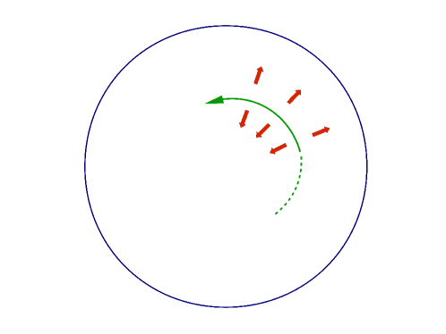
Figure 1: Illustration of the Hall viscosity: a counter-clockwise stirring of the fluid in the bulk of the droplet causes an orthogonal force (red arrows).

Let us analyze the expression of the stress tensor (2.19). Being of first order in time derivatives, it describes a non-covariant effect, in agreement with the fact that the Wen-Zee action is only covariant under time-independent coordinate reparameterization and local frame rotations. At a given time $t=0$ we can choose the conformal gauge for the metric, $g_{ij}(0,x)=\sqrt{g}\,\delta_{ij}$, and consider time-dependent coordinate changes, $\delta x^{i}=u^{i}(t,x)$, representing the deformations. These can be decomposed into conformal transformations and isometries (also called area-preserving diffeomorphisms): the former maintain the metric diagonal and obey $\partial_{i}u_{j}+\partial_{j}u_{i}=\delta_{ij}\,\partial_{k}u^{k}$; the latter keep its determinant constant and satisfy $\partial_{k}u^{k}=0$.

The conformal transformations do not contribute to the stress tensor (2.19); the isometries generated by the scalar function $w(t,x)$ yield:

$$T_{ij}=\eta_{H}\left(2\partial_{i}\partial_{j}-\delta_{ij}\partial^{2}\right)\dot{w},\qquad\quad\delta x^{i}=u^{i}=\varepsilon^{ij}\,\partial_{j}w(t,x)\ .$$ (2.21)

Therefore, we have found that the orthogonal force is proportional to the shear induced in the fluid by time-dependent area-preserving diffeomorphisms.

The last effect parameterized by $\bar{s}$ that we mention in this section is a correction to the density and Hall current in presence of spatially varying electromagnetic backgrounds (in flat space). This is given by [12]:

$$\rho = \frac{\nu}{2\pi}\left(1-\frac{\bar{s}+\bar{s}_{o}}{2}\frac{\partial^{2}}{B_{0}}+O\left(\frac{\partial^{4}}{B_{0}^{2}}\right)\right){\cal B}(x),$$ (2.22)

$$J^{i} = \frac{\nu}{2\pi}\varepsilon^{ij}\left(1-\frac{\bar{s}+\bar{s}_{o}}{2}\frac{\partial^{2}}{B_{0}}+O\left(\frac{\partial^{4}}{B_{0}^{2}}\right)\right){\cal E}^{j}(x).$$ (2.23)

In these equations, the coefficient $\bar{s}$ has an additive non-universal correction $\bar{s}_{o}$ that depends on the value of the gyromagnetic factor in the microscopic Hamiltonian [12][9][26]. The results (2.22, 2.23) do not follow from the Wen-Zee action because they are of higher order in the derivative expansion, i.e. in the series $(\partial^{2}/B_{0})^{n}$ involving the dimensionful parameter $B_{0}$. They were obtained by an independent argument in Ref. [12], and later deduced from the Wen-Zee action upon assuming local Galilean invariance [13]. Our results in this paper will not rely on the presence of this symmetry, and we refer to the works [12][13][14] for an analysis of its consequences.

The correction (2.22) describes an interesting property for the density profile of Laughlin fluids. Numerical and analytical studies of fractional Hall states have found a prominent peak, or overshoot, at the edge (see Fig. 2) [27]. This is in contrast with the integer Hall case, where the profile is monotonically decreasing at the edge. Let us consider the two exact sum rules obeyed by the density of states in the lowest Landau level, specializing to the Laughlin case ($\nu=1/p$). They read:

$$\int d^{2}x\,\rho=N,\qquad\qquad\int d^{2}x\frac{x^{2}}{\ell^{2}}\,\rho=M+N=\frac{pN(N-1)}{2}+N,$$ (2.24)

where $\ell=\sqrt{2\hbar c/eB_{0}}$ is the magnetic length and $M$ is the total angular momentum. The first sum rule is satisfied by a droplet of constant density with sharp boundary, that has the form of a radial step function, $\rho(x)=B_{0}/2p\pi$ for $x^{2}<Np\ell^{2}$, $\rho(x)=0$ for $x^{2}>Np\ell^{2}$. However, inserting this droplet form in the second sum rule only gives the leading $O(N^{2})$ term. This implies that the sub-leading $O(N)$ contribution depends on the shape of the density at the boundary.

We can repeat the calculation with the improved expression of $\rho(x)$ in (2.22): we assume that ${\cal B}(x)$ has the profile of the sharp droplet and compute the sum rules including the $O(\partial^{2}/B_{0})$ correction. Upon integration by parts, this correction vanishes in the first sum rule, while it correctly yields the sub-leading $O(N)$ contribution in the second sum rule, upon matching the parameters $\bar{s}+\bar{s}_{o}=p/2-1$. Of course, changing the profile ${\cal B}(x)$ from a sharp droplet can alter this result by an additive constant; this is another indication that this quantity is not universal. In conclusion, we have found that the intrinsic angular momentum parameter $\bar{s}$ also accounts for the fluctuation of the density profile near the boundary of the droplet.

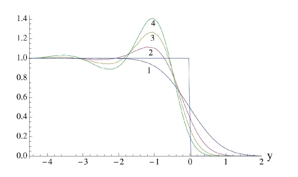
Figure 2: Numerical density profile of the droplet for the $N=200$ electrons Laughlin wavefunction, labeled by the value of $p$ for $\nu=1/p$, from Ref. [27] (the density is normalized to one in the bulk).

3 $W_{\infty}$ symmetry and multipole expansion

3.1 Quantum area-preserving diffeomorphisms

A droplet of two-dimensional incompressible fluid is characterized at the classical level by a constant density $\rho_{0}$ and a sharp boundary. For a circular geometry, the ground state droplet has the shape of a disk and fluctuations amount to shape deformations (see Fig. 3). Given that the number of electrons $N=\rho_{0}A$ is fixed, the area $A$ is a constant of motion, i.e. fluctuations correspond to droplets of same area and different shapes. These configurations of the fluid can be realized by coordinate changes that keep the area constant, i.e. by area-preserving diffeomorphisms [16].

These transformations, already introduced in (2.21), are generated by a scalar function $w(t,x)$; the fluctuations of the density are given by:

$$\delta_{w}\rho=\varepsilon^{ij}\,\partial_{i}\rho\,\partial_{j}w=\left\{\rho,w\right\},\qquad\qquad\delta x^{i}=u^{i}=\varepsilon^{ij}\,\partial_{j}w(t,x)\ ,$$ (3.1)

where we introduced the Poisson bracket over the $(x^{1},x^{2})$ coordinates, in analogy with the canonical transformations of a two-dimensional phase space. The calculation of fluctuations/transformations for the ground state density using (3.1) yields derivatives of the step function that are localized at the edge, as expected [16].

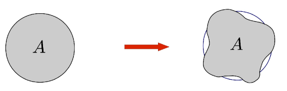
Figure 3: Shape deformation of the droplet under the action of area preserving diffeomorphisms.

It is convenient to introduce the complex notation for the coordinates,

$$z=x^{1}+ix^{2},\quad\bar{z}=x^{1}-ix^{2},\quad ds^{2}=dz\,d\bar{z},\qquad\delta_{z\bar{z}}=\frac{1}{2},\quad\delta^{z\bar{z}}=2,$$ (3.2)

and the corresponding Poisson brackets:

$$\left\{\rho,w\right\}=\varepsilon^{z\bar{z}}\,\partial_{z}\rho\,\partial_{\bar{z}}w+(z\leftrightarrow\bar{z}),\qquad\quad\varepsilon^{z\bar{z}}=-\varepsilon^{\bar{z}z}=-2i\ .$$ (3.3)

A basis of generators can be obtained by expanding the function $w(z,\bar{z})$ in power series,

$${\cal L}_{n,m}=z^{n+1}\,\bar{z}^{m+1},\qquad\qquad w(z,\bar{z})=\sum_{n,m\geq-1}c_{nm}\,z^{n+1}\,\bar{z}^{m+1}\ .$$ (3.4)

The ${\cal L}_{n,m}$ generators obey the so-called $w_{\infty}$ algebra of area-preserving diffeomorphisms,

$$\left\{{\cal L}_{n,m},{\cal L}_{k,l}\right\}=\left((m+1)(k+1)-(n+1)(l+1)\right){\cal L}_{n+k,m+l}\,.$$ (3.5)

We consider now the implementation of this symmetry in the quantum theory of electrons in the lowest Landau level, where coordinates do not commute, i.e. $[\hat{\bar{z}},\hat{z}]=\ell^{2}$. The density and symmetry generators become one-body operators acting in this Hilbert space, that are expressed in terms of bilinears of lowest Landau level field operators $\hat{\Psi}(z,\bar{z})$:

$$\hat{\rho}=\hat{\Psi}^{\dagger}\hat{\Psi},\qquad\hat{\cal L}_{n,m}=\int d^{2}z\,\hat{\Psi}^{\dagger}(z,\bar{z})\,z^{n+1}\,\bar{z}^{m+1}\,\hat{\Psi}(z,\bar{z}),$$ (3.6)

Upon using the (non-local) commutation relations of field operators, one can find the quantum algebra of the generators (3.6) [16],

$$\left[\hat{\mathcal{L}}_{n,m},\hat{\mathcal{L}}_{k,l}\right] = \sum_{s=1}^{\text{Min}(m,k)}\frac{\ell^{2s}\,(m+1)!(k+1)!}{(m-s+1)!(k-s+1)!s!}\ \hat{\mathcal{L}}_{n+k-s+1,m+l-s+1}$$ (3.7)

$$\qquad\qquad-\left(m\leftrightarrow l,\ n\leftrightarrow k\right).$$

This is called the $W_{\infty}$ algebra of quantum area-preserving transformations. The terms on the right hand side form an expansion in powers of $\ell^{2}=2\hbar/B_{0}$: the first term corresponds to the quantization of the classical $w_{\infty}$ algebra (3.5), while the others are higher quantum corrections $O(\hbar^{n})$, $n>1$.

At the quantum level, the classical density given by the ground state expectation value $\rho(z,\bar{z})=\bra{\Omega}\hat{\rho}\ket{\Omega}$, becomes a Wigner phase-space density function, owing to the non-commutativity of coordinates. The quantum fluctuations of the density are given by the commutator with the generator $\hat{w}$ [19],

$$\delta\rho(z,\bar{z})=i\bra{\Omega}[\hat{\rho},\hat{w}]\ket{\Omega}=i\sum_{n=1}^{\infty}\frac{(2\hbar)^{n}}{B_{0}^{n}\ n!}\left(\partial_{\bar{z}}^{n}\rho\ \partial_{z}^{n}w-\partial_{\bar{z}}^{n}w\ \partial_{z}^{n}\rho\right)\equiv\left\{\rho,w\right\}_{M},$$ (3.8)

where $w(z,\bar{z})=\bra{\Omega}\hat{w}\ket{\Omega}$. The non-local expression on the right-hand side is called the Moyal brackets $\{\rho,w\}_{M}$. The leading $O(\hbar)$ term is again the quantum analog of the classical transformation (3.1,3.3). These results are well-known in the lowest Landau level physics; in particular, the algebra of two densities in Fourier space $\hat{\rho}(k,\bar{k})$ is obtained by taking the Moyal brackets (3.8) of two plane waves, leading to the Girvin-MacDonald-Platzman sin-algebra [20].

$$\bra{\Omega}\left[\hat{\rho}(k,\bar{k}),\hat{\rho}(p,\bar{p})\right]\ket{\Omega}=$$

$$\qquad\qquad=\left\{\rho(k,\bar{k}),\rho(p,\bar{p})\right\}_{M}=2\sinh\left(\frac{p\bar{k}-\bar{p}k}{8}\right)\rho(k+p,\bar{k}+\bar{p})\ .$$ (3.9)

The $W_{\infty}$ symmetry of Laughlin and hierarchical fluids has been investigated in several works [16][18], that mainly studied its implementation in the conformal field theory of edge excitations. In the limit to the edge, the density and $W_{\infty}$ generators (3.6) become operators in the $(1+1)$-dimensional theory of the Weyl fermion $\hat{F}$. Their expressions are [17]:

$$\hat{\rho}(R\theta)=\hat{F}^{\dagger}(\theta)\hat{F}(\theta),\qquad\hat{\cal L}_{n,m}=\oint d\theta\,\hat{F}^{\dagger}(\theta)\,e^{i(n-m)\theta}\,\left(i\frac{\partial}{\partial\theta}\right)^{m+1}\,\hat{F}(\theta),$$ (3.10)

where $R\theta$ is the coordinate on the boundary, with $R$ fixed, such that $z\to R\exp(i\theta)$ and $z\bar{z}\sim z\partial_{z}\to i\partial_{\theta}$. Thus, the conformal theory possesses chiral conserved currents of increasing spin (scale dimension), $\sigma=0,1,2,\dots$, whose Fourier components are given by (3.10). These are: the charge $W^{0}=F^{\dagger}F$, the stress tensor $W^{1}\equiv T=F^{\dagger}\partial F$, the spin two field $W^{2}=F^{\dagger}\partial^{2}F$, and so on [17]. The general conformal theories with $W_{\infty}$ symmetry include multicomponent fermionic and bosonic theories and certain coset reductions of them. In particular, the Jain hierarchy of fractional Hall states was uniquely derived by assuming this symmetry and the minimality of the spectrum of excitations [18].

3.2 Higher spin fields

The formula (3.8) of the Moyal brackets is the central point of the following discussion. It expresses the fact that the fluctuations of the density are non-local functions of the density itself. This is not surprising, since any excitation in the lowest Landau level cannot be localized in an area smaller than $\pi\ell^{2}$. Nevertheless, the non-locality is controlled by the $\hbar$, or $1/B_{0}$, expansion. Let us consider (3.8) to the second order in $1/B_{0}$ ($\hbar=1$):

$$\delta\rho \sim \frac{i2}{B_{0}}\,\partial_{\bar{z}}\rho\ \partial_{z}w\,+\frac{2i}{B_{0}^{2}}\,\partial^{2}_{\bar{z}}\rho\,\partial^{2}_{z}w\,+\text{h.c.}$$ (3.11)

$$= -\varepsilon^{z\bar{z}}\left(\frac{1}{B_{0}}\partial_{\bar{z}}\left(\rho\partial_{z}\tilde{w}\right)\ +\ \frac{1}{B_{0}^{2}}\partial^{2}_{\bar{z}}\left(\rho\partial^{2}_{z}w\right)\right)+(z\leftrightarrow\bar{z})\ .$$

In the second line of this equation, we reordered the derivatives and added one scalar term in $w\to\tilde{w}$. The tensor structure of this expression involves a spin one field $(a_{z},a_{\bar{z}})$ and a traceless symmetric tensor field $(b_{zz},b_{\bar{z}\bar{z}})$ in two dimensions as follows:

$$\delta\rho=\varepsilon^{z\bar{z}}\,\partial_{\bar{z}}\left(a_{z}+\frac{1}{2B_{0}}\partial_{\bar{v}}b_{zv}\delta^{\bar{v}v}+\frac{1}{2B_{0}}\partial_{v}b_{z\bar{v}}\delta^{v\bar{v}}\right)+(z\leftrightarrow\bar{z})\ ,$$ (3.12)

since $b_{v\bar{z}}=b_{\bar{z}v}=0$, with $v$ another complex variable. The fields $(a_{z},b_{zz})$ are independent because $\rho,w$ are general functions; they are also irreducible with respect to the O(2) symmetry of the plane.

In the first term of (3.12), we recognize the zero component of the matter current expressed in terms of the hydrodynamic gauge field, $j^{\mu}_{(1)}=\varepsilon^{\mu\nu\rho}\partial_{\nu}a_{\rho}$, as discussed in Section two. Indeed, the other components $j^{i}_{(1)}$, involving also $a_{0}$, are uniquely determined by the requirements of current conservation and gauge invariance of $a_{\mu}$. The second term in (3.12) is similarly rewritten:

$$j^{\mu}_{(2)}=\frac{1}{B_{0}}\varepsilon^{\mu\nu\rho}\partial_{\nu}\,\partial_{k}\,b_{\rho k},\qquad\quad\mu,\nu,\rho=0,1,2,\ \ \ k=1,2,$$ (3.13)

where the components of the spin-two field are $b_{\mu k}=(b_{01},b_{02},b_{11},b_{12},b_{21},b_{22})$ and the summation over spatial indices $k$ is implicit. In this expression, the gauge symmetry,

$$b_{\mu k}\to b_{\mu k}+\partial_{\mu}v_{k}\ ,$$ (3.14)

involving the space vector $v_{k}$, can be used to fix two space components of $b_{jk}$, making it symmetric and traceless. Moreover, the two components $b_{0k}$ will turn out to be Lagrange multipliers, such that the field $b_{\mu k}$ represents two physical degrees of freedom, namely the original $(b_{zz},b_{\bar{z}\bar{z}})$.

In summary, we can view the expansion (3.11) of the Moyal bracket as the gauge-fixed time component of the current:

$$j^{\mu}=j^{\mu}_{(1)}+j^{\mu}_{(2)}=\epsilon^{\mu\nu\rho}\partial_{\nu}a_{\rho}\ +\frac{1}{B_{0}}\epsilon^{\mu\nu\rho}\partial_{\nu}\partial_{k}b_{\rho k}\ .$$ (3.15)

The analysis can be similarly extended to the $O(1/B_{0}^{3})$ term in (3.8) involving the spin three field $c_{\mu kl}$, that is fully symmetric and traceless with respect to its three space indices, and again possesses two physical components, $(c_{zzz},c_{\bar{z}\bar{z}\bar{z}})$; this term will be analyzed in Section 3.5. Continuing the expansion one encounters further irreducible higher-spin fields that are fully traceless and symmetric.

We conclude that the $W_{\infty}$ symmetry of the incompressible fluid in the lowest Landau level shows the existence of non-local fluctuations, that can be made local by expanding in powers of $1/B_{0}$ and introducing a generalized hydrodynamic approach with higher-spin traceless symmetric fields. This is suggestive of a multipole expansion, where the first term reproduces Wen’s theory, and the sub-leading terms give corrections that explore the dipole and higher moments of excitations.

We finally remark that in the expression of the Moyal brackets (3.8), the coefficients of the quantum terms $O(\hbar^{n})$, $n>1$, may depend on the ground state of the system, but the general derivative expansion is kept. The $W_{\infty}$ symmetry also holds for Hall incompressible fluids that fill a finite number of Landau levels beyond the first one [16].

3.3 The effective theory to second order

The construction of the effective theory for the spin-two field $b_{\mu k}$ follows the usual steps described at the beginning of Section 2. We need to couple the current $j^{\mu}_{(2)}$ in (3.13) to the external field $A_{\mu}$ and introduce a dynamics for the new field.

The action for $b_{\mu k}$ should possess the gauge symmetry (3.14), treat the time components $b_{0k}$ non-dynamical and possess as much Lorentz symmetry as possible. To lowest order in derivatives, the following generalized Chern-Simons action satisfies these requirements:

$$S^{(2)}=-\frac{1}{2\gamma B_{0}}\int d^{3}x\,\epsilon^{\mu\nu\rho}\,b_{\mu k}\,\partial_{\nu}b_{\rho k}.$$ (3.16)

The main difference with the standard action for $a_{\mu}$ is the lack of Lorentz symmetry.

In the search of higher-spin field theories in $(2+1)$ dimensions, we can take advantage of the works [22], that have introduced the following family of relativistic actions:

$$S_{CSHS}=\int d^{3}x\,\epsilon^{\mu\nu\rho}\,b_{\mu}^{\{A_{i}\}}\,\partial_{\nu}b_{\rho}^{\{B_{j}\}}\,\delta_{\{A_{i}\}\{B_{j}\}},$$ (3.17)

where $b_{\mu}^{\{A_{i}\}}=b_{\mu}^{A_{1},\cdots,A_{\sigma-1}}$ is totally symmetric with respect to its $(\sigma-1)$ local-Lorentz indices, $A_{i}=0,1,2$, and $\delta_{\{A_{i}\}\{B_{j}\}}$ is the totally symmetric delta function. The actions (3.17) can be made general covariant and reduce to $S^{(2)}$ in the non-relativistic limit (for $\sigma=2$). In the following, we shall keep the discussion as simple as possible and derive the effective action to quadratic order in the fluctuations. In this approximation, we can consider the index $k$ of $b_{\mu k}$ as the space part of a local-Lorentz index. Note also that we do not extend the field $b_{\mu k}\to b_{\mu\nu}$, totally symmetric in $(\mu\nu)$, because in the action (3.16) this would imply a canonical momentum for $b_{0k}$ that is not wanted.

The hydrodynamic effective action for $b_{k}=b_{\mu k}dx^{\mu}$, including the electromagnetic coupling $j^{\mu}_{(2)}A_{\mu}$ is therefore given by:

$$S^{(2)}[b,A]=\int-\frac{1}{2\gamma B_{0}}b_{k}\,d\,b_{k}+\frac{1}{B_{0}}A\,d\,\partial_{k}b_{k}\ .$$ (3.18)

Upon integrating the $b_{k}$ field, one obtains the following contribution to the induced effective action (2.3),

$$S^{(2)}[A]=-\frac{\gamma}{2B_{0}}\int\Delta A\,d\,A\ ,$$ (3.19)

where $\Delta$ is the Laplacian. Therefore, we have obtained the $O(1/B_{0})$ correction to the density and Hall current for slow-varying fields, discussed at the end of Section two, Eqs.(2.22),(2.23).

3.3.1 Coupling to the spatial metric

We now introduce a metric background in the limit of weak gravity and obtain the effective action to quadratic order in the electromagnetic and metric fluctuations. We let interact the metric with the $b_{\mu k}$ field, independently of the $a_{\mu}$ fluctuations, by defining the stress tensor $t^{ik}$ that couples to the metric $g_{ik}$, as follows:

$$t^{\mu k}=\epsilon^{kn}\epsilon^{\mu\nu\rho}\partial_{\nu}b_{\rho n}\ .$$ (3.20)

In this expression, we added the component $t^{0k}$ such that the stress tensor is conserved by construction, $\partial_{\mu}t^{\mu k}=0$. Regarding the space components, we find that the anti-symmetric part,

$$\varepsilon_{ik}t^{ik}=-\varepsilon^{ij}\left(\partial_{j}\,b_{0i}-\partial_{0}\,b_{ji}\right)\ ,$$ (3.21)

is proportional to the Lagrange multiplier $b_{0i}$ that can be put to zero on all observables by a gauge choice. Namely, the stress tensor (3.20) is symmetric “on-shell”.

Some insight on the definition of the stress tensor (3.20) can be obtained by comparing it with the expression (2.1) of the matter current $j^{\mu}_{(1)}$ in terms of the hydrodynamic field $a_{\mu}$. The fluctuation of the charge is given by the integration of the density over the droplet,

$$\delta Q=\int_{D}d^{2}x\,\delta\rho=\oint_{\partial_{D}}dx^{i}a_{i}\,.$$ (3.22)

This reduces to a boundary integral of the hydrodynamic field, as expected for incompressible fluids. Similarly, the integral of the stress tensor gives the momentum fluctuation,

$$\delta P^{k}=\int_{D}d^{2}x\ t^{0k}=\epsilon^{kl}\oint_{\partial D}dx^{i}\ b_{il}=u^{k},$$ (3.23)

that is expressed by the boundary integral of the spin-two hydrodynamic field. Further higher-spin fields measure other tensor quantities at the boundary, thus confirming the picture of the multipole expansion of the droplet dynamics. This argument also gives some indications on the matching between higher-spin fields in the bulk and on the edge (3.10) (the bulk-edge correspondence will be further discussed in the Conclusions).

3.3.2 The Wen-Zee action rederived

Next, we introduce the metric coupling $\lambda\delta g_{\mu k}\,t^{\mu k}$ in the second order action (3.18), including an independent constant $\lambda$ and the component $g_{0k}$ for ease of calculation, to be put to zero at the end:

$$S^{(2)}[b,A,g]=\int-\frac{1}{2\gamma B_{0}}b_{k}\,d\,b_{k}+\frac{1}{B_{0}}A\,d\,\partial_{k}b_{k}+\lambda\delta g_{\mu k}\,\epsilon^{kn}\epsilon^{\mu\nu\rho}\partial_{\nu}b_{\rho n}\ .$$ (3.24)

After integration of $b_{\mu k}$, the induced effective action takes the form:

$$S^{(2)}[A,g]=S^{(2)}_{\text{EM}}[A]+S^{(2)}_{\text{MIX}}[A,g]+S^{(2)}_{\text{GR}}[g],$$ (3.25)

where the three terms read,

$$S^{(2)}_{\text{EM}}[A] = -\frac{\gamma}{2B_{0}}\int d^{3}x\ \epsilon^{\mu\nu\rho}\Delta A_{\mu}\partial_{\nu}A_{\rho}\ ,$$ (3.26)

$$S^{(2)}_{\text{MIX}}[A,g] = -\lambda\gamma\int d^{3}x\ \epsilon^{ij}\epsilon^{kn}\left(A_{0}\partial_{i}-A_{i}\partial_{0}\right)\partial_{k}\delta g_{jn}\ ,$$ (3.27)

$$S^{(2)}_{\text{G}}[g] = -\frac{B_{0}\gamma\lambda^{2}}{2}\int d^{3}x\epsilon^{ij}\delta g_{ik}\delta\dot{g}_{jk}\ .$$ (3.28)

The first term is the $O(1/B_{0})$ electromagnetic correction already found in (3.19). The second and third terms can be rewritten using formulas (2.16) and (2.17) of Section two, as follows:

$$S^{(2)}_{\text{MIX}}[A,g]+S^{(2)}_{\text{G}}[g]=\lambda\gamma\int d^{3}x\left(A_{0}{\cal R}+\varepsilon^{ij}\dot{A}_{i}\Gamma_{j}-\frac{B_{0}\lambda}{2}\varepsilon^{ij}\delta g_{ik}\delta\dot{g}_{jk}\right)\ .$$ (3.29)

We have thus obtained the same expression of the Wen-Zee action (2.18) approximated to quadratic order in the fluctuations. The parameters are identified as,

$$\gamma=\frac{\nu\bar{s}}{2\pi},\qquad\qquad\lambda=\frac{1}{2}\ .$$ (3.30)

Equations (3.24) and (3.29) are the main result of this paper. We have found that the $W_{\infty}$ symmetry of incompressible fluids led to introduce a spin-two hydrodynamic field whose coupling to the metric reproduces Wen-Zee result obtained by coupling the spin connection to the charge current (cf. Eq. (2.8)).

3.4 Universality and other remarks

Let us add some comments:

• The result (3.29) seems to indicate that the gravitational interaction through spin (2.8) of the Wen-Zee approach is equivalent to the coupling to angular momentum of extended excitations.

• Nonetheless, the $W_{\infty}$ symmetry implies the multipole expansion (3.8), whose higher components should yield further geometric terms in the effective action (see next Section).

• In this approach, momentum and charge fluctuations are described by independent fields, $b_{\mu k}$ and $a_{\mu}$, respectively. In the microscopic electron theory, the fixed mass to charge ratio implies the relation $P^{i}=(m/e)J^{i}$ between the two currents; this fact is at the basis of the local Galilean symmetry (Newton-Cartan approach) that has been investigated in the Refs. [12][13][14]. However, in the lowest Landau level $m$ vanishes and the quasiparticle excitations, being composite fermions or dipoles, could have independent momentum and charge fluctuations. In particular, purely neutral excitations at the edge are present for hierarchical Hall fluids [21][18].

• The quadratic action (3.28) is invariant under spatial time-independent reparameterizations within the quadratic approximation. One can easily extend it to be fully space covariant; however, we do not understand at present how to consistently treat the time-dependent non-covariant effects. In particular, there could be several extensions, corresponding to a lack of universality for the results. This point is left to future investigations.

• The $O(1/B_{0})$ correction to the Chern-Simons action provided by $S^{(2)}_{EM}$ in (3.26) is non-universal as already discussed at the end of Section two. Actually, any addition of terms involving powers of the Laplacian and of the curvature,

  $$S[A,g] = \frac{\nu}{4\pi}\int\left[1+\delta_{1}\frac{\Delta}{B_{0}}+\cdots+\beta_{1}\frac{{\cal R}}{B_{0}}+\cdots\right]AdA$$ (3.31)

  $$+ \frac{\nu\bar{s}}{2\pi}\int\left[1+\delta_{2}\frac{\Delta}{B_{0}}+\cdots+\beta_{2}\frac{{\cal R}}{B_{0}}+\cdots\right]Ad\omega\,,$$

  amounts to local deformations that are non-universal (including also the higher-derivative Maxwell term). They can always added a-posteriori in the effective action approach and their coefficients $\delta_{i},\beta_{i},\cdots$ can be tuned at will. In particular, including the Laplacian correction (3.31) into the expression (3.19) and comparing with the known result (2.22), leads to the parameter matching:

  $$\frac{\nu\bar{s}}{4\pi}-\frac{\nu\delta}{4\pi}=\frac{\nu(\bar{s}+\bar{s}_{0})}{8\pi}\ .$$ (3.32)

• Laplacian and curvature corrections to the density and Hall current of Laughlin fluids have been computed to higher order in Refs.[26]. They have been obtained for a clean system without distortions and thus should be considered as fine-tuned for a realistic setting.

• In deriving the effective theory for the $b_{\mu k}$ field, we have assumed its dynamics to be independent from that of $a_{\mu}$. Actually, a non-diagonal Chern-Simons term $\int b_{k}\,d\,\partial_{k}a\$ could be added to the action (3.24), but this would lead to further Laplacian corrections in (3.31).

3.5 The third-order term

The third term in the Moyal brackets (3.8), $\delta\rho\sim i\partial_{\bar{z}}^{3}\rho\,\partial_{z}^{3}w/B^{2}_{0}+{\rm h.c.}$, after reordering of derivatives let us introduce a spin-three field that is totally symmetric and traceless in the space indices, with components $(c_{zzz},c_{\bar{z}\bar{z}\bar{z}})$:

$$\delta\rho_{(3)}=\frac{1}{B^{2}_{0}}\varepsilon^{\bar{z}z}\partial^{3}_{\bar{z}}\,c_{zzz}+{\rm h.c.}\,.$$ (3.33)

This expression can be considered as the gauge fixed, on-shell expression of the following current,

$$j^{\mu}_{(3)}=\frac{1}{B^{2}_{0}}\epsilon^{\mu\nu\rho}\partial_{\nu}\,\partial_{k}\partial_{l}\,P^{k^{\prime}l^{\prime}}_{kl}\,c_{\rho k^{\prime}l^{\prime}},$$ (3.34)

where

$$P^{n^{\prime}l^{\prime}}_{nl}=\frac{1}{2}\left(\delta^{n^{\prime}}_{n}\delta^{l^{\prime}}_{l}+\delta^{n^{\prime}}_{l}\delta^{l^{\prime}}_{n}-\delta_{nl}\delta^{n^{\prime}l^{\prime}}\right)\ ,$$ (3.35)

is the symmetric and traceless projector respect to the $(nl)$ indices. In equation (3.34), the spin-three field $c_{\mu kl}$, traceless symmetric on the $(kl)$ indices, has now six components $c_{\mu kl}=(c_{0zz},c_{0\bar{z}\bar{z}},c_{zzz},c_{\bar{z}zz},c_{z\bar{z}\bar{z}},c_{\bar{z}\bar{z}\bar{z}})$. Two of them can be fixed by the gauge symmetry, $c_{\mu kl}\to c_{\mu kl}+\partial_{\mu}v_{kl}$, with traceless symmetric $v_{kl}$, while the two components with time index are Lagrange multipliers, leading again to two physical components.

The natural form of the coupling of the spin-three field to the metric, although not uniquely justified, is the same as that of the spin-two field (3.20) with an additional derivative:

$$t^{\mu k}_{(2)}=\frac{1}{B_{0}}\epsilon^{kn}\epsilon^{\mu\nu\rho}\partial_{\nu}\partial_{l}\ P^{n^{\prime}l^{\prime}}_{nl}c_{\rho n^{\prime}l^{\prime}},$$ (3.36)

The kinetic term for the spin-three field with the desired gauge symmetry and other properties has again the generalized Chern-Simons form (3.17). In summary, the third-order effective hydrodynamic action is ($c_{kl}=c_{\mu kl}dx^{\mu})$:

$$S_{(3)}[c,A,g]=\int-\frac{1}{2\alpha B^{2}_{0}}c_{kl}\,d\,c_{kl}+A_{\mu}j^{\mu}_{(3)}+\eta\,g_{\mu k}t_{(2)}^{\mu k}\ .$$ (3.37)

The integration over the spin-three field yields the following induced effective action,

$$S^{(3)}[A,g]=S^{(3)}_{\text{EM}}[A]+S^{(3)}_{\text{MIX}}[A,g]+S^{(3)}_{\text{GR}}[g],$$ (3.38)

where:

$$S^{(3)}_{EM}[A] = \frac{\alpha}{4B^{2}_{0}}\int\Delta^{2}\,AdA\,,$$ (3.39)

$$S^{(3)}_{MIX}[A,g] = -\frac{\alpha\eta}{2B_{0}}\int A_{0}\Delta{\cal R}+\varepsilon^{ij}\dot{A}_{i}\Delta\Gamma_{j}\,,$$ (3.40)

$$S^{(3)}_{GR}[g] = \frac{\alpha\eta^{2}}{4}\int\varepsilon^{ij}\delta g_{ik}\Delta\delta\dot{g}_{jk}\,.$$ (3.41)

We thus obtain local Laplacian corrections to the same terms that occur in the second-order action (3.26)-(3.28). This is not surprising because both couplings in (3.37) are derivatives of the lower-order ones (3.24).

It is natural to compare the result (3.41) with the gravitational Wen-Zee action in (2.9)

$$S_{GRWZ}[g] = \xi\int\omega\,d\,\omega=\xi\int\left(\omega_{0}{\cal R}-\varepsilon^{ij}\omega_{i}\,\dot{\omega}_{j}\right)$$ (3.42)

$$\sim \frac{\xi}{4}\int\varepsilon^{ij}\delta g_{ik}\left(\delta_{kl}\Delta-\partial_{k}\partial_{l}\right)\delta\dot{g}_{jl}\,,$$ (3.43)

where $\xi=\left(\nu\bar{s}^{2}-c/12\right)/4\pi$. In the second line of this equation we also wrote the expansion to quadratic order in the fluctuations, to which the cubic term $\omega_{0}{\cal R}$ does not contribute.

Equation (3.43) shows that the gravitational Wen-Zee term contains Laplacian and curvature corrections to the Hall viscosity (2.19). The comparison with the $W_{\infty}$ result (3.41) shows that the expressions of $S^{(3)}_{GR}$ and $S_{GRWZ}$ are similar but not identical, to quadratic order. The explicit calculation of the induced action for integer filling fractions of Ref.[9] is in agreement with (3.41). Following the discussion of universality in Section 3.4, we are lead to conclude that the Laplacian corrections in the third-order $W_{\infty}$ action (3.39-3.41) and the gravitational Wen-Zee term (3.43) are non-universal. We further remark that the curvature correction $\int\omega_{0}{\cal R}$ in (3.42), not obtained in our approach, is believed to be universal because it is also found in the calculation of the Hall viscosity from the Berry phase of the Laughlin wavefunction in a curved background [25].

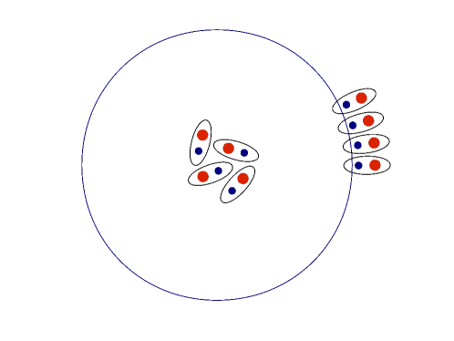
Figure 4: Dipoles aligned at the boundary.

4 The dipole picture

We now present some heuristic arguments that explain two results of the previous sections in terms of simple features of dipoles.

The first observation concerns the fluctuation of the density profile at the boundary (Fig.2). We assume that the low-energy excitations of the fluids are extended objects with a dipole moment; their charge is not vanishing but takes a fractional value due to the unbalance of the two charges in the dipole (numerical evidences of dipoles were first discussed in Ref.[28], to our knowledge). The dipole orientations are randomly distributed in the bulk of the fluid such that they can be approximated by point-like objects with fractional charge (see Fig. 4). However, near the boundary of the droplet, there is a gradient of charge between the interior and the empty exterior; thus, the dipoles align their positive charge tip towards the interior and create the ring-shaped density fluctuation that is observed at the boundary. The effect is stronger for higher dipole moment, that is proportional to $\bar{s}=p/2$, as seen in Fig. 2.

The second effect that can be interpreted in terms of dipoles is the Hall viscosity itself (see Fig. 5). Again the randomly oriented dipoles in the bulk are perturbed by stirring the fluid, namely they acquire an ordered configuration due to the mechanical forces applied. Any kind of ordered configuration of dipoles, such as that depicted in the figure, creates a ring-shaped fluctuation of the density and thus an electrostatic force orthogonal to the fluid motion. This effect is parameterized by the Hall viscosity as discussed in Section two (cf. Fig. 1).

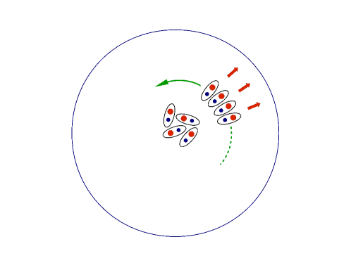
Figure 5: Hall viscosity caused by dipoles aligned along the fluid stream.

The dipole configurations can be matched with the higher-spin field expansion of the density in (3.15), (3.34). We rewrite it as follows:

$$\delta\rho=\varepsilon^{ij}\partial_{i}\left(a_{j}+\frac{1}{B_{0}}\partial_{k}\,b_{jk}+\frac{1}{B_{0}^{2}}\left(\partial_{k}\partial_{l}-\frac{1}{2}\delta_{kl}\Delta\right)c_{jkl}+\cdots\right),$$ (4.1)

and compare to explicit charge configurations. First consider a bulk charge excitation, $\delta\rho(\vec{x})=q\,\delta^{2}(\vec{x})$: this is parameterized by the leading hydrodynamic field $a_{i}\sim O(1/|\vec{x}|)$, as also shown by (3.22). The higher-spin fields do not contribute because they decay faster at $|x|$ infinity, respectively $\partial_{k}b_{jk}\sim O(1/|\vec{x}|^{2})$ and $\partial_{k}\partial_{l}c_{jkl}\sim O(1/\vec{x}|^{3})$, due to the higher derivatives. Next, we analyze a dipole configuration,

$$\delta\rho(\vec{x})=q\left(\delta^{2}(\vec{x}+\vec{d})-\delta^{2}(\vec{x}-\vec{d})\right),$$ (4.2)

that corresponds to a $O(1/|\vec{x}|^{2})$ field, for $|\vec{x}|\gg|\vec{d}|$. In this case, both $a_{j}$ and $b_{jk}$ contribute. It follows that higher moments of the charge configuration gradually involve fields of higher spin values.

We remark that this many-to-one field expansion is a solution for the non-locality of the dynamics. One could consider a redefinition of the expansion (4.1) in terms of a single field, such as $u_{i}=a_{i}+(1/B_{0})\partial_{k}b_{jk}+\cdots$, but this would imply non-local terms in the Chern-Simon actions (3.24), (3.37). Actually, a non-local formulation of Hall physics based on non-commutative Chern-Simons theory has been proposed in Ref. [29], that corresponds to matrix quantum mechanics and matrix quantum fields [30]. We think that the present higher-spin approach shares some features with the non-commutative theory, while being more general and flexible.

5 Conclusions

In this paper, we have used the $W_{\infty}$ symmetry of quantum Hall incompressible fluids to set up a power expansion in the parameter $\hbar/B_{0}$. This analysis leads to a generalized hydrodynamic approach with higher-spin gauge fields, that can be interpreted as a multipole expansion of the extended low-energy excitations of the fluid. To second order, the spin-two field with Chern-Simons dynamics and electromagnetic and metric couplings reproduces the Wen-Zee action. The third-order term yields non-universal corrections to it.

Regarding the universality of terms of the effective action, we have pointed out that local gradient and curvature corrections are non-universal. The universal terms and coefficients can be identified with those that have a correspondence with the conformal field theory on the edge of the droplet. As is well known, the Chern-Simons terms in the effective action,

$$S[a,b,c,\cdots;A,g,\cdots]=-\int\frac{\pi}{\nu}a\,d\,a+\frac{\pi}{\nu\bar{s}B_{0}}b_{k}\,d\,b_{k}+\frac{1}{2\alpha B_{0}^{2}}c_{kl}\,d\,c_{kl}+\cdots+\text{couplings},$$ (5.1)

are not fully gauge invariant and boundary actions are needed to compensate [21].

Typically, the bulk fields define boundary fields that express the boundary action and have spin reduced by one: as is well known, the field $a_{\mu}$ defines through the relation $a_{\mu}=\partial_{\mu}\varphi$ the scalar edge field $\varphi$ that expresses the chiral Luttinger liquid action [21]. Namely, the boundary field is the gauge degrees of freedom that becomes physical at the edge. Similarly, the spin-two field identifies an edge chiral vector, $b_{\mu\theta}=\partial_{\mu}v_{\theta}$, with $\theta$ the azimuthal direction; the spin-three a two-tensor and so on. It follows that the couplings $\nu,\bar{s},\alpha,\cdots$ in (5.1) also appear as parameters in the edge action and can be put in relation with observables of the conformal field theory. Since their values can be related to universal quantities at the edge, these parameters can be defined globally on the system and manifestly do not depend on disorder and other local effects. A hint of this correspondence is already apparent in the quantities (3.22), (3.23) discussed in Section 3.3.1. Let us also mention the work [15] studying the boundary terms of the Wen-Zee action.

The analysis presented in this paper could be developed in many aspects:

• The bulk-edge correspondence for higher-spin actions (5.1) should be developed in detail, and the observables of the conformal field theory should be identified that express the universal parameters. Clearly, the higher-spin fields do not have an independent dynamics at the edge: for Laughlin states, the higher-spin currents are expressed as polynomials of the charge current $\partial_{\theta}\varphi$ [31].

• The third order effective action could encode universal effects if the spin-three hydrodynamic field is coupled to a novel spin-three background ‘metric’, the two fields being related by a Legendre transform. At present we lack a geometric understanding of this and higher-spin background fields, and the physical effects that they describe.

• The analysis presented in this work should be put in contact with the Haldane approach of parametric variations of the Laughlin wavefunction, that also involves a traceless spin-two field [5]. Further deformations could be encoded in the higher-spin background fields mentioned before. Moreover, our approach should be related to the Wiegmann generalized hydrodynamics of electron-vortex composites [6].

• The higher-spin Chern-Simons theories (5.1) predict new statistical phases for dipole monodromies that require physical understanding and verification in model wavefunctions.

• The whole analysis can be extended to the hierarchical Hall states that are described by multicomponent hydrodynamic Chern-Simon fields [21].

Acknowledgments

The authors would like to thank A. G. Abanov, A. Gromov, F. D. M. Haldane, T. H. Hansson, K. Jensen, D. Karabali, S. Klevtsov, V. P. Nair, D. Seminara, D. T. Son, P. Wiegmann and G. R. Zemba for very useful scientific exchanges. A. C. acknowledge the hospitality and support by the Simons Center for Geometry and Physics, Stony Brook, and the G. Galilei Institute for Theoretical Physics, Arcetri, where part of this work was done. The support of the European IRSES grant, ‘Quantum Integrability, Conformal Field Theory and Topological Quantum Computation’ (QICFT) is also acknowledged.

Appendix A Curved space formulas

We consider a spatial metric $g_{ij}=g_{ij}(x^{k},t)$, with $i,j,k=1,2$, depending on space and time and assume that $g_{00}=g_{ij}=0$. This metric can be written in terms of the spatial zweibeins $e^{a}_{i}$ as follows,

$$g_{ij}=e^{a}_{i}e^{b}_{j}\,\delta_{ab},$$ (A.1)

with the coordinates and local frame indices taking the values $i,j,a,b=1,2$. The zweibeins $e^{a}_{i}$ and their inverses $E^{i}_{a}$ satisfy the conditions:

$$E^{i}_{a}e^{a}_{j}=\delta^{i}_{j},\quad\qquad E^{i}_{a}e^{b}_{i}=\delta^{a}_{b}.$$ (A.2)

We also assume that the matrix of vielbeins $e^{A}_{\mu}$ in three dimensions ($\mu,A=0,1,2$), has vanishing space-time and time-time components.

When the gravity background has vanishing torsion, the spin connection can be expressed in terms of the vielbeins [32]. Starting from the three-dimensional expression ($\mu,\nu,\sigma=0,1,2$ and $A,B,C=0,1,2$),

$$\omega_{\mu}^{AB}(e)=\frac{1}{2}\left(E^{\nu[A}\partial_{[\mu}e^{B]}_{\nu]}-E^{\nu[A}E^{B]\sigma}e_{C\mu}\partial_{\nu}e^{C}_{\ \sigma}\right).$$ (A.3)

and the definition,

$$\omega^{C}_{\mu}=\frac{1}{2}\epsilon^{ABC}\omega_{\mu AB},$$ (A.4)

we obtain the following results:

$$\omega^{a}_{\mu}=0,\ \ \ \ a=1,2,$$ (A.5)

$$\omega_{0}\equiv\omega^{0}_{0}=\frac{1}{2}\epsilon^{ab}E^{aj}\partial_{0}e^{b}_{j},$$ (A.6)

and

$$\omega_{i}\equiv\omega^{0}_{i}=\frac{1}{2}\epsilon^{ab}E^{aj}\partial_{i}e^{b}_{j}-\frac{1}{2}\frac{\epsilon^{jk}}{\sqrt{g}}\partial_{j}g_{ki},$$ (A.7)

where $g=\text{det}(g_{ij})$. In the last equation, $\epsilon^{jk}$ is the antisymmetric symbol of coordinate space, $\epsilon^{12}=1$, that is related to that in local frame space as follows:

$$\epsilon^{ab}=\frac{e^{a}_{i}e^{b}_{j}\epsilon^{ij}}{\sqrt{g}},\ \ \ \ \ \ \ \ \epsilon^{ab}E^{ai}E^{bj}=\frac{1}{\sqrt{g}}\epsilon^{ij}.$$ (A.8)

In two spatial dimensions the Riemann tensor $R^{ab}_{ij}$ and the Ricci scalar $\mathcal{R}$ depend on the spin connection through the formulas,

$$R^{ab}_{ij}=\left(\partial_{i}\omega_{j}-\partial_{j}\omega_{i}\right)\epsilon^{ab},\ \ \ \ \ \ \mathcal{R}=2\frac{\partial_{i}\omega_{j}\epsilon^{ij}}{\sqrt{g}}\ .$$ (A.9)

Their coordinate components are written in terms of the Christoffel symbols $\Gamma^{i}_{jk}$ as follows:

$$R^{i}_{jkl}=\partial_{j}\Gamma^{i}_{kl}+\Gamma^{i}_{jr}\Gamma^{r}_{kl}-(j\leftrightarrow k),\ \ \ \ \ \ \ \ \mathcal{R}=g^{jl}R^{k}_{jkl},$$ (A.10)

where

$$\Gamma^{i}_{jk}=\frac{1}{2}g^{il}\left(\partial_{j}g_{lk}+\partial_{k}g_{lj}-\partial_{l}g_{jk}\right).$$ (A.11)

Finally, in curved space the expression for the magnetic field becomes:

$${\cal B}=\frac{\epsilon^{ij}\partial_{i}A_{j}}{\sqrt{g}}.$$ (A.12)

We now find the approximate formulas for small fluctuations around the flat metric, i.e. $g_{ij}=\delta_{ij}+\delta g_{ij}$. Then, $\sqrt{g}\simeq 1$ and $\delta g^{ij}=-\delta g_{ij}$. Choosing a gauge for the local O(2) symmetry such that the zweibeins form a symmetric matrix, we find from (A.1) that:

$$\delta g_{ij}=\delta e^{a}_{j}\delta_{ai}+\delta e^{a}_{i}\delta_{aj}=2\delta e_{ij}.$$ (A.13)

In this limit, an approximate expression for $\omega_{0}$ in (A.6) is obtained by making use of (A.2) and (A.13):

$$\omega_{0}=-\frac{1}{8}\epsilon^{ik}\delta g_{ij}\delta\dot{g}_{kj}.$$ (A.14)

To the linear order, we also find that $\omega_{j}$ in (A.7), $\Gamma^{i}_{jk}$ in (A.11) and the Ricci scalar $\mathcal{R}$ in (A.9) and (A.10) take the following expressions:

$$\omega_{j}=\frac{1}{2}\epsilon^{ki}\partial_{i}\delta g_{kj},$$ (A.15)

$$\Gamma^{i}_{jk}\sim\Gamma_{i,jk}=\frac{1}{2}\left(\partial_{j}\delta g_{ik}+\partial_{k}\delta g_{ij}-\partial_{i}\delta g_{jk}\right),$$ (A.16)

$$\mathcal{R}=\left(\partial_{i}\partial_{j}-\delta_{ij}\partial^{2}\right)\delta g_{ij}.$$ (A.17)

References

- [1] R. E. Prange and S. M. Girvin, The Quantum Hall Effect, Springer, Berlin (1987).
- [2] N. Read and D. Green, “Paired states of fermions in two-dimensions with breaking of parity and time reversal symmetries, and the fractional quantum Hall effect,” Phys. Rev. B 61 (2000) 10267; A. Cappelli, M. Huerta and G. R. Zemba, “Thermal transport in chiral conformal theories and hierarchical quantum Hall states,” Nucl. Phys. B 636 (2002) 568; M. Stone, “Gravitational Anomalies and Thermal Hall effect in Topological Insulators,” Phys. Rev. B 85 (2012) 184503.
- [3] J. E. Avron, R. Seiler and P. G. Zograf, “Viscosity of quantum Hall fluids,” Phys. Rev. Lett. 75 (1995) 697.
- [4] N. Read, “Non-Abelian adiabatic statistics and Hall viscosity in quantum Hall states and p(x) + ip(y) paired superfluids,” Phys. Rev. B 79 (2009) 045308; N. Read and E. H. Rezayi, “Hall viscosity, orbital spin, and geometry: paired superfluids and quantum Hall systems,” Phys. Rev. B 84 (2011) 085316; B. Bradlyn, M. Goldstein and N. Read, “Kubo formulas for viscosity: Hall viscosity, Ward identities, and the relation with conductivity,” Phys. Rev. B 86 (2012) 245309.
- [5] F. D. M. Haldane, “ ”Hall viscosity” and intrinsic metric of incompressible fractional Hall fluids”, arXiv:0906.1854; “Geometrical Description of the Fractional Quantum Hall Effect”, Phys. Rev. Lett. 107 (2011) 116801; “Self-duality and long-wavelength behavior of the Landau-level guiding-center structure function, and the shear modulus of fractional quantum Hall fluids”, arXiv:1112.0990; Y. Park and F. D. M. Haldane, “Guiding-center Hall viscosity and intrinsic dipole moment along edges of incompressible fractional quantum Hall fluids”, Phys. Rev. B 90 (2014) 045123.
- [6] P. B. Wiegmann, “Hydrodynamics of Euler incompressible fluid and the fractional quantum Hall effect”, Phys. Rev. B 88 (2013) 241305(R); P. B. Wiegmann and A. G. Abanov, “Anomalous Hydrodynamics of Two-Dimensional Vortex Fluids,” Phys. Rev. Lett. 113 (2014) 3, 034501.
- [7] J. Fröhlich and U. M. Studer, “Gauge invariance and current algebra in nonrelativistic many body theory,” Rev. Mod. Phys. 65 (1993) 733.
- [8] X. G. Wen and A. Zee, “Shift and spin vector: New topological quantum numbers for the Hall fluids,” Phys. Rev. Lett. 69 (1992) 953 [Phys. Rev. Lett. 69 (1992) 3000].
- [9] A. G. Abanov and A. Gromov, “Electromagnetic and gravitational responses of two-dimensional noninteracting electrons in a background magnetic field,” Phys. Rev. B 90 (2014) 014435.
- [10] G. Y. Cho, Y. You and E. Fradkin, “Geometry of fractional quantum Hall fluids”, Phys. Rev. B 90 (2014) 115139.
- [11] A. Gromov, G. Y. Cho, Y. You, A. G. Abanov and E. Fradkin, “Framing Anomaly in the Effective Theory of the Fractional Quantum Hall Effect”, Phys. Rev. Lett. 114 (2015) 016805.
- [12] C. Hoyos and D. T. Son, “Hall Viscosity and Electromagnetic Response,” Phys. Rev. Lett. 108 (2012) 066805.
- [13] D. T. Son, “Newton-Cartan Geometry and the Quantum Hall Effect”, arXiv:1306.0638; M. Geracie, D. T. Son, C. Wu and S. F. Wu, “Spacetime symmetries of the quantum Hall effect”, Phys. Rev. D 91 (2015) 045030; B. Bradlyn and N. Read, “Low-energy effective theory in the bulk for transport in a topological phase,” Phys. Rev. B 91 (2015) 125303.
- [14] A. G. Abanov and A. Gromov, “Density-Curvature Response and Gravitational Anomaly” Phys. Rev. Lett. 113 (2014) 266802; “Thermal Hall Effect and Geometry with Torsion” Phys. Rev. Lett. 114 (2014) 016802;
- [15] S. Moroz, C. Hoyos and L. Radzihovsky, “Galilean invariance at quantum Hall edge,” Phys. Rev. B 91 (2015) 195409; A. Gromov, K. Jensen and A. G. Abanov, “Boundary effective action for quantum Hall states”, arXiv:1506.07171.
- [16] A. Cappelli, C. A. Trugenberger and G. R. Zemba, “Infinite symmetry in the quantum Hall effect,” Nucl. Phys. B 396 (1993) 465; “Large N limit in the quantum Hall Effect,” Phys. Lett. B 306 (1993) 100.
- [17] A. Cappelli, G. V. Dunne, C. A. Trugenberger and G. R. Zemba, “Conformal symmetry and universal properties of quantum Hall states,” Nucl. Phys. B 398 (1993) 531; A. Cappelli, C. A. Trugenberger and G. R. Zemba, “W(1+infinity) dynamics of edge excitations in the quantum Hall effect,” Annals Phys. 246 (1996) 86; “Classification of quantum Hall universality classes by W(1+infinity) symmetry,”, Phys. Rev. Lett. 72 (1994) 1902.
- [18] A. Cappelli, C. A. Trugenberger and G. R. Zemba, “Stable hierarchical quantum hall fluids as W(1+infinity) minimal models,” Nucl. Phys. B 448 (1995) 470; “W(1+infinity) minimal models and the hierarchy of the quantum Hall effect,” Nucl. Phys. Proc. Suppl. 45A (1996) 112 [Lect. Notes Phys. 469 (1996) 249]; A. Cappelli and G. R. Zemba, “Hamiltonian formulation of the W (1+infinity) minimal models,” Nucl. Phys. B 540 (1999) 610.
- [19] S. Iso, D. Karabali and B. Sakita, “Fermions in the lowest Landau level: Bosonization, W infinity algebra, droplets, chiral bosons,” Phys. Lett. B 296 (1992) 143; “One-dimensional fermions as two-dimensional droplets via Chern-Simons theory,” Nucl. Phys. B 388 (1992) 700; B. Sakita, “W(infinity) gauge transformations and the electromagnetic interactions of electrons in the lowest Landau level,” Phys. Lett. B 315 (1993) 124.
- [20] S. M. Girvin, A. H. MacDonald and P. M. Platzman, “Magneto-roton theory of collective excitations in the fractional quantum Hall effect,” Phys. Rev. B 33 (1986) 2481.
- [21] X. G. Wen, Quantum Field Theory of Many-body Systems, Oxford Univ. Press, Oxford (2007).
- [22] A. Campoleoni, S. Fredenhagen, S. Pfenninger and S. Theisen, “Asymptotic symmetries of three-dimensional gravity coupled to higher-spin fields”, JHEP11 (2010) 007; A. Campoleoni, S. Fredenhagen and S. Pfenninger, “Asymptotic W-symmetries in three-dimensional higher-spin gauge theories”, JHEP09 (2011) 113; M. R. Gaberdiel and R. Gopakumar, “An dual for minimal model CFTs”, Phys. Rev. D 83 (2011) 066007.
- [23] L. D. Landau and E. M. Lifshitz, Theory of Elasticity, 3rd ed., Pergamon Press, Oxford (1986).
- [24] T. L. Hughes, R. G. Leigh and O. Parrikar, “Torsional Anomalies, Hall Viscosity, and Bulk-boundary Correspondence in Topological States,” Phys. Rev. D 88 (2013) 025040.
- [25] B. Bradlyn and N. Read, “Topological central charge from Berry curvature: Gravitational anomalies in trial wave functions for topological phases,” Phys. Rev. B 91 (2015) 165306; S. Klevtsov and P. Wiegmann, “Geometric adiabatic transport in quantum Hall states,” Phys. Rev. Lett. 115 (2015) 086801.
- [26] S. Klevtsov, “Random normal matrices, Bergman kernel and projective embeddings,” JHEP 1401 (2014) 133; F. Ferrari and S. Klevtsov, “FQHE on curved backgrounds, free fields and large N,” JHEP 1412 (2014) 086; T. Can, M. Laskin and P. Wiegmann, “Geometry of Quantum Hall States: Gravitational Anomaly and Kinetic Coefficients”, Annals Phys. 362 (2015) 752.
- [27] N. Datta, R. Morf and R. Ferrari, “Edge of the Laughlin droplet, ” Phys. Rev. B 53, 10906 (1996); T. Can, P. J. Forrester, G. Téllez and P. Wiegmann “Singular behavior at the edge of Laughlin states” Phys. Rev. B 89 (2014) 235137.
- [28] J. K. Jain, R. K. Kamilla, “Composite Fermions in the Hilbert Space of the Lowest Electronic Landau Level” Int. J. Mod. Phys. B 11, 2621 (1997).
- [29] L. Susskind, “The Quantum Hall fluid and noncommutative Chern-Simons theory,” arXiv:hep-th/0101029.
- [30] A. P. Polychronakos, “Quantum Hall states as matrix Chern-Simons theory,” JHEP 0104 (2001) 011; A. Cappelli and I. D. Rodriguez, “Matrix Effective Theories of the Fractional Quantum Hall effect,” J. Phys. A 42 (2009) 304006.
- [31] A. Cappelli, C. A. Trugenberger and G. R. Zemba, “W(1+infinity) dynamics of edge excitations in the quantum Hall effect,” Annals Phys. 246 (1996) 86.
- [32] D. Z. Freedman and A. Van Proeyen, Supergravity, Cambridge Univ. Press, Cambridge (2012).