On orienting edges of unstructured two- and three-dimensional meshes

Abstract

Finite element codes typically use data structures that represent unstructured meshes as collections of cells, faces, and edges, each of which require associated coordinate systems. One then needs to store how the coordinate system of each edge relates to that of neighboring cells. On the other hand, we can simplify data structures and algorithms if we can a priori orient coordinate systems in such a way that the coordinate systems on the edges follow uniquely from those on the cells by rule.

Such rules require that every unstructured mesh allows the assignment of directions to edges that satisfy the convention in adjacent cells. We show that the convention chosen for unstructured quadrilateral meshes in the deal.II library always allows to orient meshes. It can therefore be used to make codes simpler, faster, and less bug prone. We present an algorithm that orients meshes in $O(N)$ operations. We then show that consistent orientations are not always possible for 3d hexahedral meshes. Thus, cells generally need to store the direction of adjacent edges, but our approach also allows the characterization of cases where this is not necessary. The 3d extension of our algorithm either orients edges consistently, or aborts, both within $O(N)$ steps.

1 Introduction

In most of the common numerical methods for the solution of partial differential equations on bounded domains $\Omega\subset{\mathbb{R}}^{d},d=2,3$, one defines approximate solutions by first subdividing $\Omega$ into a finite number of cells, and then setting up a system of equations on these cells. Usually, cells are either triangular or quadrilateral (for $d=2$), or tetrahedral, prismatic, pyramidal, or hexahedral (for $d=3$). Because certain aspects of the solution may be associated with cells or edges (in 2d), or cells, faces and edges (in 3d), essentially all sufficiently general codes use data structures for such meshes that explicitly or implicitly store not only cells and vertex locations, but also faces and edges and allow associating data with these objects.

In many cases, the data that is associated with a cell, face, edge, or vertex may have a physical location somewhere on this object. For example, when using a ${\mathbb{Q}}_{3}$ bicubic finite element on a rectangular cell, we need to store the index (and possibly the value) of one degree of freedom per vertex, two along the edge (typically at 1/3 and 2/3 along its extent), and 4 inside the cell. In order to define where a distance of 1/3 or 2/3 along the edge is, we need to define a coordinate system on the edge. The same is true when implementing Nédélec elements that define degrees of freedom as tangential vectors along edges, and therefore need to define a direction on each edge. For similar reasons, we typically also need coordinate systems within each cell.

We then need to define how the coordinate system defined on the edge relates to that of the adjacent cells. We can either do this by letting every quadrilateral cell store pointers to the four edges along with one bit per edge that indicates how the direction of the edge embeds in the coordinate system of the cell. Or we could seek a convention by which we orient all edges of the mesh once at the beginning so that the orientation of each cell implies the orientation of its bounding edges. In the latter case, we would not need to store direction flags, and algorithms built on this convention would not need to provision for different possible directions, thereby greatly simplifying code construction and maintenance.

This paper is concerned with the following two questions:

• Is it possible to find such a convention for quadrilateral meshes (an example of such a mesh is shown in Fig. 1)? We will constructively show that this is indeed possible in 2d when adopting the convention that the edges that bound opposite sides of each cell point in the same direction; see the left panel of Fig. 2.

• Is it possible to assign directions to all edges of a mesh that satisfy this convention in a computationally efficient manner? We will demonstrate that this is in fact so: Our construction of a proof for the answer to the first question (in Section 3) also implies an algorithm that we show to be order optimal, i.e., it runs in a time proportional to the number of edges in the mesh.

. .

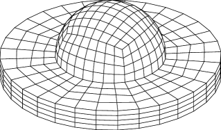
Figure 1: A typical two-dimensional quadrilateral mesh around an airfoil with 29,490 cells (left). Surface of a three-dimensional mesh with 2,304 cells (right).

. .

Figure 2: Choice of directions of edges when seen with regard to one particular orientation of a “coordinate system” on a cell. Note in particular that this choice implies that opposite edges in a cell must have parallel directions. Left: For quadrilaterals in $d=2$. Right: For hexahedra in $d=3$.

On the other hand, we will show in Section 4 that the corresponding convention in 3d (see the right panel of Fig. 2) allows for examples where it is not possible to orient edges so that coordinate systems of adjacent cells are implied. However, we will show that the extension of the 2d algorithm to 3d either produces a consistent set of edge orientations or fails, both within order optimal complexity. There are, however, important classes of 3d meshes that always allow such edge directions, and we will discuss these in Section 5.

The paper is complemented by Section 2 defining notation, conclusions in Section 6, and an appendix in which we we prove a generalization of the main statement of the paper to general manifolds.

Related literature

Finite element software packages have traditionally taken different routes to dealing with the problem of relative orientations of cells and their edges and faces. In many cases, software has been developed to only support linear or quadratic $H^{1}$-type elements, in which case edge and face orientations are not in fact of any concern at all. Others use triangular or tetrahedral meshes for which it is necessary to explicitly store edge orientations; see, for example, [5, 1]. For quadrilaterals and hexahedra, strategies for implementation in specific packages are discussed in [17] for the FEniCS library and [20] for the KARDOS package. We have found that DUNE [4] and Nektar++ [7] appear to explicitly store edge directions as part of their mesh data structures or finite element implementations, but we could not find written elaborations of their strategies in publications or overview documents. Finally, descriptions of finite elements that use global conventions for edge orientations (i.e., based on vertex coordinates or indices, instead of in relation to locally adjacent cells) can be found in [21] and are used, for example, in libMesh [12].

Constructions similar to those in this paper have previously been discussed in the discrete geometry literature, see [10, 18, 9] for examples. However, this part of the literature is not typically concerned with algorithms and their complexity (such as our discussions in Sections 3 and 4), nor with the particular application of these ideas to finite element meshes (such as our discussion of specific types of meshes in Section 5). Our contribution therefore provides a relevant extension of what is available in the literature.

A historical note

The algorithms discussed herein were implemented in the deal.II library in 2003, with an incomplete discussion of the topic available in the documentation of deal.II’s GridReordering class. A more formal description of these algorithms has recently appeared in [11]; it extends our 2d algorithms to meshes stored on distributed memory, parallel machines, but it lacks the complexity analysis that we provide here, as well as much of the discussion of the 3d case.

The introduction in deal.II of the convention discussed above predates 2003. In its earliest days, the library was almost always used on small problems for which edge orientations could be determined by hand on a piece of paper, and little consideration was given to the question whether it always exists and if so whether there is an efficient algorithm to generate it automatically. However, as the project grew and more applications used the 3d part, these questions became more important. Initially, an algorithm that generated edge orientations using a backtracking algorithm was implemented. This works for meshes with up to a few hundred cells, but fails due to excessive run times for larger ones. In particular, it is easy to construct meshes for which it had exponential run time. Therefore, more efficient algorithms were needed, leading to the results reported here.

Availability of implementations

We have implemented the algorithms outlined here in the deal.II library (see http://www.dealii.org/ and [2, 3]), and they are available as part of the GridReordering class under the LGPL open source license.

2 Notation and conventions

Throughout this paper, we will consider triangulations ${\mathbb{T}}$ such as those shown in Fig. 1, as a collection ${\mathbb{T}}=\{K_{1},\ldots,K_{N_{K}}\}$ of quadrilateral or hexahedral cells $K_{i}$. These cells can be considered as open geometric objects $K_{i}\subset{\mathbb{R}}^{d},d=2,3$ so that (i) $K_{i}\cap K_{j}=\emptyset$ if $i\neq j$, (ii) the intersection of the closure of two cells, $\bar{K}_{i}\cap\bar{K}_{j}$, is either empty, a vertex of the mesh, or a complete edge or face of both cells, and (iii) $\bigcup_{i}\bar{K}_{i}=\bar{\Omega}$ where $\Omega\subset{\mathbb{R}}^{d}$ is the bounded, open domain that is subdivided into the triangulation. We assume that the triangulation has only finitely many cells. For the purposes of this paper, we do not require that the union of mesh cells corresponds to a simply connected domain. We will rely on the very practical assumption that the volume of each cell is positive and that cells are convex.

That said, the bulk of our arguments will not make use of this geometric view of a triangulation. Rather, it is convenient to reformulate the problem under consideration using the language of graphs. When viewing a finite element mesh as an undirected graph, we consider it as a pair $G_{\mathbb{T}}=(V,E)$ with the vertices $V=\{v_{1},\ldots,v_{N_{v}}\}$ being the vertices of the mesh, and edges $E=\{e_{1},\ldots,e_{N_{e}}\}\subset\{\{v_{a},v_{b}\}:v_{a},v_{b}\in V,v_{a}\neq v_{b}\}$ being the four ($d=2$) or twelve ($d=3$) edges of the cells. Given the construction of this graph as a representation of a mesh, there is then a collection of cells ${\mathbb{T}}=\{K_{1},\ldots,K_{N_{K}}\}$ where we can alternatively see each $K_{i}$ as either an ordered collection of 4 vertices or an ordered collection of 4 edges (in 2d; in 3d it is 8 vertices and 12 edges). The index ${\mathbb{T}}$ on $G_{\mathbb{T}}$ indicates that we are not considering general graphs but indeed only those graphs that originate from a triangulation of a domain $\Omega\subset{\mathbb{R}}^{d}$.

For a given cell $K$, let $v(K)\subseteq V$ be the set of its vertices and $e(K)\subseteq E$ the set of its edges. For a given edge, let $K(e)\subseteq{{\mathbb{T}}}$ be the set of adjacent cells. In 2d, $|K(e)|$ is either one or two (depending on whether the edge is at the boundary or not); in 3d, $|K(e)|\geq 1$ since arbitrarily many cells may be adjacent to a single edge.

As discussed above, we are interested in assigning a direction to each edge in such a way that the direction of the edge is implied from the orientation of a cell. That is, for a mesh with associated graph $G_{\mathbb{T}}$, we would like to have a directed graph $G_{\mathbb{T}}^{+}=(V,E^{+})$ with the same vertex set and edges, but where each edge is now considered directed (i.e., represented by an ordered pair of vertices). To be precise, this graph is in fact oriented since we never have both $(v_{i},v_{j})\in E^{+}$ and $(v_{j},v_{i})\in E^{+}$ as may occur in directed graphs.

2.1 Goals for orienting meshes

As discussed in the introduction, practical implementations of the finite element method need to define a coordinate system on both cells and edges of a mesh. This is typically done by mapping a reference cell $\hat{K}=[0,1]^{d}$ and edge $\hat{e}=[0,1]$ to each cell $K$ and edge $e$, along with the coordinate systems. The details of this are of no importance here other than the following two statements: (i) On each cell, we need to designate one of the four (or eight) vertices as the “origin”; each of the two (three) edges adjacent to the origin then form the first and second (and third) “coordinate axis”. If we insist that the mapping from the reference cell $\hat{K}$ to $K$ has positive volume, then the choice of the origin fixes the coordinate system in 2d; in 3d, each of the edges adjacent to the origin can be chosen as the first coordinate axis, with the other two then fixed. In other words, each cell allows for 4 possible choices of coordinate systems in 2d, and $8\times 3=24$ in 3d. (ii) On each edge, we define a coordinate system by choosing a “first” vertex.

With this, there are a total of $4^{|N_{K}|}$ choices in 2d for the coordinate systems on the cells (and $24^{|N_{K}|}$ in 3d), and $2^{|N_{e}|}$ for the coordinate systems of the edges. The question is now whether it is possible to choose them in such a way that if the coordinate systems of all cells are specified, we can infer the coordinate system on each edge unambiguously, regardless of which cell adjacent to the edge we consider. Or conversely: is it possible to specify directions for all edges in such a way that this implies a unique choice of coordinate systems for all cells?

For reasons that will become clear later, we will prescribe directions of the edges of a cell when seen in the “coordinate system” of the cell as shown in Fig. 2. Clearly, it will be possible to choose the coordinate systems of two neighboring cells in such a way that they do not agree on the direction of the common edge. Such a choice would require an implementation to store for each cell whether or not an edge’s (global) direction does or does not match the direction that results from the (local) convention.

On the other hand, let us assume that we can find an orientation for all edges of the mesh so that in each cell, “opposite” edges are “parallel”. Then each cell has one vertex from which all oriented edges originate, and we can choose this as the “origin” of the cell. Using this choice of cell coordinate system, edge directions are then again uniquely implied and the problem is solved. In other words, we have reduced the problem of orienting all cells and edges to the problem of finding one particular set of edge orientations that satisfy the “opposite” edges are “parallel” property.

This property is easy to understand intuitively. It is significantly more cumbersome to describe it rigorously in the graph theoretical language, and so we will only do this for the 2d case. (The 3d case follows the same approach but requires lengthy notation despite the fact that the situation is relatively easy to understand.) In order to formulate the convention, we need to fix the order in which we consider vertices and edges as part of a cell. We do so using a lexicographic order for vertices, as shown in Fig. 3. Edges are numbered so that we first number the edge from vertex 0 to 2, then its translation in the perpendicular direction (i.e., from vertex 1 to 3), and then the edges connecting the vertices of the first two edges. Both of these orders reflect the tensor product structure of quadrilaterals and are easily generalized to hexahedra (or higher dimensions, if desired). The choice of edge directions within each cell, as shown in Fig. 2, then ensures that the coordinate system of the edge is simply the restriction of the cell’s coordinate system to the edge.

. .

Figure 3: Numbering convention for vertices and edges of two-dimensional cells. Here, $v(K)^{+}$ is the ordered set of vertices that bound the cell, and $e(K)^{+}$ the ordered set of edges.

With this definition, each cell is described by an ordered tuple of its vertices where we will assume that the first element of this tuple corresponds to the “origin”. Equivalently, we can describe each cell as an ordered tuple of four (unordered) edges, where the “origin” of the cell is now the common vertex of edges 0 and 2. Because there are 4 possible choices for the origin of the cell, there are four ways to describe a cell that are equivalent up to rotation.

With these preparations, we can finally define what it means for the edges of a directed graph $G_{\mathbb{T}}^{+}$ that represents a quadrilateral mesh to be consistently oriented:

Convention 1.

We call a graph $G_{\mathbb{T}}^{+}=(V,E^{+})$ consistently oriented with respect to cell $K\in{\mathbb{T}}$ if among the four equivalent choices of vertex tuples of $K$, there is one so that the following directed edges are all elements of $E^{+}$: $e(K)_{0}=(v(K)_{0},v(K)_{2})$, $e(K)_{1}=(v(K)_{1},v(K)_{3})$, $e(K)_{2}=(v(K)_{0},v(K)_{1})$, $e(K)_{3}=(v(K)_{2},v(K)_{3})$.

Convention 2.

We call a graph $G_{\mathbb{T}}^{+}=(V,E^{+})$ consistently oriented if it is consistently oriented with respect to all cells in ${\mathbb{T}}$.

As discussed above, a consistently oriented graph has edges that allow us to choose a coordinate system on each cell so that the edge orientations follow immediately from the cell orientations. Similar definitions can be given for the 3d case. The purpose of this paper is to ask the question whether it is always possible to consistently orient the edges of a given mesh ${\mathbb{T}}$, and if this is the case, whether it can efficiently be done by an algorithm.

2.2 Reformulation of Conventions 1 and 2

The developments in the following sections all depend on the fact that Convention 1 can equivalently be stated by only looking at sets of “parallel edges” of quadrilaterals:

Definition 3.

Two edges $e^{\prime},e^{\prime\prime}\in E$ are called parallel edges of $K$ if $e^{\prime}=e^{\prime\prime}$ or if they bound $K$ but do not share a vertex. If $e^{\prime},e^{\prime\prime}\in E$ are parallel edges of $K$, then we denote $e^{\prime}\mathrel{\|_{K}}e^{\prime\prime}$. We say that $e^{\prime},e^{\prime\prime}\in E$ are locally parallel and denote $e^{\prime}\mathrel{\|_{*}}e^{\prime\prime}$ if there exists a cell $K\in{\cal K}$ so that $e^{\prime}\mathrel{\|_{K}}e^{\prime\prime}$.

The four edges of a quadrilateral then fall into two classes of two edges each that are parallel. (In 3d, a corresponding but more notationally cumbersome definition would yield three classes of four parallel edges each.) In practice, one does not usually have to verify if edges are parallel, but only enumerate classes of parallel edges; this does not require testing all equivalent edge sets: in 2d, edges $e(K)_{0}$ and $e(K)_{1}$ are parallel, as are $e(K)_{2}$ and $e(K)_{3}$, for any arbitrarily chosen equivalent edge set. We can then define consistent orientations via these classes of parallel edges:

Convention 4.

Two oriented, parallel edges $e^{\prime},e^{\prime\prime}\in E^{+}$ are called consistently oriented with respect to cell $K$ if $e^{\prime}=(v(K)_{0},v(K)_{2})$, $e^{\prime\prime}=(v(K)_{1},v(K)_{3})$ with regard to the one equivalent vertex set within which $e^{\prime}=e(K)_{0}$ and $e^{\prime\prime}=e(K)_{1}$.

Convention 5.

We call a graph $G_{\mathbb{T}}^{+}=(V,E^{+})$ consistently oriented with respect to cell $K$ if all sets of parallel edges of $K$ are consistently oriented with regard to $K$.

In other words, consistent orientation on a cell can be tested by only verifying consistent orientation of all the edges in all sets of parallel edges. Consequently, testing that a graph $G_{\mathbb{T}}^{+}$ is consistently oriented is relatively easy and can be done by verifying the condition on every cell separately. A verification algorithm can therefore easily be written with $O(N_{K})$ complexity and, consequently, with $O(N_{e})$ because $\frac{1}{2}N_{K}\leq N_{e}\leq 4N_{K}$. On the other hand, generating a consistent orientation requires a global algorithm because the orientation of one edge implies that of all of its parallel edges on all of its adjacent cells, which itself implies the orientation of edges parallel on cells twice removed, etc. Because of this property, it is not a priori clear that one can find a linear-time algorithm that can find a consistently oriented graph $G_{\mathbb{T}}^{+}$ given the graph $G_{\mathbb{T}}$ associated with a mesh. However, as we will show below, this is indeed possible.

As a final note in this section, let us state that for all algorithms that follow, we assume that we have methods to generate the vertex and edge sets $v(K),e(K)$ for a given cell $K$ with ${\cal O}(1)$ complexity. This can easily be achieved by storing this information as the rows of $N_{K}\times 4$ matrices as is commonly done in all widely used software (in 3d, the vertex adjacency matrix is of size $N_{K}\times 8$ and the edge adjacency matrix is of size $N_{K}\times 12$). Furthermore, we will assume that finding the cell neighbors of a given edge, $K(e)$, requires ${\cal O}(1)$ time. It is obvious that in 2d, this can be achieved by storing an $N_{e}\times 2$ matrix storing the indices of the one or two cells that are adjacent to each edge; populating this matrix from $e(K)$ requires only a single loop over all cells. In 3d, the number of cells adjacent to each cell can in principle be equal to $N_{K}$, requiring data structures that can either not be queried in ${\cal O}(1)$ complexity, or can not be built with ${\cal O}(N_{K})$ complexity; however, in actual finite element practice, the meshes we consider will never have more than, say, a dozen or so elements joined at any one edge, so that we can consider $|K(e)|$ to be bounded by a constant, thereby allowing storing information in tables of fixed width and ensuring that $K(e)$ can be queried with ${\cal O}(1)$ complexity. These assumptions will be important to guarantee the overall complexity of the algorithms we will consider in the following.

As stated above, we assume that $K(e)$ can be evaluated in ${\cal O}(1)$ time. To make this possible requires building appropriate data structures, and depending on what information is available this may require more than ${\cal O}(N)$ time. For example, if one only knew the vertices of each cell, i.e., $v(K)$, then building tables that can evaluate $e(K)$ in ${\cal O}(1)$ time requires ${\cal O}(N\,\log N)$ time; this is the typical case with file formats that store mesh information. On the other hand, if each cell already knows all of its edge neighbors, as is often the case inside mesh generators or finite element codes, then building the tables to evaluate $e(K)$ in ${\cal O}(1)$ only costs ${\cal O}(N)$ time and is consequently of the same complexity as the algorithms we will discuss in the following.

3 The two-dimensional case

In this section, we will consider the two-dimensional problem, which can be stated as follows: Given a graph $G_{\mathbb{T}}$ that originates from a mesh ${\mathbb{T}}$ composed of quadrilaterals, find a consistently oriented graph $G_{\mathbb{T}}^{+}$.

As mentioned above, consistency of edge directions only requires us to ensure consistency within sets of parallel edges. To this end, we will in the following describe methods that first find all edges that are, in some sense that goes beyond that defined in Definition 3, parallel to each other (Section 3.1). We will then show how we can consistently orient all edges that are in this sense parallel to each other (Section 3.2) and finally how we can orient all edges in the graph (Section 3.3).

3.1 Decomposing $E$ into sets of parallel edges

As we will show next, the set of edges $E$ of $G_{\mathbb{T}}$ can be decomposed into a collection of mutually exclusive sets of edges, where the edges in each set are all parallel to each other in some global sense. This follows from the fact that the relation locally parallel is reflexive (i.e., $e\mathrel{\|_{*}}e$ for all edges $e$) and symmetric (i.e. $e^{\prime}\mathrel{\|_{*}}e^{\prime\prime}$ implies $e^{\prime\prime}\mathrel{\|_{*}}e^{\prime}$ for all edges $e^{\prime},e^{\prime\prime}$) by construction. Let us define two edges $e^{\prime}$, $e^{\prime\prime}$ to be globally parallel if there is a finite, possibly empty sequence of edges $e_{0},e_{1},\ldots,e_{s}$ such that $e^{\prime}\mathrel{\|_{*}}e_{0}\mathrel{\|_{*}}e_{1}\mathrel{\|_{*}}\ldots\mathrel{\|_{*}}e_{s}\mathrel{\|_{*}}e^{\prime\prime}$ and denote this by $e^{\prime}\mathrel{\|}e^{\prime\prime}$. One immediately checks that this relation is reflexive, symmetric and transitive (i.e. $e^{\prime}\mathrel{\|}e^{\prime\prime}$ and $e^{\prime\prime}\mathrel{\|}e^{\prime\prime\prime}$ imply $e^{\prime}\mathrel{\|}e^{\prime\prime\prime}$ for all edges $e^{\prime},e^{\prime\prime},e^{\prime\prime\prime}$) and hence forms an equivalence relation. This relation then partitions $E$ into disjoint sets of (globally) parallel edges [13, Chapter I, §3] or [15, Corollary 28.19].

Algorithmically, we can recursively construct each of these sets by starting with an edge $e$ and build the set $\Pi(e)\subseteq E$ of all edges that are globally parallel to $e$ by first adding the edges opposite $e$ in the cells adjacent to $e$, then those edges that are opposite to the ones added previously, and so on. Sets of parallel edges are central to the rest of the paper, since our edge direction convention requires that they will all have parallel directions. An intuitive interpretation of the importance of parallel edges is as follows: assume we had already found the directed graph $G_{\mathbb{T}}^{+}$. Then, flipping the direction of an edge $e$ would make the triangulation non-consistent, and to make it consistent again we would have to flip the directions of a number of other edges as well; the entire set of edges that needs to be flipped, including $e$, is precisely $\Pi(e)$.

With this knowledge, let us concisely define an algorithm to find all elements of a parallel set for an edge $e$ as a first step:

Algorithm 6 ((Construct one set of parallel edges)).

Let $e\in E$ be a given edge and generate the set $\Pi(e)$ of edges parallel to $e$ recursively as follows, where the set $\Delta_{k}$ consists of those edges that we add to $\Pi(e)$ in each step as we grow it away from $e$:

1. Set $\Pi_{0}(e)=\emptyset$, $\Pi_{1}(e)=\{e\}$, $\Delta_{0}=\{e\}$, $k=1$.

2. While $\Delta_{k-1}\neq\emptyset$, do:

   1. Set $\Delta_{k}=\emptyset$.

   2. For each $\delta\in\Delta_{k-1}$:

      • Set ${\cal E}(\delta)=\emptyset$.

      • For each $K\in K(\delta)$:

        1. Set ${\cal N}_{K}(\delta):=\{\varepsilon\in e(K):\varepsilon\mathrel{\|_{K}}\delta\}\backslash\{\delta\}$.

        2. Set ${\cal E}(\delta)={\cal E}(\delta)\cup{\cal N}_{K}(\delta)$.

      • Set $\Delta_{k}=\Delta_{k}\cup\left({\cal E}(\delta)\backslash\Pi_{k}(e))\right)$.

   3. $\Pi_{k+1}(e)=\Pi_{k}(e)\cup\Delta_{k}$.

   4. Set $k:=k+1$.

3. Set $\Pi(e)=\Pi_{k}(e)$.

Fig. 4 gives a graphical depiction of the construction of one such set. Starting from a given edge $e$, the set $\Pi(e)$ grows in each step by at most the two edges in $\Delta_{k}$ along a line that always intersects cells from one side to the opposite one, and connects these parallel edges. Growth of the set in one direction stops whenever this line hits a boundary edge (in which case the set of opposite edges for this boundary edge $\delta$, ${\cal E}_{K}(\delta)$, has only one member, which furthermore is already in $\Pi_{k-1}(e)$), or if both ends of the line meet “head-on” (in which case all elements of ${\cal E}(\delta)$ for all $\delta\in\Delta_{k-1}$ are already in $\Pi_{k-1}(e)$ and thus $\Delta_{k}=\emptyset$, upon which the iteration terminates).

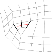
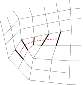
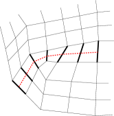
Figure 4: Construction of the parallel sets $\Pi_{k}(e)$, $k=1,\ldots,4$, indicated by bold edges. The red line connects all of them and grows in both directions.

To assess the overall run time of this algorithm, we note that in 2d, each edge has exactly two neighboring cells unless it is at the boundary, i.e., $|K(\delta)|\leq 2$. Furthermore, within each cell, there is exactly one other parallel edge to a given edge $\delta$, i.e., $|{\cal N}_{K}(\delta)|=1$. Consequently, in step (2)(b) we have $|{\cal E}(\delta)|\leq 2$ and it follows that $|\Delta_{k}|\leq 2$. With the appropriate data structures – for example, by representing sets of known maximal cardinality through fixed-sized arrays –, all operations in steps (2)(a)–(d) can then be executed in ${\cal O}(1)$ operations. Furthermore, since $\Pi_{k}(e)$ grows by one or two elements per iteration, the loop represented by step (2) executes at most $|\Pi(e)|$ times. The total cost of the algorithm is therefore ${\cal O}(|\Pi(e)|)$.

The next step is based on the realization that every edge $e$ in the graph $G_{\mathbb{T}}$ can be uniquely sorted into one of a collection of mutually exclusive sets $\pi=\{\Pi_{1},\ldots,\Pi_{N_{\Pi}}\}$. Each class $\Pi_{i}$ is constructed as above. Because the connecting line for each parallel set is either closed or ends on both sides at the boundary, the number of distinct sets of parallel edges, $|\pi|$, is at least half the number of boundary edges, but of course at most half the number of edges in $G_{\mathbb{T}}$.

Algorithmically, we can construct the collection $\pi$ of parallel sets in the following way:

Algorithm 7 ((Construct the set of parallel edge sets)).

Construct the set of parallel edge sets as follows:

1. Set $\pi=\emptyset,{\cal E}=E$.

2. While ${\cal E}\neq\emptyset$, do:

   1. Choose any $e\in{\cal E}$.

   2. Compute $\Pi=\Pi(e)$ using Algorithm 6.

   3. Set $\pi=\pi\cup\{\Pi\}$.

   4. Set ${\cal E}={\cal E}\backslash\Pi$.

Here, the set of not-yet-classified edges ${\cal E}$ is reduced one equivalence class – i.e., by one set of globally parallel edges – at a time. Because the decomposition of edges into equivalence classes is unique, it is clear that in each iteration, $\Pi\subseteq{\cal E}$. Furthermore, $\Pi(e)\supseteq\{e\}$ and so $|\Pi|\geq 1$; thus, the iteration is guaranteed to terminate.

More concretely, the cost of each iteration is given by Algorithm 6, i.e., ${\cal O}(|\Pi(e)|)$. The overall cost is therefore $\sum_{\Pi\in\pi}{\cal O}(|\Pi|)$. On the other hand, because edges can be uniquely sorted into their equivalence classes, we know that $\bigcup_{\Pi\in\pi}\Pi=E$. Thus, the cost of Algorithm 7 is ${\cal O}(|E|)$, i.e., of optimal complexity.

3.2 Orienting the elements of a set of parallel edges

Our convention was only that opposite edges in a cell have parallel directions, but there was no requirement on the relative directions of adjacent (non-opposite) edges within a cell. In fact, that was the basis for restating Conventions 1 and 2 in terms of Convention 4 and 5. It is thus easy to see that we only have to make sure that we have consistent directions of all edges within each set of parallel edges, and that consistency of edges within each such set is independent of the directions of edges in all other parallel sets. The following lemma proves that within each such equivalence class a consistent set of directions exists:

Lemma 8.

Let $e\in E$. Then there exists a choice of orientations for the elements of $\Pi(e)$ that is consistent; i.e., for all $e^{\prime},e^{\prime\prime}\in\Pi(e)$ so that $e^{\prime}\mathrel{\|_{K}}e^{\prime\prime}$ for some cell $K$, then the orientations we associate with $e^{\prime}$ and $e^{\prime\prime}$ are consistent in $K$.

This statement can be proven in a variety of ways, both constructively and in indirect ways. The most intuitive way uses the fact that a curve in the plane, closed or not and possibly self-intersecting, such as the dotted line in Fig. 4, allows for the definition of a unique direction “from one side of the curve to the other”, and we can then orient each edge it crosses according to this direction. This statement appears obvious on its face. For closed, non-intersecting curves, it follows from the Jordan Curve Theorem that states that such curves partition the plane into an “inside” and “outside” area and we can then, for example, choose the direction from the inside to the outside to orient edges. Proving the existence of such a direction field for self-intersecting curves requires more work. The history of the Jordan Curve Theorem teaches us that care is necessary, and our variations on a proof typically required a page or more of geometry, even when taking into account that we only need to show the statement for the piecewise linear curves that connect edge midpoints.

Thus, rather than providing such a proof here, let us for now simply consider the lemma to be true. A proof will later follow from Remark 11 and a statement in the appendix where we show a more general statement of which Lemma 8 is simply a special case.

Given this statement of feasibility, we can now ask for an algorithm that assigns directions to all edges in a set $\Pi(e)$ and that can be implemented with ${\cal O}(|\Pi(e)|)$ complexity. We do so by extending Algorithm 6 to include edge orientation assignment:

Algorithm 9 ((Orient edges for consistency)).

Let $\pi=\{\Pi_{1},\ldots,\Pi_{N_{\Pi}}\}$ be given. Then perform the following operations for each $i=1,\ldots,N_{\Pi}$:

1. Assign an “unassigned” orientation to each edge $e\in\Pi_{i}$.

2. Choose some $e\in\Pi_{i}$ and set $\Delta_{0}=\{e\},k=1$.

3. Assign an arbitrary orientation to $e$.

4. Set $\Delta_{k}=\emptyset$.

5. While $\Delta_{k-1}\neq\emptyset$, do:

   1. For each $\delta\in\Delta_{k-1}$:

      • Set ${\cal E}(\delta)=\emptyset$.

      • For each $K\in K(\delta)$:

        1. Set ${\cal N}_{K}(\delta):=\{\varepsilon\in e(K):\varepsilon\mathrel{\|_{K}}\delta\}\backslash\{\delta\}$.

        2. Assign an orientation to the elements of ${\cal N}_{K}(\delta)$ that is consistent in $K$ with that of $\delta$.

        3. Set ${\cal E}(\delta)={\cal E}(\delta)\cup{\cal N}_{K}(\delta)$.

      • Set $\Delta_{k}=\Delta_{k}\cup\left({\cal E}(\delta)\backslash\Pi_{k}(e))\right)$.

   2. $\Pi_{k+1}(e)=\Pi_{k}(e)\cup\Delta_{k}$.

   3. Set $k:=k+1$.

It is important to note that in step (5)(a)(ii), we assign directions only to the cell neighbors ${\cal N}_{K}(\delta)$ of $\delta$, all of which either do not yet have an orientation, or that have already been assigned that very same orientation when coming “from the other side of the parallel set” in case the connecting line for this set is a closed line through our mesh. The step therefore never changes an already assigned orientation.

The algorithm above would, in practice, simply be implemented as part of computing the parallel sets $\Pi_{i}$. In that case, it isn’t even necessary to explicitly build $\Pi_{k}(e)$ in step (5)(b) as this set is only used in the last part of step (5)(a) where we could simply exclude all elements from ${\cal E}(\delta)$ that had previously already been assigned an orientation.

3.3 Orienting all edges in a graph

With these results, we can state the main result for the case $d=2$:

Theorem 10.

For every planar, undirected graph $G_{\mathbb{T}}$ generated by subdividing a bounded domain in ${\mathbb{R}}^{2}$ into finitely many quadrilaterals, there exists a corresponding, consistently oriented directed graph $G_{\mathbb{T}}^{+}$.

Proof.

The proof follows from the preceding subsections: first, we can uniquely sort all edges into equivalence classes, for which we can choose edge directions independently; second, we can find a consistent choice of edge directions within each such set. ∎

Since both sorting edges into equivalence classes and assigning directions to edges of all equivalence classes are linear in the number of edges in the equivalence set, the overall algorithm is ${\cal O}(|E|)$ and therefore order optimal in the number of edges. Furthermore, because each edge is shared by no more than two cells and because each cell is bounded by exactly four edges, it is obvious that $\frac{1}{4}|E|\leq|{{\mathbb{T}}}|\leq 2|E|$. It follows directly that the algorithm is not only linear in the number of edges, but also in the number of cells (which is the more important estimate in practice).

Remark 11.

The arguments above showing that 2d meshes are always orientable can be carried over to meshes on two-dimensional, orientable surfaces, and we will prove so in the appendix. In particular, this holds for the practically important case of 2d meshes covering (part of) the surface of a 3d domain. Indeed, this is true whether the domain is homeomorphic to the unit ball or not – i.e., meshes on the surface of 3d domains with handles are still orientable.

The proof of this more general statement then also covers Lemma 8: the lemma states the orientability of edges of a mesh in the plane ${\mathbb{R}}^{2}$, which is obviously an orientable, two-dimensional manifold. The proof of Lemma 8 thus follows from the proof given in the appendix.

On the other hand, meshes on non-orientable surfaces, for example on a Möbius strip, are not necessarily orientable. This is because some of the connecting lines of parallel edges (see Fig. 4) may wrap around the strip and return what we thought to be a vector from “one side to the other side” in its reverse orientation. It is therefore not possible to define a unique “right” and “left” of a curve on a non-orientable manifold, and not all sets of edges of a mesh defined on it may have a consistent orientation.

Remark 12.

As mentioned in a footnote to Section 1 and Fig. 2, one can imagine other conventions for the relative orientations of edges and cell. For example, for triangles one often assumes a circular orientation. Such a convention could also be adopted for quadrilaterals. However, it has two problems: (i) It is not obvious how to generalize it to hexahedra. (ii) It is easy to construct meshes for which no set of globally consistent edge orientations can be found. To see this, note that a circular choice for edge directions in each cell implies that opposite edges have anti-parallel directions. Then imagine a closed string of $n$ cells. One of the sets of parallel edges then contains all of the $n$ edges that separate the $n$ cells forming a circle. The convention requires us to orient them alternatingly – something that is only possible if $n$ happens to be even.

4 The three-dimensional case

Let us now also look at the case of three spatial dimensions, and a subdivision of the domain into hexahedral cells. The right panel of Fig. 2 shows the convention for $d=3$, where again we will want to have all parallel edges point in the same direction. Note that now we have three sets of four edges within each cell.

We will have to investigate both whether the algorithms discussed in the previous section always yield a consistent edge orientation, and what their complexity is given the changed circumstances.

4.1 Are the edges of 3d meshes always orientable?

The first step is to construct the sets of parallel edges, $\pi$. Algorithm 6 again finds all elements of an equivalence set $\Pi(e)$ for a given starting edge $e$. Instead of following a line intersecting opposite edges starting at $e$ in both directions, we now have to follow a sheet going through all four parallel edges of a hexahedron. It is easy to see that again there is a unique classification of all edges into equivalence sets of parallel edges.

The second step was to assign a consistent orientation to the edges in a set of parallel edges. This was possible for $d=2$ since the line that connects all these edges is always orientable. However, that is not the case for the sheet connecting the edges in $d=3$: It may not be orientable, and in this case we will not be able to find a consistent orientation for the edges in this equivalence class because we can no longer choose their directions to be from “one side” to the “other side” of the sheet. The following two sections show examples of meshes whose edges are not orientable according to our conventions.

A first counterexample

. .

. .

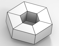
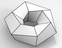
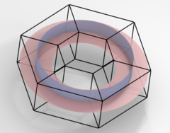
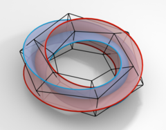
Figure 5: First counterexample for $d=3$. Taking a string of cells (top) and bending them into a torus yields a graph for which a consistent orientation of edges exists (center left). However, twisting the cells by $180^{\circ}$ before re-attaching ends fails to yield such a graph (center right): The sheets connecting the radial and axial parallel edges form two intersecting, non-orientable Möbius strips (bottom).

A first non-orientable example is shown in Fig. 5, demonstrating a subdivision of a toroidal domain for which no consistent edge orientation exists. If we take a string of cells (top) and bend it into a torus (bottom left), then all edges can be grouped into one radial, one axial, and $|{{\mathbb{T}}}|$ tangential classes (the surfaces connecting the edges of the first two classes are shown in the bottom row of Fig. 5). One possible consistent orientation would be radially inward and axially into positive $z$-direction. The tangential edges can be oriented arbitrarily for each cell separately. However, such a consistent choice of direction for edges no longer exists if we twist the string of cells by $180^{\circ}$ before attaching ends (bottom right). In that case, there must be at least one cell with radial edges that both point inward and outward, in violation of our convention. The same holds for a twist of $90^{\circ}$, in which case the sheet connecting parallel edges has to circle the torus twice, before meeting itself in the wrong orientation again. The sheet that passes through parallel edges is, in these cases, a Möbius strip with either a twist of $180^{\circ}$ or $90^{\circ}$, and it is well known that this surface is not orientable.

A second counterexample

Conjecturing from the first example that triangulations into hexahedra with no consistent orientation must have a hole or be multiply connected, is wrong, though. Fig. 6 shows an example of 14 hexahedra subdividing a simply connected domain without holes for which no consistent orientation exists. The bottom row of the figure shows the top face of the seven lower hexahedra (left) and the bottom face of the upper seven (right). Only faces $A$ and $B$ match and are connected.

. .

. .

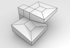
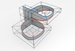
Figure 6: Second counterexample for $d=3$ with a simply connected domain. Top row: Hexahedralization and one of the sheets passing through parallel edges. Bottom row: Top face of lower half of domain and bottom face of upper part of domain, both showing consistent directions of edges if one oriented the edge $(v_{4},v_{3})$ as shown. This leads to conflicting directions for $(v_{4},v_{1})$, and the same happens if one had oriented $(v_{4},v_{3})$ in the opposite direction. Note that the two parts shown are connected only on faces $A$ and $B$.

Let us consider the orientation of the radial edges of the lower left picture: starting, for example, at edge $e$, then all radial edges must either point inward or outward due to the opposite edge rule. Also, the direction of the other two edges of face $A$ is then fixed. One of the two possibilities for directions of these edges is shown in the bottom left part of Fig. 6. Independent of these two possible choices, we have the invariant that $v_{2}$ and $v_{4}$ are vertices to which both lines in $A$ either converge, or from which they emanate, and $v_{1}$ and $v_{3}$ are vertices into which one line enters and from which one line emerges.

Now let us consider the underside of the upper seven hexahedra, given by the lower right figure. It is connected to the lower part along faces $A$ and $B$. By the same argument, starting for example at edge $e^{\prime}$, the directions of the radial edges and the other two edges of face $A$ are fixed. However, this time vertices $v_{1}$ and $v_{3}$ are the vertices from which both adjacent edges in $A$ emerge and into which they vanish, and $v_{2}$ and $v_{4}$ are the ones through which they pass, i.e. the character of the vertices is changed. Since in the joint domain vertices and edges of the upper- and undersides are identified, this creates a conflict: whatever direction we choose for edges $e$ and $e^{\prime}$, no consistent edge orientation of the face $A$ is possible.

This is easily understood by looking at the sheet that connects the set of parallel edges, $\Pi(e)=\Pi(e^{\prime})$, shown in the upper right part of the figure. It is a split, self-intersecting sheet that is not orientable.

4.2 Algorithm complexity

The examples in the previous subsection show that not all 3d meshes allow for a consistent edge orientation. In a sense, the complexity of our algorithm may therefore be a moot point: codes do necessarily have to store explicit edge orientation flags for each cell because the orientation of edges can no longer be inferred from the orientation of the cell.

On the other hand, it may still be of interest to orient edges consistently for those meshes for which this is possible, for example to ensure that the code paths for default edge orientation are always chosen. We may also be interested in seeing whether our algorithm can at least detect in optimal complexity whether a mesh is orientable.

To investigate these questions, we note that Algorithms 6 and 7 separating edges into the set $\pi$ of equivalence classes continue to work. Algorithm 6 determines the overall complexity. In 3d, we need to note that in step (2)(b)(i), ${\cal N}_{K}(\delta)$, the set of edges parallel to $\delta$ in cell $K$, now has cardinality 3. Furthermore, the loop in step (2)(b) now iterates over all cell neighbors $K(\delta)$, of which in 3d there may in fact be up to $|{{\mathbb{T}}}|$. Consequently, we can no longer bound $|{\cal E}(\delta)|$ by a constant independent of the number of edges or cells, and this then applies to the cost of the entire step (2)(b). This would not be a problem if we added at least a fixed fraction of the elements of ${\cal E}(\delta)$ to $\Delta_{k}$ (i.e., if we could guarantee that $\frac{|{\cal E}(\delta)\backslash\Pi_{k}(e)|}{|{\cal E}(\delta)|}\geq c>0$), but we are not aware of any theoretical argument that this would be so. Consequently, it is conceivable that there exist sequences of meshes for which $|{\cal E}(\delta)|={\cal O}(|E|)$ but for which step (2)(c) adds only a fixed number of elements to $\Pi_{k}$ (or at least a number that grows less quickly than $|E|$). This would destroy the linear complexity of the overall algorithm.

From a practical perspective, however, this question is not terribly interesting as it requires meshes in which the number of cells adjacent to individual edges becomes very large. While the optimal number of cells adjacent to each edge would be four (for example in a cubic lattice), practical meshes generated by mesh generators rarely have more than 8 or 10 such adjacent cells per edge, and this number is independent of the number of cells. Consequently, for such meshes, $|{\cal E}(\delta)|={\cal O}(1)$ and the algorithm is then again guaranteed to run with optimal complexity. We believe that it would also be possible to reformulate the algorithms in ways that allow for optimal complexity even for these pathological cases, though this is of no interest in the current paper.

Finally, we note that when a mesh is not orientable, step (5)(a)(ii) of Algorithm 9 will eventually try to assign a direction to an edge that already has an orientation that is inconsistent with the one that we want to assign to it (a case that cannot happen in 2d). Thus, the algorithm will be able to detect non-orientable meshes with the same run time complexity as it can orient meshes.

5 Meshes in $d=3$ that are always orientable

The fact that not all 3d meshes can be consistently oriented of course does not rule out that there may be important subclasses of 3d meshes that can in fact be oriented. Indeed, we will show these statements in the following subsections:

1. Refining a non-orientable mesh uniformly yields a mesh that is consistently orientable.

2. Three-dimensional meshes generated by extruding a two-dimensional mesh into a third direction are always orientable.

3. Hexahedral meshes that result from subdividing each tetrahedron of a tetrahedral mesh into hexahedra are always orientable.

We will discuss these three cases in the following.

5.1 Meshes originating from refinement of non-orientable meshes

If one is given a three-dimensional mesh with a sheet of parallel edges that are not consistently orientable, then it turns out that we can generate an orientable mesh by subdividing all the cells along this sheet. To understand this intuitively, remember that a non-orientable surface somehow connects to itself “with a twist of $180^{\circ}$”. If we refine all the cells along its way, we duplicate this sheet and replace it by one that “goes around twice before connecting to itself again”. The twist is thus $360^{\circ}$ and the resulting sheet is orientable. This is illustrated in Fig. 7 for the two examples discussed in Section 4.1.

.

.

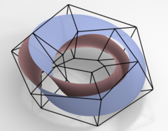
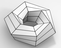
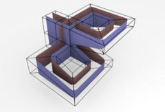
Figure 7: Illustration that splitting a non-orientable sheet by subdividing each edge along the sheet into two, yields a single orientable sheet. Top left: The sheet that results from subdividing one of the two Möbius strips in Fig. 5. Top right: The mesh one obtains by refining all edges along both of the non-orientable sheets in Fig. 5. This mesh is orientable. Bottom: The same for the example shown in Fig. 6.

To make this more formal, let us consider an equivalence class $\Pi_{G_{\mathbb{T}}}(e)$ of parallel edges which is not consistently orientable. Here, we use the index to indicate that this is a set of edges in the graph $G_{\mathbb{T}}$. Now split each cell that the sheet associated with $\Pi_{G_{\mathbb{T}}}(e)$ intersects, into 2, 4, or 8 new cells (depending on whether the sheet intersects the cell once, twice, or three times, i.e., whether one, two, or all three of the sets of parallel edges within this cell are part of $\Pi_{G_{\mathbb{T}}}(e)$). We subdivide in the directions orthogonal to the sheet, see Figure 8. This removes the affected edges from the graph, and replaces them by 8, 24, or 54 new “child” edges. With this refined mesh is associated a new graph $G^{\prime}$. Then the following results hold:

. .

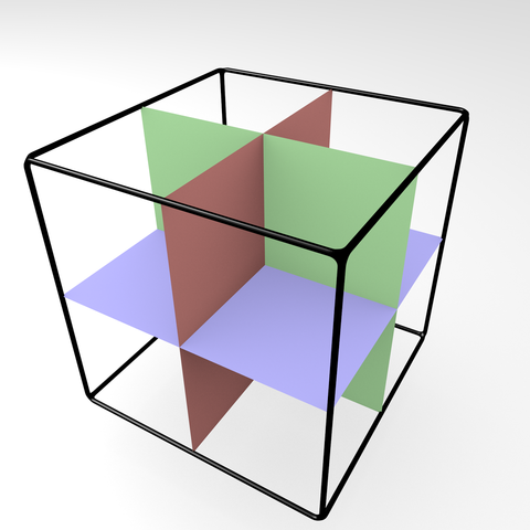
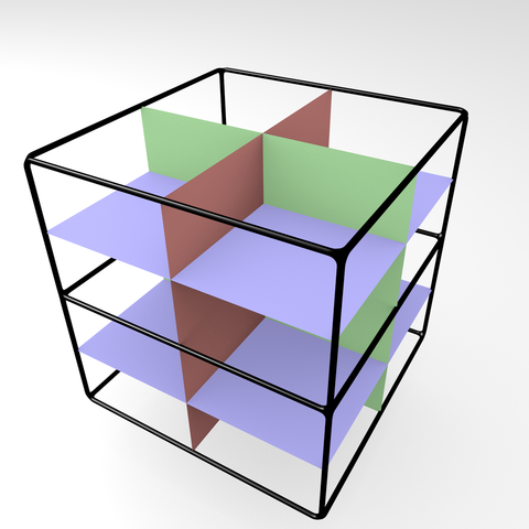
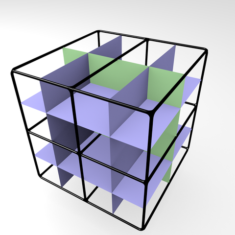
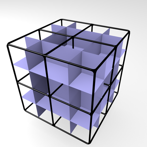
Figure 8: Illustration of splitting a cell (left) along the purple connecting sheet (left center), as well as along the purple sheet in cases where it runs through the same cell twice (center right) or three times (right).

Lemma 13.

Let $\Pi_{G_{\mathbb{T}}}(e)$ be a set of parallel edges that are not consistently orientable, and $\Pi_{G^{\prime}}(e^{\prime})$, $\Pi_{G^{\prime}}(e^{\prime\prime})$ the sets of parallel edges in the refined graph $G^{\prime}$ associated with the “children” $e^{\prime},e^{\prime\prime}$ of $e$. Then $\Pi_{G^{\prime}}(e^{\prime})=\Pi_{G^{\prime}}(e^{\prime\prime})=:\Pi$. Furthermore, $\Pi$ is orientable.

Proof.

By refining each cell with edges in $\Pi_{G_{\mathbb{T}}}(e)$ along the non-orientable sheet, we replace each edge $\varepsilon_{i}\in\Pi_{G_{\mathbb{T}}}(e)$ by two edges $\varepsilon_{i}^{\prime},\varepsilon_{i}^{\prime\prime}$. Let us select an arbitrarily chosen element from $\Pi_{G_{\mathbb{T}}}(e)$, and denote it for simplicity by the symbol $e$. Its children, after refinement, $e^{\prime},e^{\prime\prime}$ are edges in the refined graph $G^{\prime}$, and their respective sets of parallel edges are $\Pi_{G^{\prime}}(e^{\prime}),\Pi_{G^{\prime}}(e^{\prime\prime})$. It is easy to see that each of the two children $\varepsilon^{\prime},\varepsilon^{\prime\prime}$ of each edge $\varepsilon\in\Pi_{G_{\mathbb{T}}}(e)$ must be in either $\Pi_{G^{\prime}}(e^{\prime})$ or $\Pi_{G^{\prime}}(e^{\prime\prime})$.

We first show that these sets are equal. Assume that $\Pi_{G^{\prime}}(e^{\prime})\neq\Pi_{G^{\prime}}(e^{\prime\prime})$. Then we could find a unique direction for each edge $\varepsilon\in\Pi_{G_{\mathbb{T}}}(e)$ by assigning it the direction “from the $\Pi_{G^{\prime}}(e^{\prime})$ side to the $\Pi_{G^{\prime}}(e^{\prime\prime})$ side.” This, however, would be a consistent orientation of the edges in $\Pi_{G_{\mathbb{T}}}(e)$, in contradiction to the assumption that this set is non-orientable. Thus, $\Pi_{G^{\prime}}(e^{\prime})=\Pi_{G^{\prime}}(e^{\prime\prime})$. Intuitively, this means that splitting the single sheet associated with $\Pi_{G_{\mathbb{T}}}(e)$ still yields a single sheet.

The second step is to show that the single set $\Pi=\Pi_{G^{\prime}}(e^{\prime})=\Pi_{G^{\prime}}(e^{\prime\prime})$ is orientable. We do this purely locally: choose for the two children $\varepsilon^{\prime},\varepsilon^{\prime\prime}$ of an edge $\varepsilon\in\Pi_{G_{\mathbb{T}}}(e)$ the direction away from their common node (“centrifugal direction”: the direction vectors of the child edges are “rooted” in the original sheet through $\Pi_{G_{\mathbb{T}}}(e)$). This orientation of the children of $\Pi_{G_{\mathbb{T}}}(e)$ is consistent with our convention for every one of the affected child cells, and, consequently, for all cells which the sheet for $\Pi_{G_{\mathbb{T}}}(e)$ intersects. Intuitively, this can be interpreted as follows: while the sheet has no associated normal direction, the direction “away from the sheet” exists on both sides. ∎

As can be seen in Fig. 8, refinement of a cell along one sheet also adds new edges to other sets of parallel edges. Depending on whether the sheet intersects a cell once, twice, or three times, refinement adds 4, 5, or no new edges to other parallel sets. However, we can show that refining the cells along one non-orientable sheet does not render a previously orientable, other sheet non-orientable:

Lemma 14.

Let $\Pi_{G_{\mathbb{T}}}(e)$ be a set of parallel edges that are refined to make it orientable. Let $\Pi_{G_{\mathbb{T}}}(e^{\prime})$ be a set of parallel edges to which edges are added by this refinement step. Then, if $\Pi_{G_{\mathbb{T}}}(e^{\prime})$ was orientable before the refinement step, then it is also after the refinement step.

Proof.

If the edges in $\Pi_{G_{\mathbb{T}}}(e^{\prime})$ were already orientable in $G_{\mathbb{T}}$, then they must have parallel directions in the cell shown in Fig. 8. If we assign the same, parallel direction to the newly added edges in $G^{\prime}$ that belong to this set of parallel edges in $G^{\prime}$, then the resulting directions are consistent in the child cells as well. Because the remainder of the cells intersected by $\Pi_{G_{\mathbb{T}}}(e^{\prime})$ are not affected, the locally consistent edge orientations in the child cells implies that $\Pi_{G^{\prime}}(e^{\prime})$ remains orientable.

On the other hand, if $\Pi_{G_{\mathbb{T}}}(e^{\prime})$ was not orientable, then this fact is unaltered by the addition of new edges. ∎

With these lemmas, we can state the final result of this section:

Theorem 15.

Let $G_{\mathbb{T}}$ be the graph associated with a subdivision of a domain into hexahedra. If it is not orientable, then we can generate a new graph $G^{\prime}$ by refining all cells exactly once along the sheets associated with those sets of parallel edges that are not orientable.

Proof.

The theorem follows from the previous two lemmas. As was shown in Lemma 13, we can convert a non-orientable set of parallel edges into an orientable one. In Lemma 14, we showed that this does not create new non-orientable sets. Since the original graph can only have finitely many non-orientable sets of parallel edges, we decrease this number by one in each refinement step and thus obtain an orientable graph in a finite number of steps. ∎

Thus, even though there are three-dimensional meshes that cannot be oriented according to our convention, above theorem shows that there is a simple and inexpensive remedy for these cases. While the meshes resulting from such anisotropic refinement have a worse aspect ratio, one can simply refine all hexahedra uniformly into eight children to obtain an orientable mesh with the same aspect ratio of cells as the original one. This corresponds to refining the cells intersected by all sheets associated with sets of parallel edges, not only those corresponding to non-orientable ones. Obviously, this mesh is also orientable: in addition to the originally non-orientable parallel sets, we now also refine the originally orientable parallel sets, which yields two distinct sets of parallel edges $\Pi_{G^{\prime}}(e^{\prime})$ and $\Pi_{G^{\prime}}(e^{\prime\prime})$ that can independently be oriented, one on “this” side of the original sheet and one on “that” side of it (these sides are distinct because the sheet associated with $\Pi_{G_{\mathbb{T}}}(e)$ was orientable).

Remark 16.

The observations of this section also point out an important optimization in practice for codes that create finer meshes by subdividing the cells of an existing mesh. In such cases, it is not necessary to re-run the mesh orientation algorithm on the finer mesh with four (2d) or eight (3d) times as many cells. Rather, if the original mesh was already consistently oriented, then the new mesh will be consistently oriented by simply choosing the directions of the refined edges to be the same as those of their parent edge.

5.2 Extruded meshes

An important class of meshes consists of those that start with a two-dimensional quadrilateral mesh and then “extrude” it into a third direction by replicating it one or more times and connecting the vertices of the original mesh and its replicas in this third direction. Indeed, the mesh shown at the top of Fig. 5 is such a mesh: the sequence of quadrilaterals at the bottom has been replicated to the top, and each pair of original and replicated vertices are connected by a new edge.

Extruded meshes are often used for “thin” domains. The technique is obviously also applicable if the original two-dimensional mesh lived on an (orientable) manifold such as the bottom surface of the object we want to mesh. The extrusion also need not necessarily be in a perpendicular direction, nor do the replicas have to be parallel to the original mesh. That said, for the purposes of orienting edges, such geometric considerations are immaterial.

For extruded meshes, we can state the following result:

Theorem 17.

Let $\{K\}$ be a hexahedral mesh obtained by extruding a quadrilateral mesh defined on a two-dimensional, orientable manifold in a third direction. Then the edges of this mesh are consistently orientable.

Proof.

To understand why this is the case, recall that all two-dimensional quadrilateral meshes on such manifolds are orientable. In other words, in the original mesh, opposite edges can already be chosen to be parallel, and this is also the case for its replicas.

Next, consider the sets of parallel edges we may consider. Obviously, the edges of the original mesh and its replicas are parallel, and we can consistently orient them if we choose edge directions of the original mesh and its replicas the same. An alternative viewpoint is that the sheets that connects these sets of parallel edges are the “extruded” version of the line that connected these parallel edges in the two-dimensional mesh, and the orientability of the one-dimensional line then extends to the orientability of the corresponding sheet to which it gives rise.

The only additional sets of parallel edges are the ones that connect the original mesh and its first replica, and then each replica with the next. The corresponding sheets can be thought of as copies of the two-dimensional domain spanned by the original mesh, located halfway between the replicas. Each of these sheets is obviously orientable: The edges of each of these new sets are independent of each other, and each class can be consistently oriented, for example by always choosing the direction from the original to the first replica, and from each replica to the next (i.e., an “upward” direction). ∎

5.3 Meshes originating from tetrahedralizations

The examples in Section 4.1 show that there is no topological characterization of those domains for which we can always find a consistent orientation of edges. Rather, it is a question of how that domain was subdivided into cells. Indeed, we can show that for the very general class of domains that can be subdivided into tetrahedra, there also exists a subdivision into hexahedra with a consistent orientation of edges:

Theorem 18.

Let $\{T\}$ be a given subdivision of a domain $\Omega$ into a set of tetrahedra so that two distinct tetrahedra either have no intersection, share a common vertex, a complete edge, or a complete face. Divide each tetrahedron $T$ into four hexahedra, $K(T)_{0},\ldots,K(T)_{3}$, by using the vertices, edge midpoints, face midpoints, and cell midpoint of $T$ as vertices for the hexahedra. Then the edges of the mesh consisting of the union of these hexahedra, $\bigcup_{T,0\leq i<4}K_{i}(T)$, are consistently orientable.

Before we prove this claim, we note that the resulting hexahedra are in almost all cases not close to the optimal cube shape. Also, almost all vertices in the resulting mesh have a number of cells meeting at this vertex that deviates from the optimal number of eight (encountered, for example, in a regular subdivision into cubes). These meshes are therefore hardly optimal for finite element computations. However, given the complexity of generating hexahedral meshes, until recently many mesh generators used this approach to generate an initial hexahedral mesh. (For example, the widely used open source mesh generator gmsh [8] can use this approach to generate hexahedral meshes.)

. .

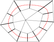
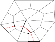
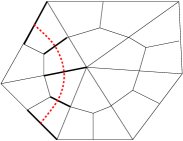
Figure 9: Construction in $d=2$ for the proof of Theorem 18. Top: Part of a subdivision into triangles before and after cutting each triangle into three quadrilaterals (top row). Bottom: Three sets of parallel edges and their connecting line (bottom row).

of Theorem 18.

In order to explain the proof in $d=3$, it is instructive to first consider a similar case in $d=2$, where we would cut all cells of a triangular mesh into three quadrilaterals, see Fig. 9. From the edges of these quadrilaterals, we then generate independent sets of parallel edges; the bottom row of the figure shows three of these sets along with their connecting line.

Importantly, each of these lines forms a closed, non-self-intersecting loop around one of the original vertices of the triangles, cutting through all the cells in the second layer of quadrilaterals around this vertex (unless, of course, the vertex is at the boundary of the domain, in which case the line is not closed but starts and ends at the boundary). Indeed, the edges of each quadrilateral are part of the loops for two vertices of the triangle from which it arose. Each vertex thus gives rise to at least one set of parallel edges in the subdivision into quadrilaterals. These can, of course, all be oriented in $d=2$. (It may give rise to more than one such set if two parts of the domain touch at a vertex, i.e., if there are two sets of cells adjacent to a vertex that are not mutual face neighbors.)

It is easy to generalize these considerations to the case $d=3$ (though we have not found good ways to visualize hexahedral meshes resulting from even a small collection of tetrahedra forming an unstructured mesh). First, we note that each original interior vertex now induces a set of parallel edges that is connected by a closed non-self-intersecting sheet around the vertex. Since it is homeomorphic to the surface of the unit sphere, it is of course orientable, and so are the edges of this parallel set. For original vertices on the boundary, the sheet is not closed, but it is obviously still orientable. ∎

6 Conclusions

Finite element codes can be made significantly simpler if they can make assumptions about the relative orientations of coordinate systems defined on cells, edges, and faces. If such assumptions always hold, then this reduces the number of cases one has to implement and, consequently, the potential for bugs. In this paper, we have described a way to orient edges and the cells they bound, and shown that not only is it possible to choose edge directions consistently with regard to this convention for two-dimensional quadrilateral meshes, but also that there is an efficient algorithm to find such edge orientations.

On the other hand, it is not always possible to orient edges of three-dimensional hexahedral meshes according to the three dimensional generalization of this convention. The obvious generalization of our two-dimensional algorithm is able to detect these cases, again in optimal complexity, but the result implies that codes dealing with hexahedral meshes necessarily have to store flags for each of the edges of each cell that indicate the orientation of that edge relative to the coordinate system of the cell. This is not a significant overhead in terms of memory and possibly not in terms of algorithmic complexity. Nevertheless, in actual practice, this has turned out to be an endless source of frustration and bugs in deal.II as the cases where edge orientations are relevant are restricted to the use of higher order elements, as well as complex and three-dimensional geometries. In case of bugs, methods generally converge but at suboptimal orders. Consequently, debugging such cases and detecting where in the interplay of geometry, mappings, degrees of freedoms, shape functions, and quadrature the bug resides has proven to be a very significant challenge. This experience also supports our claim that being able to enforce a convention in the two-dimensional case almost certainly saved a great deal of development time.

At the same time, this paper at least identifies broad classes of three-dimensional meshes for which one can always consistently orient edges, and for which no special treatment of edges is necessary. Through counter-examples, we have shown that there is no topological description for which domains do or do not allow for consistent orientations, but that it is indeed a property of how the domain is subdivided into cells, and our analysis demonstrates ways by which meshes can be constructed in ways so that edges can always be oriented consistently. This analysis can therefore also provide constructive feedback for the design of mesh generation algorithms.

Acknowledgments

WB would like to thank J. M. Landsberg, J.-L. Guermond, and A. Ern for illuminating discussions.

Appendix A Quadrilateral meshes on two-dimensional manifolds

Lemma 8 provided the basis for the proof that we can find consistent orientations of the edges for all meshes that subdivide a domain $\Omega\subset{\mathbb{R}}^{2}$ into quadrilaterals. Fundamentally, the reason for its truth is the geometric fact that the piecewise linear curve connecting a set of parallel edges has a unique “left” and “right” side.

As mentioned in Remark 11, this can be generalized to the connecting lines on orientable, two-dimensional manifolds. Geometric proofs for this extension are complicated by two facts: (i) the underlying manifold may not be smooth, for example in the case of a mesh on the surface of a body with edges and corners (such as a cube); (ii) we need to be careful how exactly we embed the curve connecting parallel edges into the manifold. Consequently, it is easier to avoid the language of geometry altogether. Rather, we will use the language of combinatorial topology that in its essence only uses what we are given: the quadrilateral mesh.

In the statement of the following result, we will use the combinatorial topology definition of what an “orientable” manifolds is (see [14, 16] and below). This class of manifolds includes all smooth two-dimensional manifolds that are orientable in the differential geometry sense [19], but also (parts of) the boundaries of domains in ${\mathbb{R}}^{3}$ [6, Chapter VI, Theorem 7.15]. Furthermore, the manifolds we can consider need not be naturally embedded in ${\mathbb{R}}^{3}$. A special case of an orientable, two-dimensional manifold is of course the plane ${\mathbb{R}}^{2}$, covering the situation of Lemma 8. Then the following is true:

Theorem 19.

Let ${\mathbb{T}}$ be a quadrilateral mesh with finitely many cells on an arbitrary, two-dimensional, orientable manifold, and $G_{\mathbb{T}}$ the associated graph. Then there exists a corresponding directed graph $G_{\mathbb{T}}^{+}$ that is consistently oriented.

Proof.

The proof is in essence analogous to that of Theorem 10. The only piece that has changed is that we need to provide for the orientability of edges in each of the parallel sets, i.e., the extension of Lemma 8 to orientable, two-dimensional manifolds.

To this end, let us construct a subdivision $\Delta$ of ${\mathbb{T}}$ into 2-simplices (triangles) by adding to each quadrilateral one of the two diagonals. $\Delta$ is then a simplicial 2-complex. A 2-complex is called coherently oriented if (i) the edges of each 2-simplex are either oriented clockwise or counterclockwise, and (ii) whenever two 2-simplices share a common edge, the relative orientations of this shared edge are complementary (i.e., opposing), see for example [14, Chapter 5]. A 2-manifold is called orientable if every 2-complex on it can be coherently oriented. Thus, since $\Delta$ is a 2-complex on a surface for which we have previously assumed that it is orientable, we may choose a coherent orientation of all edges of $\Delta$. Given the subdivision of each cell $K\in{\mathbb{T}}$ into two triangles with edges oriented either clockwise or counterclockwise, this induces an orientation on ${\mathbb{T}}$ where (i) opposite edges in each cell $K$ are oriented complementarily, and (ii) shared edges of two adjacent cells are oriented complementarily. One quickly checks that this is independent of the choice of diagonals.

We have previously seen that each edge $e$ is part of at most two cells and has therefore at most two opposite edges. For each set of parallel edges, $\Pi_{i}\in\pi$, there is then a sequence of cells connected by the edges $\Pi_{i}$ that is either open or that forms a closed loop. This is illustrated in Fig. 10. (Cells may occur more than once in this sequence, but only once for each pair of opposite edges in this cell.)

. .

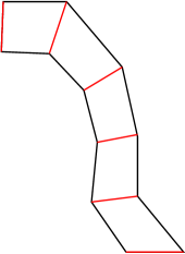
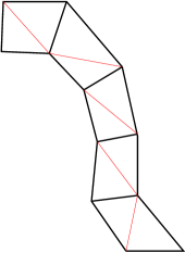
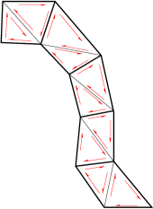
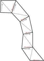
Figure 10: Construction of consistent edge orientations via simplicial complexes. Left: The part of a mesh consisting of the cells adjacent to the edges (marked in red) that form one set of parallel edges. Center left: One possible subdivision of quadrilateral cells into triangles by adding a diagonal to each cell. The result is a simplicial complex $\Delta$. Center right: Because the mesh exists on a 2-manifold that is orientable, it is possible to assign clockwise and counter-clockwise orientations to all triangles so that they imply complementary directions for each shared edge. Right: Choosing every other direction for edges between cells, as we walk along the sequence of cells, yields a set of consistent edge orientations, i.e., opposite edges in quadrilaterals are oriented in a parallel direction.

Now let us choose an edge $e\in\Pi_{i}$, and let $K$ be one (of possibly two) neighboring cell of $e$. If the sequence of cells connected by $\Pi_{i}$ is open, then assign to $e$ the direction of this edge as defined in $K$. The edge $e^{\prime}$ opposite of $e$ in $K$ is then assigned the direction defined in the neighbor of $K$ beyond $e^{\prime}$, and so forth in both directions starting at $e$. It is easy to see that this leads to a consistently oriented set of edges in the sense discussed in Section 3.

If the sequence of cells connected by $\Pi_{i}$ is closed, we need to ensure that this does not lead to a conflict. If we follow the sequence of cells, the previous construction chooses every second encountered edge orientation; because each orientation is complementary to the previous, choosing every other one leads to a consistent set of edge orientations.

We then repeat this for all classes $\Pi_{i}\in\pi$, thus finishing the proof. ∎

References

- [1] M. Ainsworth and J. Coyle. Hierarchic finite element bases on unstructured tetrahedral meshes. International Journal for Numerical Methods in Engineering, 58:2103–2130, 2003.
- [2] W. Bangerth, R. Hartmann, and G. Kanschat. deal.II – a general purpose object oriented finite element library. ACM Trans. Math. Softw., 33(4), 2007.
- [3] W. Bangerth, T. Heister, L. Heltai, G. Kanschat, M. Kronbichler, M. Maier, B. Turcksin, and T. D. Young. The deal.II library, version 8.2. Archive of Numerical Software, 3, 2015.
- [4] P. Bastian, M. Blatt, A. Dedner, C. Engwer, R. Klöfkorn, R. Kornhuber, M. Ohlberger, and O. Sander. A generic grid interface for parallel and adaptive scientific computing. Part II: implementation and tests in DUNE. Computing, 82:121–138, 2008.
- [5] E. Bertolazzi and G. Manzini. Algorithm 817: P2MESH: Generic object-oriented interface between 2-d unstructured meshes and FEM/FVM-based PDE solvers. ACM Trans. Math. Softw., 28(1):101–132, Mar. 2002.
- [6] G. E. Bredon. Topology and Geometry, volume 139 of Graduate Texts in Mathematics. Springer, 1993.
- [7] C. D. Cantwell, D. Moxey, A. Comerford, A. Bolis, G. Rocco, G. Mengaldo, D. D. Grazia, S. Yakovlev, J.-E. Lombard, D. Ekelschot, B. Jordi, H. Xu, Y. Mohamied, C. Eskilsson, B. Nelson, P. Vos, C. Biotto, R. M. Kirby, and S. J. Sherwin. Nektar++: An open-source spectral/hp element framework. Computer Physics Communications, 192:205–219, 2015.
- [8] C. Geuzaine and J.-F. Remacle. Gmsh: a three-dimensional finite element mesh generator with built-in pre- and post-processing facilities. International Journal for Numerical Methods in Engineering, 79:1309–1331, 2009.
- [9] F. Haglund and D. T. Wise. Special cube complexes. Geometric and Functional Analysis, 17:1551–1620, 2008.
- [10] G. Hetyei. On the Stanley ring of a cubical complex. Discr. Comput. Geometry, 14:305–330, 1995.
- [11] M. Homolya and D. A. Ham. A parallel edge orientation algorithm for quadrilateral meshes. arXiv, 1505.03357, 2015.
- [12] B. Kirk, J. W. Peterson, R. H. Stogner, and G. F. Carey. libMesh: A C++ Library for Parallel Adaptive Mesh Refinement/Coarsening Simulations. Engineering with Computers, 22(3–4):237–254, 2006.
- [13] A. G. Kurosh. Lectures on General Algebra. Chelsea Publishing Co., 1963.
- [14] J. Lee. Introduction to Topological Manifolds. Number 202 in Graduate Texts in Mathematics. Springer, 2nd edition, 2011.
- [15] R. Lidl and G. Pilz. Applied Abstract Algebra. Springer, New York, Berlin, Heidelberg, 2 edition, 1998.
- [16] J. Munkres. Elements of Algebraic Topology. Westview Press, 1996.
- [17] M. E. Rognes, R. C. Kirby, and A. Logg. Efficient assembly of and conforming finite elements. SIAM J. Sci. Comput., 31:4130––4151, 2009.
- [18] A. Schwartz and G. M. Ziegler. Construction techniques for cubical complexes, odd cubical 4-polytopes, and prescribed dual manifolds. Experimental Math., 13:385–413, 2004.
- [19] M. Spivak. Calculus on Manifolds. Perseus Books, 1965.
- [20] D. Teleaga and J. Lang. Numerically solving Maxwell’s equations. implementation issues for magnetoquasistatics in KARDOS. Technical report, TU Darmstadt, 2008.
- [21] S. Zaglmayr. High order finite element methods for electromagnetic field computation. PhD thesis, Johannes Kepler University, Linz, Austria, 2006.