Instability of nonminimally coupled scalar fields in the spacetime of thin charged shells

Abstract

We investigate the stability of a free scalar field nonminimally coupled to gravity under linear perturbations in the spacetime of a charged spherical shell. Our analysis is performed in the context of quantum field theory in curved spacetimes. This paper completes previous analyses which considered the exponential enhancement of vacuum fluctuations in the spacetime of massive shells.

I Introduction

It has been shown that well-behaved spacetimes are able to induce an exponential enhancement of the vacuum fluctuations of some nonminimally coupled free scalar fields lv . This “vacuum awakening effect” may be seen as the quantum counterpart of the classical instability experienced by these fields under linear perturbations mmv . The exponential growth of the vacuum energy density of an unstable scalar field in the spacetime of, e.g., a neutron star lmv would necessarily induce the system to evolve into a new equilibrium configuration culminating in the emission of a burst of free scalar particles llmv (see also Refs. novak98 ; pcbrs11 ; rdans12 for related classical analyses). Conversely, the determination of the mass-radius ratio of observed neutron stars may be used to rule out the existence of whole classes of nonminimally coupled scalar fields m ; pl . This has motivated us to investigate how the vacuum awakening effect is impacted by relaxing some symmetries assumed in Ref. lmv . In order to avoid complications in modeling the fluid, the analyses of deviations from sphericity lmmv and staticity mmv2 were considered in the context of massive thin shells. In this paper, we investigate the vacuum awakening mechanism when we endow a spherical shell with electrical charge. The presence of charge affects both the energy conditions satisfied by the shell matter and the effective potential appearing in the radial part of the scalar field equation. Hence, it is interesting to inquire how previous results for massive thin shells are modified in the charged case.

The paper is organized as follows. In Sec. II, we introduce the spacetime of a massive charged shell. In Sec. III, we quantize the real scalar field in this background and discuss the vacuum awakening effect. In Sec. IV, we investigate the exponential growth of the vacuum energy density. Section V is dedicated to our final remarks. We assume metric signature $(-+++)$ and natural units in which $c=\hbar=G=1$ unless stated otherwise.

II Spherically symmetric charged shells

Let us write the line element describing the spacetime of a spherically symmetric thin shell with mass $M$ and electric charge $Q$ lying at the radial coordinate $r=\mathsf{R}$ as b

$$ds^{2}_{-}=-f(\mathsf{R})dt^{2}+dr^{2}+r^{2}\left(d\theta^{2}+\sin^{2}\theta d\varphi^{2}\right)$$ (1)

and

$$ds^{2}_{+}=-f(r)dt^{2}+f(r)^{-1}dr^{2}+r^{2}\left(d\theta^{2}+\sin^{2}\theta d\varphi^{2}\right)$$ (2)

with

$$f(r)\equiv(1-2M/r+Q^{2}/r^{2})>0,$$ (3)

where $\mathsf{R}>M+\sqrt{M^{2}-Q^{2}}$ when $|Q|\leq M$ (while $\mathsf{R}$ may assume any positive value when $|Q|>M$) and $\mp$ labels quantities defined at $r\lessgtr\mathsf{R}$, respectively. The three-dimensional timelike surface $\cal{S}$ defined at $r=\mathsf{R}$ will be covered with coordinates $\zeta^{a}=(t,\theta,\varphi)$. The metrics $h_{ab}^{-}$ and $h_{ab}^{+}$ on $\cal{S}$ as induced from the internal- and external-to-the-shell spacetime portions, respectively, satisfy $h_{ab}^{-}=h_{ab}^{+}$ as demanded by the continuity condition.

The shell stress-energy-momentum tensor

$$T^{\mu\nu}=S^{ab}e^{\mu}_{a}e^{\nu}_{b}\delta(\ell)$$ (4)

can be computed from the discontinuity of the extrinsic curvature $\Delta K^{ab}\equiv K^{ab}_{+}-K^{ab}_{-}$ across $\cal{S}$ (see, e.g., Ref. poisson ). In Eq. (4),

$$S^{ab}\equiv-\frac{1}{8\pi}(\Delta K^{ab}-h^{ab}\Delta K),$$ (5)

where $\Delta K\equiv\Delta K_{ab}h^{ab}$, $e_{a}^{\mu}\equiv\partial x^{\mu}/\partial\zeta^{a}$ are the components of the coordinate vectors $\partial/\partial\zeta^{a}$ defined on $\cal{S}$, and $\ell$ (inside the delta distribution) is the proper distance along geodesics intercepting orthogonally $\cal{S}$ (with $\ell<0$, $\ell=0$, and $\ell>0$ inside, on, and outside $\cal{S}$, respectively). By using Eqs. (1) and (2), we obtain

$$S_{\;\;0}^{0}=\frac{1}{4\pi\mathsf{R}}\left(f(\mathsf{R})^{1/2}-1\right)$$ (6)

and

$$S_{\;\;2}^{2}=S_{\;\;3}^{3}=\frac{1}{8\pi\mathsf{R}}\left[\left(1-\frac{M}{\mathsf{R}}\right)f(\mathsf{R})^{-1/2}-1\right].$$ (7)

In order to unveil the most realistic shell configurations, we have investigated the behavior of the different energy conditions with respect to the shell parameters $\mathsf{R}/M$ and $Q/M$. (For the stability of charged shells under linear perturbations, see Ref. es .) We can see that the weak, strong, and dominant energy conditions are simultaneously satisfied in a large portion of Fig. 1, namely, region 3.

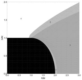
Figure 1: The graph shows where the different energy conditions are satisfied as functions of the shell parameters $\mathsf{R}/M$ and $Q/M$ out of the black area. The black area is excluded because there are no static shell configurations in this region. The weak energy condition is satisfied everywhere but in region 4. The strong energy condition is violated in regions 2 and 4, while the dominant energy condition is violated in regions 1 and 4. We see, thus, that in a large portion, namely, region 3, the three energy conditions are satisfied.

III Quantizing the field and awaking the vacuum

Now, we consider a nonminimally coupled massless real scalar field $\Phi$ satisfying the Klein-Gordon equation

$$-\nabla_{\mu}\nabla^{\mu}\Phi+\xi R\Phi=0$$ (8)

in the spacetime of our spherically symmetric charged shell, where $\xi\in\mathbb{R}$ and $R$ is the scalar curvature. We follow the canonical procedure and expand the corresponding field operator fulling ; wald_qftcs

$$\hat{\Phi}=\int d\vartheta(\eta)[\hat{a}_{\eta}u_{\eta}+\hat{a}_{\eta}^{\dagger}u_{\eta}^{*}],$$ (9)

in terms of positive, $u_{\eta}$, and negative, $u_{\eta}^{*}$, norm modes with respect to the Klein-Gordon inner product, where $\vartheta$ is a measure defined on the set of quantum numbers $\eta$. The annihilation $\hat{a}_{\eta}$ and creation $\hat{a}_{\eta}^{\dagger}$ operators satisfy $[\hat{a}_{\alpha},\hat{a}_{\beta}^{\dagger}]=\delta(\alpha,\beta)$ and $[\hat{a}_{\alpha},\hat{a}_{\beta}]=0$, where the delta function is defined by $\int d\vartheta(\alpha)\delta(\alpha,\beta)\mathcal{F}(\alpha)=\mathcal{F}(\beta)$ for $\mathcal{F}\in C^{\infty}$, and the vacuum state $|0\rangle$ must satisfy $\hat{a}_{\eta}|0\rangle=0$ for all $\eta$.

The spacetime symmetries drive us to look for positive-norm modes in the form

$$u^{\mp}_{\sigma l\mu}(t,r,\theta,\varphi)=T_{\sigma}(t)F^{\mp}_{\sigma l}(r)Y_{l\mu}(\theta,\varphi),$$ (10)

where $Y_{l\mu}(\theta,\varphi)$ represent the spherical harmonic functions, $l=0,1,2\ldots$, $\mu=-l,-l+1,\ldots l$, $\sigma={\rm const}\in\mathbb{R}$, and

$$i\left(T^{*}_{\sigma}\frac{dT_{\sigma}}{dt}-T_{\sigma}\frac{dT^{*}_{\sigma}}{dt}\right)>0$$ (11)

(positive-norm condition). By using Eq. (10) in Eq. (8), we obtain that $F^{\mp}_{\sigma l}(r)$ and $T_{\sigma}(t)$ satisfy

$$-\frac{f(\mathsf{R})}{r^{2}}\frac{d}{dr}\left(r^{2}\frac{dF^{-}_{\sigma l}}{dr}\right)+\frac{f(\mathsf{R})}{r^{2}}l(l+1)F^{-}_{\sigma l}=\sigma F^{-}_{\sigma l},$$ (12)

$$-\frac{f(r)}{r^{2}}\frac{d}{dr}\left(r^{2}f(r)\frac{dF^{+}_{\sigma l}}{dr}\right)+\frac{f(r)}{r^{2}}l(l+1)F^{+}_{\sigma l}=\sigma F^{+}_{\sigma l},$$ (13)

and

$$\frac{d^{2}}{dt^{2}}T_{\sigma}+\sigma T_{\sigma}=0.$$ (14)

Depending on the sign of $\sigma$, Eq. (14) supplemented by condition (11) admits two kinds of general solutions:

$$T_{\sigma}(t)\stackrel{{\scriptstyle\sigma=\omega^{2}}}{{\propto}}\exp(-i\omega t),\;\;\;\omega>0,$$ (15)

for $\sigma\equiv\omega^{2}>0$ and

$$T_{\sigma}(t)\stackrel{{\scriptstyle\sigma=-\Omega^{2}}}{{\propto}}e^{\Omega t-i\pi/12}+e^{-\Omega t+i\pi/12},\;\;\;\Omega>0,$$ (16)

for $\sigma\equiv-\Omega^{2}<0$. The combination chosen on the right-hand side of Eq. (16) guarantees that the corresponding $u^{\mp}_{\sigma l\mu}$ functions will be indeed positive-norm modes lv . The modes (10) with $T_{\sigma}(t)$ as given by Eqs. (15) and (16) will be denoted as

$$u^{\mp}_{\sigma l\mu}\stackrel{{\scriptstyle\sigma=\omega^{2}}}{{\longrightarrow}}v^{\mp}_{\omega l\mu}=\frac{\psi^{\mp}_{\omega l}(r)}{r}Y_{l\mu}(\theta,\varphi)\frac{\exp(-i\omega t)}{\sqrt{2\omega}}$$ (17)

and

$$u^{\mp}_{\sigma l\mu}\stackrel{{\scriptstyle\sigma=-\Omega^{2}}}{{\longrightarrow}}w^{\mp}_{\Omega l\mu}=\frac{\psi^{\mp}_{\Omega l}(r)}{r}Y_{l\mu}(\theta,\varphi)\frac{(e^{\Omega t-i\pi/12}+e^{-\Omega t+i\pi/12})}{\sqrt{2\Omega}},$$ (18)

corresponding to the usual time-oscillating and “tachyonic” modes, respectively.

The field-operator expansion (9) can be cast, then, in terms of oscillatory and tachyonic modes as

$$\hat{\Phi} =\sum_{l\mu}\int d\omega[\hat{b}_{\omega l\mu}v_{\omega l\mu}+\hat{b}_{\omega l\mu}^{\dagger}v^{*}_{\omega l\mu}]$$

$$+\sum_{l\mu\Omega}[\hat{c}_{\Omega l\mu}w_{\Omega l\mu}+\hat{c}_{\Omega l\mu}^{\dagger}w^{*}_{\Omega l\mu}],$$ (19)

where the only nonzero commutation relations between the creation and annihilation operators are

$$[\hat{b}_{\omega l\mu},\hat{b}^{\dagger}_{\omega^{\prime}l^{\prime}\mu^{\prime}}] =\delta_{ll^{\prime}}\delta_{\mu\mu^{\prime}}\delta(\omega-\omega^{\prime}),$$ (20)

$$[\hat{c}_{\Omega l\mu},\hat{c}^{\dagger}_{\Omega^{\prime}l^{\prime}\mu^{\prime}}] =\delta_{ll^{\prime}}\delta_{\mu\mu^{\prime}}\delta_{\Omega\Omega^{\prime}}.$$ (21)

The presence of tachyonic modes makes the scalar field unstable. Quantum fluctuations and, consequently, the expectation value of the stress-energy-momentum tensor, grow exponentially in time in the presence of these modes (see also Refs. l13 ; ss70 for further discussions on the quantization of unstable linear fields in static globally hyperbolic spacetimes).

Now, we shall discuss in detail the radial part of modes $v^{\mp}_{\omega l\mu}$ and $w^{\mp}_{\Omega l\mu}$, namely, $\psi^{\mp}_{\omega l}(r)/r$ and $\psi^{\mp}_{\Omega l}(r)/r$, respectively. For the sake of convenience, we define the coordinates $\chi_{\mp}=\chi_{\mp}(r)$ such that for $r<\mathsf{R}$

$$r\to\chi_{-}(r)\equiv\frac{r}{f(\mathsf{R})^{1/2}},\;\;{\rm for}\;\;{\rm all}\;\;Q\in\mathbb{R},$$ (22)

while for $r\geq\mathsf{R}$

$$\!\!\!\!\!r\to\chi_{+}(r) \equiv r+\frac{\mathsf{R}_{2}^{2}\ln(r-\mathsf{R}_{2})-\mathsf{R}_{1}^{2}\ln(r-\mathsf{R}_{1})}{\mathsf{R}_{2}-\mathsf{R}_{1}}$$ (23)

$$+ D^{(1)},\;\;{\rm for}\;\;|Q|<M,$$

$$\!\!\!\!\!r\to\chi_{+}(r) \equiv r-\frac{M^{2}}{r-M}+2M\ln(r-M)$$ (24)

$$+ D^{(2)},\;\;{\rm for}\;\;|Q|=M,$$

and

$$\!\!\!\!\!r\to\chi_{+}(r) \equiv r+\frac{2M^{2}-Q^{2}}{\sqrt{Q^{2}-M^{2}}}\arctan\left[\frac{r-M}{\sqrt{Q^{2}-M^{2}}}\right]$$ (25)

$$+ M\ln[r^{2}f(r)]+D^{(3)},\;\;{\rm for}\;\;|Q|>M,$$

where $\mathsf{R}_{1}\equiv M-\sqrt{M^{2}-Q^{2}}$, $\mathsf{R}_{2}\equiv M+\sqrt{M^{2}-Q^{2}}$, and $D^{(1)},D^{(2)},$ and $D^{(3)}$ are constants chosen such that $\chi_{-}$ and $\chi_{+}$ fit each other continuously on the shell. In terms of the coordinates $\chi_{\mp}=\chi_{\mp}(r)$, Eqs. (12) and (13) can be rewritten as “Schrödinger-like” equations for $\psi_{\lambda l}^{\mp}$ where $\lambda\in\{\omega,\Omega\}$:

$$-d^{2}\psi_{\omega l}^{\mp}/d\chi^{2}_{\mp}+V_{\textrm{eff}}^{(l,\mp)}\psi_{\omega l}^{\mp}=\omega^{2}\psi_{\omega l}^{\mp}$$ (26)

and

$$-d^{2}\psi_{\Omega l}^{\mp}/d\chi^{2}_{\mp}+V_{\textrm{eff}}^{(l,\mp)}\psi_{\Omega l}^{\mp}=-\Omega^{2}\psi_{\Omega l}^{\mp}$$ (27)

with

$$V_{\textrm{eff}}^{(l,-)}(r)=f(\mathsf{R})\frac{l(l+1)}{r^{2}}$$ (28)

and

$$V_{\textrm{eff}}^{(l,+)}(r)=f(r)\left(\frac{2M}{r^{3}}-\frac{2Q^{2}}{r^{4}}+\frac{l(l+1)}{r^{2}}\right).$$ (29)

We note that the discontinuity of the potential across the shell is $\Delta V_{\textrm{eff}}=f(\mathsf{R})(2M/\mathsf{R}^{3}-2Q^{2}/\mathsf{R}^{4})$ and that solutions $\psi_{\Omega l}^{+}(r)$ must vanish asymptotically to be normalizable:

$$\lim_{r\to+\infty}\psi^{+}_{\Omega l}=0.$$ (30)

Now, let us discuss the junction conditions on $\psi_{\lambda l}^{\mp}$ for $\lambda\in\{\omega,\Omega\}$. By using Einstein equations in conjunction with Eq. (4), we have that

$$R=-8\pi T=-8\pi S\delta(\ell),$$ (31)

where, by using Eqs. (6) and (7), we have

$$S\equiv S^{ab}h_{ab}=\frac{1}{4\pi\mathsf{R}}\left[\frac{2-3M/\mathsf{R}+Q^{2}/\mathsf{R}^{2}}{f(\mathsf{R})^{1/2}}-2\right].$$

By using Eq. (31) in Eq. (8), we obtain the junction conditions for $\psi^{\mp}_{\lambda l}(r)/r$ and for its first derivative along the direction orthogonal to $\cal{S}$, namely,

$$[\psi^{+}_{\lambda l}/r-\psi^{-}_{\lambda l}/r]_{\cal{S}}=0,$$ (32)

and

$$\left[\frac{d(\psi^{+}_{\lambda l}/r)}{d\ell}-\frac{d(\psi^{-}_{\lambda l}/r)}{d\ell}\right]_{\cal{S}}=\xi\gamma(\psi_{\lambda l}/r)_{\cal{S}},$$ (33)

where $\gamma=-2\Delta K=-8\pi S$ and $(\psi_{\lambda l}/r)_{\cal{S}}=(\psi^{\mp}_{\lambda l}/r)_{\cal{S}}$ because of Eq. (32).

Next, we shall look for the conditions on $M/\mathsf{R}$, $Q/M$, and $\xi$ which allow for the existence of solutions $\psi^{\mp}_{\Omega l}$ for Eq. (27) associated with regular modes $w_{\Omega l\mu}^{\mp}$ [see Eq. (18)]. The regularity requirement demands that $\psi^{-}_{\Omega l}$ vanishes at the origin. The fact that the Klein-Gordon inner product fixes the mode normalization up to a multiplicative phase, allows us to assume without loss of generality that $\psi^{-}_{\Omega l}$ approaches zero from positive values:

$$\lim_{r\to 0}\psi^{-}_{\Omega l}=0^{+}.$$ (34)

Then, by using Eqs. (27) and (34) together with the junction condition (32) and the fact that $V_{\rm eff}^{(l,-)}\geq 0$ [see Eq. (28)], we conclude that

$$0<\psi^{-}_{\Omega l}|_{\cal S}=\psi^{+}_{\Omega l}|_{\cal S},$$ (35)

while we see from Eq. (33) that in general $d\psi^{-}_{\Omega l}/dr|_{\cal S}\neq d\psi^{+}_{\Omega l}/dr|_{\cal S}$.

From the usual analysis of bound states in nonrelativistic quantum mechanics, it is straightforward to infer that for a fixed $l$ the $\psi^{\mp}_{\Omega l}$ solution of Eq. (27) (if any) satisfying conditions (30) and (32)–(34) with the $n$th largest $\Omega$ will possess $n-1$ zeros for $r>0$. In particular, for those configurations admitting one single $\psi^{\mp}_{\Omega l}$ solution, we will have $\psi^{\mp}_{\Omega l}\geq 0$ (with the equality holding at the origin). The boundary separating configurations possessing and not possessing tachyonic modes for a fixed $l$ will be given by the set $M/\mathsf{R}$, $Q/M$, and $\xi$, which allows for a single well-behaved solution $\psi^{\mp}_{\Omega l}$ with $\Omega=0$. These marginal solutions $\psi^{\mp}_{0l}$ will also satisfy conditions (32)–(34). The asymptotic behavior of marginal solutions can be obtained directly from Eq. (13):

$$-\frac{d}{dr}\left(r^{2}\frac{d\psi^{+}_{0l}/r}{dr}\right)+l(l+1)\frac{\psi^{+}_{0l}}{r}\stackrel{{\scriptstyle r\gg M,Q}}{{\approx}}0,$$ (36)

whose general solution can be cast as

$$\psi^{+}_{0l}({r})\stackrel{{\scriptstyle r\gg M,Q}}{{\approx}}B_{l}{r}^{l+1}+C_{l}r^{-l}$$ (37)

with $B_{l},C_{l}\in\mathbb{R}$ being constants. We see that, for $l=0$, condition (30) is actually not satisfied by any nontrivial $\psi_{00}^{+}$. This is an artifact which appears because marginal solutions have $\Omega=0$. The presence of any small $\Omega\neq 0$ would eventually dominate for large enough $r$ changing the asymptotic form of Eq. (36) to

$$\frac{d}{dr}\left(r^{2}\frac{d\psi^{+}_{\Omega l}/r}{dr}\right)-l(l+1)\frac{\psi^{+}_{0l}}{r}\stackrel{{\scriptstyle r\gg M,Q}}{{\approx}}r\Omega^{2}\psi_{\Omega l}^{+},$$ (38)

in which case the general solution could be written as

$$\psi^{+}_{\Omega l}({r})\stackrel{{\scriptstyle r\gg M,Q}}{{\approx}}B_{l}{\cal{J}}_{\Omega l}^{(1)}(r)+C_{l}{\cal{J}}_{\Omega l}^{(2)}(r),$$ (39)

where for small enough $\Omega$

$${\cal{J}}_{\Omega l}^{(1)}\stackrel{{\scriptstyle M,Q\ll r\ll 1/\Omega}}{{\sim}}r^{l+1},\;\;\;{\cal{J}}_{\Omega l}^{(1)}\stackrel{{\scriptstyle r\gg 1/\Omega}}{{\sim}}\exp(\Omega r),$$

$${\cal{J}}_{\Omega l}^{(2)}\stackrel{{\scriptstyle M,Q\ll r\ll 1/\Omega}}{{\sim}}r^{-l},\;\;\;{\cal{J}}_{\Omega l}^{(2)}\stackrel{{\scriptstyle r\gg 1/\Omega}}{{\sim}}\exp(-\Omega r).$$

The fact that Eq. (30) demands $B_{l}=0$ implies that we should look for marginal solutions (37) behaving asymptotically as $\psi^{+}_{0l}({r})\stackrel{{\scriptstyle r\gg M,Q}}{{\sim}}r^{-l}$.

It is easy to see that

$$\psi^{-}_{0l}({r})=A_{l}{r}^{l+1}/\mathsf{R}^{l},\;\;A_{l}>0,$$ (40)

is a marginal solution in the interior of the shell satisfying condition (34) for any charge value. Now, we note from Eqs. (28)-(29) that the smaller the $l$ the “deeper” the effective potential $V^{(l,\mp)}_{\rm eff}$ making tachyonic modes with vanishing angular momentum the most likely ones to exist. Because the appearance of a single tachyonic mode is enough to render the system unstable, we shall restrict our quest to marginal solutions with $l=0$. Then, from Eq. (40), we immediately write

$$\psi^{-}_{00}({r})=A_{0}r,\;\;A_{0}>0$$ (41)

for all $Q$. Next, we look for marginal solutions external to the shell. For the sake of clarity, we present the cases $|Q|<M$, $|Q|=M$, and $|Q|>M$, separately.

Case $|Q|<M$: The general marginal solution external to the shell for arbitrary $l$ can be written as cm

$$\psi^{+}_{0l}(r)=B^{(1)}_{l}rP_{l}\left(\frac{r-M}{\sqrt{M^{2}-Q^{2}}}\right)+C^{(1)}_{l}rQ_{l}\left(\frac{r-M}{\sqrt{M^{2}-Q^{2}}}\right),$$ (42)

where $B^{(1)}_{l},C^{(1)}_{l}={\rm const}\in\mathbb{R}$ guarantees that $\psi^{+}_{0l}$ is a real function, $P_{l}(z)$ and $Q_{l}(z)$ are Legendre functions of the first and second kinds gr , respectively, and we note that $Q_{l}[(r-M)/\sqrt{M^{2}-Q^{2}}]>0$ everywhere outside the shell. Then, for $l=0$

$$\psi^{+}_{00}(r) = B^{(1)}_{0}r+C^{(1)}_{0}r\ln\left(\frac{r-M+\sqrt{M^{2}-Q^{2}}}{r-M-\sqrt{M^{2}-Q^{2}}}\right)^{1/2}$$

$$\stackrel{{\scriptstyle r\gg M}}{{\sim}} B^{(1)}_{0}r+C^{(1)}_{0}\sqrt{M^{2}-Q^{2}}.$$

Now, we impose the constraints (32) and (33) on the solutions (41) and (III) obtaining the following relationships among the integration constants:

$$\frac{B^{(1)}_{0}}{A^{(1)}_{0}} = 1+\frac{\xi\mathsf{R}/M}{\sqrt{1-Q^{2}/M^{2}}}\left(-2+\frac{3M}{\mathsf{R}}-\frac{Q^{2}}{\mathsf{R}^{2}}+2f(\mathsf{R})^{1/2}\right)$$ (44)

$$\times \ln\left(\frac{-1+\mathsf{R}/M+\sqrt{1-Q^{2}/M^{2}}}{-1+\mathsf{R}/M-\sqrt{1-Q^{2}/M^{2}}}\right)$$

and

$$\frac{C^{(1)}_{0}}{A^{(1)}_{0}}=\frac{2(1-B^{(1)}_{0}/A^{(1)}_{0})}{\ln\left[(\mathsf{R}-M+\sqrt{M^{2}-Q^{2}})/(\mathsf{R}-M-\sqrt{M^{2}-Q^{2}})\right]}.$$ (45)

Next, we recall the discussion below Eq. (39) and impose $B^{(1)}_{0}/A^{(1)}_{0}=0$ to render the asymptotic form of the marginal solution as desired. This establishes a relationship between the coupling constant $\xi$ and the shell parameters $M/\mathsf{R}$, $Q/M$, which allows us to draw the boundary of the unstable regions in Figs. 2 and 3 for $Q=0$ and $Q/M=0.5$, respectively.

Case $|Q|=M$: Let us write the general marginal solution external to the shell in this case as

$$\psi^{+}_{0l}(r)=B^{(2)}_{l}r\frac{(r-M)^{l}}{(\mathsf{R}-M)^{l}}+C^{(2)}_{l}r\frac{(\mathsf{R}-M)^{l+1}}{(r-M)^{l+1}}$$ (46)

with $B^{(2)}_{l},C^{(2)}_{l}\in\mathbb{R}$ being constants. In the particular case where $l=0$, we obtain

$$\psi^{+}_{00}(r)=B^{(2)}_{0}r+C^{(2)}_{0}(\mathsf{R}-M){r}/{(r-M)}.$$ (47)

Now, by imposing the constraints (32) and (33) on Eqs. (41) and (47), we obtain

$$\frac{B^{(2)}_{0}}{A^{(2)}_{0}}=1+\frac{2\xi M}{\mathsf{R}}\;\;\;{\rm and}\;\;\;\frac{C^{(2)}_{0}}{A^{(2)}_{0}}=1-\frac{B^{(2)}_{0}}{A^{(2)}_{0}}.$$ (48)

The boundary of the unstable region in Fig. 4 is obtained by demanding $B^{(2)}_{0}/A^{(2)}_{0}=0$.

Case $|Q|>M$: Finally, the general marginal solution external to the shell in this case can be written as

$$\psi^{+}_{0l}(r) = B^{(3)}_{l}r(-i)^{l}P_{l}\left(\frac{-i(r-M)}{\sqrt{Q^{2}-M^{2}}}\right)$$ (49)

$$+ C^{(3)}_{l}r(-i)^{l+1}Q_{l}\left(\frac{-i(r-M)}{\sqrt{Q^{2}-M^{2}}}\right),$$

where $B^{(3)}_{l},C^{(3)}_{l}\in\mathbb{R}$ are constants and $\psi^{+}_{0l}$ are real functions. We then make use of Eq. (8.834-2) of Ref. gr to show that the Legendre functions of the second kind can be cast as

$$Q_{l}(-ix)=P_{l}(-ix)Q_{0}(-ix)-W_{l-1}(-ix),\;\;\;x\in\mathbb{R},$$ (50)

where

$$W_{l-1}(-ix)=\sum_{k=1}^{l}\frac{P_{k-1}(-ix)P_{l-k}(-ix)}{k},\;\;\;W_{-1}(-ix)\equiv 0.$$

Now, by choosing the branching cut for $\ln z$ along the line $z=iy$, $y\geq 0$, we write

$$Q_{0}(-ix) = \frac{1}{2}\ln\left(\frac{-ix+1}{-ix-1}\right)$$ (51)

$$= i(\pi/2-\arctan x),$$

from which it can be seen that

$$(-i)^{l+1}Q_{l}\left(\frac{-i(r-M)}{\sqrt{Q^{2}-M^{2}}}\right)>0.$$

As before, we take $l=0$ in Eq. (49), obtaining

$$\psi^{+}_{00}(r)\!\!\!\!\!\!\!\! = \!\!\!\!\!\!\!\!B^{(3)}_{0}r+C^{(3)}_{0}r\left[\frac{\pi}{2}-\arctan\left(\frac{r-M}{\sqrt{Q^{2}-M^{2}}}\right)\right]$$

$$\stackrel{{\scriptstyle r\gg Q}}{{\sim}} B^{(3)}_{0}r+C^{(3)}_{0}\sqrt{Q^{2}-M^{2}}.$$

Again, by imposing constraints (32) and (33) on Eqs. (41) and (III), we obtain

$$\frac{B^{(3)}_{0}}{A^{(3)}_{0}} = 1+\frac{2\xi\mathsf{R}/M}{\sqrt{Q^{2}/M^{2}-1}}\left(-2+\frac{3M}{\mathsf{R}}-\frac{Q^{2}}{\mathsf{R}^{2}}+2f(\mathsf{R})^{1/2}\right)$$ (53)

$$\times \left[\frac{\pi}{2}-\arctan\left(\frac{-1+\mathsf{R}/M}{\sqrt{Q^{2}/M^{2}-1}}\right)\right]$$

and

$$\frac{C^{(3)}_{0}}{A^{(3)}_{0}}=\frac{1-B^{(3)}_{0}/A^{(3)}_{0}}{\pi/2-\arctan[(\mathsf{R}-M)/\sqrt{Q^{2}-M^{2}}]}.$$ (54)

The boundary of the unstable regions in Fig. 5 was drawn by demanding $B^{(3)}_{0}/A^{(3)}_{0}=0$.

In Figs. 2–5 we show the parameter-space region where tachyonic modes exist for $|Q|/M=0,\,0.5,\,1,\,1.5$, rendering the scalar vacuum unstable. The black areas represent regions where there are no static shell configurations. For any fixed $|Q|/M$, there is a small enough $(M/\mathsf{R})_{0}$ such that for $0<M/\mathsf{R}<(M/\mathsf{R})_{0}$ the boundary of the unstable regions is determined by $\xi=-\mathsf{R}/(2M)+{\cal{O}}(M/\mathsf{R})$ being independent of the value of $|Q|/M$. As $M/\mathsf{R}$ increases, the influence of the charge on the instability regions becomes more noticeable. In particular, the minimum value of $M/\mathsf{R}$ required for some scalar field with $\xi>0$ to become unstable grows from $4/9$ when $Q=0$ to $1$ when $|Q|\to M_{-}$. Scalar fields with $\xi\geq 0$ are stable in the spacetime of shells with $|Q|=M$. We recall that for $|Q|>M$ there are static shell configurations for any $M/\mathsf{R}$ at the cost of having the weak, strong and dominant energy conditions being violated by shells with large enough $M/\mathsf{R}$. Finally, it is interesting to note that although there are shell configurations which allow for the existence of tachyonic modes for the conformal scalar field case, $\xi=1/6$, at least some energy condition will be violated by the corresponding shell.

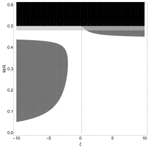
Figure 2: The black region is excluded because no static spherical shell can exist for $\mathsf{R}<\mathsf{R}_{2}\equiv M+\sqrt{M^{2}+Q^{2}}$ when $|Q|\leq M$. The translucent gray area contains static shell configurations with $Q/M=0$ which violate the dominant energy condition. The dark gray areas depict the regions where the “vacuum awakening effect” is triggered. The vertical dotted line corresponds to the conformal coupling, $\xi=1/6$. It intercepts the instability island inside the region where the dominant energy condition is violated. This graph should be used as a benchmark for the sake of comparison with Figs. 3, 4, and 5 where $Q/M\neq 0$.

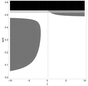
Figure 3: This figure considers a shell with $|Q|/M=0.5$. The same color convention as in Fig. 2 is assumed here.

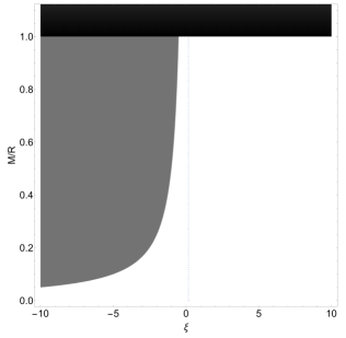
Figure 4: This figure considers a shell with $|Q|/M=1$. The same color convention as in Fig. 2 is assumed here. We see that the instability islands which appear in Figs. 2 and 3 for $\xi>0$ are not present in this case.

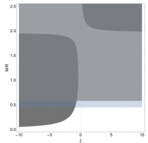
Figure 5: This figure considers a shell with $|Q|/M=1.5$. The dark region is not present here in contrast to the previous three figures because for $|Q|>M$ there are static shell configurations for any $M/\mathsf{R}$. On the other hand, the energy conditions are typically more restrictive. The light translucent gray area corresponds to configurations where the strong energy condition is violated. The dark translucent gray region is excluded by the weak, strong, and dominant energy conditions.

IV Vacuum energy density

Here, we analyze the exponential growth of the vacuum energy density (as measured by static observers) $\rho_{V}\equiv-\langle\hat{T}^{0}_{\;\;0}\rangle\equiv-\langle 0_{\rm in}|\hat{T}^{0}_{\;\;0}|0_{\rm in}\rangle$ as a result of the instability induced by the appearance of tachyonic modes. We assume the vacuum $|0_{\rm in}\rangle$ to be the no-particle state as defined according to the oscillating modes at the infinite past, where the initial shell parameters, $M_{\it in}$, $Q_{\it in}$, and $\mathsf{R}_{\it in}$, do not allow for the existence of tachyonic modes. Then, by assuming that the shell evolves to the static configuration, characterized by $M$, $Q$, and $\mathsf{R}$, which allows for the existence of tachyonic modes, we can use the general expression obtained in Ref. lv to write the leading contribution to the vacuum energy density (see Ref. llmv for a more comprehensive discussion):

$$\rho_{V}=-\langle\hat{T}^{0}_{\;\;0}\rangle^{-}H(-\ell)-\langle\hat{T}^{0}_{\;\;0}\rangle^{+}H(\ell)-\langle\hat{T}^{0}_{\;\;0}\rangle_{\cal S},$$ (55)

where $H(\ell)$ is the Heaviside step function (with $\ell$ being the proper distance of the geodesics which orthogonally intercept $\cal{S}$) and

$$\langle\hat{T}^{0}_{\;\;0}\rangle^{-}\sim-\frac{\kappa}{8\pi}\frac{e^{2\bar{\Omega}t}}{r^{2}}\frac{d}{dr}\left[\left(\frac{1-4\xi}{4\bar{\Omega}}\right)r^{2}\frac{d(\psi^{-}_{\bar{\Omega}0}(r)/r)^{2}}{dr}\right],$$ (56)

$$\langle\hat{T}^{0}_{\;\;0}\rangle^{+} \sim-\frac{\kappa}{8\pi}\frac{e^{2\bar{\Omega}t}}{r^{2}}\frac{d}{dr}\left[\left(\frac{1-4\xi}{4\bar{\Omega}}\right)r^{2}f(r)\frac{d(\psi^{+}_{\bar{\Omega}0}(r)/r)^{2}}{dr}\right.$$

$$\left.+\frac{\xi M}{{\bar{\Omega}}}\left(1-\frac{Q^{2}}{Mr}\right)\left(\frac{\psi^{+}_{\bar{\Omega}0}(r)}{r}\right)^{2}\right],$$ (57)

and

$$\langle\hat{T}^{0}_{\;\;0}\rangle_{\cal S} \sim-\frac{\kappa}{8\pi}e^{2\bar{\Omega}t}\frac{f(\mathsf{R})^{-1/2}}{\mathsf{R}}\frac{\xi}{\bar{\Omega}}\left[(1-4\xi)\left(-2+\frac{3M}{\mathsf{R}}\right.\right.$$

$$\left.\left.-\frac{Q^{2}}{\mathsf{R}^{2}}+2f(\mathsf{R})^{1/2}\right)+\frac{M}{\mathsf{R}}-\frac{Q^{2}}{\mathsf{R}^{2}}\right]\left(\frac{\psi^{+}_{\bar{\Omega}0}(\mathsf{R})}{\mathsf{R}}\right)^{2}\delta(\ell),$$ (58)

are the leading vacuum contributions to the energy density inside, outside, and on the shell, respectively. Here, $\kappa$ is a positive constant of order one (see Ref. lv for more details) and $\bar{\Omega}$ represents the largest $\Omega$ among all tachyonic solutions. We note that although the absolute value of the vacuum energy density increases exponentially in time, the growth is positive at some places and negative at some other ones in such a way that the total vacuum energy is conserved lv . Eventually, the spacetime must react to the vacuum energy growth leading the whole system to evolve into some final stable configuration with no tachyonic modes. The analysis of the corresponding evolution in the context of semiclassical gravity is well known to be difficult. However, it was recently shown that the scalar field should lose coherence fast enough to allow backreaction to be treated in the much easier context of general relativity llmv2 .

V Conclusions

We have analyzed the stability of a nonminimally coupled free scalar field in the spacetime of charged spherical shells. The impact of the charge on the instability is enhanced for more compact configurations. Also, the cases $|Q|\leq M$ and $|Q|>M$ differ because in the latter case there are static shell configurations for every radius $\mathsf{R}$. Notwithstanding, some of them may violate the weak, strong and dominant energy conditions. The presence of charge does not alter the fact that spherically symmetric shells which are able to awake the vacuum for conformally coupled scalar fields, $\xi=1/6$, do not satisfy at least the dominant energy condition. Finally, we have calculated the expectation value of the vacuum energy density in order to make explicit its exponential growth in time.

- (1) W. C. C. Lima and D. A. T. Vanzella, Gravity-induced vacuum dominance, Phys. Rev. Lett. 104, 161102 (2010).
- (2) R. F. P. Mendes, G. E. A. Matsas, and D. A. T. Vanzella, Quantum versus classical instability of scalar fields in curved backgrounds, Phys. Rev. D 89, 047503 (2014).
- (3) W. C. C. Lima, G. E. A. Matsas, and D. A. T. Vanzella, Awaking the vacuum in relativistic stars, Phys. Rev. Lett. 105, 151102 (2010).
- (4) A. G. S. Landulfo, W. C. C. Lima, G. E. A. Matsas, and D. A. T. Vanzella, Particle creation due to tachyonic instability in relativistic stars, Phys. Rev. D 86, 104025 (2012).
- (5) J. Novak, Neutron star transition to a strong-scalar-field state in tensor-scalar gravity, Phys. Rev. D 58, 064019 (1998).
- (6) P. Pani, V. Cardoso, E. Berti, J. Read, and M. Salgado, Vacuum revealed: The final state of vacuum instabilities in compact stars, Phys. Rev. D 83, 081501 (2011).
- (7) M. Ruiz, J. C. Degollado, M. Alcubierre, D. Núñez, and M. Salgado, Induced scalarization in boson stars and scalar gravitational radiation, Phys. Rev. D 86, 104044 (2012).
- (8) R. F. P. Mendes, Possibility of setting a new constraint to scalar-tensor theories, Phys. Rev. D 91, 064024 (2015).
- (9) C. Palenzuela and S. L. Liebling, Constraining scalar-tensor theories of gravity from the most massive neutron stars, arXiv:1510.03471.
- (10) W. C. C. Lima, R. F. P. Mendes, G. E. A. Matsas, and D. A. T. Vanzella, Awaking the vacuum with spheroidal shells, Phys. Rev. D 87, 104039 (2013).
- (11) R. F. P. Mendes, G. E. A. Matsas, and D. A. T. Vanzella, Instability of nonminimally coupled scalar fields in the spacetime of slowly rotating compact objects, Phys. Rev. D 90, 044053 (2014).
- (12) D. G. Boulware, Naked singularities, thin shells, and the Reissner-Nordström metric, Phys. Rev. D 8, 2363 (1973).
- (13) E. Poisson, A Relativist’s Toolkit (Cambridge University Press, Cambridge, England, 2004).
- (14) E. F. Eiroa and C. Simeone, Stability of charged thin shells, Phys. Rev. D 83, 104009 (2011).
- (15) S. A. Fulling, Aspects of Quantum Field Theory in Curved Space-time (Cambridge University Press, Cambridge, England, 1989).
- (16) R. M. Wald, Quantum Field Theory in Curved Spacetime and Black Hole Thermodynamics (University of Chicago, Chicago, 1994).
- (17) W. C. C. Lima, Quantization of unstable linear scalar fields in static spacetimes, Phys. Rev. D 88, 124005 (2013).
- (18) B. Schroer and J. A. Swieca, Indefinite metric and stationary external interactions of quantized fields, Phys. Rev. D 2, 2938 (1970).
- (19) J. Castiñeiras and G. E. A. Matsas, Low-energy sector quantization of a massless scalar field outside a Reissner-Nordström black hole and static sources, Phys. Rev. D 62, 064001 (2000).
- (20) I. S. Gradshteyn and I. M. Ryzhik Table of Integrals, Series and Products (Academic Press, New York, 1980).
- (21) A. G. S. Landulfo, W. C. C. Lima, G. E. A. Matsas, and D. A. T. Vanzella, From quantum to classical instability in relativistic stars, Phys. Rev. D 91, 024011 (2015).