Objective Eulerian Coherent Structures
Abstract
We define objective Eulerian Coherent Structures (OECSs) in two-dimensional, non-autonomous dynamical systems as instantaneously most influential material curves. Specifically, OECSs are stationary curves of the averaged instantaneous material stretching-rate or material shearing-rate functionals. From these objective (frame-invariant) variational principles, we obtain explicit differential equations for hyperbolic, elliptic and parabolic OECSs. As illustration, we compute OECSs in an unsteady ocean velocity data set. In comparison to structures suggested by other common Eulerian diagnostic tools, we find OECSs to be the correct short-term cores of observed trajectory deformation patterns.
1 Introduction
Coherent structures behind material pattern formation in unsteady flows have received considerable attention (see, e.g., [30, 4, 28], for reviews). Among other mathematical advances ([13, 1, 5, 26, 29]), variational techniques have been developed to identify Lagrangian Coherent Structures (LCSs), the most influential cores of material deformation, in experimental and numerical velocity data ([16, 12, 11, 18, 10]).
Specifically, initial positions of hyperbolic LCSs (generalized stable and unstable manifolds), elliptic LCSs (generalized KAM tori) and parabolic LCSs (generalized jet cores) are now readily computable as solutions of differential equations defined over the initial configuration of a system [17]. Later positions of these LCSs are then obtained by advecting their initial positions under the flow map. By the objectivity (frame-invariance) of their underlying variational principles, variational LCSs transform properly under coordinate changes of the form
| (1) |
where is an arbitrary proper orthogonal tensor family generating time-dependent rotations, and is an arbitrary vector family introducing time-dependent translations of the frame [32].
All LCSs, however, are intrinsically tied to a specific finite time interval over which they exert their influence on nearby trajectories. This influence is an integrated one, filtering out short-term anomalies in the flow. Yet short-term variability in material structures is often seen as significant in highly unsteady flows, explaining the popularity of Eulerian (i.e., instantaneous velocity-based) diagnostic fields in fluid dynamics (see, e.g., [21, 15], and [6] for reviews).
Eulerian diagnostics generally highlight features of the velocity field in a given frame of reference. Most studies of flows, nevertheless, would ideally want to understand, forecast or control the evolution and mixing of material trajectories, as well as the transport of the physical properties they carry. Indeed, the motivation for each commonly used Eulerian diagnostic is invariably grounded in the desire to understand particle motion over short time scales. Yet the approximations and heuristics employed in deriving these diagnostics, as well as the expectation for simply implementable results, tends to change the original focus of these approaches from material features to the analysis of frame-dependent velocity features.
Even short-term identifications of material coherence, however, must be frame-invariant by definition. This is because material coherent structures are composed of trajectories, which do not depend on coordinates and hence must transform properly under (1) from the frame of one observer to the other’s. If a proposed coherent structure criterion labels different material sets as coherent in different frames, then it either lacks a proper physical foundation, or its physical foundation is implemented through erroneous mathematics. Either way, the criterion cannot be used reliably in now-casting or real-time decision-making under unsteady flow conditions [29].
The few available objective Eulerian coherent structure diagnostics include that of Tabor and Klapper [31], who consider a point elliptic (i.e, part of a vortex) if the vorticity expressed in the basis of the rate-of-strain eigenvectors dominates strain (see also [24, 23]). Another objective Eulerian technique is the recent global approach [19] to rotationally coherent vortices. Identified as outermost closed level sets of the instantaneous vorticity deviation (IVD) from the spatial mean vorticity, IVD-based vortex boundaries are objective, short-term limits of closed curves obtained from a global Lagrangian rotational coherence principle.
Here we introduce a more general approach to Objective Eulerian Coherent Structures (OECSs) in two dimensions. We effectively seek these structures as short-term limits of LCSs. In contrast to [19], we use stretching-based variational LCS theories in taking this limit. As a consequence, we obtain a broader class of OECSs that includes elliptic (vortex-type), hyperbolic (stretching or contracting) and parabolic (jet-type) structures.
We give an explicit parametrization of all these types of OECSs as solutions of autonomous ordinary differential equations (ODEs). Our approach is global, eliminating the shortcomings of local structure identification schemes noted in [25]. All OECSs are computable without dependence on any chosen time scale. They are also objective, depending solely on invariants of the rate-of-strain tensor, i.e., the symmetric part of the velocity gradient.
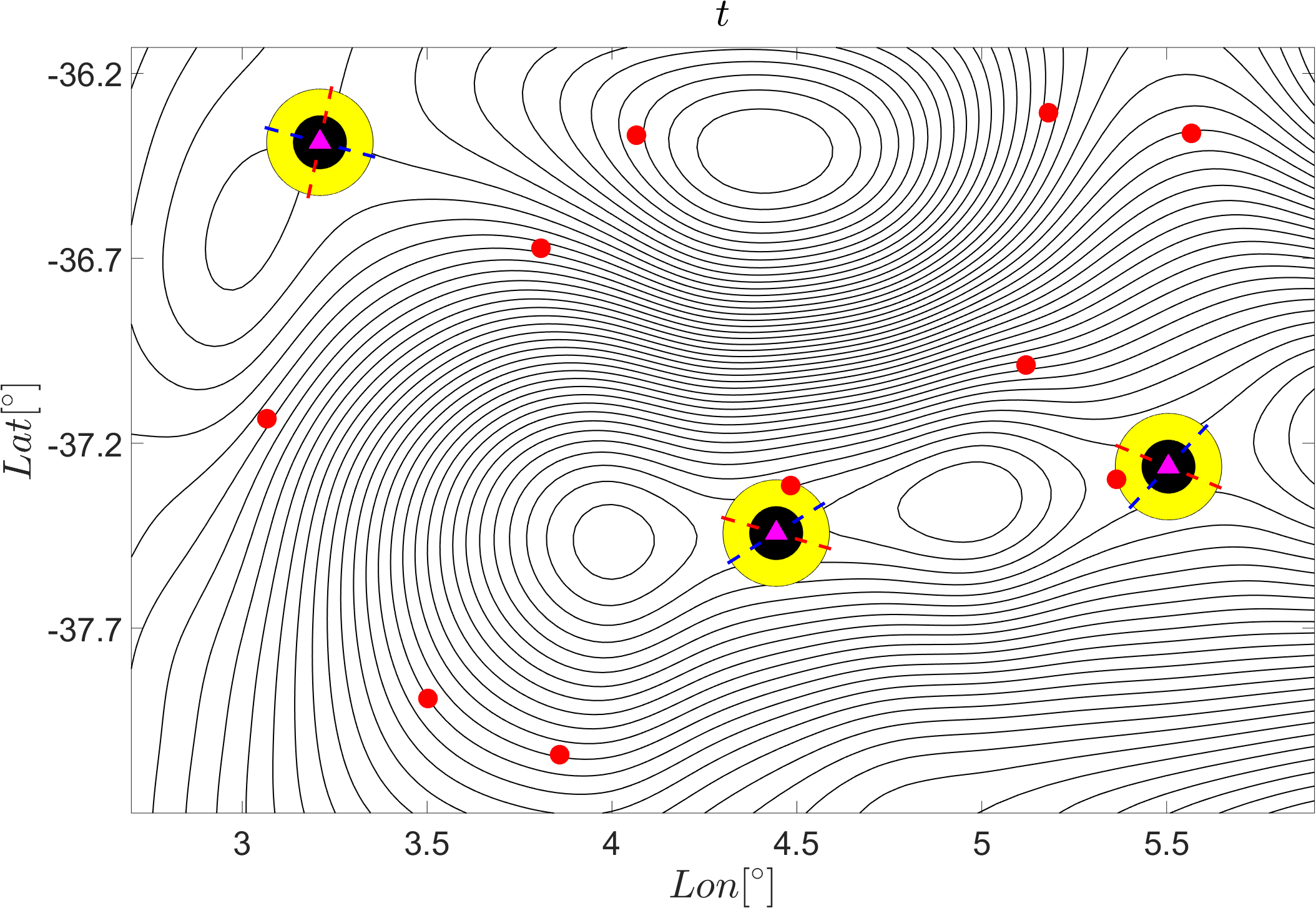
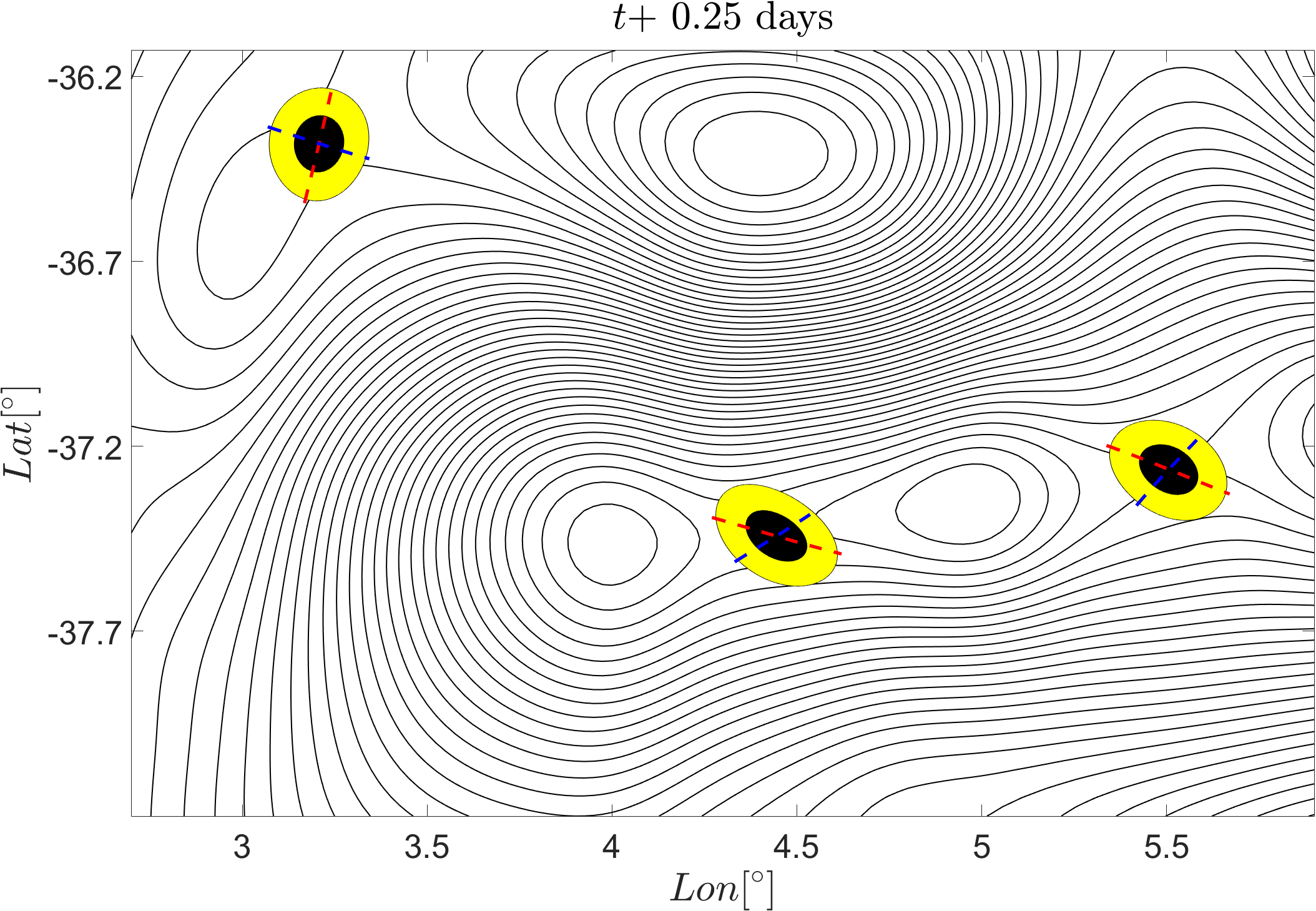
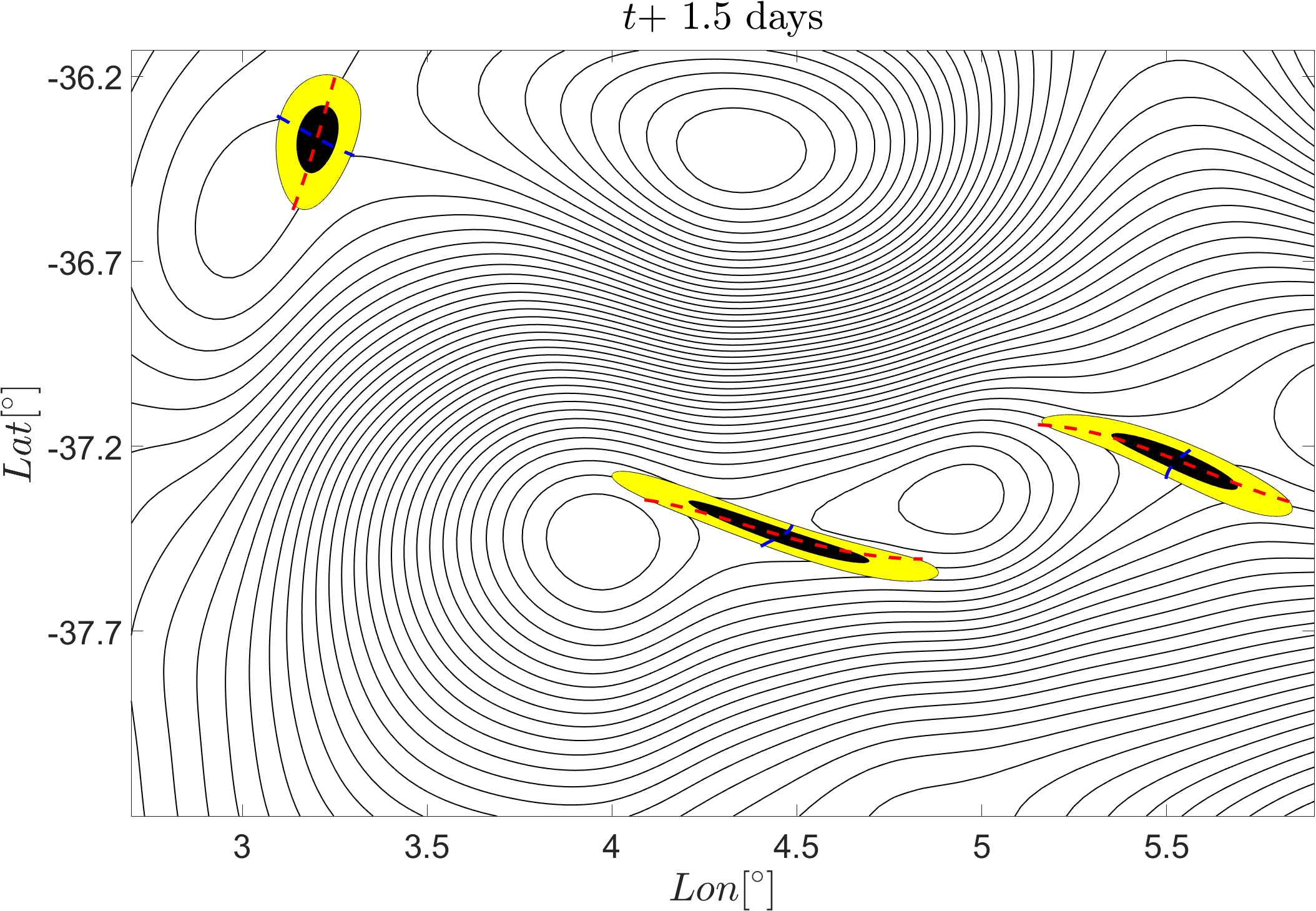
As an illustration of the results we derive here, Fig. 1 compares hyperbolic OECSs and the classic frame-dependent saddle-type stagnation points computed on an ocean velocity data (see section 8 for more detail). The effect of those structures on nearby particles and the instantaneous streamlines are also shown. In particular, Figs. 1a-1b show the attracting hyperbolic OECSs (red) with their cores (red dots) and the saddle-type stagnation points (magenta triangles) with their unstable directions (magenta) at the initial time, and after short-term advection. In contrast, Figs. 1c-1d show the same features observed from a frame translating in the longitudinal direction with constant speed (-0.6 degree/day), relative to the one used in Figs. 1a-1b.
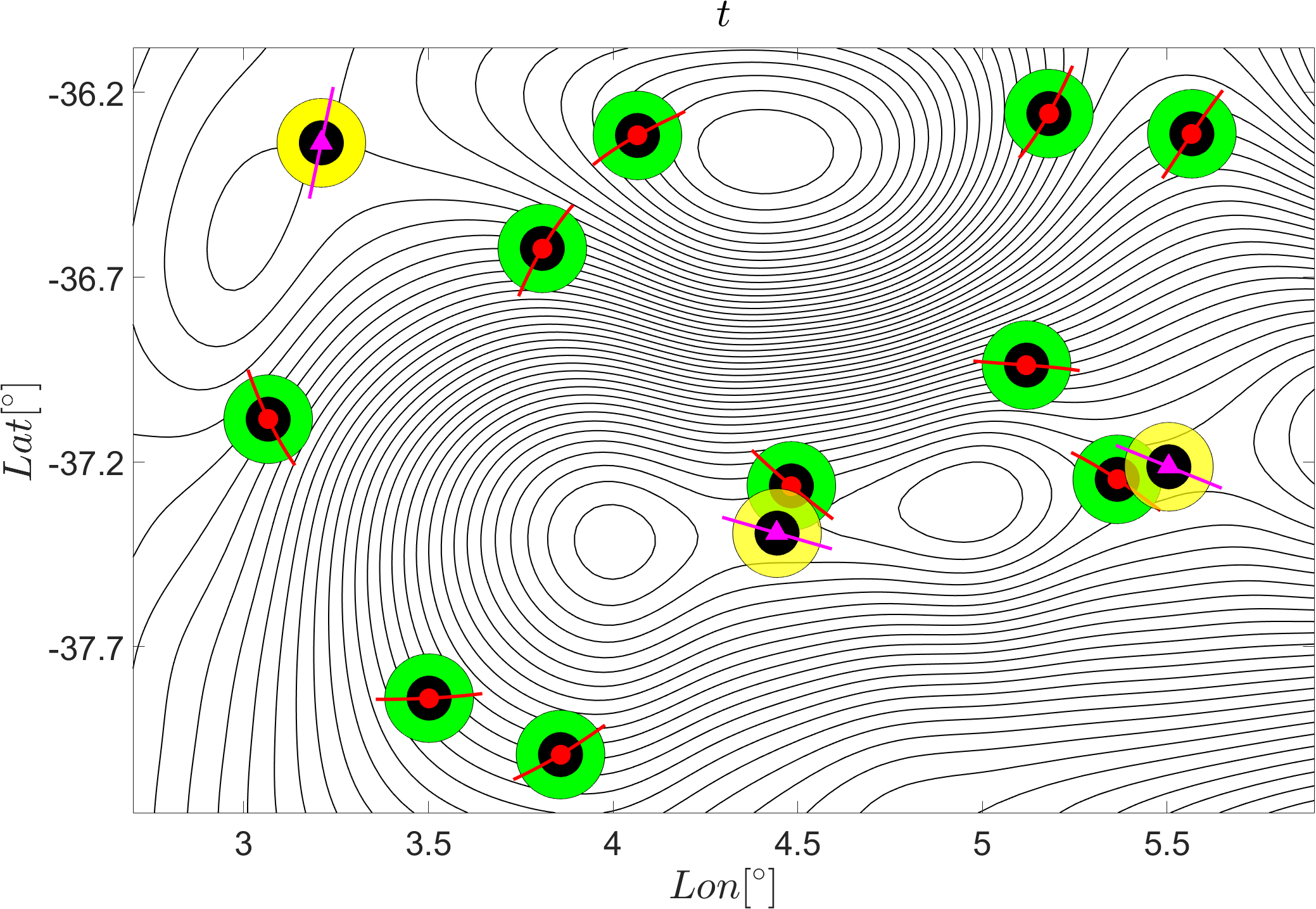
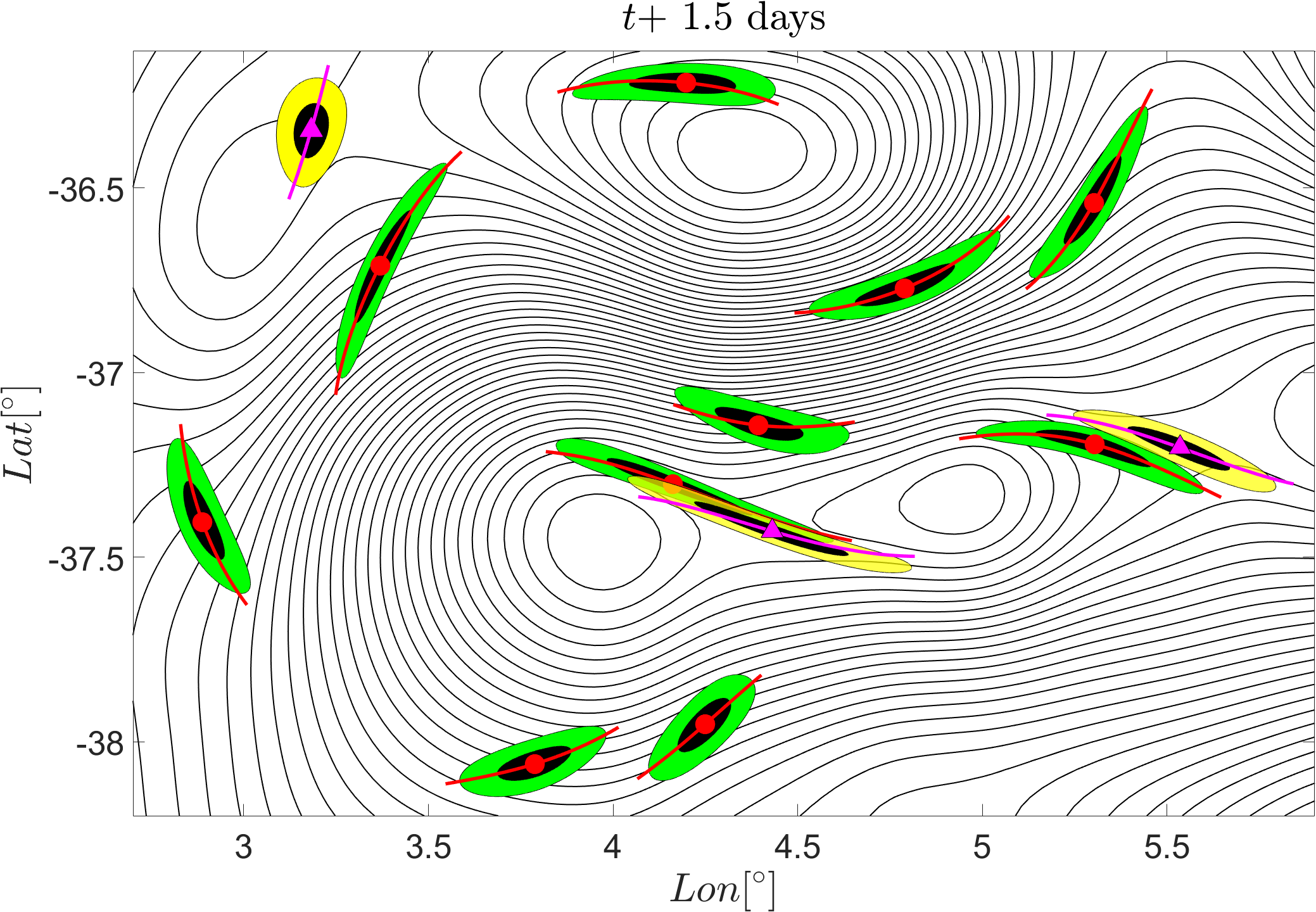

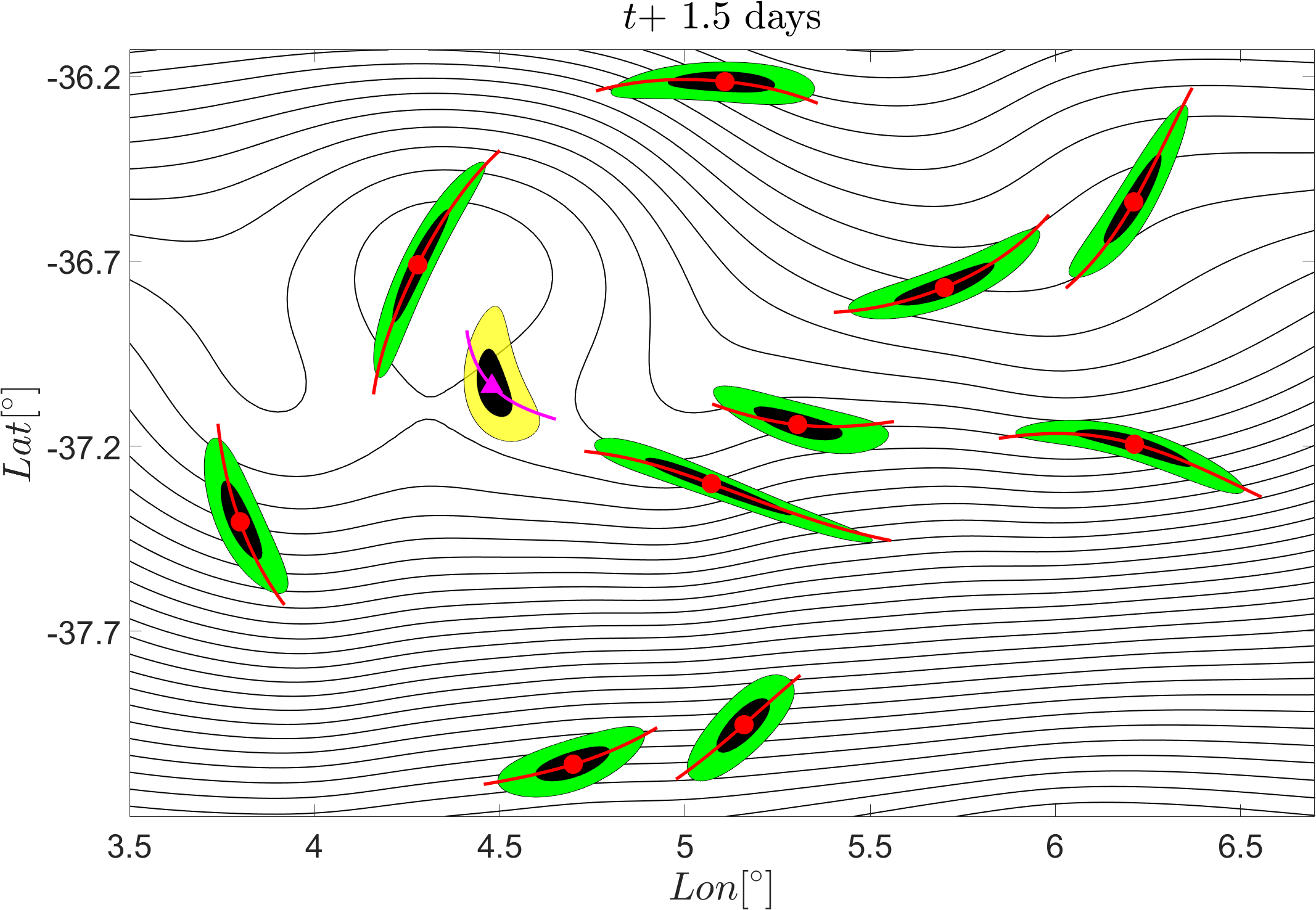
This example highlights two important facts. First, frame-dependent diagnostics, such as instantaneous stagnation points, are unsuitable for the self-consistent identification of coherent structures: the three saddle-type stagnation points detected by one observer (Figs. 1a-1b) disappear when the same phenomenon is analyzed by another observer in a moving frame (Figs. 1c-1d). In this second frame, a single saddle-type stagnation point emerges at an unrelated location and induces no notable material stretching.
Second, and more important, hyperbolic OECSs capture actual saddle-type material behavior in several locations with no stagnation points in their vicinities. Similar conclusions hold for elliptic and parabolic OECSs (cf. section 8). Based on this example, we expect OECSs to be useful in a number of physical situations where reliable now-casting, or short-term forecasting and control of material transport is critical.
We develop a theoretical foundation for our global variational OECS theory in sections 1-5. Readers interested mainly in a practical implementation of automated OECSs detection may proceed directly to section 6, which gives a summary of the results along with corresponding numerical schemes. In section 7, we perform OECSs detection in a two-dimensional ocean velocity data obtained from satellite altimetry. We show that variational OECSs outperform traditional Eulerian diagnostics in locating the skeletons of short-term material deformation.
2 Set-up and notation
Consider the two-dimensional non-autonomous dynamical system
| (2) |
with a twice continuously differentiable velocity field defined over an open flow domain , over a time interval We recall the customary velocity gradient decomposition
with the rate-of-strain tensor and the spin tensor . By our assumptions, and are continuously differentiable in and Under an observer change (1), the new rate-of-strain tensor and the new spin tensor are obtained in the form
| (3) | ||||
as shown is classic texts on continuum mechanics (see, e.g., [32]). Therefore, the rate-of-strain tensor is objective, as it transforms as a linear operator, whereas the spin tensor is not objective.
The eigenvalues and eigenvectors of are defined, indexed and oriented here through the relationship
| (4) |
We also recall that the rate of length change for an infinitesimal material element vector based at is
| (5) |
A further key relationship between the flow map of (2) and is obtained by considering the right Cauchy–Green strain tensor
| (6) |
whose temporal Taylor expansion around the initial time can be computed as
| (7) |
In other words, for small enough times, the leading order Lagrangian deformation is governed by the Eulerian rate-of-strain tensor. This observation enables us to consider Eulerian coherent structures as short-time limits of Lagrangian coherent structures.
3 Objective deformation rates
At an arbitrary time , consider a smooth curve , parametrized in the form by its arclength . Then the unit vectors and , with the rotation matrix appearing in (4), define a local tangent and a local normal to at the point . The following definition fixes the notions of instantaneous material shear rate and material stretching rate along While these quantities are intuitively clear, we also give their detailed derivation in Appendix A as first-order terms in the temporal Taylor expansion of the analogous finite-time Lagrangian shear and stretching measures (cf. [17]).
Definition 1.
Material deformation rates at time along a material curve with arclength parametrization :
-
1.
Material stretching rate:
-
2.
Material shear rate:
(8)
Physically, gives the instantaneous tangential stretching rate along , while represents twice the rotation rate due to shear of an initially normal perturbation to . The objectivity of these Eulerian deformation rate measures follows from (3) together with the commutation between an arbitrary planar rotation and the ninety-degree rotation .
4 Variational principles for OECSs
Using the Eulerian deformation rates introduced in Definition 1, we now define the averaged stretch- and shear-rate functionals over an arbitrary curve at time :
Definition 2.
At time along the material curve :
-
1.
The averaged material stretch-rate is
(9) -
2.
The averaged material shear-rate is
(10)
By smooth dependence of on and , one expects to see variability in the average material stretch- or shear-rates across an strip of material lines surrounding Exceptional choices of , however, defy this trend, displaying only an variability of or in strips around Such curves will act as centerpieces of coherence in the material stretch-rate or material shear-rate fields.
This lack of leading order variability in the averaged stretch-rate or shear-rate along is equivalent to the vanishing of the first variation of the functional or on . The former case occurs on instantaneous vortex boundaries with no short-term unevenness in their tangential deformation (no short-term filamentation). The latter case arises for curves that are cores of short-term shear-type deformation (instantaneous jets) or short-term hyperbolic stretching (instantaneous hyperbolic structures). We formalize these definitions below, using the time derivatives of the corresponding global variational LCS definitions reviewed in [17].
Definition 3.
At time
-
1.
A closed curve is an elliptic OECS if it is a stationary curve of the averaged stretch-rate functional , i.e.,
(11) -
2.
A curve is a shearless OECS if it is a stationary curve of the averaged shear-rate functional , i.e.,
(12)
The variational problems outlined in (11) and (12) are equivalent to the weak Euler-Lagrange equations
| (13) |
| (14) |
with denoting small perturbations to the curve . We discuss below the solutions of equations (13-14), building on similar ideas developed for LCSs ([18, 10]). This approach will lead to explicit solutions of(11)-(12), and enable a further partitioning of shearless OECSs into hyperbolic and parabolic OECSs.
5 Elliptic OECS
By Definition 3, an elliptic OECS is a closed curve, and hence its small perturbation used in calculating the first variation of along is also periodic with the same period . As a consequence, the first bracketed term in (13) vanishes. Then, by the fundamental lemma of the calculus of variations, equation (11) becomes equivalent to the classic Euler–Lagrange equations
| (15) |
The detailed form of this equation is similar to the Euler–Lagrange equation derived by [18] for elliptic LCSs (stationary curves of the averaged, finite-time tangential stretch along the material curve ). The only difference in the present context is that the expression for has no square root, and contains the rate-of-strain tensor instead of the Cauchy–Green strain tensor defined in (6). Therefore, following the procedure similar to the one adopted in [18], we obtain the following full characterization of elliptic OECSs.
Theorem 1.
Elliptic OECSs at time coincide with limit cycles of the differential equation family
| (16) |
defined for any parameter value on the set
Along any elliptic OECS obtained for a given value of , the material stretching rate at time is pointwise constant and equal to
The right-hand side of the differential equation (16) is only locally a vector field in , because the rate-of-strain eigenvector fields are generally not globally orientable in . Local orientability of in , however, is always possible. This makes the trajectories, and specifically the limit cycles, of the differential equation (16) well defined.
Along limit cycles obtained for , we have Such elliptic OECSs, therefore, are perfectly coherent in the Eulerian sense, exhibiting uniformly zero pointwise material stretching rate. The direction field ceases to be well-defined at locations of repeated rate-of-strain eigenvalues (). Following the terminology used in [18], we refer to such locations as singularities of the tensor field An appropriate extension of Poincaré’s classic index theory implies that there are at least two singularities of in the interior of any limit cycle of . This in turn leads to an automated detection algorithm that applies equally to elliptic OECSs. We refer to [22] for a detailed discussion of this algorithm for elliptic LCSs.
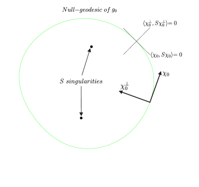
By their hyperbolicity (i.e., strict attraction or repulsion of nearby trajectories of the vector field ), elliptic OECSs are robust with respect to moderate errors and uncertainties in the underlying velocity field . Figure 2a summarizes the main properties of perfectly coherent elliptic OECSs. Detailed discussions on the numerical detection of limit cycles of directions fields can be found in [18] and [22] for LCS. These can be directly applied here after replacing with .
Under changes in the parameter , limit cycles of arise in continuous, non-intersecting families (see Appendix B). An Eulerian vortex boundary can then be defined as the outermost member of such an elliptic OECS family. Given the objectivity of each member of such a limit cycle family, Eulerian vortex boundaries defined in this fashion are also objective.
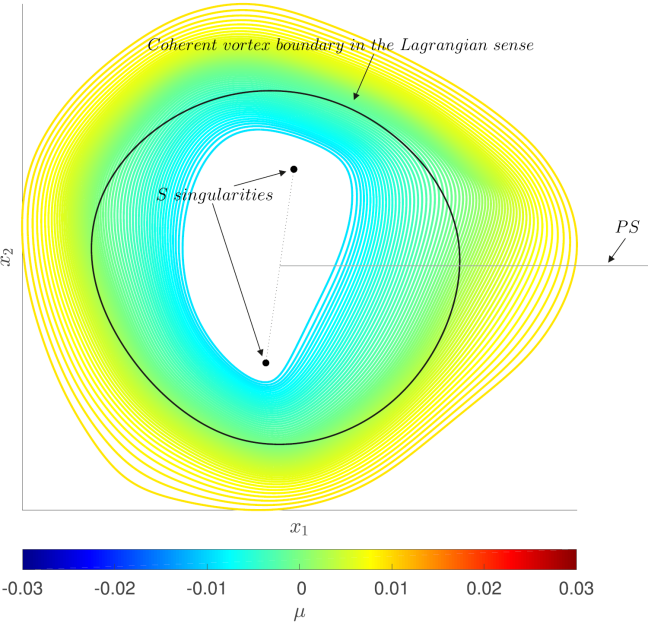
Figure 2b shows such a family and its outermost member in a flow example analyzed in more detail in section 10. A nested OECSs family often signals a nearby coherent Lagrangian vortex boundary, as is the case in Fig. 2b. Just as in the case of elliptic LCSs [18], solutions of the variational principle (11) can also be viewed as closed null-geodesics of a Lorentzian metric family
| (17) |
which has metric signature (-,+) [2]. The tensor family denotes a generalized rate-of-strain tensor and the parameter denotes the instantaneous tangential stretching rate on . In this context, locations of repeated eigenvalues of are singularities for the metric which becomes degenerate at these points (cf. Fig. 2).
6 Shearless OECS
By Definition 3, a shearless OECS at time is a stationary curve of the averaged shear-rate functional , and hence satisfies the weak Euler–Lagrange equation (14). We can pass to the strong form of these Euler–Lagrange equation if the first bracketed term in (14) vanishes for the class of admissible perturbations applied to the parametrization of the stationary curve we seek.
Following the procedure developed in [10] for elliptic LCS, we find the following class of admissible perturbations for which the boundary term in (14) vanishes:
- (BC1)
-
Variable-endpoint boundary conditions: The endpoints of coincide with singularities of the rate-of-strain tensor field , i.e., we have and . In this case, the perturbations are arbitrary, including arbitrary perturbations to the endpoints of .
- (BC2)
-
Fixed-endpoint boundary conditions: The perturbation is arbitrary for all but must leave the endpoints of fixed: .
Under (BC1) or (BC2), the bracketed term in (14) vanishes. By the fundamental lemma of the calculus of variations, a solution curve of (14) must then satisfy the Euler–Lagrange equations
| (18) |
Invoking the results of [10] for shearless LCSs, we obtain that solution curves of (18) with exactly vanishing shear rates are piecewise tangent to one of the eigenvector fields of .
Theorem 2.
Shearless OECSs at time coincide with continuous trajectories of the differential equation family
| (19) |
Along any such shearless OECS, the pointwise material shear rate at time is zero.
We refer to the trajectories of (19) as -lines and -lines, respectively. We will use the boundary condition classes (BC1)-(BC2) to further distinguish parabolic and hyperbolic OECSs within the shearless OECSs satisfying (19).
From an argument closely following [10], we obtain that the solutions of (18) can also be viewed as null-geodesics of the Lorentzian metric family
which again has metric signature (-,+) [2], and admits singularities at locations of repeated eigenvalues of . In particular, shearless OECSs are null geodesics of for
6.1 Parabolic OECS
Parabolic OECSs are trajectories of (19) that satisfy the free-endpoint boundary conditions (BC1) and are as close as possible to being neutrally stable, as detailed below. By the nature of (BC1), such OECSs are stationary curves of the shear-rate functional under the broadest possible set of perturbations. This makes parabolic OECSs the most observable class of shearless OECSs, creating short-term pathways that mimic the role of the Lagrangian jet cores identified in [10].
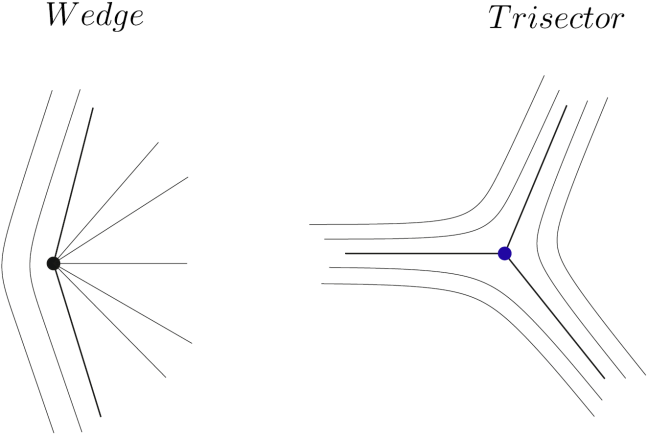
More specifically, parabolic OECSs are heteroclinic chains of lines and -lines connecting singularities of . For observability and uniqueness, we only consider alternating chains of - and -line connections that are locally unique and structurally stable. As shown in [8], the only structurally stable tensorline singularities are trisectors and wedges, shown in Fig. 3.
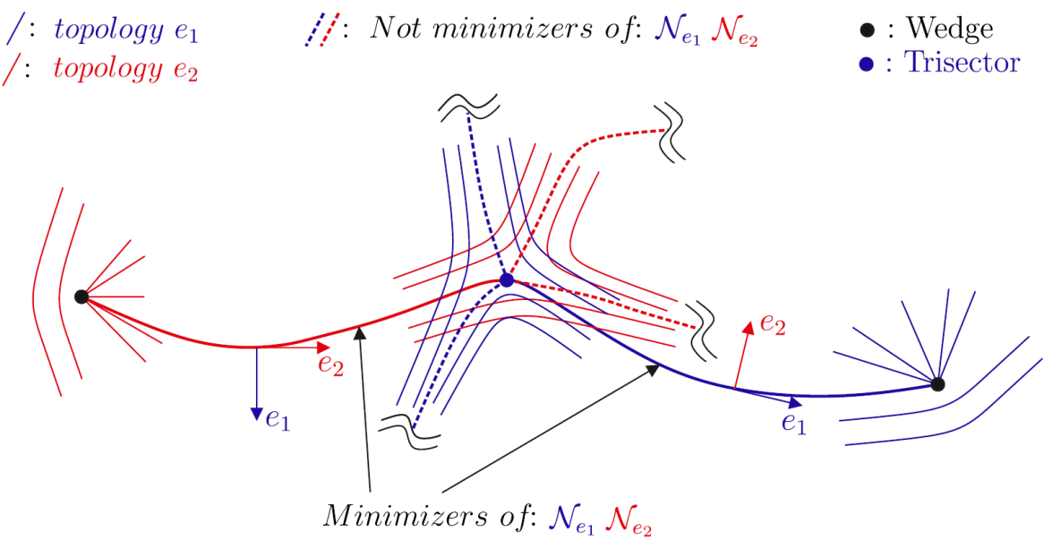
Furthermore, as shown in [10], a structurally stable and unique connection between two such singularities must necessarily be a wedge-trisector connection, as illustrated in Fig. 4.
By definition, each segment of an alternating chain of - and -lines repels or attracts trajectories over short enough time intervals. To ensure that neither attraction nor repulsion prevails for the whole trajectory chain, we require the chain to be as close as possible to being neutrally stable. To this end, we introduce the pointwise neutrality functions
| (20) |
with the function measuring how close the squared rate of attraction or repulsion, along an line is to zero at time . In case of incompressible flows, we have , given that .
All this follows closely the variational approach developed in [10] for parabolic LCSs, but with substituted for . As a next step, we introduce the convexity sets
| (21) |
Each such set is simply the set of points at which the corresponding neutrality is a convex function of at time . We say that a compact -line segment is a weak minimizer of at time if both and the nearest trench of the function lie in the same connected component of . More precisely, if the arclength parametrization of is , and the unit normal along is given by , then we require
| (22) |
where
| (23) |
We summarize our formal definition of parabolic OECSs as follows (cf. Fig. 4).
Definition 4.
A parabolic OECS at time is a shearless OECS composed of alternating chains of - and -line segments that connect wedge and trisector singularities of the the rate-of-strain tensor Furthermore, each segment in the chain is a weak minimizer of the neutrality function
6.2 Hyperbolic OECSs
Hyperbolic OECSs are trajectory segments of (19) that satisfy the fixed-endpoint boundary conditions (BC2) and contain precisely one point of maximal repulsion-rate or maximal attraction-rate. This point will then play the role of an instantaneous saddle point, with the OECSs acting as the short-term stable or unstable manifold for this saddle point. By the nature of (BC2), hyperbolic OECSs are only stationary curves of the shear-rate functional under variations that leave their endpoints fixed. This makes individual hyperbolic OECSs less observable than parabolic OECSs. This is also the case for hyperbolic LCSs, which are generally responsible for the intricate filamentation of tracer patterns. Details of these filaments are generally less observable and robust as those of Lagrangian jet cores marked by parabolic LCSs (cf. [10]).
Within the family of hyperbolic OECSs, we distinguish attracting OECSs as material curves that attract nearby material curves instantaneously. Similarly, we distinguish repelling OECSs as hyperbolic OECSs that instantaneously repel all nearby material curves. We summarize these definitions more formally as follows (cf. Fig. 5).
Definition 5.
A repelling OECS at time is an open -line segment that contains a local maximum of the function , but contains no other local extremum point of . An attracting OECS at time is an open -line segment that contains a local minimum of the function , but contains no other local extremum of . Finally, a hyperbolic OECS is a shearless OECS that is either an attracting or a repelling OECS.
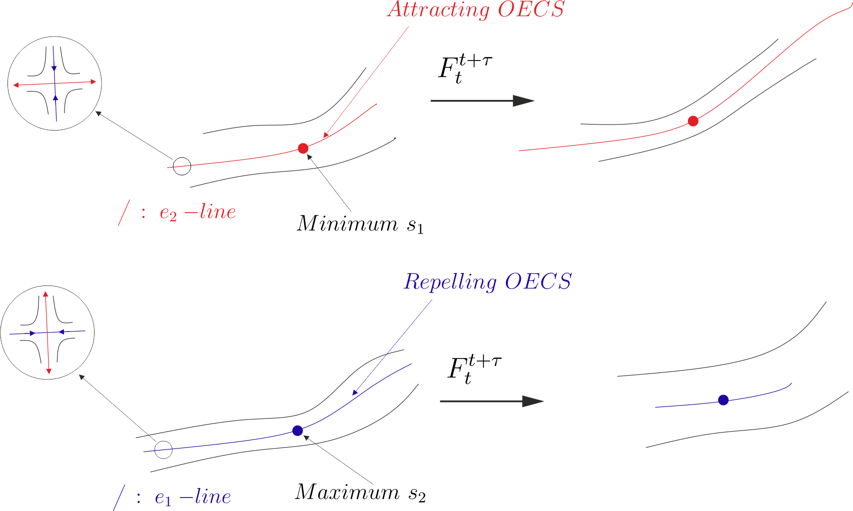
Remark 1.
As indicated in Fig. 5, the cores of hyperbolic OECSs are defined by a local maximum of along repelling OECSs and by a local minimum of along attracting OECSs. We call these cores objective saddle points, as they represent generalizations of classic saddle-type stagnation points from steady flows. Instantaneous stagnation points of an unsteady velocity field are not Galilean invariant, i.e., may disappear even under constant-speed translations of the coordinate frame (cf. Fig. 1). In contrast, the objective saddle points introduced here are objective, and hence persist even under general observer changes of the form (1). The local value of on the objective saddle quantifies the strength of that saddle objectively.
7 Summary of OECSs and their numerical identification
In Table 1, we list the OECSs we introduced in the previous section, together with the ODEs and boundary conditions they satisfy.
| s | ||
| Attracting | arbitrary; contains a local minimum of | |
| Repelling | arbitrary; contains a local maximum of | |
| Parabolic | with alternating | |
| Elliptic | Periodic |
Next, we summarize the numerical steps in locating OECSs in a planar unsteady flow. We start with the common steps, then detail the further steps for different types of OECSs separately.
Input: A 2-dimensional velocity field
-
1.
Compute the rate-of-strain tensor at the current time on a rectangular grid over the ) coordinates.
-
2.
Detect the singularities of as common, transverse zeros of and , with denoting the entry of at row and column .
-
3.
Determine the type of the singularity (trisector or wedge) as described in [10].
-
4.
Compute the eigenvalue fields and the associated unit eigenvector fields of for
Output: as well as and , for , and the position and type (wedge or trisector) of the rate-of-strain singularities satisfying
7.1 Elliptic OECSs
To locate elliptic OECSs automatically as limit cycles of the direction field (16), we rely on a version of Poincaré’s index theory extended to direction fields [7, 22]. A consequence of this theory is that at least two wedge-type singularities of must exist inside any such limit cycle [22]. For robust limit cycles, we seek nearby wedge pairs surrounded by an annular region of no singularities. The same procedure arises in elliptic LCS detection, involving the location of singularities of the tensor field We refer to [22] for details of this numerical algorithm.
Input: as well as and , for , and the position and type (wedge or trisector) of the rate-of-strain singularities satisfying
-
1.
Locate isolated wedge-type pairs of singularities and place the Poincaré sections at their midpoint.
-
2.
Compute the vector field defined in (16) for different values of stretching rate , remaining in the range .
-
3.
Use the Poincaré sections as sets of initial conditions in the computation of limit cycles of
where the factor multiplying removes potential orientational discontinuities in the direction field away from singularities, and denotes the integration step in the independent variable .
Output: Elliptic OECSs.
7.2 Hyperbolic OECSs
Input: as well as and , for .
-
1.
Compute the sets of isolated local maxima of for .
-
2.
Compute attracting OECSs (–lines) as solutions of the ODE
Stop integration when ceases to be monotone decreasing.
-
3.
Compute repelling OECSs (–lines) as solutions of the ODE
Stop integration when ceases to be monotone decreasing.
Output: Hyperbolic OECSs.
7.3 Parabolic OECSs
Input: as well as and , for , and the position and type (wedge or trisector) of the rate-of-strain singularities satisfying
-
1.
For each trisector-type singularity , compute the -lines and -lines connecting the trisector to a wedge.
- 2.
-
3.
With the separatrices obtained in this fashion, build alternating chains of heteroclinc -lines and -lines
Output: Parabolic OECSs.
8 Example: Mesoscale OECSs in large-scale ocean data
We use Algorithms 1-4 from section 6 to locate OECSs in a two-dimensional ocean surface velocity data set derived from AVISO satellite altimetry measurements (http://www.aviso.oceanobs.com). The domain of interest is the Agulhas leakage in the Southern Ocean bounded by longitudes , latitudes and the time slice we selected correspond to .
Under the geostrophic assumptions, the ocean surface height measured by satellites plays the role of a streamfunction for surface currents. With denoting the sea surface height, the velocity field in longitude latitude coordinates, , can be expressed as
where denotes the Coriolis parameter, the constant of gravity, the mean radius of the hearth and its mean angular velocity. The velocity field is available at weekly intervals, with a spatial longitude-latitude resolution of . For more detail on the data, see [3].
8.1 Elliptic OECSs
Following Algorithm 1 in section 6.1, we locate singularities of the rate-of-strain tensor , and discard isolated wedge singularities whose distance to the closest wedge point is larger than the typical mesoscale distance of . The remaining wedge pairs mark candidate regions for elliptic OECSs.
Along with elliptic OECSs, we will also show the value of the Okubo–Weiss (OW) parameter
where denotes the vorticity. Spatial domains with are frequently used indicator of instantaneous ellipticity in unsteady fluid flows [27, 33]. While the OW parameter is not objective (the vorticity term will change under rotations), its simplicity makes it broadly used in locating coherent vortices.
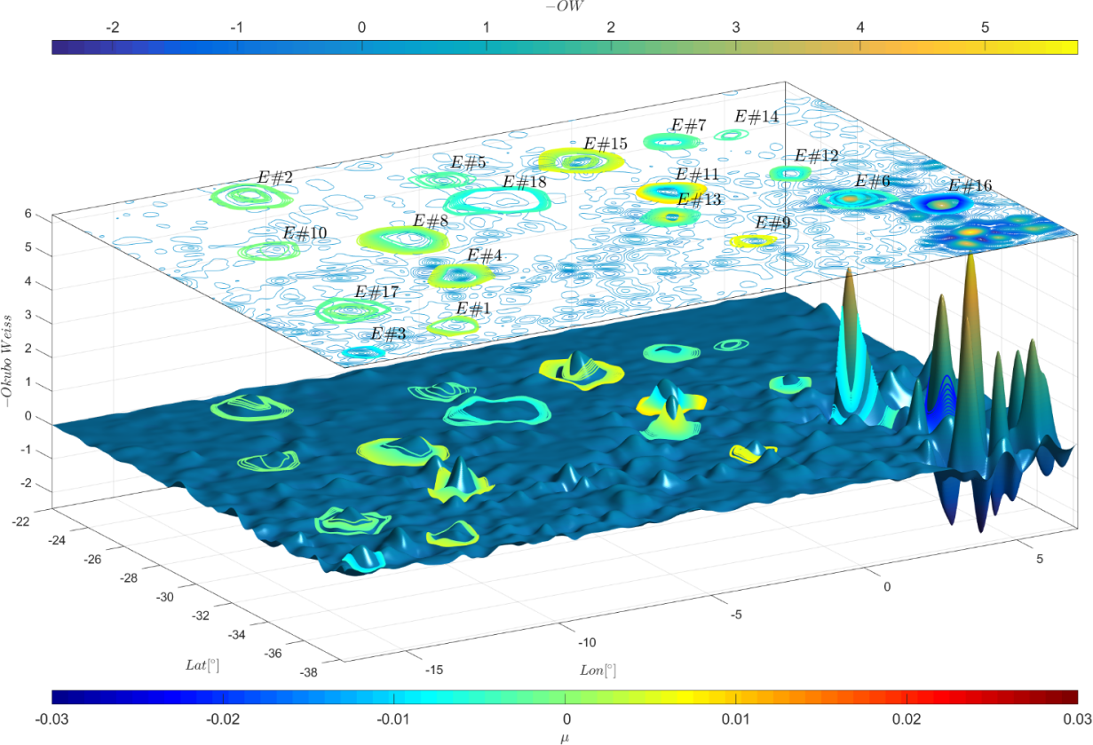
In the domain of study, we obtain a total of eighteen objectively detected vortical regions, each filled with families of elliptic OECSs. We plot these families over a two-dimensional graph of , and also project them onto the level curves of in the plane (Fig. 6).
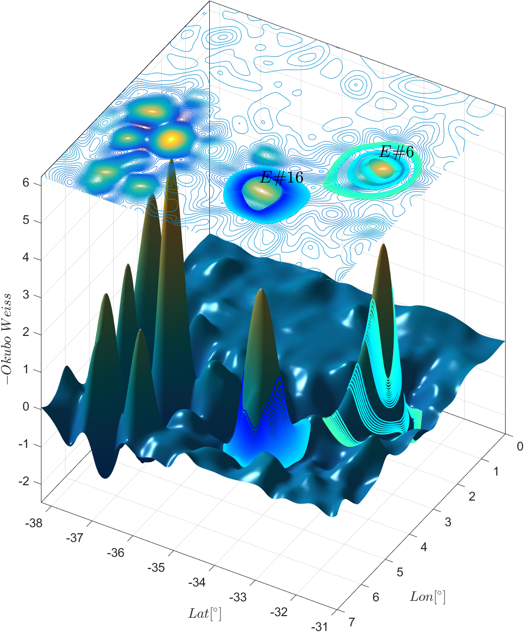
Note that the objective vortical regions and arise in regions where is nearly zero and hence indicates no significant vortical activity. At the same time, at the bottom right region of the domain, attains several strong local minima, even though there are no elliptic OECSs present (cf. Fig. 6b).
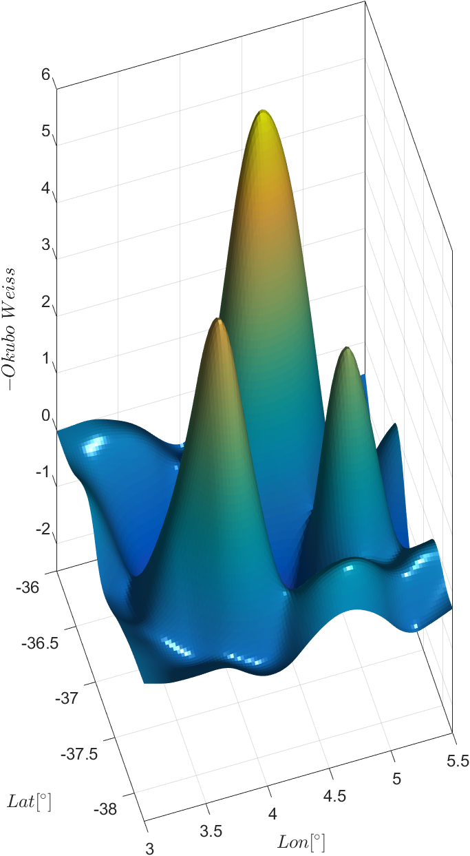
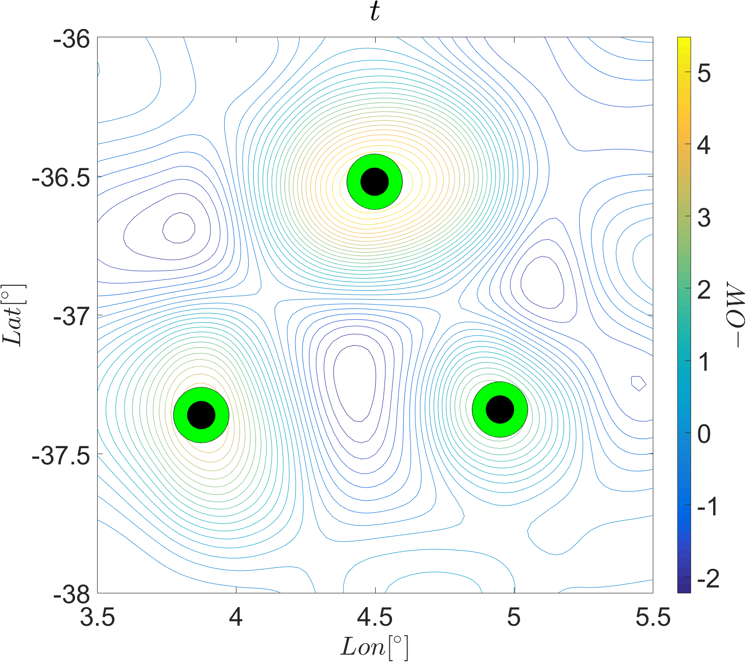
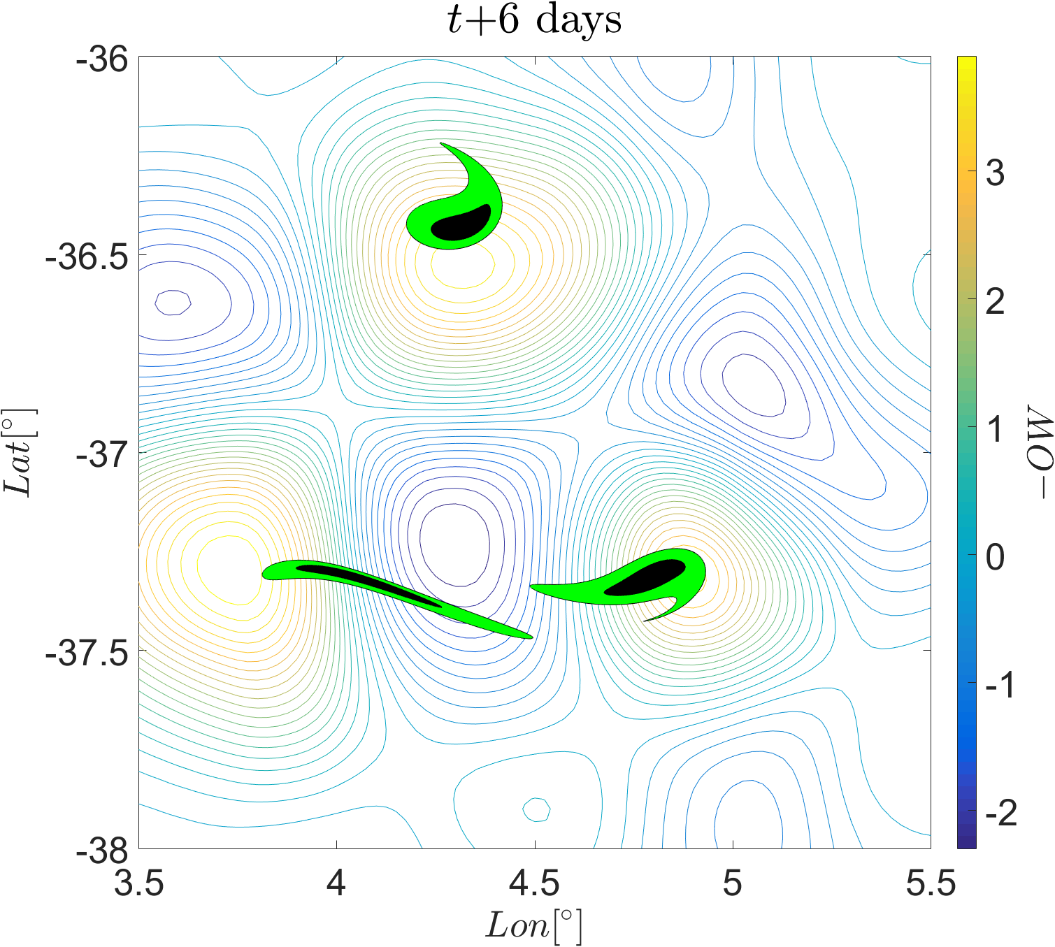
As a representative example, we show in Fig. 7 the three strongest local minima of in this region along with the deformation of material blobs, initially centered on those minima, for an integration time of six days. For comparison, Fig. 8 shows the deformation experienced by blobs initialized within two elliptic OECSs for different integration times, up to six days.
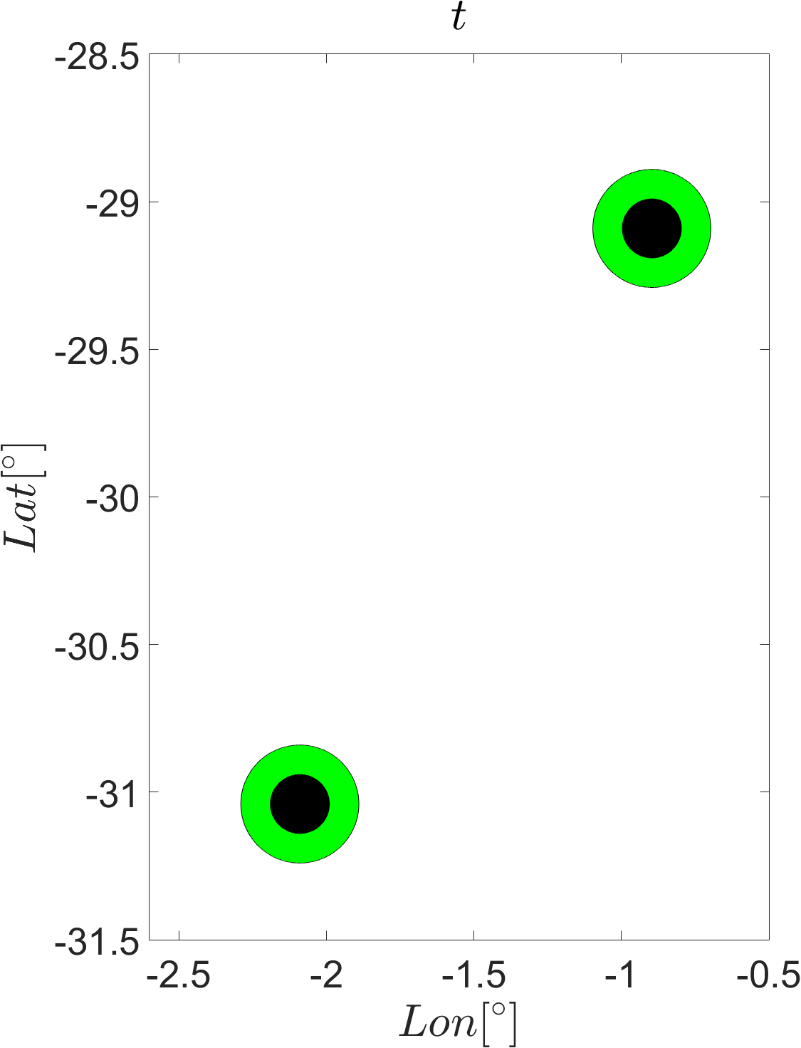
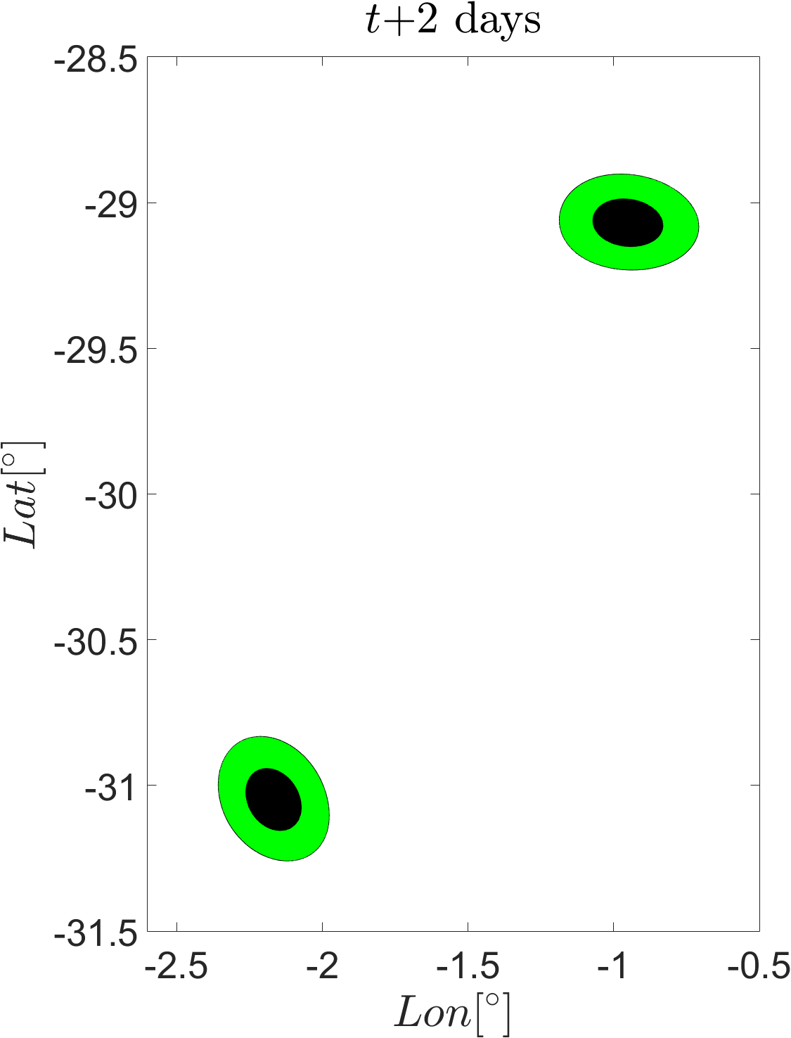
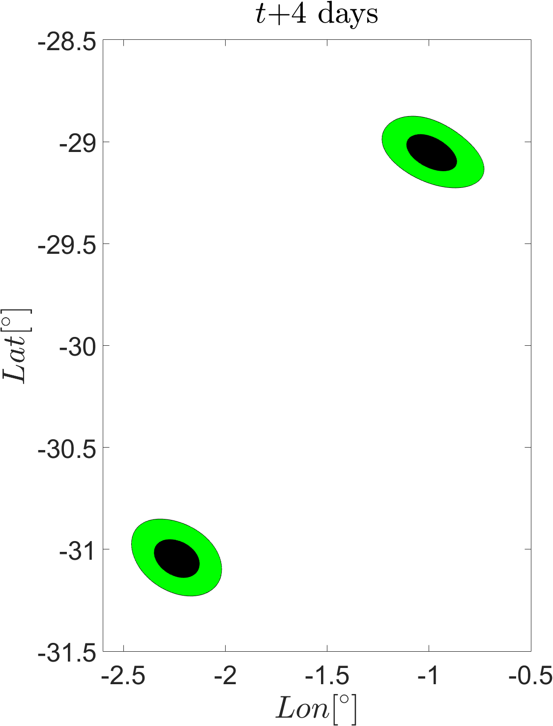
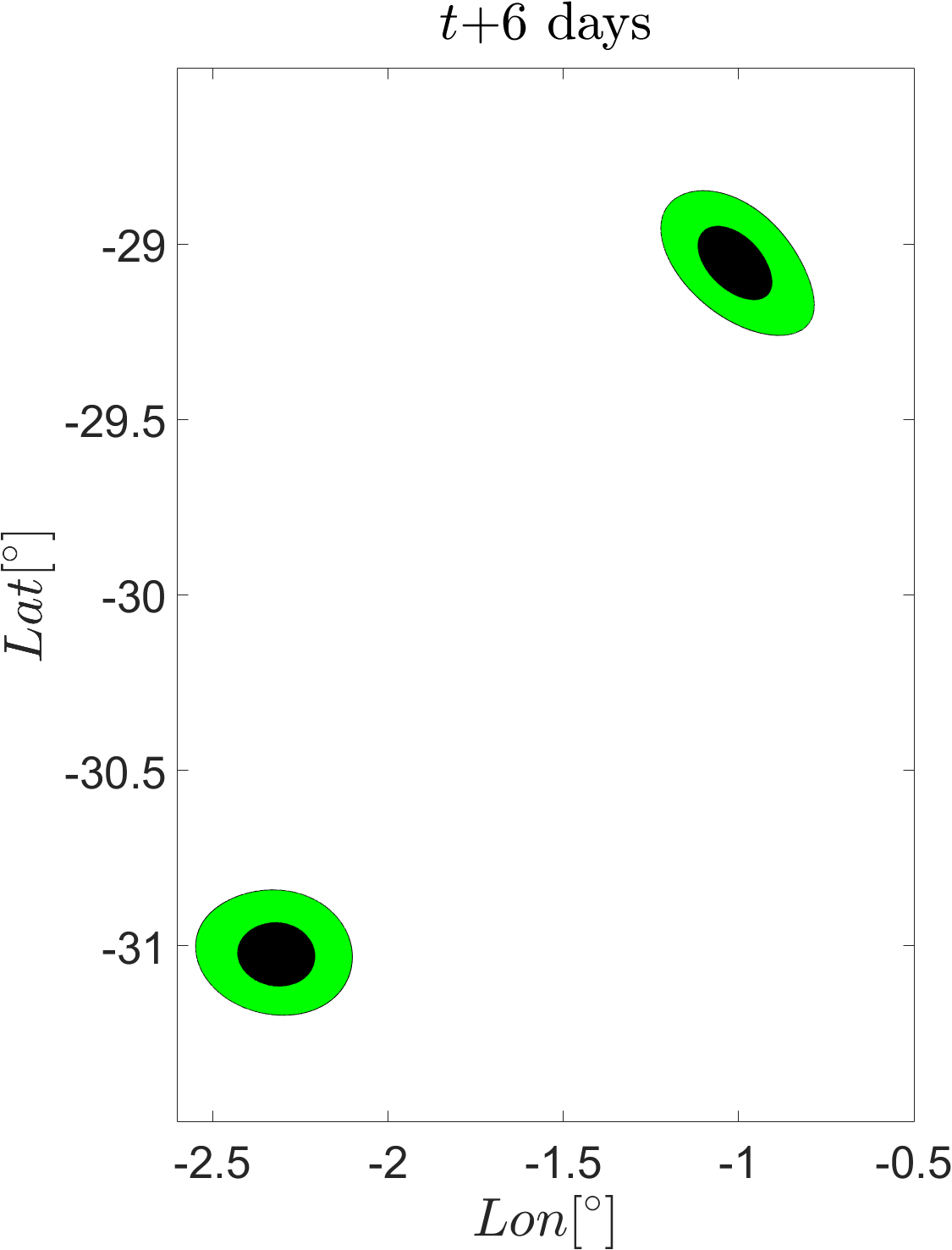
The blobs in Fig. 8 barely deform, and hence instantaneously computed elliptic OECSs exhibit short-term Lagrangian vortex-type behavior, as expected.
Hence, the regions of highest ellipticity for the Okubo-Weiss parameter show significant stretching, while regions identified by elliptic OECSs remain highly coherent over the same time interval. We have, therefore, clear examples of both false positives and false negatives for Okubo–Weiss-based vortex detection.
The vortical regions approximate locations where exceptionally coherent Lagrangian coherent eddies have been found in other studies (see [22], [18]). These Lagrangian studies cover a time interval of three months, with their initial time coinciding with the time of the present Eulerian analysis. Remarkably, about one third of the elliptic OECSs we find are signatures of elliptic LCSs with long-term coherence.
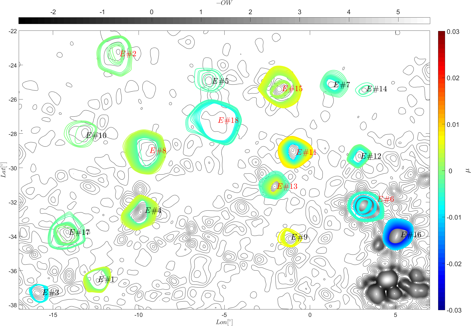
Figure 9 underlines this observation by showing the top view of Fig. 6a separately, using a different colormap for the scalar field, and tagging with red numbers elliptic OECSs in the coherent Lagrangian eddy domains identified by [18]. Without exception, these regions are marked by near-zero values of the stretching rate, indicating a high degree of Eulerian coherence for the elliptic OECSs.
In contrast, most of these highly coherent Lagrangian eddies have very moderate signatures in the contour plot of the Okubo–Weiss parameter. Taking all regions of closed level sets with comparable values as predictions for coherent eddies would results in an order-of-magnitude over-prediction for vortical regions. This is consistent with the findings of [3], which reports a roughly tenfold over-prediction of the actual number of coherent Agulhas eddies by the Okubo–Weiss criterion.
8.2 Hyperbolic OECSs
We compute hyperbolic OECSs at the same time used in our elliptic
OECSs calculations, on a subdomain bounded by longitudes
and latitudes . Since the velocity
field is incompressible, the maxima of coincide with the
minima of . Consequently, the same OECS cores arise as starting
points in the computation of both attracting and repelling hyperbolic
OECSs. We show all hyperbolic OECSs so obtained in Fig. 10.
As noted earlier, the cores of hyperbolic OECSs represent the objective
saddle points in the unsteady velocity field.
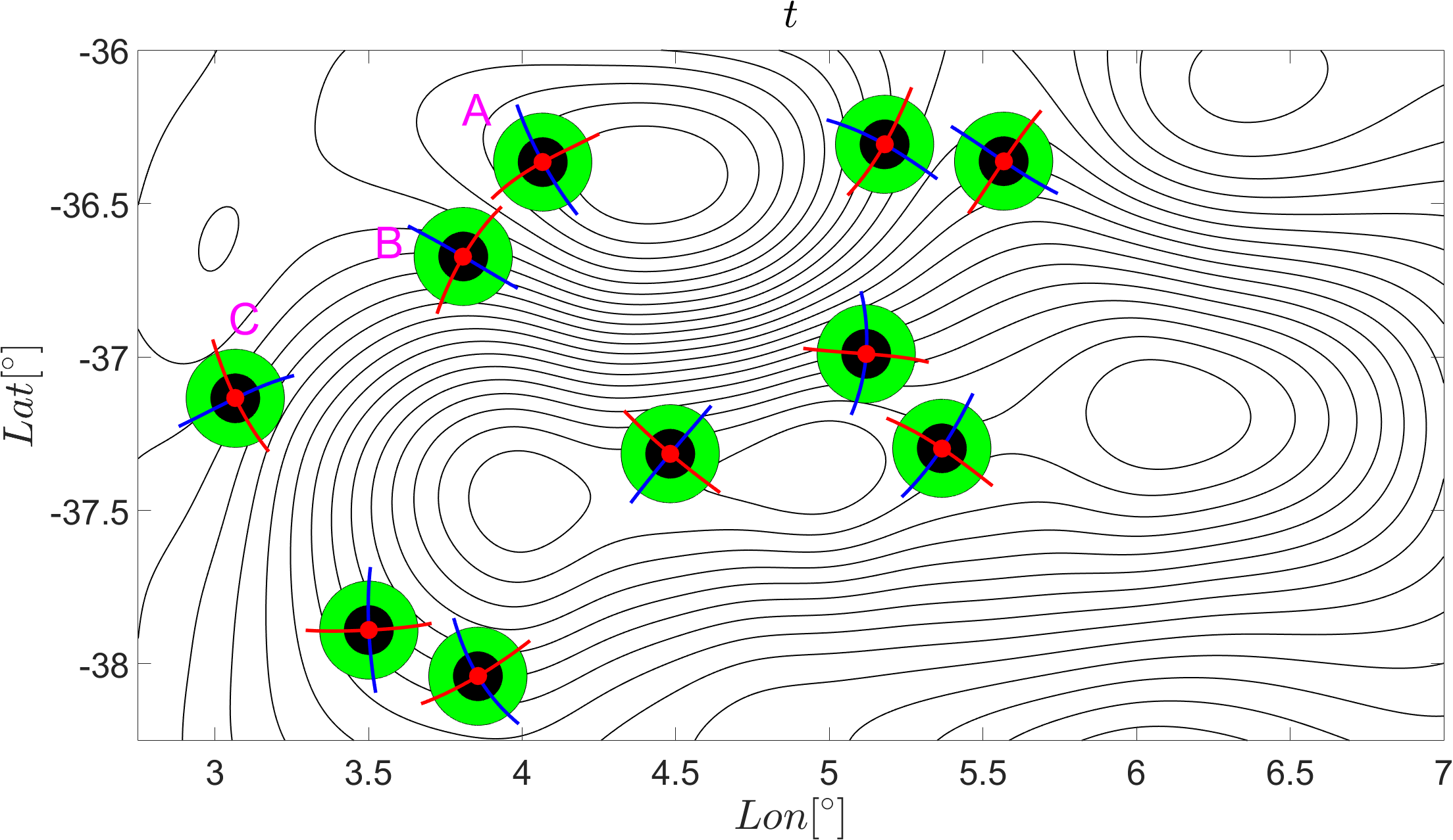
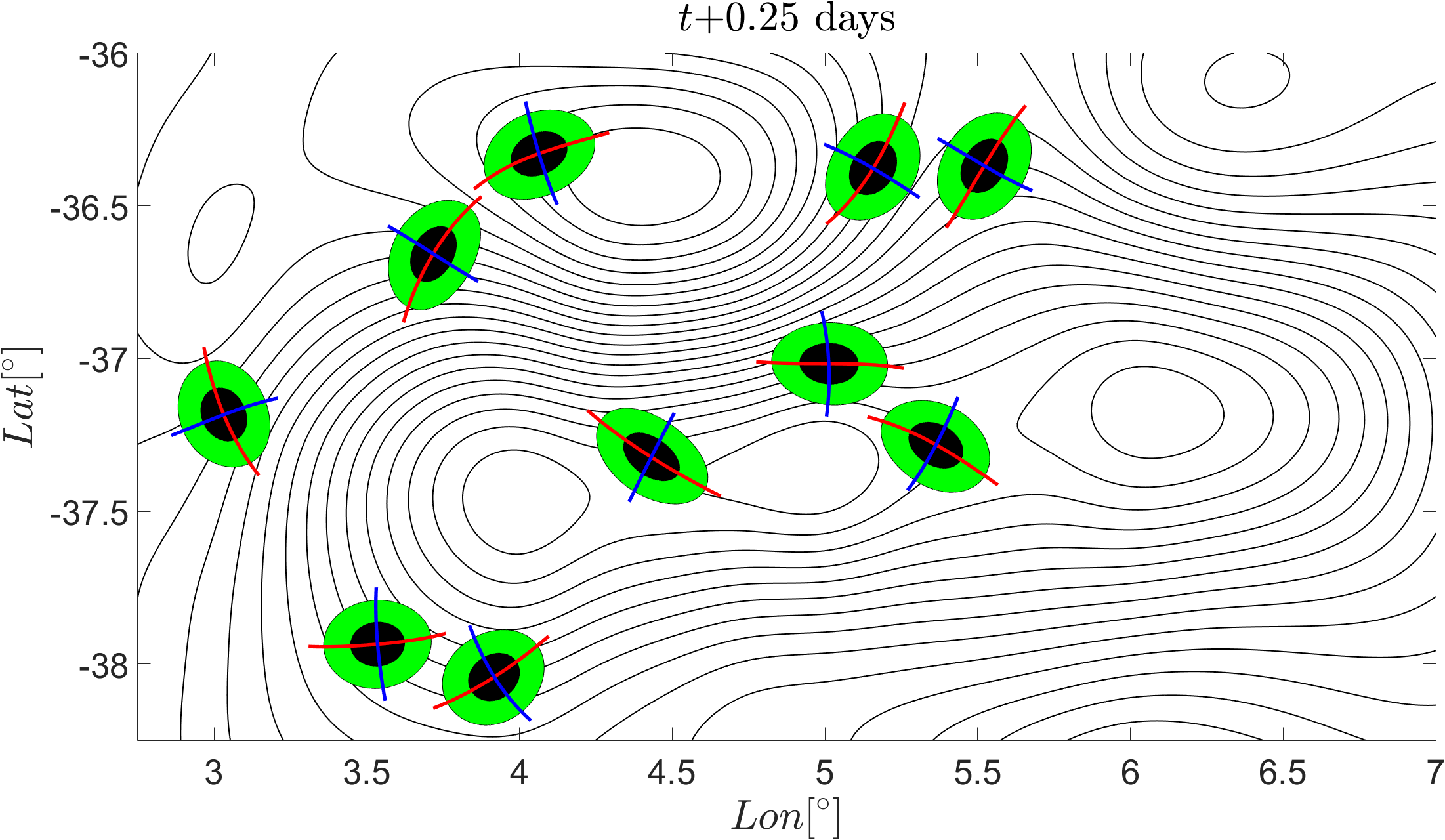
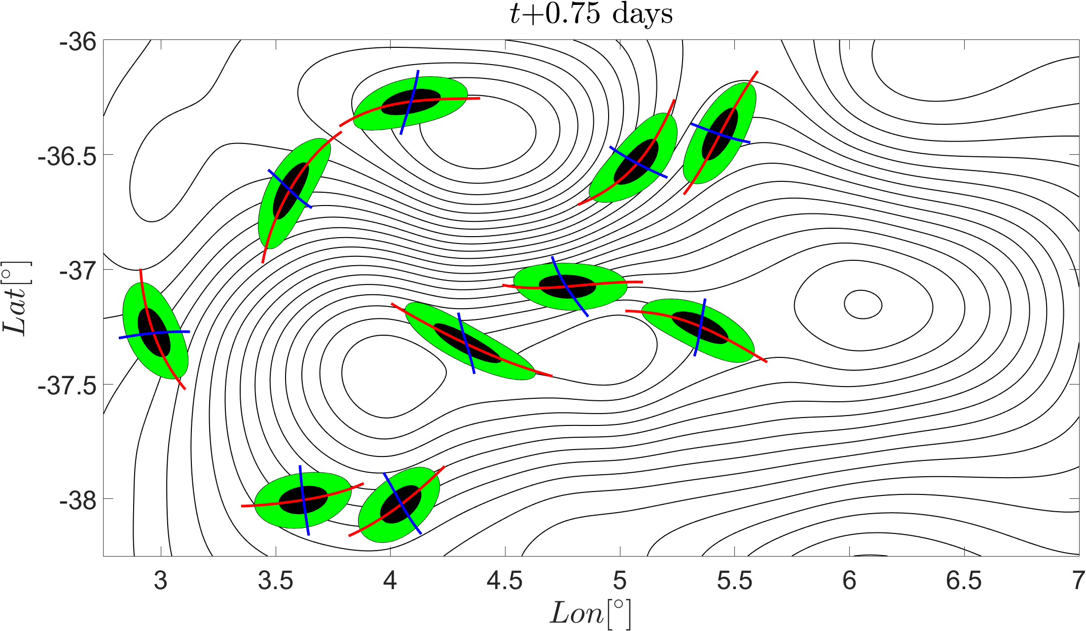
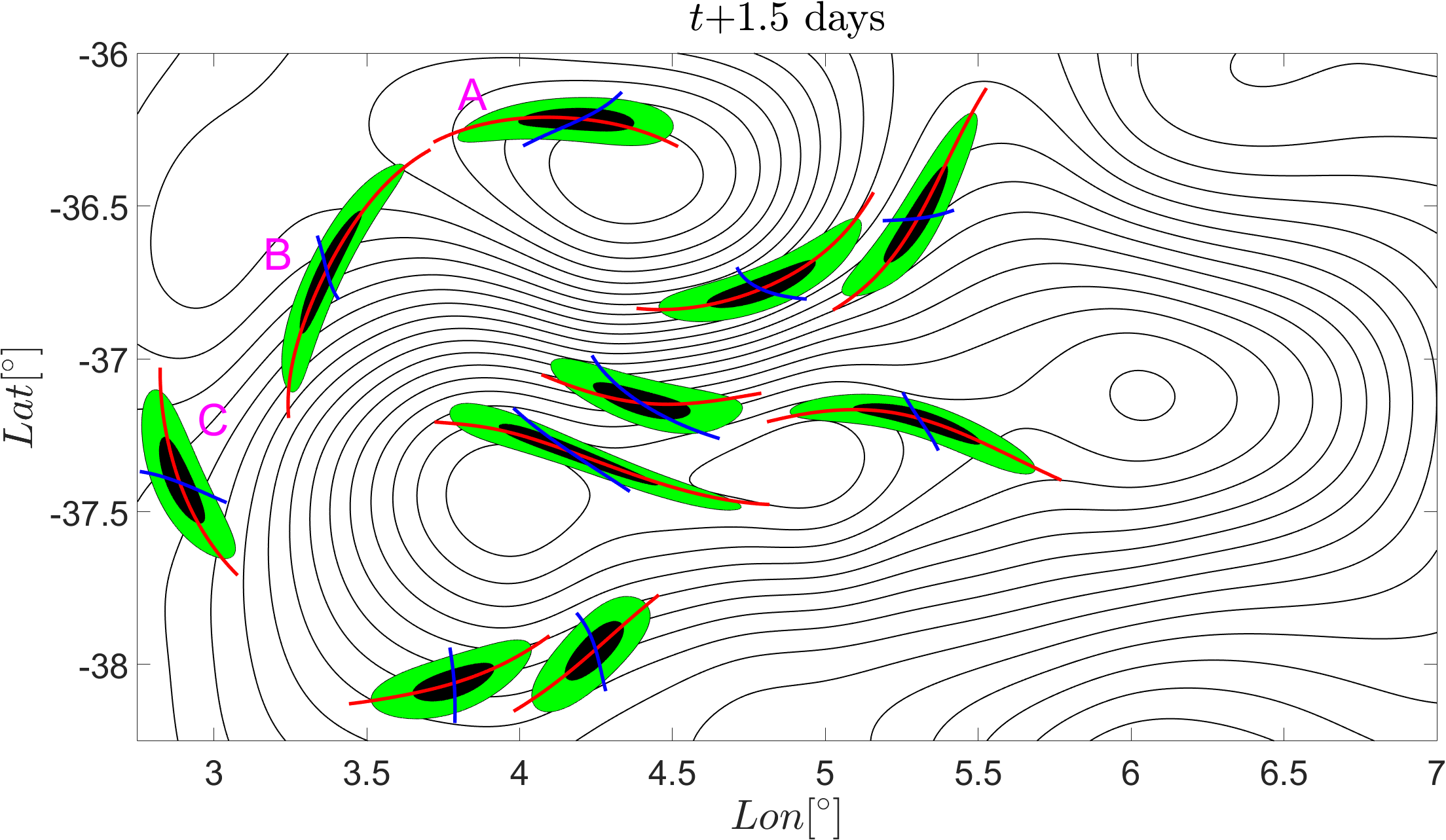
Figure 10 shows how hyperbolic OECSs act as instantaneous stable and unstable manifolds for short-term particle motion. Remarkably, several hyperbolic OECSs cross the local streamlines at large angles at the initial time (Fig. 10a), as well as at later times (Figs. 10b-10d), explaining the deformation of nearby blobs of fluid. In particular, the objective saddle point (cf. Remark 1) captured by a hyperbolic OECS (point A in Figs. 10a, 10d) induces markedly hyperbolic short-term Lagrangian behavior even though it is located within an area of closed streamlines. In a similarly surprising fashion, the objective saddle points B and C create significant short-term material stretching in a direction perpendicular to the local streamlines.
Figure 11 presents the same results as Fig. 10d but over level sets of the the negative Okubo–Weiss parameter . Note how some hyperbolic OECSs cross closed contours around local minima of that are generally believed to signal elliptic regions.
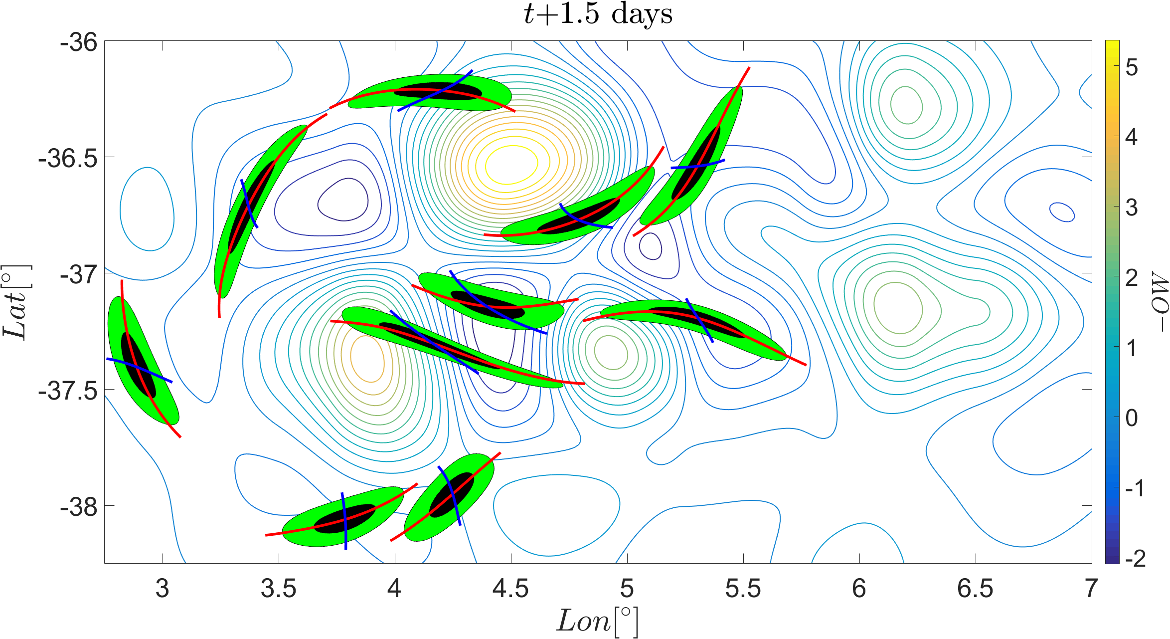
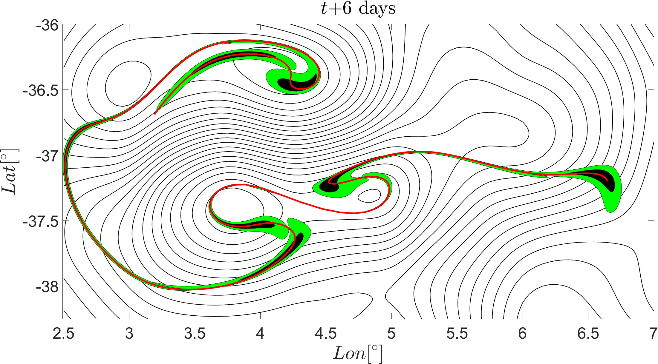
Figure 12 illustrates that attracting OECSs continue to shape short-term tracer deformation patterns in larger distances from their cores, for times up to six days. Over this time interval, material blobs align with materially advected -lines, underlining the role of attracting OECSs as short-term unstable manifolds.

A common Eulerian diagnostic for short-term hyperbolic tracer behavior is the identification of instantaneous saddle-type stagnation points in the velocity field. For comparison with this diagnostic, we show in Fig. 13a the only three saddle-type stagnation points (magenta triangles) that exist instantaneously in the domain at time . Also shown are the corresponding stable (dash blue) and unstable (dash red) directions inferred from streamlines (black lines) for these stagnation points, along with the ten objective saddle points (red dots) found at the same time instant.

Two of these red dots marking hyperbolic OECS cores in Fig. 13 fall near two instantaneous stagnation points, and give an improved objective prediction for the cores of short-term saddle-type behavior in Lagrangian particle motion. The improvement is seen by tracking the deformation of the advected fluid blobs, initially centered on the stagnation points. These blobs must stretch as they lie close to two objective saddle points. The stretching blobs, however, align more closely with the advected -lines shown in Fig. 10 when compared to the advected streamline segments shown in Fig. 13. The instantaneous stagnation point on the top left, instead, induces no notable material stretching on nearby particles since there are no hyperbolic OECS cores in its vicinity. The remaining eight hyperbolic OECSs remain completely hidden in the instantaneous streamline picture (cf. Fig. 13), even though they induce significant saddle-type material stretching, as we have already seen in Fig. 10.
These results illustrate that an instantaneous forecast strategy based
on saddle-type stagnation points of the velocity field may miss the
majority of significant short-term material stretching events in the
flow. Even for the detected stagnation points, there is no guarantee
that they signal nearby Lagrangian hyperbolic behavior correctly,
unless the velocity field has slow enough variation in their vicinity
[20]. This mismatch between objective and frame-dependent
predictions for saddle points is generally expected to increase further
for highly unsteady flows.
8.3 Parabolic OECSs
We now discuss the existence of parabolic OECSs in the full domain used for computing elliptic OECSs. There is no known persistent Eulerian or Lagrangian jet in this part of the ocean, but we nevertheless uncover parabolic OECSs in this region that act as short-term pathways for material transport.
In Fig. 14, we show three parabolic OECSs obtained from the application of Algorithm 4 to the velocity data studied here. These OECSs are, therefore, alternating chains of -lines (blue) and -lines (red), connecting trisector-type (blue dots) singularities and wedge-type singularities (black dots), with the streamlines shown in the background for reference. The three parabolic OECSs are of approximate sizes km for and km for and .
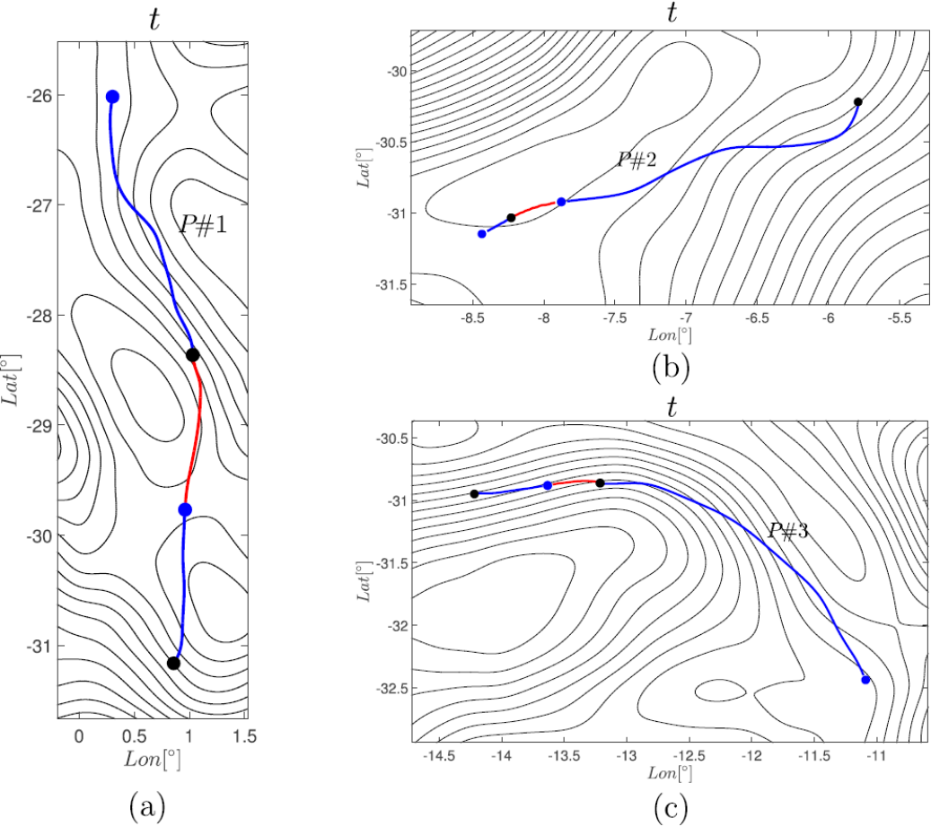
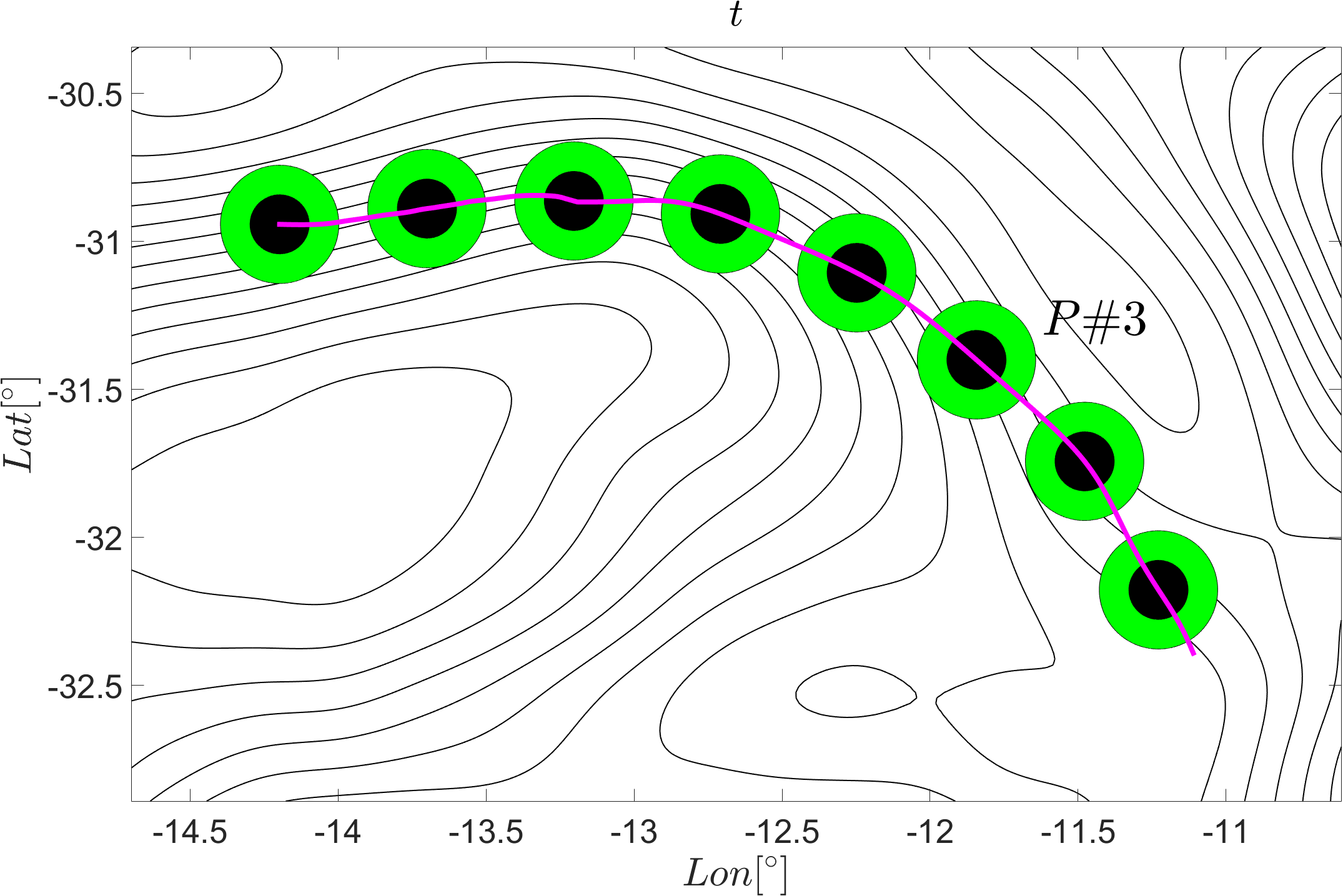
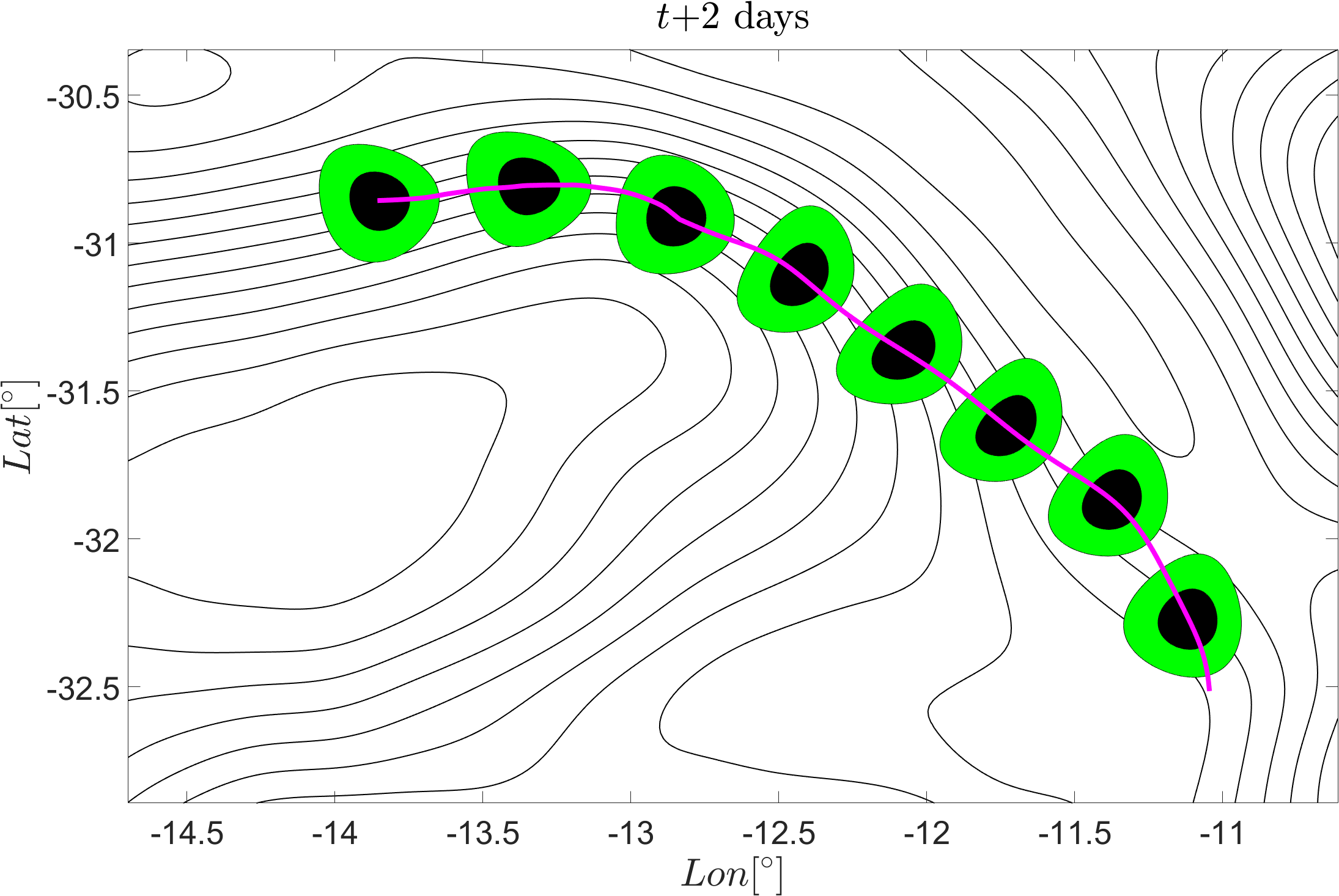
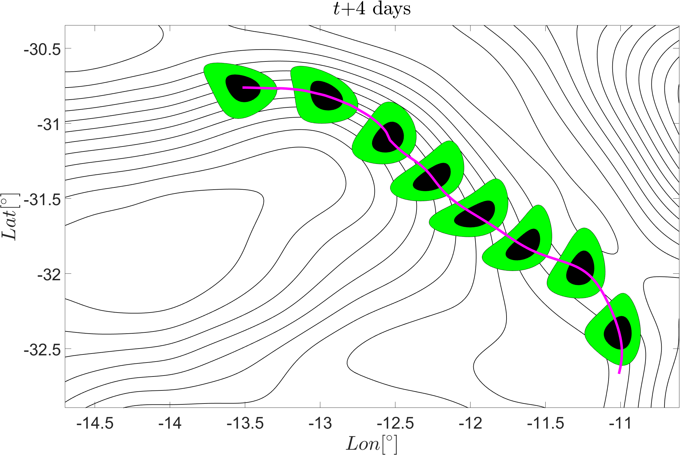
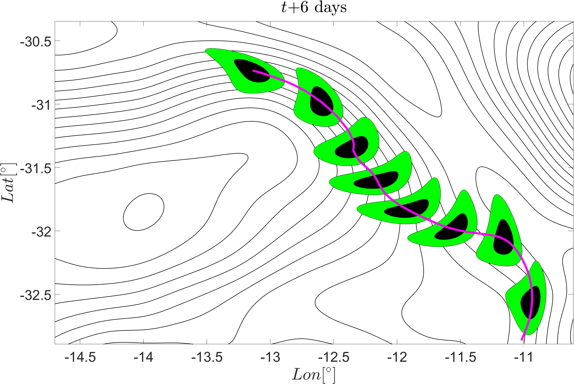
As a representative example, Fig. 15 shows the advected positions of the parabolic OECS, P#3, along with the deformation of material blobs initialized along this OECS, for integration times up to six days. The advection illustrates the existence of a short-term pathway along which initial conditions march towards the bottom right. The deformation of the blobs has a characteristic boomerang shape, which is similar to that observed along persistent Lagrangian jets [10, 14]. This objective short-term transport route, therefore, has a clearly verifiable material impact even though it has no clear signature in the instantaneous streamline geometry.
9 Conclusions
We have developed a variational theory of objective Eulerian Coherent Structures (OECSs) for two-dimensional, non-autonomous dynamical systems. In this theory, we define OECSs at time as curves with the lowest instantaneous material stretching rate or shearing rate in the flow. We defined elliptic OECSs as closed stationary curves of the instantaneous stretching-rate and shearless OECSs as stationary curves of the instantaneous shearing-rate functional. A further classification of shearless OECSs divides them into hyperbolic (attracting or repelling) and parabolic (jet-type) OECSs. The approach we have taken here is objective, i.e., returns the same OECSs in frames translating and rotating relative to each other.
In our present, instantaneous context, objectivity guarantees a self-consistent detection of short-term material coherent structures via OECSs in unsteady, two-dimensional fluid flows. Indeed, we have shown that elliptic OECS provide accurate identification of short-term material vortices; hyperbolic OECSs reveal generalized saddle points with the corresponding stable and unstable manifolds; and parabolic OECSs uncover short-term jet-type pathways for material transport. We have verified the accuracy of these OECS-based predictions by actual material advection in our ocean data example obtained from satellite altimetry.
We have also compared our results to other broadly used instantaneous coherent structure indicators: streamline topology (which is neither Galilean invariant nor objective) and the Okubo–Weiss criterion (which is Galilean invariant but not objective). Such diagnostics often need an ad hoc selection of threshold parameters, which limits the reliability of the results they provide. In contrast, our procedure uses no free parameters or thresholds.
We have found examples of false positives and false negatives suggested by these non-objective Eulerian indicators. For instance, several regions of maximum – ellipticity turn out to stretch significantly more than the regions identified by elliptic OECSs. Even when the indicators happen to suggest an OECS, the objective variational principles developed here give more accurate results, as confirmed by short-term material advection of the detected sets.
As an alternative, elliptic OECSs can also be sought as closed curves showing short-term rotational coherence, i.e., equal material rotation rate [19]. Obtained as the instantaneous limit of a Lagrangian rotational coherence principle, rotationally coherent OECSs are also objective. These OECSs do not restrict stretching rates and hence would generally be expected to give slightly larger but less coherent Eulerian vortices than the ones detected by the approach developed here. Those larger vortices display tangential filamentation, while the stretching-rate-based OECSs introduced here are instantaneous limits of the perfectly coherent, black-hole-type elliptic LCSs derived in [18].
OECS-based forecasting of material transport and mixing is necessarily confined to shorter time scales. Such shorter time scales, however, are precisely the relevant ones for flow control or environmental assessment where quick operational decisions need to be made. Results on the use of OECSs in short-term forecasting and an extension to higher dimensions will appear elsewhere.
Acknowledgment
We would like to acknowledge Mohammad Farazmand for helpful discussions on the subject of this paper.
Appendix A Deformation-rate measures for material curves
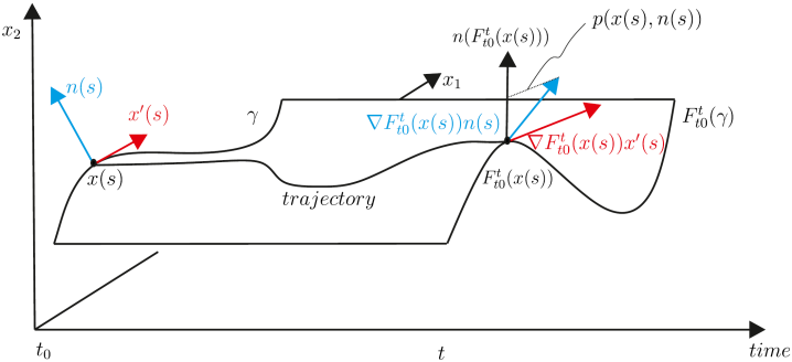
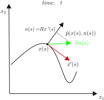
At time , consider a smooth curve of initial conditions , parametrized as via its arclength . Let and denote the local tangent and normal vectors to respectively. While tangent vectors of are mapped into tangent vectors by the linearized flow map , initial normal vectors at time are not mapped by into the normal space at time (Fig. 16a). The local deformation of and its nearby trajectories, over the time interval , can be expressed in terms of two Lagrangian quantities: the tangential shear and the tangential strain over the time interval (see [10] and [18]).
Specifically, the tangential shear at point is given by
and the tangential strain at the same point is give by
The quantities and give pointwise information on tangential shear and tangential stretching experienced by a material curve over the time interval in an objective (frame-invariant) fashion.
The instantaneous rates of shear and tangential stretching along can be obtained by differentiating and with respect to and setting . Specifically, we have
and
where we used the following relations
| (24) | ||||
Appendix B is a one-parameter family of rotated vector fields
Assume there exists a limit cycle of (16), , for one choice of and a fixed value of . The hyperbolic nature of limit cycles guarantees their persistence with respect to small changes in the parameter , which leads to a one-parameter family of limit cycles for the vector field . In general, these limit cycles can deform in an arbitrary fashion and even intersect each other.
In the present case, however, turns out to be as a one-parameter family of rotated vector fields in the sense of [9]. This means that trajectories of (16), for each of the choices , cannot intersect when varies and shrink or expand for monotonic changes of the parameter. Hence, limit cycles of one-parameter family of rotated vector fields, corresponding to different values of , cannot intersect each other.
To qualify as a one-parameter family of rotated vector fields, must be locally smooth in a neighborhood of the limit cycle, and the vector field defined by must keep the same orientation with respect to the plane spanned by and .
Indeed, is smoothly orientable in the vicinity of limit cycles, although it is not globally orientable due to orientational discontinuities of the fields. For the second condition above, it is equivalent to check that , with denoting the planar unit vector, remains unaltered over the domain for each of the choices .
In the basis, can be computed as
therefore, keeps the same orientation for each of the signs , under a monotonic change of the parameter .
With our choice of relative orientation between and , (cf. equation (4)), the sign of gives the direction of rotation (positive counterclockwise) of the field when the parameter increases, for each of the choices . Finally, the quantity could be used in the computation of Elliptic OECSs through a systematic change of the parameter , as described in [18].
References
- [1] M. R. Allshouse and J. L. Thiffeault. Detecting coherent structures using braids. Physica D, 241:95–105, 2012.
- [2] J. K. Beem, P. L. Ehrlich, and L. E. Kevin. Global Lorentzian Geometry. CRC Press, 1996.
- [3] F. J. Beron-Vera, Y. Wang, M. J. Olascoaga, G. J. Goni, and G. Haller. Objective detection of oceanic eddies and the Agulhas leakage. J. Phys. Oceanogr., 43:1426–1438, 2013.
- [4] G. Boffetta, G. Lacorata, G. Redaelli, and A. Vulpiani. Detecting barriers to transport: a review of different techniques. Physica D, 159:58–70, 2001.
- [5] M. Budišić and I. Mezić. Geometry of the ergodic quotient reveals coherent structures in flows. Physica D, 241:1255–1269, 2012.
- [6] P. Chakraborty, S. Balachandar, and R. J. Adrian. On the relationships between local vortex identification schemes. J. Fluid Mech., 535:189–214, 2005.
- [7] T. Delmarcelle. The Visualization of Second-Order Tensor Fields (Ph. D. Thesis). 1994.
- [8] T. Delmarcelle and L. Hesselink. The topology of symmetric, second-order tensor fields. In Proceedings of the conference on Visualization ’94, pages 140–147. IEEE Computer Society Press, 1994.
- [9] G. F. D. Duff. Limit-cycles and rotated vector fields. Ann. Math., pages 15–31, 1953.
- [10] M. Farazmand, D. Blazevski, and G. Haller. Shearless transport barriers in unsteady two-dimensional flows and maps. Physica D, 278:44–57, 2014.
- [11] M. Farazmand and G. Haller. Computing Lagrangian coherent structures from their variational theory. Chaos, 22:013128, 2012.
- [12] M. Farazmand and G. Haller. Erratum and addendum to “A variational theory of hyperbolic Lagrangian coherent structures” [Physica D 240 (2011) 574–598]. Physica D, 241:439–441, 2012.
- [13] G. Froyland and K. Padberg-Gehle. Almost-invariant and finite-time coherent sets: directionality, duration, and diffusion. In Ergodic Theory, Open Dynamics, and Coherent Structures, pages 171–216. Springer, 2014.
- [14] A. Hadjighasem and G. Haller. Geodesic Transport Barriers in Jupiter’s Atmosphere: A Video-Based Analysis. arXiv preprint arXiv:1408.5594, 2014.
- [15] G. Haller. An objective definition of a vortex. J. Fluid Mech., 525:1–26, 2005.
- [16] G. Haller. A variational theory of hyperbolic Lagrangian coherent structures. Physica D, 240:574–598, 2011.
- [17] G. Haller. Lagrangian coherent structures. Annual Rev. Fluid. Mech, 47:137–162, 2015.
- [18] G. Haller and F. J. Beron-Vera. Coherent Lagrangian vortices: the black holes of turbulence. J. Fluid Mech., 731, 9 2013.
- [19] G. Haller, A. Hadjighasem, M. Farazmand, and F. Huhn. Defining Coherent Vortices Objectively from the Vorticity. arXiv preprint arXiv:1506.04061, 2015.
- [20] G. Haller and A. Poje. Finite time transport in aperiodic flows. Physica D, 119:352–380, 1998.
- [21] J. Jeong and F. Hussain. On the identification of a vortex. J. Fluid Mech., 285:69–94, 1995.
- [22] D. Karrasch, F. Huhn, and G. Haller. Automated detection of coherent Lagrangian vortices in two-dimensional unsteady flows. In Proc. R. Soc. Lond. A., volume 471. The Royal Society, 2015.
- [23] G. Lapeyre, B. L. Hua, and B. Legras. Comment on “finding finite-time invariant manifolds in two-dimensional velocity fields”. Chaos, 11:427–430, 2001.
- [24] G. Lapeyre, P. Klein, and B. L. Hua. Does the tracer gradient vector align with the strain eigenvectors in 2D turbulence? Phys. Fluids, 11:3729–3737, 1999.
- [25] H. J. Lugt. The dilemma of defining a vortex. In Recent developments in theoretical and experimental fluid mechanics, pages 309–321. Springer, 1979.
- [26] T. Ma and E. M. Bollt. Differential geometry perspective of shape coherence and curvature evolution by finite-time nonhyperbolic splitting. SIAM J. Appl. Dyn. Syst., 13:1106–1136, 2014.
- [27] A. Okubo. Horizontal dispersion of floatable particles in the vicinity of velocity singularities such as convergences. In Deep-Sea Res., volume 17, pages 445–454. Elsevier, 1970.
- [28] T. Peacock and J. Dabiri. Introduction to focus issue: Lagrangian coherent structures. Chaos, 20:017501, 2010.
- [29] T. Peacock, G. Froyland, and G. Haller. Introduction to Focus Issue: Objective Detection of Coherent Structures. Chaos, 25:087201–087201, 2015.
- [30] A. Provenzale. Transport by coherent barotropic vortices. Annual Rev. Fluid. Mech, 31:55–93, 1999.
- [31] M. Tabor and I. Klapper. Stretching and alignment in chaotic and turbulent flows. Chaos, Solitons & Fractals, 4:1031–1055, 1994.
- [32] C. Truesdell and W. Noll. The non-linear field theories of mechanics. Springer, 2004.
- [33] J. Weiss. The dynamics of enstrophy transfer in two-dimensional hydrodynamics. Physica D, 48:273–294, 1991.