Obtaining A Linear Combination of the Principal Components of a Matrix on Quantum Computers
Abstract
Principal component analysis is a multivariate statistical method frequently used in science and engineering to reduce the dimension of a problem or extract the most significant features from a dataset. In this paper, using a similar notion to the quantum counting, we show how to apply the amplitude amplification together with the phase estimation algorithm to an operator in order to procure the eigenvectors of the operator associated to the eigenvalues defined in the range , where and are real and . This makes possible to obtain a combination of the eigenvectors associated to the largest eigenvalues and so can be used to do principal component analysis on quantum computers.
I Introduction
Principal component analysis (PCA) is widely used as a multivariate statistical technique to reduce the dimension of a problem or to extract most important features from high dimensional datasets by fitting ellipsoids representing principal components to the given dataset F.R.S. (1901); Jolliffe (2002). Examples of PCA with different descriptions and settings include probabilistic PCA Tipping and Bishop (1999), nonlinear PCA de Leeuw (2005), kernel PCA Schölkopf et al. (1997) as a nonlinear extension of PCA, local PCA Kambhatla and Leen (1997) for dimension reduction, and generalized PCA Vidal et al. (2005), applied to a wide variety of problems in science and engineering Jolliffe (2002): e.g., it is a prevalent method in pattern recognition Bishop (2006). Principal component analysis best explains the variation in the whole dataset represented by an matrix representing observations described by variables. For a set of data vectors, in PCA, one finds orthonormal axes describing a linear projection of the dataset under which the retained variance is maximum. These orthonormal axes-so called the principal components-corresponds to the dominant eigenvectors associated with the largest eigenvalues of the covariance matrix. The projection onto the subspace spanned by these eigenvectors not only eliminates the possible noise in the data but reduces the size of the original high dimensional data as well Tipping and Bishop (1999). To obtain the eigenvectors corresponding to the largest eigenvalues, generally singular value or eigenvalue decomposition techniques are applied to the matrix or to the covariance matrix . For unfamiliar readers, we recommend the simple introductory tutorial given in Ref. Shlens (2014) and the book in Ref.Jolliffe (2002) for further information on PCA and its applications.
Eigenvalue related problems can be solved successfully on quantum computers by using the well-known quantum phase estimation algorithm (PEA) Kitaev (1996). Given an input initial approximate eigenvector, PEA generates the associated eigenvalue in a more efficient way than all the known classical algorithms Papageorgiou et al. (2013). However, finding a good approximate initial state required for the algorithm is a nontrivial task which inevitably impinges on the efficiency. PEA with an equal superposition state is shown to eliminate the need for an approximate initial eigenvector for obtaining the eigenvector associated with the largest eigenvalue of a stochastic matrix Daskin et al. (2014a); Daskin (2015). PEA is also applied to solve the linear systems of equations given in the form . In that case, the initial state is mapped to the vector and the solution is obtained as the final state. In addition, it is shown that a flag register can be used to eliminate the ill-conditioned part of and process only eigenvalues greater than some threshold value Harrow et al. (2009).
Research in quantum algorithms proposed for machine learning and analyses of big data have gained a lot of momentum in recent years (e.g. see Rebentrost et al. (2014); Wittek (2014); Schuld et al. (2014)). Speed-ups over the conventional classical methods are shown to be achievable mostly by using adiabatic quantum computation Neven et al. (2008, 2009) or mapping data set to quantum random access memory Aïmeur et al. (2013); Lloyd et al. (2014a). Furthermore, in Ref.Lloyd et al. (2014b), Lloyd et al. have described a method for quantum principal component analysis: In their method, multiple copies of a quantum system defined by the low rank density matrix are used to obtain efficiently. Then, the phase estimation algorithm with the initial state itself is applied to generate a final quantum state , where s, s and s are respectively the eigenvalues, the eigenvectors and the estimates of the eigenvalues of . Sampling from this final quantum state, one is obviously able to obtain any of the eigenvectors. In addition, when is a low rank matrix, they have showed that the final state is in superposition of the principal eigenvectors, which can be used in the principal component analysis.
In this paper, we present a different general framework to do principal component analysis on quantum computers by showing how to generate the eigenvalues defined in certain range and their corresponding eigenvectors in the phase estimation algorithm. In particular, as done in Ref. Daskin et al. (2014a); Daskin (2015), we first use the phase estimation algorithm with an initial superposition state to generate an output state which has the superposition of the eigenvalues of a given operator on the first register and the associated eigenvectors on the second register. We then show how to apply the amplitude amplification to this output state to amplify the amplitudes of the desired eigenvalues and their associated eigenvectors. We then give a numerical example and finally discuss the future research directions.
II Preliminaries
II.1 Quantum Phase Estimation Algorithm
When there exists an initial estimate for the eigenvector of a operator , PEA finds the associated eigenvalue by using the powers of the time evolution operator . PEA consists of two registers: the first register, , holds the eigenvalue at the end with the precision determined by the number of qubits, , allocated for this register. On the other hand, with number of qubits is used for the eigenvector. The algorithm starts with the initial state =, where is the eigenvector associated to , the th eigenvalue of . It then applies to the initial state. Here, describes a quantum operation: controlled by the th qubit in the first register and applied to the second register. And and are respectively the quantum Fourier and inverse Fourier transforms applied to the first register. The final quantum state holds the eigenvalue on the first register and the associated eigenvector on the second register:
| (1) |
Therefore, measuring the first register produces with the precision determined by the number of qubits in the first register.
II.2 Quantum Amplitude Amplification
Grover’s search algorithm Grover (1998) can be applied to amplify the amplitude of a solution encoded in a quantum state. Consider an quantum operator (or an algorithm) mapping an initial quantum state into Mosca et al. (1998); Brassard et al. (2002); Kaye et al. (2006):
| (2) |
where s are the complex amplitudes, represents the th vector in the standard basis, and is considered as some “junk” state or additional workspace (This state shall be used for the eigenvector in the next section.). From this equation, the probabilities to see the “good” and the “bad” states described by the sets and , respectively, are as follows:
| (3) |
When these probabilities inside (0,1), i.e. , an orthonormal basis set for two dimensional subspace can be formed by separating and renormalizing the “good” and the “bad” components of the state in Eq.(2):
| (4) |
In terms of the orthonormal basis , Eq.(2) can be rewritten as:
| (5) |
where for .
It is known that to amplify the amplitude of the searched item, the search iterate described by the following matrix product can be used:
| (6) |
When the operators in the above applied to , they acts as follows: negates the amplitude of the searched item (the “good” states) and does nothing for the other items (the “bad” states):
| (7) |
In addition, the operator can be constructed by considering it as the reflection about the state :
| (8) |
where is the identity matrix. in Eq.(6) is the reflection about the axis defined by the vector : . And so the operator in Eq.(6) reads the following:
| (9) |
Note that this is also a reflection operator: when is applied to , it does nothing. However, it changes the sign of the states, , orthogonal to :
| (10) |
Consequently, the application of to rotates the state in the following way:
| (11) |
For , this obviously increases the magnitude of the amplitude of the state . For the number of repeated applications of , the final state reads:
| (12) |
The highest probability occurs when , which allows to be bounded by . Since when is small, we can conclude that the required number of iterations for the maximum probability is approximately , i.e., .
III Quantum Principal Component Analysis
In this section, we shall show how to use PEA and amplitude amplification to obtain the eigenvectors corresponding to the largest eigenvalues of an operator.
Consider that the eigenvalues of the operator are ordered as . In the principal component analysis, we deal with the eigenvectors associated with the first principal eigenvalues. Accordingly, in the phase estimation algorithm, we need to find a way to produce a quantum state in which the first register is the superposition of the first eigenvalues while the second register represents the superposition of the associated eigenvectors. When the initial state in the phase estimation algorithm is in a superposition state, PEA generates the superposition of the eigenvectors and the eigenvalues with the amplitudes defined by the overlap of the eigenvectors with the initial superposition state.
To get a quantum state which is the superposition state of these eigenvectors, we first define a range with expected to include the principal eigenvalues. Here, one can define a controlled measurement operator to get the state in the second register where the value of the first register falls in the range . However, in the cases when the initial state is almost orthogonal to the eigenvectors; the success probability gets very low since it depends on the overlap of the eigenvectors and the initial state.
Instead of a controlled measurement; following a similar notion to the well-known quantum counting Mosca (2001), here, we apply the amplitude amplification to the output of the phase estimation algorithm: first, the eigenvalues lying in this range are marked and then, their amplitudes are amplified. In this amplification process, two operators are needed: one is to mark the desired amplitudes and the other one is to amplify the amplitude of the marked item. In the following subsection, we describe this process in detail in two parts: viz, the phase estimation part and the amplitude amplification part.
III.1 Details of the Method
III.1.1 The Phase Estimation Part
The first part of the method follows the standard phase estimation algorithm with the initial equal superposition state. The transition of the states in this part is as follows:
III.1.2 The Amplitude Amplification Part
The second part of the method is the amplitude amplification part where the desired eigenvalues are first marked by the operator , and then the amplitudes corresponding to those eigenvalues are amplified by the application of the operator . While is applied only to the first register, is applied to the whole system. This is summarized as follows:
Note that if there are more than one marked item: i.e. the first number of eigenvalues are marked, then the success probability at the end of the phase estimation part is the following:
| (20) |
Therefore, the required maximum number of runs is bounded by
| (21) |
III.2 The Circuit Implementation
The circuit for the phase estimation part of the algorithm represented by the operator is the same as the well known circuit for the phase estimation procedure (see the related chapter in Ref.Kaye et al. (2006)). In addition to , the implementation of the whole algorithm requires and :
is a logical operation that marks the eigenvalue if it is greater (or less) than the bounds of the given range. It operates only on the first register and defined in the following form
| (22) |
where is the number of qubits and defines which states to be marked. For instance, to mark the states corresponding to the phases greater than 0.5, we first form in a way that 1 is put to the states which gives a value greater than 0.5 and normalize the formed vector. For m=3, the obtainable quantum states and the phase values are: =1, =0.125, =0.25, =0.375, =0.5, =0.625, =0.750, =0.875. Therefore, we define and use Eq.(22) to obtain the reflection operator . marks only the states corresponding to eigenvalues since the other states does not exist in the superposition: if, for instance, the eigenvalues of the operator greater than 0.5 are 1 and 0.75, then only the states corresponding to these values are marked. Also note that is a special case of the general Householder transformation (or reflection). Householder transformations are used as ingredients to simulate arbitrary unitary matrices Bullock et al. (2005); Ivanov et al. (2006); Urías and Quiñones (2015); Ivanov and Vitanov (2008) and hence can be efficiently simulatable on quantum computers.
The operator is also a reflection, the same as the diffusion operator used in the Grover’s algorithm, and can be simulated by using a controlled quantum phase gate.
IV Numerical Example
Here, as an illustrative example, we shall use a simple x system with the eigenvalues chosen as:
| (23) |
The columns of the following random orthogonal matrix are assigned as the eigenvectors of the system associated with the above eigenvalues:
| (24) |
With the initial equal superposition state, the probabilities to see any of the eigenvalues in the output of the phase estimation algorithm are determined by the squares of the normalized sums of the eigenvector elements: i.e. and .
In order to increase the amplitude of the eigenvalue 1 and the associated eigenvector, we first define as:
| (25) |
where . marks the states when the first register is equal to which indicates . We then define :
| (26) |
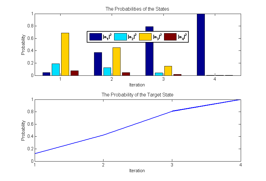
The combination of the above two operators, , is used for the amplitude amplification. After three consecutive applications of , the probability goes to the maximum as shown in Fig.1.
In the second example, we increase the amplitudes of the eigenvalues 1 and 0.75 by defining as follows:
| (27) |
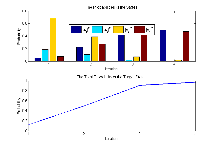
where . In this case, we mark the amplitudes when the first register is in either or states. The same number of the applications of again brings the final state into the superposition of the desired eigenvalues and the eigenvectors: , where and are the amplified amplitudes. The probability changes are shown in Fig.2.
V Discussion and Future Direction
V.1 Determining a Range for the Eigenvalues
The method can be used to study the eigenvectors corresponding to the extremal eigenvalues of an operator by using the upper and lower bounds for these eigenvalues (for the works on the eigenvalue bounds, see e.g. Higham and Tisseur (2003); Persi Diaconis (1991); Wu (2005)). It can also be used to study the eigenvectors corresponding to a group of eigenvalues for which the upper and the lower limits are known. Maximum eigenvalue of a matrix lies between the maximum and minimum column sums due to the correlation of the different matrix norms. There are also different bounds for the eigenvalues in specific problems.
One of the methods which can be used to determine bounds for eigenvalues is the Gershgorin theorem Wilkinson (1965); Stewart (1975): For the each th column ( or row) of a complex matrix, a Gershgorin disc is defined by assigning the diagonal entry on the th column as the center and the absolute sum of the non-diagonal elements thereof as the radius. The Gershgorin theorem indicates that every eigenvalue of the matrix lies within at least one of such discs. And the union of number of discs disjoint from the rest contains exactly number of eigenvalues. As a result, the eigenvalues lies within the certain range determined from these discs can be used in the method to study the corresponding eigenvectors.
V.2 Number of Iterations
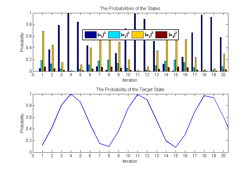
Determining the right number of iterations is one of the most important requirement for the success of the method since the success probability for the desired states oscillates by the applications of the amplitude amplification. This oscillation is shown in Fig.3, where the probability becomes maximum after four applications of the amplitude amplification but then it starts to oscillate.
The number of iterations in the amplitude amplification part is determined by , where is the amplitude of the desired quantum state. The amplitudes, s, at the end of the phase estimation algorithm are the sum of the eigenvector elements. Therefore, without knowing the eigenvector components, it is impossible to know exact amplitudes.
However, there exists a method called QSearch (Quantum Search) for searching without knowing the success probabilities Kaye et al. (2006). In our case, QSearch can be used as follows: After every iteration of the amplitude amplification, the first register holding the superposition of the eigenvalues is measured. If the measurement result is a value in the range used to construct , the superposition of the desired eigenvectors is successfully formed on the second register. If it is not in the range, then we apply the amplitude amplification again. If there is no desired output obtained in the number of applications, then we conclude that there is no eigenvalue falling in the range . Note that this algorithm uses iterations instead of . Also note that this can also be used to estimate an eigenvalue, given that it is the only eigenvalue in the defined range.
V.3 Differences to the Classical PCA
In classical PCA, one obtains the most significant number of eigenvalues and do the analysis on the obtained associated principal eigenvectors by using some weighted or unweighted combination of these eigenvectors either in matrix or in vector forms. In some sense, the sum of the largest eigenvalues are maximized (or the sum of the rest of the eigenvalues are minimized.). Therefore, for different choice of , PCA describes a different maximization or minimization problem de Leeuw (2005).
However, in the quantum case, instead of number of principal eigenvectors, we deal with the ones associated with the eigenvalues defined in a range. For instance, if all the eigenvectors are less than one, we can choose the eigenvectors greater than 0.75. In some sense, we maximize the sum of the eigenvalues falling into the defined range, which describes a maximization problem similar to but not quite the same as the classical case. Therefore, a different choice of the lower limit for the eigenvalues would describe a different maximization problem. Using some eigenvalue bounds and properties, e.g. the Gershgorin theorem, we may also be able to determine the number of eigenvalues falls in the defined range.
In addition, here, we find the combination of the eigenvectors in the given range rather than number of largest eigenvalues as in the classical PCA. As explained above, this defines a slightly different maximization problem than the classical PCA. Thus, the comparison analyses of the applications of the quantum and the classical PCAs to different problems are necessary. The superposition of the eigenstates obtained in the quantum case can also be considered as the weighted linear combination of the eigenvectors in which the weights are determined by the initial amplitudes s.
V.4 Application to data
In this paper, we have assumed the operator and its power can be efficiently implementable. In PCA, the dimension of the data is generally very high. When the Hamiltonian, , in is sparse, it is known that can be simulated in polynomial time in the number of qubits Berry et al. (2007); Childs and Kothari (2011). This is generally not the case for dense matrices. Nonetheless, efficient implementation methods which are specific to some applications may be described. For instance, if the dataset can be represented as a sum of simple commuting terms, then the circuit for each term can be found easily. However, this ease of representation is not expected to be exactly attainable in the majority of cases. A frequently used method to attain an approximate time-evolution operator of an Hamiltonian is the Trotter-Suziki decomposition Trotter (1959); Suzuki (1976). In the decomposition, while the required number of gates is at least as many as the number of terms used in the Hamiltonian, the error in the approximation increases as some power of the number of terms Poulin et al. (2015). It is also known that using additional qubits ease the design of a quantum circuit for a given operator (e.g. see Daskin et al. (2012, 2014b)). In the possible application, a solution may be obtained on the chosen some substate with the help of additional qubits.
V.5 Processing the Output State
Obtaining a quantum state is not a trivial task. To get meaningful information from the quantum state or process the output state on quantum computers, one can benefit from different measurement schemes: e.g. in Ref. Daskin (2015), we have described a method for the alignment of protein-protein interaction networks and showed how to extract the solution of the alignment efficiently from the measurement statistics: In that case, the largest magnitudes of the amplitudes are sufficient to predict an optimal solution for the alignment. Therefore, some similar schemes can be used for the other problems where extracting the optimal solution from the output state does not require the topology of the whole output state and the significant magnitudes can be used to predict a solution. In some cases, the qubits can also be grouped to use different conditional measurement schemes to obtain meaningful information for the solution.
However, It is known that obtaining the topology of a whole quantum state requires exponential number of computational steps. For the problems whose solutions necessitate the whole vector coefficients, there is a need for research in designing application-specific algorithms to process the obtained quantum eigenstate mostly on the quantum computers.
V.6 Possible Applications
We believe the method described here can be applied to quantum images and may pave the ways to devise algorithms for the applications where principal component analysis is used successfully: e.g. pattern and face recognition.
In Ref.Daskin et al. (2012, 2014b), a general circuit design consisting of qubits and quantum gates is given for the simulation of a matrix of order not necessarily Hermitian. In particular, it is shown that any matrix can be simulated on certain predetermined states by using ancilla qubits. However, although the circuit design method requires only a linear number of computational steps, , the success probability decreases exponentially with the system size, i.e. . Since the states in the simulation are predetermined, the amplitude amplification method described here can also be applied times to the circuit design given in Ref.Daskin et al. (2014b) so as to increase the success probability upto 1. This modification would also increase the complexity, the number of quantum gates, of the circuit to . In addition, a similar modified circuit design may be employed in the principal component analysis to simulate the data matrix.
VI Conclusion
In this paper, we have shown a method by employing the quantum phase estimation algorithm together with the amplitude amplification to obtain the superposition of the principal eigenvectors of a matrix. We have also discussed how to study the eigenvalues defined in a certain range and their corresponding eigenvectors by using this method. Finally, we have shown a numerical example and discussed possible applications. The method paves the way to do principal component analysis on quantum computers.
VII Acknowledgment
This work is supported by TUBITAK under the project number 115E747.
References
- F.R.S. (1901) Karl Pearson F.R.S., “Liii. on lines and planes of closest fit to systems of points in space,” Philosophical Magazine Series 6 2, 559–572 (1901), http://dx.doi.org/10.1080/14786440109462720 .
- Jolliffe (2002) Ian Jolliffe, Principal component analysis (Wiley Online Library, 2002).
- Tipping and Bishop (1999) Michael E Tipping and Christopher M Bishop, “Probabilistic principal component analysis,” Journal of the Royal Statistical Society: Series B (Statistical Methodology) 61, 611–622 (1999).
- de Leeuw (2005) Jan de Leeuw, “Nonlinear principal component analysis,” Department of Statistics, UCLA (2005).
- Schölkopf et al. (1997) Bernhard Schölkopf, Alexander Smola, and Klaus-Robert Müller, “Kernel principal component analysis,” in Artificial Neural Networks—ICANN’97 (Springer, 1997) pp. 583–588.
- Kambhatla and Leen (1997) Nandakishore Kambhatla and Todd K Leen, “Dimension reduction by local principal component analysis,” Neural Computation 9, 1493–1516 (1997).
- Vidal et al. (2005) Rene Vidal, Yi Ma, and Shankar Sastry, “Generalized principal component analysis (gpca),” Pattern Analysis and Machine Intelligence, IEEE Transactions on 27, 1945–1959 (2005).
- Bishop (2006) Christopher M Bishop, Pattern recognition and machine learning (springer, 2006).
- Shlens (2014) Jonathon Shlens, “A tutorial on principal component analysis,” arXiv preprint arXiv:1404.1100 (2014).
- Kitaev (1996) Alexei Kitaev, “Quantum measurements and the Abelian Stabilizer Problem,” Electronic Colloquium on Computational Complexity (ECCC) 3 (1996).
- Papageorgiou et al. (2013) Anargyros Papageorgiou, Iasonas Petras, J Traub, and Chi Zhang, “A fast algorithm for approximating the ground state energy on a quantum computer,” Mathematics of Computation 82, 2293–2304 (2013).
- Daskin et al. (2014a) Anmer Daskin, Ananth Grama, and Sabre Kais, “Multiple network alignment on quantum computers,” Quantum Information Processing 13, 2653–2666 (2014a).
- Daskin (2015) Anmer Daskin, “Quantum isorank: Efficient alignment of multiple ppi networks,” arXiv preprint arXiv:1506.05905 (2015).
- Harrow et al. (2009) Aram W Harrow, Avinatan Hassidim, and Seth Lloyd, “Quantum algorithm for linear systems of equations,” Physical review letters 103, 150502 (2009).
- Rebentrost et al. (2014) Patrick Rebentrost, Masoud Mohseni, and Seth Lloyd, “Quantum support vector machine for big data classification,” Physical review letters 113, 130503 (2014).
- Wittek (2014) Peter Wittek, Quantum Machine Learning: What Quantum Computing Means to Data Mining (Academic Press, 2014).
- Schuld et al. (2014) Maria Schuld, Ilya Sinayskiy, and Francesco Petruccione, “Quantum computing for pattern classification,” in PRICAI 2014: Trends in Artificial Intelligence (Springer, 2014) pp. 208–220.
- Neven et al. (2008) Hartmut Neven, Vasil S Denchev, Geordie Rose, and William G Macready, “Training a binary classifier with the quantum adiabatic algorithm,” arXiv preprint arXiv:0811.0416 (2008).
- Neven et al. (2009) Hartmut Neven, Vasil S Denchev, Geordie Rose, and William G Macready, “Training a large scale classifier with the quantum adiabatic algorithm,” arXiv preprint arXiv:0912.0779 (2009).
- Aïmeur et al. (2013) Esma Aïmeur, Gilles Brassard, and Sébastien Gambs, “Quantum speed-up for unsupervised learning,” Machine Learning 90, 261–287 (2013).
- Lloyd et al. (2014a) Seth Lloyd, Silvano Garnerone, and Paolo Zanardi, “Quantum algorithms for topological and geometric analysis of big data,” arXiv preprint arXiv:1408.3106 (2014a).
- Lloyd et al. (2014b) Seth Lloyd, Masoud Mohseni, and Patrick Rebentrost, “Quantum principal component analysis,” Nature Physics 10, 631–633 (2014b).
- Grover (1998) Lov K Grover, “Quantum computers can search rapidly by using almost any transformation,” Physical Review Letters 80, 4329 (1998).
- Mosca et al. (1998) Michele Mosca et al., “Quantum searching, counting and amplitude amplification by eigenvector analysis,” in MFCS’98 workshop on Randomized Algorithms (1998) pp. 90–100.
- Brassard et al. (2002) Gilles Brassard, Peter Hoyer, Michele Mosca, and Alain Tapp, “Quantum amplitude amplification and estimation,” Contemporary Mathematics 305, 53–74 (2002).
- Kaye et al. (2006) Phillip Kaye, Michele Mosca, and Raymond Laflamme, An introduction to quantum computing (Oxford Univ. Press, UK, 2006).
- Mosca (2001) Michele Mosca, “Counting by quantum eigenvalue estimation,” Theoretical Computer Science 264, 139 – 153 (2001), mFCS’98.
- Bullock et al. (2005) Stephen S Bullock, Dianne P O’Leary, and Gavin K Brennen, “Asymptotically optimal quantum circuits for d-level systems,” Physical review letters 94, 230502 (2005).
- Ivanov et al. (2006) Peter A Ivanov, ES Kyoseva, and NV Vitanov, “Engineering of arbitrary u (n) transformations by quantum householder reflections,” Physical Review A 74, 022323 (2006).
- Urías and Quiñones (2015) Jesús Urías and Diego A Quiñones, “Householder methods for quantum circuit design,” Canadian Journal of Physics 93, 1–8 (2015).
- Ivanov and Vitanov (2008) Peter A Ivanov and Nikolay V Vitanov, “Synthesis of arbitrary unitary transformations of collective states of trapped ions by quantum householder reflections,” Physical Review A 77, 012335 (2008).
- Higham and Tisseur (2003) Nicholas J. Higham and Françoise Tisseur, “Bounds for eigenvalues of matrix polynomials,” Linear Algebra and its Applications 358, 5 – 22 (2003).
- Persi Diaconis (1991) Daniel Stroock Persi Diaconis, “Geometric bounds for eigenvalues of markov chains,” The Annals of Applied Probability 1, 36–61 (1991).
- Wu (2005) Chai Wah Wu, “On bounds of extremal eigenvalues of irreducible and m-reducible matrices,” Linear algebra and its applications 402, 29–45 (2005).
- Wilkinson (1965) James Hardy Wilkinson, The algebraic eigenvalue problem, Vol. 87 (Clarendon Press Oxford, 1965).
- Stewart (1975) Gilbert W Stewart, “Gershgorin theory for the generalized eigenvalue problem 𝐴𝑥= 𝜆𝐵𝑥,” Mathematics of Computation 29, 600–606 (1975).
- Berry et al. (2007) DominicW. Berry, Graeme Ahokas, Richard Cleve, and BarryC. Sanders, “Efficient quantum algorithms for simulating sparse hamiltonians,” Communications in Mathematical Physics 270, 359–371 (2007).
- Childs and Kothari (2011) Andrew M. Childs and Robin Kothari, “Simulating sparse hamiltonians with star decompositions,” in Theory of Quantum Computation, Communication, and Cryptography, Lecture Notes in Computer Science, Vol. 6519 (Springer Berlin Heidelberg, 2011) pp. 94–103.
- Trotter (1959) Hale F Trotter, “On the product of semi-groups of operators,” Proceedings of the American Mathematical Society 10, 545–551 (1959).
- Suzuki (1976) Masuo Suzuki, “Generalized trotter’s formula and systematic approximants of exponential operators and inner derivations with applications to many-body problems,” Communications in Mathematical Physics 51, 183–190 (1976).
- Poulin et al. (2015) David Poulin, MATTHEW B Hastings, Dave Wecker, Nathan Wiebe, Andrew C Doherty, and Matthias Troyer, “The trotter step size required for accurate quantum simulation of quantum chemistry,” Quantum Information & Computation 15, 361–384 (2015).
- Daskin et al. (2012) Anmer Daskin, Ananth Grama, Giorgos Kollias, and Sabre Kais, “Universal programmable quantum circuit schemes to emulate an operator,” The Journal of chemical physics 137, 234112 (2012).
- Daskin et al. (2014b) Anmer Daskin, Ananth Grama, and Sabre Kais, “A universal quantum circuit scheme for finding complex eigenvalues,” Quantum information processing 13, 333–353 (2014b).