Optical response of silver clusters and their hollow shells from Linear-Response TDDFT

Abstract

We present a study of the optical response of compact and hollow icosahedral clusters containing up to 868 silver atoms by means of time-dependent density functional theory. We have studied the dependence on size and morphology of both the sharp plasmonic resonance at 3–4 eV (originated mainly from $sp$-electrons), and the less studied broader feature appearing in the 6–7 eV range (interband transitions). An analysis of the effect of structural relaxations, as well as the choice of exchange correlation functional (local density versus generalized gradient approximations) both in the ground state and optical response calculations is also presented. We have further analysed the role of the different atom layers (surface versus inner layers) and the different orbital symmetries on the absorption cross-section for energies up to 8 eV. We have also studied the dependence on the number of atom layers in hollow structures. Shells formed by a single layer of atoms show a pronounced red shift of the main plasmon resonances that, however, rapidly converge to those of the compact structures as the number of layers is increased. The methods used to obtain these results are also carefully discussed. Our methodology is based on the use of localized basis (atomic orbitals, and atom-centered- and dominant- product functions), which bring several computational advantages related to their relatively small size and the sparsity of the resulting matrices. Furthermore, the use of basis sets of atomic orbitals also brings the possibility to extend some of the standard population analysis tools (e.g., Mulliken population analysis) to the realm of optical excitations. Some examples of these analyses are described in the present work.

Keywords: TDDFT, atomic orbitals, product basis, silver clusters, silver shells, GGA kernel, response function.

1 Introduction

The scientific interest in metallic clusters persists after many decades of extensive study [1]. Among the other metals, silver is one of the most popular materials for production of clusters. The primer interest in silver clusters originates from the reduced chemical activity of silver [2], the best electron conducting properties, a sharp plasmonic resonance at a relatively low frequency and an affordable price of the metal. Silver clusters are widely used in various applications [3, 4, 5, 6] and in the past had also been widely theoretically studied [7, 8, 9, 10, 11]. It is experimentally established that silver nano-particles (NP) of diameters 10 to 80 nm exhibit a surface-plasmon resonance in a wide frequency range from blue to green visible light depending on their size. Moreover, by controlling the shape of silver NP one can further lower the resonance frequency [12, 13, 14]. Recently, also subnanometric noble metal clusters have been produced and received large attention in the research community [15]. The use of subnanometric silver clusters has been demonstrated in catalysis, [16, 17] in chemical sensing, [18, 19, 20] and in surface-enchanced Raman scattering [21, 22], among the other fields.

From a theoretical point of view, the plasmonic properties of large silver particles (20 nm and larger) can be satisfactory described by classical Mie theory [7]. Further extensions of the classical description include the discrete-dipole approximation [8] and the finite-difference time-domain techniques [23] that are capable of describing the response of classical objects of any shape. For smaller clusters, of an effective diameter less than 3 nm ($\sim$ 600 atoms), the classical theory cannot give a rigorous description [8, 24, 25, 26] because the atomistic details can significantly alter the classically averaged picture and it is necessary to make an accurate description of the electronic distribution and scattering at surfaces. Therefore, quantum mechanical methods had been widely applied in studies of silver clusters [9, 10, 11, 27], silver shells [28, 29], and alloys [30, 31]. In this paper, we will focus on relatively large icosahedral clusters containing up to 561 atoms and shells of up to 868 atoms that were not addressed in the past.

From a methodological perspective, there are early studies of silver clusters of different sizes and shapes using Hückel models [32], tight-binding techniques [33, 25], density-functional theory (DFT) [34, 27, 35, 36, 37], time-dependent DFT (TDDFT) [11, 38, 39, 36] and many-body perturbation theory [40, 41]. In this work, we apply linear-response TDDFT using a linear combination of atomic orbitals (LCAO) as a basis set to describe the electronic states of the clusters. Our method [42, 43] has been recently enhanced in several respects. Besides the generality of the geometries and chemical species characteristic of ab-initio methods (in the present case our linear-response solver is coupled to the SIESTA method [44, 45]), the main advantage of the method is its computational efficiency that stems from the use of an iterative scheme to compute the optical response, as well as an efficient basis to express the products of atomic orbitals. Importantly, the number of iterations does not scale significantly with the size of the system studied. The frequency-by-frequency operation is a useful feature of the method for instance in the calculation of the intensity of non-resonant Raman scattering, and in other situations when the target frequency range is small but arbitrarily-placed.

In this paper, after a description of the iterative TDDFT method in section 2, we apply the method to find the optical response of silver clusters and shells in section 3. We show that the surface-plasmon resonance of atomically-thin shells is substantially different from the response of compact clusters, although the difference quickly becomes marginal as the thickness of the shell is increased. A comparison with other theories and experiment is done in section 4 and section 5 summarizes our results.

2 Methods

We focus on an ab-initio atomistic description of small silver NPs with a diameter less than 3 nm. The NPs of that size contain typically several hundreds of atoms which represents a major computational difficulty for the quantum mechanical description of such systems with most current methodologies. To the best of our knowledge, only TDDFT can currently cope with such large systems practically within an ab-initio framework. Moreover, due to the size of these systems, we need a method of low computational complexity for which one can envision several candidates. One widely known method is the wave-packet propagation [46, 47, 36, 48, 11]. If properly implemented the wave-packet propagation can be realized in $O(N)$ operations where $N$ is the number of atoms. A second type of methods that are up to the task would be the recently developed stochastic methods [49, 50] for which a lower-than-linear computational complexity scaling has been claimed. A Sternheimer approach to the linear-response TDDFT seems also a viable alternative [51, 52].

The method that we are utilizing in this work is an efficient iterative way of solving linear response equations in which we exploit the locality of the operators and use an LCAO expansion of the Kohn-Sham (KS) eigenstates [42, 43]. Although the method has a relatively high asymptotic scaling of the computational complexity $O(N^{3})$, it has been demonstrated to be a useful alternative to other methods [26, 53]. Moreover, because of the description offered by LCAO, we can adapt population analysis tools that allow connecting the electronic structure of the system to the chemical intuition (e.g., Mulliken population [54]) to the realm of the optical response as we will describe below.

2.1 Response functions formalism

The basic quantity of the linear response TDDFT is the density response function $\chi(\bm{r},\bm{r}^{\prime},\omega)$, which is a kernel of an integral operator delivering the density change $\delta n(\bm{r},\omega)$ in response to a small external perturbation $\delta V_{\mathrm{ext}}(\bm{r},\omega)$

$$\delta n(\bm{r},\omega)=\int\chi(\bm{r},\bm{r}^{\prime},\omega)\delta V_{\mathrm{ext}}(\bm{r}^{\prime},\omega)dr^{\prime}.$$ (1)

In general, the density response function can be expressed in terms of eigenstates and eigenvalues of the Schrödinger equation, starting the derivation from a perturbative ansatz for the density change $\delta n(\bm{r},t)=\Psi(\bm{r},t)\delta\Psi(\bm{r},t)+c.c.$ In the case of the KS formulation of DFT, the density response function becomes more complicated due to the dependence of the KS effective potential $V_{\mathrm{eff}}(\bm{r})=V_{\mathrm{H}}(n,\bm{r})+V_{\mathrm{\mathrm{xc}}}(n,\bm{r})$ on the electronic density $n(\bm{r})$ via Hartree and exchange-correlation (xc) potentials, respectively. However, the so-called non-interacting response function $\chi_{0}(\bm{r},\bm{r}^{\prime},\omega)\equiv\frac{\delta n(\bm{r},\omega)}{\delta V_{\mathrm{eff}}(\bm{r}^{\prime},\omega)}$ remains completely analogue to the Schrödinger’s response function. Although the explicit expression of the non-interacting response function is widely known in the literature [55, 56], we will repeat it here for the sake of completeness

$$\chi_{0}(\bm{r},\bm{r}^{\prime},\omega)=\sum_{nm}(f_{n}-f_{m})\frac{\Psi^{*}_{n}(\bm{r})\Psi_{m}(\bm{r})\Psi^{*}_{m}(\bm{r}^{\prime})\Psi_{n}(\bm{r}^{\prime})}{\omega-(E_{m}-E_{n})+\mathrm{i}\varepsilon}.$$ (2)

Here, the occupations $f_{n}$ and energies $E_{n}$ of KS eigenstates $\Psi_{n}(\bm{r})$ do appear and $\varepsilon$ is an infinitesimal number that accounts for the proper causality of the response. A finite value can be given to $\varepsilon$ in which case it can be thought to represent the finite lifetime of excitations. The interacting response function, defined by equation (1) can be related to the non-interacting response function [57, 58] via the so-called interaction kernel $K(\bm{r},\bm{r}^{\prime})\equiv\frac{\delta V_{\mathrm{eff}}(\bm{r})}{\delta n(\bm{r}^{\prime})}$

$$\chi(\bm{r},\bm{r}^{\prime},\omega)=\chi_{0}(\bm{r},\bm{r}^{\prime},\omega)+\int\chi_{0}(\bm{r},\bm{r}^{\prime\prime},\omega)K(\bm{r}^{\prime\prime},\bm{r}^{\prime\prime\prime})\chi(\bm{r}^{\prime\prime\prime},\bm{r}^{\prime},\omega)dr^{\prime\prime}dr^{\prime\prime\prime}.$$ (3)

The TDDFT interaction kernel $K(\bm{r},\bm{r}^{\prime})$ is commonly separated into the Hartree and xc kernels [57, 58]

$$K(\bm{r},\bm{r}^{\prime})=\frac{1}{|\bm{r}-\bm{r}^{\prime}|}+\frac{\delta v_{\mathrm{xc}}(\bm{r})}{\delta n(\bm{r}^{\prime})}.$$ (4)

In this work, we mainly use the generalized gradients approximation (GGA) kernel (see B). The effect of the TDDFT kernel and the DFT potential on the optical response is evaluated below in subsection 2.5 by comparing the GGA results with those of the local density approximation (LDA).

Because we are interested in optical perturbations the wave-length of which exceeds 150 nm, which is much larger than the characteristic length of our systems, the coupling to the external electromagnetic stimuli can be correctly taken into account via a simple dipole operator $\delta V_{\mathrm{ext}}(\bm{r},\omega)\propto\bm{r}$. Furthermore, the far-field response is connected to the polarizability tensor of the quantum system

$$P_{ij}(\omega)=\int\bm{r}_{i}\chi(\bm{r},\bm{r}^{\prime},\omega)\bm{r}_{j}^{\prime}drdr^{\prime}$$ (5)

which gives rise to the orientation-averaged optical cross section [59]

$$\sigma(\omega)=\frac{4\pi\omega}{3c}\sum_{i}P_{ii}(\omega).$$ (6)

In this paper we are concerned with the calculation of the optical cross section (6) using LDA and GGA DFT functionals and a basis set of local orbitals to expand the KS orbitals $\Psi_{m}(\bm{r})$.

2.2 Product basis set

The eigenstates entering the response function (2) are sought within LCAO

$$\Psi_{n}(\bm{r})=\sum_{a}X^{n}_{a}f^{a}(\bm{r}),$$ (7)

where the expansion coefficients $X^{n}_{a}$ are determined in a diagonalization procedure. The atomic orbitals $f^{a}(\bm{r})$ are given by a product of radial functions and spherical harmonics. The LCAO solution is setup and solved within the DFT package SIESTA [44, 45].

The products of eigenstates $\Psi^{*}_{n}(\bm{r})\Psi_{n}(\bm{r})$ in equation (2) give rise to products of atomic orbitals $f^{a*}(\bm{r})f^{b}(\bm{r})$. Furthermore, we aim at solving the integral equation (3) for the interacting response function. In order to turn this equation into an algebraic equation that is easily solved, one has to use a basis set of functions that are capable to span the space of atomic-orbital products. This set of basis functions should be as small as possible and contain preferably localized functions. There are several options to construct such set of functions, hereafter product basis. The most widely known is probably the auxiliary functions for Gaussian basis sets [60, 61]. However, the SIESTA method is based on so-called numerical atomic orbitals (NAO), that can be more flexible and economic than Gaussian basis sets. There are methods to construct the product basis sets for numerical orbitals [62, 63] and also our method of so-called dominant products [64, 65]. The dominant product basis can be very accurate but requires a large number of functions that becomes prohibitive for large systems. Thus, in this work, we project our dominant products onto a basis set of atom-centered functions in order to reduce the basis set size. As we will see below, the use of this more economical basis increases the range of applicability and efficiency of the iterative scheme without a significant loss of accuracy .

In the method of dominant products, we utilize a simple ansatz for the products of atomic orbitals

$$f^{a}(\bm{r})f^{b}(\bm{r})=V^{ab}_{\mu}F^{\mu}(\bm{r}).$$ (8)

In this equation, the complex conjugation does not appear because we use real-valued atomic orbitals [66]. The product “vertex” coefficients $V^{ab}_{\mu}$ and the dominant products $F^{\mu}(\bm{r})$ are determined in a diagonalization-based procedure. Namely, we aim at identifying linear combinations of the original atomic-orbital products $f^{a}(\bm{r})f^{b}(\bm{r})$

$$F^{\mu}(\bm{r})=\Lambda^{\mu}_{ab}f^{a}(\bm{r})f^{b}(\bm{r}).$$ (9)

that are orthogonal to each other with respect to a Coulomb metric

$$g^{ab,a^{\prime}b^{\prime}}=\int f^{a}(\bm{r})f^{b}(\bm{r})\frac{1}{|\bm{r}-\bm{r}^{\prime}|}f^{a^{\prime}}(\bm{r}^{\prime})f^{b^{\prime}}(\bm{r}^{\prime})dr\,dr^{\prime}.$$ (10)

The linear combinations are built with eigenvectors of the metric $g^{ab,a^{\prime}b^{\prime}}$

$$g^{ab,a^{\prime}b^{\prime}}\Lambda^{\mu}_{a^{\prime}b^{\prime}}=\lambda^{\mu}\Lambda^{\mu}_{ab}$$ (11)

that guarantee the orthogonality requirement. Moreover, the eigenvalues of Coulomb metric $\lambda^{\mu}$ are used as an indicator of importance of a particular linear combination $\mu$ to the completeness of the basis $\{F^{\mu}(\bm{r})\}$. Namely, the norm of dominant products $F^{\mu}(\bm{r})$ (9), is proportional to the eigenvalue $\lambda^{\mu}$. Therefore, we can consistently limit the number of dominant product (9) by ignoring the eigenvector such that $\lambda^{\mu}$ is lower than a certain eigenvalue threshold.

For our purpose here, it is only necessary to add that the procedure is applied to each atom-pair individually. This keeps the operation count at $O(N)$ scaling, generates localized dominant products $F^{\mu}(\bm{r})$ and also determines the sparsity properties of the product vertex coefficients $V^{ab}_{\mu}=\Lambda^{\mu}_{ab}$ in equation (8). Namely, the vertex coefficients $V^{ab}_{\mu}$ form a double-sparse table, which needs asymptotically only $O(N)$ stored numbers. The term “double-sparse table” means that only summation over two indices of this table generates a full object (vector), while the summation over one of the indices generates a sparse matrix. For instance, a summation over the product index $\mu$ generates a matrix $s^{ab}=\sum_{\mu}V^{ab}_{\mu}$ which has the sparsity of the usual overlap matrix $S^{ab}=\int f^{a}(\bm{r})f^{b}(\bm{r})dr$, while the summation over one of the orbitals generates a rectangular sparse matrix $R^{a}_{\mu}=\sum_{b}V^{ab}_{\mu}$ because, by construction, a dominant product index $\mu$ is connected to orbital indices $a$ and $b$ of one atom (local pairs) or two atoms with overlapping orbitals (bilocal pair) rather than to all orbital indices in the molecule.

The dominant products described above have been used in TDDFT, Hedin’s $GW$ approximation and for solving a Bethe-Salpeter equation [42, 43, 67, 68]. However, the construction of dominant products, although mathematically rigorous and sparsity-preserving, has the important disadvantage of generating a large number of functions. This disadvantage stems from the construction procedure which is repeated independently for each atom pair. It is easy to see that the dominant products $F^{\mu}(\bm{r})$ can strongly overlap because different atom pairs can have the same or close centers at which the products have their maximal values. This fact results in a redundant description of the orbital products by the dominant product basis when looking from a perspective of the whole system. In order to correct for this, we use an ansatz for the auxiliary basis set that is widely known in quantum chemistry, [60, 61] and also in more “physics-oriented” proposals [62, 63, 69]. Namely, the cited works assume that solely atom-centered product functions $A^{\mu}(\bm{r})$ are sufficient in practice to express all orbital products $f^{a}(\bm{r})f^{b}(\bm{r})$. This very statement, although only justified a posteriori, is a useful piece of advice that allows to reduce the linear dependencies in a product basis set because atom centers are separated from each other at least with a bonding distance which prevents strong overlaps of the resulting functions.

Here we take the local dominant products $F^{\mu}(\bm{r})$ (i.e. dominant products generated for orbitals in the same atom, as opposed to bilocal pairs) as the atom-centered functions $A^{\mu}(\bm{r})$. The ansatz for atomic orbitals, analogous to equation (8) can be immediately written as

$$f^{a}(\bm{r})f^{b}(\bm{r})=P^{ab}_{\mu}A^{\mu}(\bm{r}),$$ (12)

where the atom-centered product vertex coefficients $P^{ab}_{\mu}$ must be still determined. In this work, we extend the ansatz (12) with a recipe for choosing these vertex coefficients $P^{ab}_{\mu}$. We propose to draw a sphere around a given atom pair with a radius corresponding to the maximal spatial extension of its orbital products (here defined approximately as the maximum radius of their atomic orbitals), and consider the atom centers within that sphere as contributing to the atom pair. The ansatz (12) can be easily resolved to obtain $P^{ab}_{\nu}=T^{ab,\mu}(v^{\mu\nu})^{-1}$, where $v^{\mu\nu}$ is the Coulomb matrix element between functions $A^{\mu}(\bm{r})$ and $A^{\nu}(\bm{r})$, and $T^{ab,\mu}$ is the corresponding matrix element between $A^{\mu}(\bm{r})$ and the product of orbitals $f^{a}(\bm{r})f^{b}(\bm{r})$. Notice that in order to termine $P^{ab}_{\nu}$ we do not need to invert the whole matrix of Coulomb metric, but a smaller sub-matrix corresponding to atom-centered functions inside the contributing sphere. Thus, this step is not computationally prohibitive. However, the table $P^{ab}_{\mu}$ has a limited value for practical calculations. Namely, the table $P^{ab}_{\mu}$ can have an order of magnitude more non-zero elements that the product vertex coefficients $V^{ab}_{\mu}$. This dramatic difference arises because of the distant bilocal atom pairs for which we have very few dominant products $F^{\mu}(\bm{r})$ instead of many atom-centered functions $A^{\mu}(\bm{r})$ contributing to such pairs.

A more fruitful idea proves to be a re-expression of the bilocal dominant products $F^{\mu}(\bm{r})$ in terms of atom-centered products $A^{\nu}(\bm{r})$ (that are also chosen with the sphere of contributing centers)

$$F^{\mu}(\bm{r})=c^{\mu}_{\nu}A^{\nu}(\bm{r}),$$ (13)

where the projection coefficients $c^{\mu}_{\nu}$ can be also readily expressed as

$$c^{\mu}_{\nu}=M^{\mu\nu^{\prime}}(v^{\nu^{\prime}\nu})^{-1}$$ (14)

in terms of matrix elements of the Coulomb interaction

$$M^{\mu\nu}=\int\frac{F^{\mu}(\bm{r})A^{\nu}(\bm{r}^{\prime})}{|\bm{r}-\bm{r}^{\prime}|}dr\,dr^{\prime},\,v^{\mu\nu}=\int\frac{A^{\mu}(\bm{r})A^{\nu}(\bm{r}^{\prime})}{|\bm{r}-\bm{r}^{\prime}|}dr\,dr^{\prime}.$$ (15)

The projection ansatz (13) is useful because it is computationally very fast to turn a vector in the atom-centered basis to the dominant product basis and back, depending on the quantity that needs to be treated in the product basis. Namely, we found that it is faster to apply the non-interacting response in the basis of dominant products and, on the other hand, it is faster to compute and easier to store the TDDFT kernel in the basis of atom-centered functions.

2.3 Iterative method for computing the polarizability

By inserting the ansatzes (7) and (8) into the non-interacting response function (2) we obtain

$$\chi_{0}(\bm{r},\bm{r}^{\prime},\omega)=F^{\mu}(\bm{r})\chi^{0}_{\mu\nu}(\omega)F^{\nu}(\bm{r}^{\prime}),$$ (16)

where the tensor of non-interacting response is given by

$$\chi^{0}_{\mu\nu}(\omega)=\sum_{nm}(f_{n}-f_{m})\frac{(X^{n}_{a}V^{ab}_{\mu}X^{m}_{b})(X^{m}_{c}V^{cd}_{\nu}X^{n}_{d})}{\omega-(E_{m}-E_{n})+\mathrm{i}\varepsilon}.$$ (17)

Furthermore, we assume for the interacting response function (3) an expression similar to equation (16). This turns the Petersilka-Gossmann-Gross equation (3) into a matrix equation

$$\chi=\chi^{0}+\chi^{0}K\chi,$$ (18)

where the product indices $\mu\nu$ are dropped and the kernel matrix $K$ is given by

$$K^{\mu\nu}=\int\frac{F^{\mu}(\bm{r})F^{\nu}(\bm{r}^{\prime})}{|\bm{r}-\bm{r}^{\prime}|}dr\,dr^{\prime}+\int F^{\mu}(\bm{r})K_{\mathrm{\mathrm{xc}}}(\bm{r})F^{\nu}(\bm{r})dr.$$ (19)

In this work, we use LDA and GGA kernels $K_{\mathrm{\mathrm{xc}}}(\bm{r})=\frac{\delta^{2}E_{\mathrm{\mathrm{xc}}}}{\delta n(\bm{r})\delta n(\bm{r})}$ which are computed in the atom-centered functions $A^{\mu}(\bm{r})$. Explicit expressions for the GGA kernel are discussed in the B.

The whole response matrix $\chi_{\mu\nu}(\omega)$ is superfluous in the computation of the electronic polarizability (5). Therefore, we further introduce the product basis set into the equation for polarizability (5) and using equation (18) obtain

$$P_{ij}(\omega)=d^{\mu}_{i}(\delta^{\mu}_{\nu^{\prime}}-\chi^{0}_{\mu\nu^{\prime}}(\omega)K^{\nu^{\prime}\mu^{\prime}})^{-1}\chi^{0}_{\mu^{\prime}\nu}(\omega)d^{\nu}_{j},$$ (20)

where the dipole moments of the product functions $d^{\mu}_{i}=\int F^{\mu}(\bm{r})\bm{r}_{i}\,dr$ appear. The calculation of the polarizability (20) is split into a calculation of the density change in the product basis $\delta n_{\mu}(\omega)$

$$[\delta-\chi^{0}(\omega)K]\delta n(\omega)=\chi^{0}(\omega)d$$ (21)

and a final trace with the dipole moments $P_{ij}(\omega)=d^{\mu}_{i}\delta n_{\mu,j}(\omega)$. The linear equation (21) is solved with an iterative method similar to the Arnoldi method and optimized for delivering the polarizability $P_{ij}(\omega)$ with a given precision rather than the density change $\delta n_{\mu,j}(\omega)$ [42] that would be the target for general-purpose iterative solvers [70].

Iterative linear equation solvers require only the action of a matrix onto given vectors to find the solution $\delta n_{\mu,j}(\omega)$. In our case, the matrix reads $A=[\delta-\chi^{0}(\omega)K]$. The product of this matrix with a vector $z$ can be computed in terms of subsequent matrix-vector products of the TDDFT kernel $K$ with a vector and of the non-interacting response function $\chi^{0}$ with another vector. The former product is easy to organize because we represent the kernel as a full matrix between the atom-centered product functions. The latter product is more involved and is explained below.

The matrix-vector product of the non-interacting response function $\chi^{0}_{\mu\nu}(\omega)$ with a vector $z^{\nu}$ is also split into a sequence matrix-vector and matrix-matrix operations. First, we use the projection ansatz (13), insert that expression into the equation (16) and get

$$\chi_{0}(\bm{r},\bm{r}^{\prime},\omega)=A^{\mu}(\bm{r})c^{\tilde{\mu}}_{\mu}\chi^{0}_{\tilde{\mu}\tilde{\nu}}(\omega)c^{\tilde{\nu}}_{\nu}A^{\nu}(\bm{r}^{\prime}),$$ (22)

where the tilde indices run over the dominant products and the simple indices run over the atom-centered product functions. Equations (17) and (22) define the matrix expression for the matrix-vector product $\chi^{0}_{\mu\nu}(\omega)z^{\nu}$. There are several sequences of operations to organize the matrix-vector product $\chi^{0}_{\mu\nu}(\omega)z^{\nu}$. However, our original algorithm suggested in [42] proved to be the fastest alternative, with moderate memory requirements. The algorithm starts with precomputing of a quantity $\alpha^{an}_{\tilde{\mu}}=V^{ab}_{\tilde{\mu}}X^{n}_{b}$ for occupied eigenstates states $n$. The table $\alpha^{an}_{\tilde{\mu}}$ is stored in a block-sparse storage that uses $O(N^{2})$ elements of the random access memory (RAM) and enables matrix operations with ordinary basic linear algebra subroutines [71]. The table $\alpha^{an}_{\tilde{\mu}}$ is the major “memory consumer” which, however, can be obviously eliminated when larger systems need to be treated. A vector $z^{\mu}$, on which the response function has to be applied, is converted to the basis of dominant products $z^{\tilde{\mu}}=c^{\tilde{\mu}}_{\mu}z^{\mu}$, then the product indices are summed to produce a matrix $\beta^{an}=\alpha^{an}_{\tilde{\mu}}z^{\tilde{\mu}}$. The matrix $\beta^{an}$ is a full rectangular matrix. The calculation continues with a matrix-matrix multiplication $\gamma^{mn}=X^{m}_{a}\beta^{an}$, where the index $m$ now runs over the unoccupied KS orbitals. The latter multiplication determines a maximal computational complexity of the whole algorithm which is $O(N^{3})$. The calculation continues with an update of the matrix $\gamma^{mn}$ with the frequency-occupation mask $\tilde{\gamma}^{mn}=\gamma^{mn}\left((f_{n}-f_{m})/(\omega-(E_{m}-E_{n})+\mathrm{i}\varepsilon)-(f_{n}-f_{m})/(\omega+(E_{m}-E_{n})+\mathrm{i}\varepsilon)\right)$. The next $O(N^{3})$ matrix-matrix multiplication reads $\tilde{\beta}^{an}=X^{m}_{a}\tilde{\gamma}^{mn}$. Finally the non-interacting density change $\delta n^{0}_{\tilde{\mu}}=\chi^{0}_{\tilde{\mu}\tilde{\nu}}z^{\tilde{\nu}}$ is obtained by tracing over $a$ and $n$ indices in the product of $\tilde{\beta}^{an}$ with the precomputed quantity $\alpha^{an}_{\tilde{\mu}}$, i.e. $\delta n^{0}_{\tilde{\mu}}=\tilde{\beta}^{an}\alpha^{an}_{\tilde{\mu}}$.

In summary, we described the iterative algorithm of $O(N^{3})$ computational complexity that uses $O(N^{2})$ memory and enables a relatively fast calculation of interacting polarizability in plasmonic systems, i.e. in systems that have many nearly-degenerate transitions. Although the presented algorithm possesses a relatively high asymptotic computational complexity, the algorithm is relatively inexpensive in terms of computational resources. This allowed us performing calculations for system sizes containing hundreds of atoms, despite the fact that our implementation uses only OpenMP parallelization. For example, the calculation of Ag₅₆₁ icosahedral cluster has been done on a 12 core node (Intel Xeon CPU X5550 2.67GHz, release date 2009) in 25 hours of walltime. The iterative procedure took most of the walltime (19.7 hours) while performed for 200 frequencies and only for xx- component of polarizability tensor (20).

2.4 Accuracy of the methods

In the algorithm presented above, several approximations are involved. The approximations originating from the input DFT calculation, including the choice of the xc functional and the applied basis set of atomic orbitals, are discussed below in subsections 2.5 and 2.6. The approximations originating from the implementation of TDDFT are related to the usage of the product basis sets and an iterative procedure to compute the induced density change for a given perturbation. Both of the latter approximations have been carefully analysed in our the previous works in which we identified corresponding accuracy indicators. The accuracy indicators include the difference between the overlap- and dipole- matrix elements computed directly from the atomic orbitals and via the moments of the product basis functions, and a convergence test of the iterative procedure. The accuracy indicators have been routinely controlled in the calculations we present in this work. As a result of this control, we found that the spectra presented in this work are unaffected by the usage of product basis sets until a high frequency approximately $\omega=50$ eV for all cluster sizes; the iterative procedure provides the same results for polarizability, within a given, previously specified small tolerance, as computed via Casida formulation (possible only for small clusters with less than about 20 atoms in our realization).

2.5 Choice of the exchange-correlation functional

All correlation effects should be captured in DFT through a single xc functional. Previous studies revealed that both the geometry [72] and the electronic structure [73, 74, 11] of silver containing compounds are affected by the choice of xc functional. In the extensive comparative study in Ref. [72], it was shown that the lattice parameter predicted by LDA is 1.6% shorter than the experimental value. This situation is improved by some GGA functionals. In particular, the functionals by Wu and Cohen (WC) [75], the Perdew-Burke-Ernzerhof adapted to solids [76], and that due to Armiento and Mattsson [77] provided the best results (deviations of the lattice parameter below 0.5%). Because the WC functional shows the best performance for bulk silver and performs well also for finite systems [78], we have chosen this functional for geometry optimization.

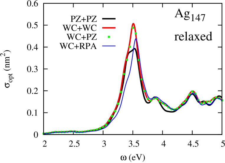
Figure 1: Absorption cross section of the icosahedral Ag₁₄₇ cluster computed with LDA and GGA functionals. The curves are labeled according to the xc potential (first label) and xc kernel (second label) used. The Perdew-Zunger (PZ) LDA functional and Wu-Cohen (WC) GGA functionals are compared. Blue solid line represent RPA $K_{\mathrm{xc}}=0$ starting from WC results. Relaxation of geometries was done with PZ or WC functionals.

With respect to electronic structure, it is well known from the literature that LDA and GGA predict a too low onset of the $d$-bands in the solid and this reduces the intensity of the low-frequency plasmonic resonance produced mainly by the $s$-electrons [79]. This deficiency of LDA and GGA can be corrected by using so-called long-range-corrected (LRC) xc functionals which contain a portion of Fock exchange [41, 37, 74], the van-Leeuwen-Baerends explicit ansatz with the correct asymptotic behavior [80], or orbital-dependent functionals [81, 11]. Unfortunately, these functionals are not available within the publicly-available version of the SIESTA package [44]. Moreover, the LRC functionals referenced above give rise to a non-local two-point TDDFT kernel, which is either not known or computationally too expensive to treat the large systems addressed here. From this point of view, the Sternheimer approach and wave-packet propagation approach have an advantage versus iterative TDDFT: former approaches only need the xc potential, and do not involve the TDDFT kernel. Fortunately, local and semi-local functionals correctly capture trends of the plasmonic response in nano-particles as was well documented in the past [73], and are still widely used [82].

For these reasons, we have the WC functional for both, the DFT and TDDFT steps of our calculation. In order to assess the effect of the xc functional, we compare the LDA and GGA spectra and also analyse the contributions from $d$-electrons to the total absorption cross section (in section 2.7 and 3.5). In the figure 1 we compare the optical absorption cross-sections computed with LDA and GGA functionals for the Ag₁₄₇ icosahedral cluster. The geometries of the cluster were relaxed with Perdew-Zunger (PZ) LDA or WC functionals, although the relaxations themselves did not affect the spectra significantly. We can immediately confirm that GGA increases the intensity of the plasmon peak as compared with LDA. However, it does not significantly shift the resonant frequencies (3.5 eV LDA, 3.54 GGA). Moreover, it is interesting to note that the effect of the gradient corrections in the kernel $K_{\mathrm{xc}}$ is marginal. Namely, in figure 1 we can hardly distinguish the spectra in which the GGA kernel is substituted by the LDA kernel and the other computational parameters are kept the same (WC+WC versus WC+PZ curves). As expected, however, the effect of Hartree kernel is crucial. The non-interacting response (not shown in the plots) is dominated at low energies by a peak at approximately 1 eV, way too low as compared to experiment. Therefore, we see a minor influence of xc kernel on the optical response of our Ag nanoparticles. It is important to note, however, that the improved approximation to the quasi-particle spectrum provided by the KS eigenvalues computed with the GGA functional is reflected in an improved description of the optical properties. This is an important information from a methodological point of view because the calculation of real-space integrals of the xc kernel is much more time consuming (two orders of magnitude) than the calculation of the Hartree kernel. The Hartree kernel is calculated with the help of fast Bessel transforms [83, 84] and the multipole expansions [85, 42]. Moreover, the GGA xc kernel is way more cumbersome than the LDA kernel (see B) and for many of the most sophisticated functionals the explicit expressions of the kernel are still lacking. The analysis presented above with respect to the influence of the xc kernel (RPA versus GGA) is consistent to the previously published for smaller clusters [39].

2.6 Choice of atomic orbital basis set

The choice of the atomic-orbital basis set determines the quality of LCAO calculations to a large extend. The numerical orbitals used in the SIESTA package are capable to approach the results of plane-wave calculations for bulk systems [86, 87], at least for ground state properties and the description of the low lying unoccupied states. At the same time, it was found that semi-infinite systems (surface properties) need special care when being described using confined NAO [88]. Namely, it was found that adding a single layer of floating orbitals can considerably improve the surface properties with only a small impact on the computational performance. Because the surface-to-volume ratio of our target clusters is rather large [1], we assess the quality of the default SIESTA basis set by augmenting it with an extra layer of floating orbitals.

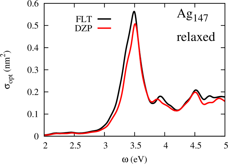
Figure 2: Absorption cross section of the icosahedral Ag₁₄₇ cluster computed with a DZP basis set and with a DZP basis augmented with an extra layer of floating orbitals (FLT). Relaxations have been done for all atoms except “ghost atoms” that carry floating orbitals.

In figure 2, we plot the absorption spectra of the Ag₁₄₇ cluster computed with a double-zeta polarized (DZP) basis (EnergyCutoff=50 meV) and with the same DZP basis augmented with an extra layer of $s$- and $p$- floating orbitals. The floating orbitals are placed at the positions of the next (fifth) Mackay layer (geometry of clusters is discussed below in section 3) and are excluded from the relaxation procedure. The WC functional was used in both calculations. One can see on the figure that the extra layer of floating orbitals slightly redshifts the frequency of main plasmon resonance (by 0.02 eV) and increases the absorption cross section around the resonance. A direct analysis of the absorption cross section in terms of the different cluster layers (see section 2.7) shows that the enhancement is due to the extra layer of “ghost atoms” which carry the floating orbitals (see subsections 2.7 and 3.5) and that the main contribution to the cross section is still due to the outer layer of real atoms. At the same time, the layer of floating orbitals does not affect the computation cost dramatically because it does not unnecessarily decrease the sparsity of the matrices involved in the calculation, which is the case when spatially extended diffuse orbitals are added to the basis set.

2.7 Analysis of the interacting density change.

Here we focus on the analysis of the interacting polarizability in terms of the spatial distribution of atoms and in terms of the non-interacting electron-hole pairs. Other type of analysis are too technical for a general presentation and we reserved them for A.

2.7.1 Contribution of different atoms to the polarizability.

In our framework, the interacting polarizability $\alpha(\omega)$ is given by

$$\alpha(\omega)=d^{\mu}\delta n_{\mu}(\omega),\ d^{\mu}=\int F^{\mu}(\bm{r})\bm{r}dr,$$ (23)

where we drop all Cartesian indices for the sake of clarity. The index $\mu$ runs over all product functions $F^{\mu}(\bm{r})$, which are centered on real and ghost atoms. The sum over product functions can be split into sub-sums according to a given criterion. For instance, we can split the sum over the product indices into sub-sums over atomic layers in the cluster $L$: $\alpha(\omega)=\sum_{L}\alpha_{L}(\omega)$ with a partial polarizability $\alpha_{L}(\omega)$ given by

$$\alpha_{L}(\omega)=d^{\mu}P_{\mu}^{\nu}(L)\delta n_{\nu}(\omega).$$ (24)

Here a padding operator $P_{\mu}^{\nu}(L)$ is introduced. The padding operator is a diagonal matrix whose elements are equal to one $P_{\mu}^{\mu}(L)=1$ if the product index $\mu$ belongs to an atom in the layer $L$ and zero otherwise.

2.7.2 Electron-hole expansion of the interacting induced density.

The analysis presented above for the interacting polarizability can be completed using an expansion of the interacting density change $\delta n(\bm{r},\omega)$ in terms of electron-hole pairs

$$\delta n(\bm{r},\omega)=\sum_{ij}\delta n_{ij}(\omega)\Psi^{*}_{i}(\bm{r})\Psi_{j}(\bm{r}),$$ (25)

where $\Psi_{j}(\bm{r})$ are KS eigenstates.

This kind of expansions are naturally arising in the Casida formulation of TDDFT [89] and this is perhaps at the root of the popularity of Casida’s formulation, because the electron-hole expansion (25) allows classifying a given excitation in terms of the character of the non-interacting transitions contributing to it, as was recently elaborated with an alternative method [90].

Obtaining the expansion (25) is relatively straightforward in the iterative formulation of TDDFT presented above. The interacting density change $\delta n(\bm{r},\omega)$ is given by (compare with equation (1))

$$\delta n(\bm{r},\omega)=\int\chi_{0}(\bm{r},\bm{r}^{\prime},\omega)\delta V_{\mathrm{eff}}(\bm{r}^{\prime},\omega)dr^{\prime},$$ (26)

where $\delta V_{\mathrm{eff}}(\bm{r},\omega)$ is an effective (screened) perturbation. Using sum-over-states representation (2) of the non-interacting density response function we can immediately see the electron-hole expansion coefficients $\delta n_{ij}(\omega)$

$$\delta n_{ij}(\omega)=\frac{f_{i}-f_{j}}{\omega-(E_{j}-E_{i})+\mathrm{i}\varepsilon}\int\Psi^{*}_{j}(\bm{r}^{\prime})\Psi_{i}(\bm{r}^{\prime})\delta V_{\mathrm{eff}}(\bm{r}^{\prime},\omega)dr^{\prime}.$$ (27)

Now it remains only to derive an equation for the effective perturbation $\delta V_{\mathrm{eff}}(\bm{r},\omega)$. Using the Petersilka-Gossmann-Gross equation (3) and the two alternative expressions (26) and (1) for the interacting density change, it is straightforward to derive an equation for the effective perturbation

$$\left[\delta(\bm{r}-\bm{r}^{\prime})-K(\bm{r},\bm{r}^{\prime\prime})\chi_{0}(\bm{r}^{\prime\prime},\bm{r}^{\prime},\omega)\right]\delta V_{\mathrm{eff}}(\bm{r}^{\prime},\omega)=\delta V_{\mathrm{ext}}(\bm{r},\omega).$$ (28)

In terms of product basis (8) and for optical absorption $\delta V_{\mathrm{ext}}(\bm{r},\omega)\equiv\bm{r}$, the latter equation transforms into a linear algebraic equation

$$\left[\delta-K\chi_{0}(\omega)\right]\delta V_{\mathrm{eff}}(\omega)=d,$$ (29)

where we dropped Cartesian indices and product indices for clarity. This equation can be solved iteratively with a generalized minimal residue solver [70]. Using the product basis again in equation (27) we get

$$\delta n_{ij}(\omega)=\frac{(f_{i}-f_{j})(X^{j}_{a}V^{ab}_{\mu}X^{i}_{b})}{\omega-(E_{j}-E_{i})+\mathrm{i}\varepsilon}\delta V^{\mu}_{\mathrm{eff}}(\omega).$$ (30)

Having the density change in terms of electron-hole pairs (30) we can define a transition-resolved optical polarizability

$$\alpha_{ij}(\omega)=\delta n_{ij}(\omega)\int\Psi^{*}_{j}(\bm{r})\bm{r}\Psi_{i}(\bm{r})dr$$ (31)

and thus assess the contribution of each non-interacting pair of states to the true, interacting polarizability. Moreover, it is now possible to answer questions related to the symmetry of the charge density with a strongest contribution at a given frequency [38] and perform other types of analysis analogous to the crystal orbital overlap and Hamiltonian populations analysis of density matrix [54]. Here, we will focus on the analysis of the polarizability in terms of the dominant atomic angular-momentum contributions in the initial state. For this, we will explicitly separate the occupied and virtual states and look for the electron-hole expansion in the form

$$\delta n(\bm{r},\omega)=\sum_{i\in\mathrm{occ},j\in\mathrm{unocc}}\delta n_{ij}(\omega)\Psi^{*}_{j}(\bm{r})\Psi_{i}(\bm{r}),$$ (32)

where the expansion coefficients $\delta n_{ij}(\omega)$ read

$$\delta n_{ij}(\omega)=\left(\frac{(f_{i}-f_{j})(X^{i}_{a}V^{ab}_{\mu}X^{j}_{b})}{\omega-(E_{j}-E_{i})+\mathrm{i}\varepsilon}-\frac{(f_{i}-f_{j})(X^{i}_{a}V^{ab}_{\mu}X^{j}_{b})}{\omega+(E_{j}-E_{i})+\mathrm{i}\varepsilon}\right)\delta V^{\mu}_{0}(\omega).$$ (33)

Now we can define a polarizability resolved in the angular momentum $l$ of the occupied states

$$\alpha_{l}(\omega)=\sum_{i\in\mathrm{occ},j\in\mathrm{unocc}}\delta n_{ij}(\omega)X^{j}_{a}d^{ab}\delta_{l_{a},l}X^{i}_{a}.$$ (34)

Obviously, the partial polarizability $\alpha_{l}(\omega)$ add up to the total interacting polarizability $\alpha(\omega)=\sum_{l}\alpha_{l}(\omega)$ and each of the partial polarizabilities gives an idea of the contribution of a given symmetry in the occupied states to the total polarizability. The result of this analysis for silver clusters is presented below in subsection 3.5.

3 Results

In this work, we focus our attention on silver clusters and shells, which are well known plasmonic systems. We will address the dependence of the plasmonic resonances on the system size, the thickness of the shells and the details of the cluster geometry (relaxation method).

3.1 Calculation parameters

Clusters of icosahedral shapes were constructed using the atomic simulation environment [91] according to a Mackay motif [92]. The initial atomic positions were obtained using a 4.0 Å lattice constant that is close to the GGA-relaxed geometry and is smaller than experimental lattice constant for bulk Ag (4.09 Å). The “ideal” geometries were relaxed by minimizing the forces acting on atoms below 0.02 eV/Å using the GGA functional after Wu and Cohen [78, 72], as we discussed in subsection 2.5. Otherwise said, we used similar parameters in all calculations. The spatial extension of orbitals was set in a default procedure by an EnergyShift parameter of 50 meV and a double-zeta polarized (DZP) set of atomic orbitals was used. The real-space mesh has been set via a Meshcutoff=150 Ry. Only valence electrons (5s¹4d¹⁰) are represented in the atomic orbitals set, which give rise to 15 atomic orbitals per atom in the DZP basis set. Moreover, we added a layer of floating orbitals (see subsection 2.6) in the cluster calculations and two layers of floating orbitals—inner and outer—in the case of shell geometries. Coordinates of these “ghost atoms” were kept fixed during relaxations.

The core electrons are removed by using the pseudo-potential (PP) of Troullier-Martins type. The PPs were generated with the ATOM program, part of the SIESTA distribution. The parameters for PP generation were taken from the SIESTA database [93] except for the use of Wu and Cohen functional. It is interesting to note that the optimized PP described in Ref. [94], which is supposed to provide a band structure in better agreement with all-electron calculations, failed to satisfactorily describe the optical absorption cross section. Indeed, the description is severely worsen and the main plasmonic resonance disappears.

3.2 Relaxed geometries

A set of representative clusters and cluster shells are shown in figure 3. We characterize icosahedral clusters by the number of atom layers present in the cluster and refer to this number as size of the cluster. Cluster shells are constructed starting from a cluster and keeping only several outer atomic layers—similar to the approach adopted by other groups [28, 29]. The number of atoms in a particular layer $l>1$ is given by $N(l)=10l^{2}-20l+12$. The first “layer” is composed of one atom. For example, the largest cluster we considered is composed of six atom layers (denoted S6L6) which makes in total 1+12+42+92+162+252=561 atoms, while the icosahedral shell S7L4 will contain 92+162+252+362=868 atoms.

As already mentioned, we optimize the geometries of the clusters and shells in order to account for rearrangement effects caused by surface stresses. Geometrical relaxations were done by minimizing the total forces as implemented in SIESTA. The DFT relaxation only slightly compressed the ideal Mackay structures. For instance, the distance between extreme atoms 1 and 2 marked in figure 3 for the S4L4 cluster is 14.76 and 14.52 Å for the ideal geometry (in which the experimental lattice constant 4.09 Å is used) and the Wu and Cohen geometry, respectively.

The surface stress also tends to distort (round up) ideal geometries. For instance, the distance between atoms 1 and 2 in the S5L5 cluster is slightly different than the distance between extreme atoms 3 and 4 (see figure 3). The distance $d_{12}$ is 19.68 and 19.40 Å for the ideal and the GGA geometries respectively, while the distance $d_{34}$ is 19.23 Å for the GGA geometry.

Both geometry distortions (overall compression and rounding) are present in the silver shells. For instance, the GGA-relaxed length $d_{12}$ in the S4L1 shell is 13.79 Å. Distances $d_{12}$ and $d_{34}$ in S5L1 shell are 18.18 and 18.14 Å, respectively. Notice that these distances are smaller than those in the corresponding compact structures, indicating a larger compression in the case of mono-layered shells.

Summarizing the outcome of GGA geometric relaxations, we note that relaxation leads to minor geometrical distortions of the ideal icosahedral clusters. However, it leads to relatively large compressions for thin silver shells. For instance, if we characterize the compression with an averaged bond length in the edge of clusters (chosen as a simple measure and representative for the other nearest neighbor distances in the cluster), then the mono-layered shells have that bond length compressed by 6% (2.80 Å) as compared to the average bond length in the compact clusters (2.97 Å). The cluster averaged bond length is also compressed by 2.4% as compared to the ideal bond length (3.04 Å) calculated with the experimental lattice constant of bulk silver.

	S3	S4	S5
L1
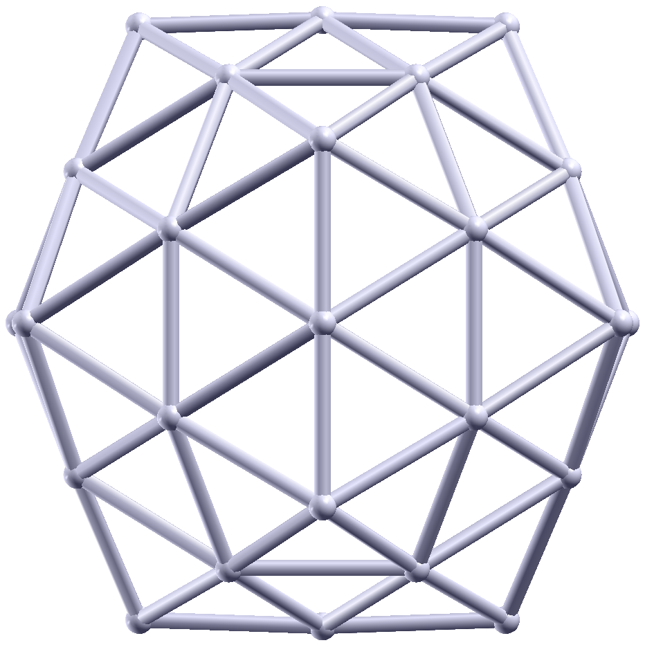
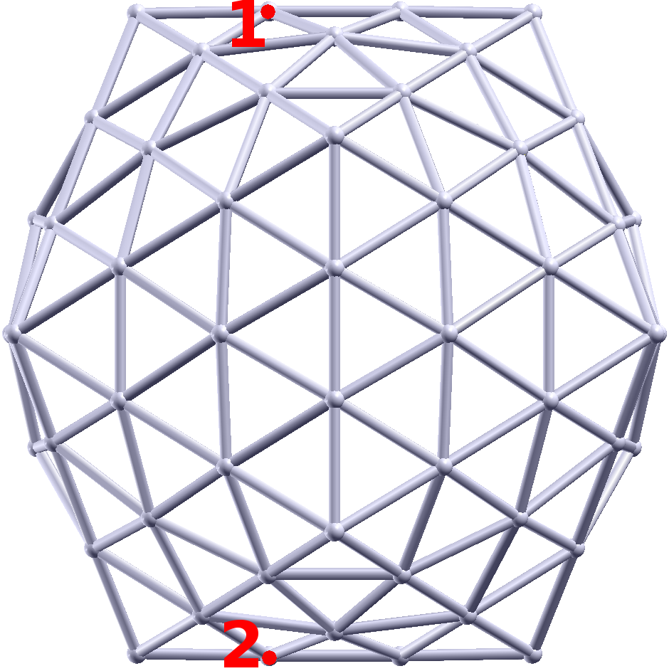
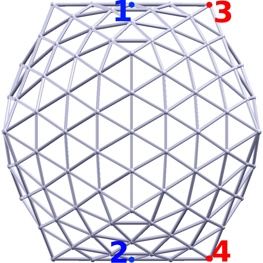
L2

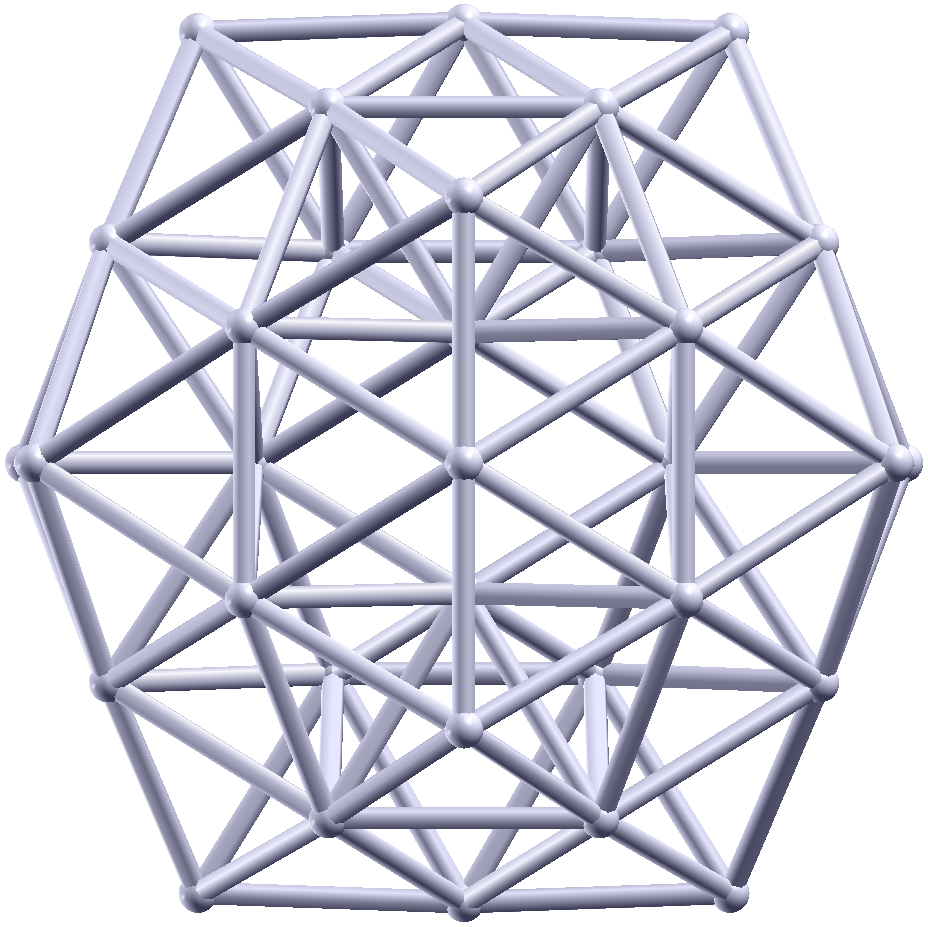
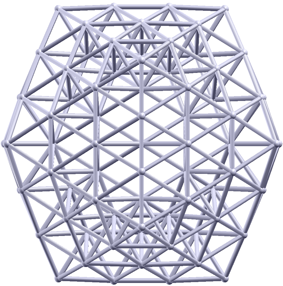
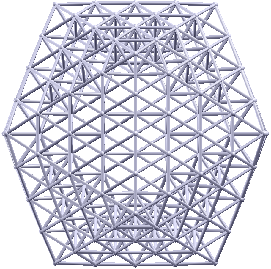
Figure 3: Relaxed geometries of icosahedral silver clusters. Labels S3, S4, S5 refer to the number of atom layers present in the clusters. Labels L1, L2 refer to the number of layers that are kept in a given cluster shell. The structures in the lowest row represent compact clusters. Atoms whose relative distances are discussed in text are marked by colored numbers.

3.3 Optical absorption of Ag_N icosahedral clusters

Qualitatively, one expects that the plasmon resonance is affected by the size and morphology of the clusters. In order to assess the magnitude of this dependence, we performed TDDFT calculations of the absorption spectra for compact clusters and shells. The smallest cluster is composed by two layers (Ag₁₃), while the largest cluster consists of six layers (Ag₅₆₁). In order to assess the effect of removing internal atoms, we also performed calculations of hollow structures, keeping up to four outer atomic layers in a given system.

In order to expand the response and induced density we have chosen an atom-centered product basis as described in section 2 with 77 functions per atom. The dominant product basis [64, 65, 42] is used as an intermediate basis in the application of the non-interacting response, as explained above. Depending on the system, the size of the dominant product basis is 2.4–4.1 times larger than that of the atom-centered product basis. The generation of the product basis $A^{\mu}(\bm{r})$ and the calculation of interaction matrices $K^{\mu\nu}$ takes a relatively small amount of time. For instance, in the case of our largest Ag₅₆₁ cluster, a 12 core Intel machine spends (approximately) 45, 1 and 260 minutes, respectively for the basis set generation, and the calculations of Hartree- and GGA- kernels. The iterative procedure normally takes most of the walltime. We decided to compute the absorption spectra in a range 0–10 eV, with a frequency step $\Delta\omega=0.05$ eV, and a broadening constant $\varepsilon=0.08$ eV (i.e. full-width at half maximum is 0.16 eV). This consistent choice of frequency step and broadening ensures that we do not “overlook” any feature present in the computed data and also produces data that can be well interpolated.

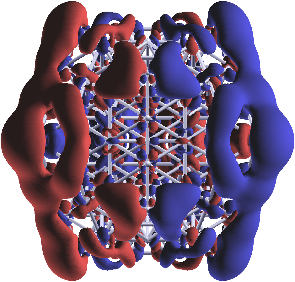
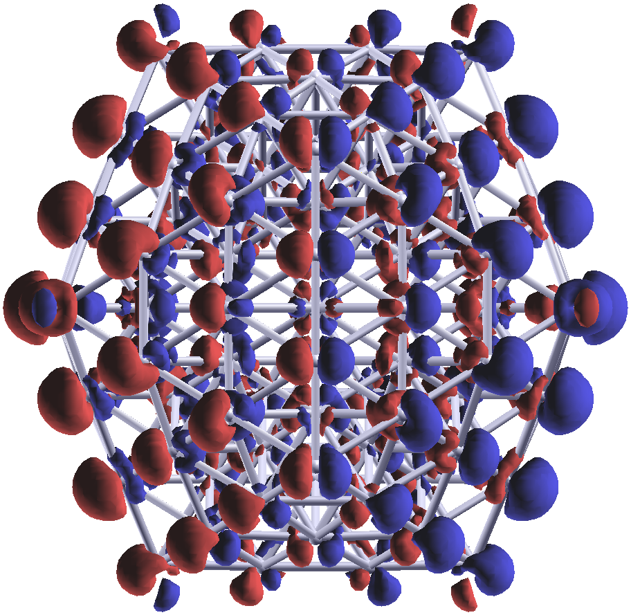
a)	b)	c)

Figure 4: The absorption cross sections of silver clusters of icosahedral shape are shown on panel a). One can recognize resonances around 3–4 eV (sharp) and 6–7 eV (very broad). Panel b) and c) show the isosurfaces of density change $\mathrm{Re}(\delta n(\bm{r},\omega))$ for the Ag₁₄₇ cluster at the frequencies 3.4 and 6.6 eV, respectively.

We focus our attention on the optical absorption properties of compact icosahedral geometries and then will move to a comparison with silver shells in the next subsection 3.4. Photo-absorption cross sections are shown in the figure 4 (a). The cross section possesses two maxima: a sharp peak at 3–4 eV and a broad maximum around 6–7 eV. The frequencies of the resonances decrease for larger clusters. For instance, the two largest clusters Ag₃₀₉ and Ag₅₆₁ have the absorption maxima at 3.37 and 3.25 eV in the low-frequency band and at 6.7 and 6.2 eV in the high-frequency band, respectively. Panels b) and c) in figure 4 show the induced density change (solution of equation (21)) in the Ag₁₄₇ cluster at the maxima of the low-frequency and high-frequency bands, respectively. The direction of external field is set along x axis, i.e. collinear with the plot plane and horizontal. The isosurfaces of the real part of $\delta n(\bm{r},\omega)$ were plotted for a 10% of the corresponding maximal value. One can see that the low-frequency resonance is caused by an oscillation of charge with pronounced dipole character, while the high-frequency band is supported by more localized, homogeneously-spread oscillations. The lower energy resonance obviously corresponds to the dipole Mie plasmon of the particle. From a quantum mechanical point of view, both bands consist of many nearly-degenerate transitions. The number of the transitions makes it impractical to analyse each of them in detail. However, one can provide some analysis of the electronic transitions and atom-layer contributions as demonstrated below in subsection 3.5.

3.4 Optical absorption of silver shells

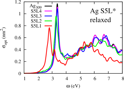
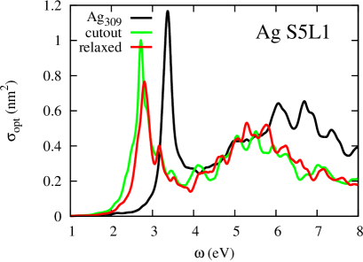
a)	b)
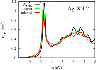
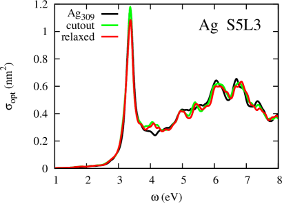
c)	d)

Figure 5: The absorption cross sections of icosahedral silver shells constructed from the Ag₃₀₉ cluster. On panel a) the cross section of the Ag₃₀₉ cluster is shown together with the cross sections of the one- to four-layered shells. On panel b) the optical absorption cross sections of “cutout” and relaxed single-layered silver shells are compared (see text for details). Panels c) and d) show the cross sections of cutout and relaxed two- and three-layered silver shells, respectively.

Silver shells can be constructed from the initial geometry of the corresponding cluster in several ways. We suggest two useful ways to construct the silver shells. In the first way, we simply delete atoms of several inner atomic layers from the compact cluster that was previously relaxed within DFT. In the second way, we additionally relax the positions of the atoms remaining in the shell. The former way is less computationally demanding and also is eventually more useful to approximate the response of the whole cluster by the response of its outer shell. The latter way should give results that are closer to the corresponding experimental values for shells. In figure 5, we analyse the optical absorption cross section of the Ag₃₀₉ cluster and of silver shells derived from that cluster. In panel a) we show the cross sections of the relaxed shells. It is worth noting that a single-layered shell (S5L1, Ag₁₆₂) exhibits a low-frequency resonance at 2.8 eV which must be compared to the 3.37 eV in the case of the Ag₃₀₉ cluster. If we leave two atomic layers as in the silver shell S5L2 (Ag₂₅₄), then the low-frequency band shifts back (3.28 eV) almost to the frequency of the full cluster. The broad high-frequency resonance of the silver shells qualitatively follows the same behavior. Namely, the maximum frequency of the single-layered shell is red shifted to 5.8 eV that must be compared to 6.7 eV in the case of Ag₃₀₉ cluster. However, already a two-layered shell almost recovers (6.5 eV) the position of the maximum of the high-frequency band for the compact cluster. The optical cross sections of the three- and four-layered shells approach that of the cluster steadily.

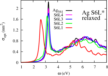
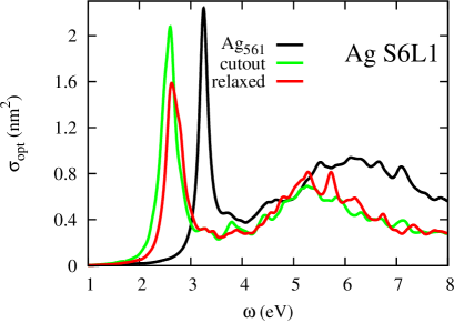
a)	b)
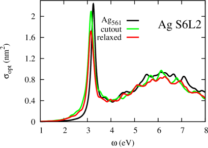
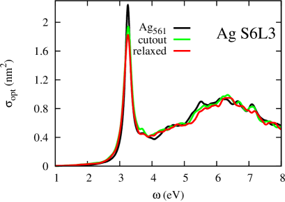
c)	d)

Figure 6: The absorption cross sections of icosahedral silver shells constructed from the Ag₅₆₁ cluster. On panel a) the cross section of the Ag₅₆₁ cluster is shown together with the cross sections of the one- to three-layered shells. On panel b) the optical absorption cross sections of cutout and relaxed single-layered silver shells are compared. Panels c) and d) show the cross sections of cutout and relaxed two- and three-layered silver shells, respectively.

The effect of geometry relaxation in the silver shells is also quantified in figure 5. The panels b), c) and d) show the optical absorption cross sections of the one-, two- and three-layered silver shells, the geometry of which was either “cutout” from the geometry of the Ag₃₀₉ cluster or optimized (relaxed). The comparison shows that the effect of geometry relaxations is the much larger for the single-layered shell than for the other shells. The relaxation leads to slight blue shift of both bands. This is due to the additional compression of the structure when relaxed. Moreover, relaxations result in a broadening of the low-frequency resonance and in an relative increase of the cross section in the high-frequency band in the single-layered shell (panel a). Panels c) and d) show that the effect of geometry relaxation is less important for thicker shells. Cutout structures, created by simply removing the internal layers of atoms, give results very similar to those of the relaxed shells.

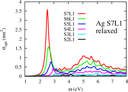
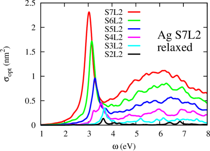
a)	b)
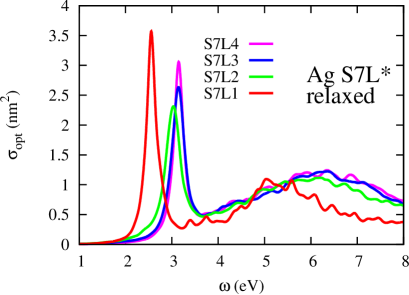
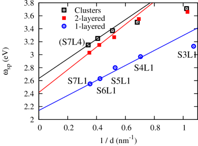
c)	d)

Figure 7: The absorption cross sections of the single- (panel a) and double-layered (panel b) icosahedral silver shells. On panel c) the absorption cross sections of shells of size 7 are compared. The plasmon frequency versus size of the clusters and shells on panel d). Lines on panel d) are drawn through the points corresponding to largest structures (S6 and S7).

In figure 6 we show the optical absorption cross sections of the 6-layered icosahedral silver cluster and shells constructed from that cluster. The cross sections show qualitatively the same behavior as those of the 5-layered cluster and shells (see figure 6 panels a), b), c) and d)). Namely, the cutout and relaxed one-layered shells S6L1 have the red-shifted low-frequency resonance at 2.6 and 2.62 eV, correspondingly, while the cross sections of two- and three-layered shells are much closer to that of the full cluster (3.25 eV). However, the low-frequency band of the two-layered shells S6L2 differs more from that of the compact cluster (3.15 eV for cutout and relaxed geometries). It is also interesting to note that geometry relaxations of the one- and two-layered shells lead to a small blue shift relatively to the unrelaxed calculations. In the case of three-layered shell S6L3, however, the geometry relaxations lead to a slight red shift (3.25 eV) of the low-frequency maximum in comparison to the “cutout” geometry (3.26 eV).

In figure 7 we collected the optical absorption of all single- (panel a) and double-layered (panel b) shells computed in this work. The cross section of the shells is qualitatively similar to the cross section of the clusters: there are low-frequency sharp and high-frequency broad resonances, the maxima of these resonances steadily decreases with increasing the cluster size. The ratio of low-frequency to high-frequency intensities is nearly the same in compact structures and shells of sizes up to 6, while for the largest single-layered shell S7L1 the relative intensity of the low-frequency peak increases. The low-frequency peak in the absorption cross section of the S7L1 shell is more intense than for the S7L2 shell (figure 7, panel c), in contrast to what is observed in smaller shells (figures 5 and 6). The absorption cross section of the thicker largest shells (S7L3 and S7L4) should approach the response of the compact cluster of the same size. Unfortunately, we could not compute the absorption of the cluster Ag₉₄₃, because of the large memory requirements, but we can be reasonably sure that the thickest shell S7L4 represents well the absorption of the compact cluster of size 7. The frequency of maximal absorption shows an approximately linear dependency on the inverse diameter of clusters as shown on panel d) both for clusters and shells. The effective diameter of the clusters and shells has been computed from the spatial cross-section of the cluster, while the diameter of the cluster is defined as the diameter of a circle with the same area. The data shown in figure 7 (d) indicates small discrepancies from the linear trend both for compact geometries and double-layered shells for smaller clusters, while in the case of single-layered shells such discrepancy is visible only for smallest shell.

3.5 Analysis of the optical absorption

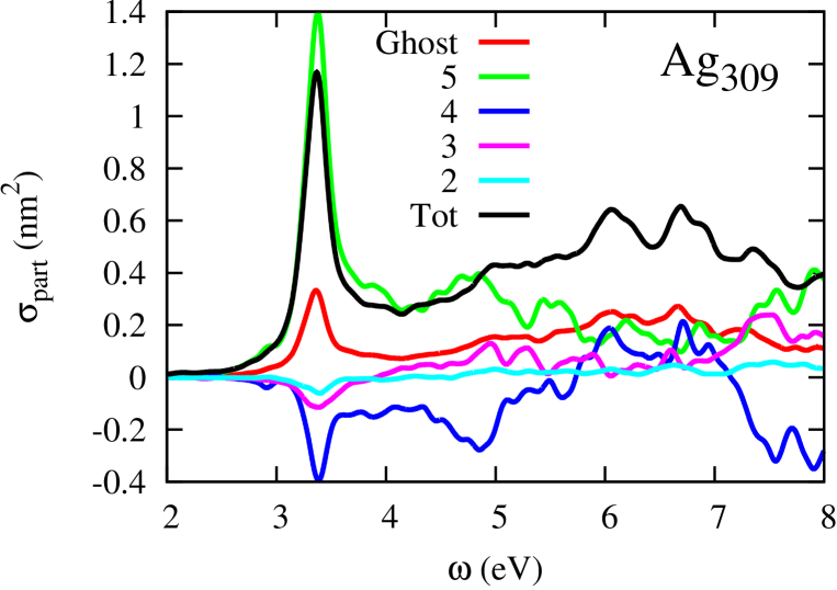
Figure 8: Contribution of the different atom layers to the absorption cross section of the Ag₃₀₉ cluster (S5L5).

In figure 8 we show the analysis of the atom-layer contributions to the optical absorption cross section according to the method presented above in section 2.7. The partial cross sections corresponding to different atom-layer polarizabilities (24) are plotted together with the total absorption cross section. The outer layer (5-th layer, 162 atoms) gives rise to the largest partial cross section that is even larger than the total cross section at resonance. The 6-th layer of “ghost atoms” is contributing constructively in the whole frequency range and with a rather large magnitude that is approximately equal to that of the second inner layer (4-th layer) of “true” atoms. The inner atomic layers give rise to negative partial cross sections at least in some frequency ranges. At the main resonance 3.37 eV, all inner layers contribute destructively. The second outer layer (4-th layer, 92 atoms) gives rise to a negative partial cross section in most of the frequency range considered. The contribution of the first “layer” that is composed of one atom is much lower than that of the next layer (2-nd layer, 12 atoms) and is not shown.

The interpretation of these results in the low-frequency range is quite clear. As expected from the plot in figure 4 (b), and consistent with the Mie plasmon character of the resonance, the main contribution is coming from the surface layer. For this mode, it is critical to describe accurately the polarization of the surface, which explains the large contribution of the layer of “ghost atoms” above cluster surface. Those basis orbitals control the extension of the electronic states towards vacuum and, therefore, are instrumental to correctly account for the polarizability of the surface. The change of signs is related to the relative phases of the different contributions, reflecting to some extent the global nodal structure of the contributing electronic states.

At higher energies, the smaller dielectric function of bulk silver makes the charge screening less efficient, the modes loose their predominant surface character, and the contributions of different layers become more similar in intensity.

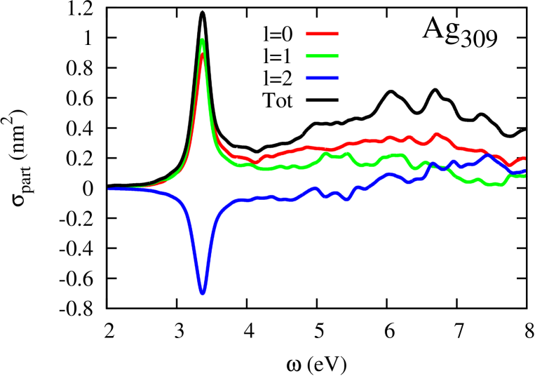
Figure 9: Analysis of the different angular momenta of the basis orbitals involved in the description of the occupied states contributing to the absorption cross section of the Ag₃₀₉ (S5L5) cluster as function of frequency.

In figure 9 the partial cross sections (corresponding to the partial polarizabilities (34)) for atomic orbitals of different symmetry expanding the occupied states are shown for Ag₃₀₉ cluster. We see that, on the absolute scale, the contribution of each angular momentum channel is important even at low frequencies. However, there is a striking difference between $s$, $p$ and $d$ contributions to the absorption cross section. Namely, the $s$- and $p$- channels contribute constructively to the absorption cross section, while $d$ channel contributes destructively in the low frequency range (3–4 eV) and only starts to contribute constructively at high frequencies, starting approximately at 5.5 eV. This conclusion is similar to that presented in a previous LDA study for smaller silver clusters [73]. This theoretical analysis supports the view of the low-frequency excitation as produced by $5s$ electrons [95] only partially. This is because the occupied states are $sp$-hybridized close to Fermi energy and also there is a non-negligible contribution of $s$-symmetrical density at higher frequencies (6–7 eV). From the other side, the strong over-screening of the $s$ plasmon due to $sp$-$d$ interband transitions has been discussed at length in the literature [80, 74]. The comparison of our data with those in Refs. [74, 11] suggests that GGA could underestimate the intensity of $s$ plasmon by a factor about $1.5$.

In order to comprehend better the outcome of ab-initio modeling we compare our results with the available relevant literature in the following section.

4 Discussion

Because the clusters that we have considered are rather large, we expect that their properties will approach the properties of classical Mie spheres [7, 73] to the extent that the non-sphericity of icosahedra and charge spillage effects allow. The classical absorption cross section in the electrostatic limit depends on the dielectric function of the material $\epsilon(\omega)$ and the dielectric function of the embedding medium $\epsilon_{m}(\omega)$ [96, 7]

$$\sigma(\omega)\sim\omega\,\mathrm{Im}\frac{\epsilon(\omega)-\epsilon_{m}(\omega)}{\epsilon(\omega)+2\epsilon_{m}(\omega)}.$$ (35)

If we plot the cross section (35) with the experimentally determined dielectric function of silver [97, 98], then we will get a sharp low-frequency resonance and a less intense and broad high-frequency resonance as it is shown in the figure 10 panel a). The position of the resonances slightly varies with the set of experimental data used. The more recent experiment [98] gives resonance maxima at 3.53 and 6.8 eV, while the older and widely cited experimental results [97] give them at 3.47 and 6.1 eV, correspondingly. The response in the low-frequency part of the spectra is detailed in the panel b) of the figure 10.

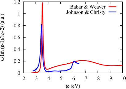
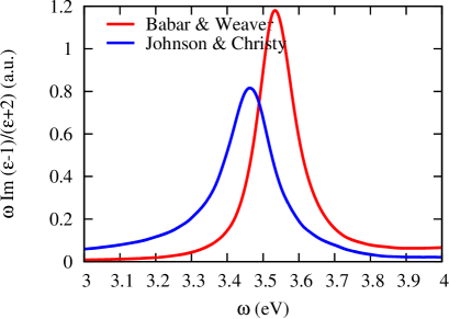
a)	b)

Figure 10: The absorption cross section in a classical quasi-static limit for a silver sphere in vacuum. Experimentally-determined dielectric function of silver is used.

Comparing the quasi-static absorption cross section (35) with our results, we see similarities and discrepancies. First of all, the resonance frequencies from Mie theory do not depend on the size of the object, but only on its shape. Classical estimations of the shape influence [11] lead to a conclusion that icosahedral particles have to resonate at 2.9% lower frequencies than perfectly spherical clusters.

TDDFT accounts for charge spillage at surfaces (i.e., the fact that surfaces are not perfectly sharp, as assumed usually in classical electrodynamics) which leads to a divergence of the plasmon frequency $\omega_{\mathrm{sp}}$ from a linear dependence $\omega_{\mathrm{sp}}=kd^{-1}+b$ with respect to the inverse diameter for small clusters (see figure 7 d). Measurements of the optical absorption of small silver clusters support this conclusion at least qualitatively [99, 100, 24, 101]. The divergence from the linear dependence in the experimental data must be due to charge spillage, because the other effect that leads to red shifts – higher multipole contributions to the electron-photon coupling – does affect only relatively large clusters of diameters 50 nm and larger [102].

In the case of the smallest cluster presented here Ag₁₃, there are experimental data [103, 104] for argon embedded clusters that show a maximum absorption strength at 3.4-3.5 eV while we get 3.63 eV. Because the effect of argon embedding can lead to red shifts as large as 0.3–0.5 eV [105, 101], we estimate that TDDFT with GGA functional might be delivering red-shifted frequencies by about 0.2 eV. In the case of larger clusters, we can compare with experimental data [24] measured on free silver clusters. For instance, for a cluster diameter of 1.2 nm, which corresponds approximately to our Ag₅₅ cluster, the experimental peak position is 3.51 eV, while we get 3.7 eV. For a cluster diameter of 2.2 nm, which corresponds to our Ag₃₀₉ cluster, the experimental peak position is 3.47, while we get 3.37 eV. For a cluster diameter of 2.8 nm, which corresponds to our Ag₅₆₁ cluster, the experimental peak position is 3.45, while we get 3.25 eV. These comparisons indicate that our calculations deviate by no more than 0.2 eV from experiment, presenting a somewhat stronger size dependency than observed experimentally. The computed plasmon frequencies are red-shifted for large clusters.

Besides experimental results, there are many calculations of silver optical absorption properties available in the literature. The first observation is that very little can be found on the broad resonance in the frequency range 5.5–7.5 eV, although this feature must be available in the calculations done with atomistic codes. This is probable due to little practical relevance of the frequency range and the much stronger low-frequency plasmonic response.

The position and strength of the low-frequency plasmonic peak depends on the used functional and the basis set: the agreement with experiment improves while using more sophisticated functionals and larger basis sets. For instance, the use of the simplest LDA functional results in a too low energy onset of the $d$-bands in the electronic structure, [79] which leads to a reduced strength of the low-frequency resonance and its red shift as compared to experiment and calculations based on Hedin’s $GW$ band structures [79]. In this paper, we showed that GGA functional by Wu and Cohen produces a strong low-frequency peak for icosahedral clusters. GGA functionals have been extensively used in the past for silver cluster, [104, 36] as well as the more sophisticated long-range-corrected functionals: van Leeuwen-Baerends (LB94) [106], Gritsenko-van Leeuwen-van Lenthe-Baerends (GLLB) [11] and long-range corrected PBE (LC-$\omega$PBE) [107, 108, 37].

Quantitatively assessing the position of the low-frequency resonance, we can compare our results with several theoretical calculations. For Ag₁₃ cluster, we can find the values (in eV) 3.5 (PBE) [104], 3.5 (LC-$\omega$PBE) [37], 3.2 (LDA) [38], 3.7 (LDA) [39] and 3.2 (PBE) [109], while we get the maximum at 3.63 eV. For Ag₅₅ icosahedral cluster, we can find values 3.5 (LDA) [39] and 4.2 (GLLB) [11] eV, while we get the maximum at 3.71 eV. For Ag₁₄₇ icosahedral cluster, we can find values 3.8 (GLLB) [11], 3.2 (PBE) [36], 4.5 (LB94) [106], while we get the maximum at 3.5 eV. For Ag₃₀₉ icosahedral cluster, we can find values 3.7 (GLLB) [11], 3.50 (polarizability interaction model) [110], while we get the maximum at 3.37 eV. Finally, for Ag₅₆₁ icosahedral cluster, there is a value 3.65 eV from [11], while we get 3.25 eV. Summarizing, we see that the deviations between our calculations and other calculations that utilize the LDA or GGA functionals do not exceed 0.2 eV and might be due to differences in the used basis sets or pseudo-potentials. The larger deviations of about 0.4 eV, we have with LRC functionals.

Hollow structures have been produced and characterized [111, 112, 113, 114, 115, 14]. Experimental evidence supports our finding that the hollow structures have lower frequencies of the main plasmonic resonance. However, the measurements were performed with relatively large and thick shells (at least one order of magnitude larger than those considered here) and a quantitative comparison of our results with experiments is hardly possible.

From the theoretical side, there are several estimations for hollow metallic particles available. Firstly, the solution of Maxwell equations in the quasi-static limit for a hollow spherical particle is known [96] and the effect of removing interior part of the sphere is a red shift of the plasmon frequency. As in the case of compact spheres, the resonance frequencies do not depend on the size of the system, but only on the ratio of the inner and outer radius of the sphere. Secondly, there are atomistic TDDFT calculations for icosahedral shells of up to size of 6 layers available [28, 29]. These calculations show red shifted plasmonic resonances for hollow clusters compared to the filled ones. Quantitatively comparing the position of the low-frequency resonance, we get a fair agreement. For instance, for Ag₉₂ (S4L1 shell) we can find 3.85 (LB94) [29] and 2.8 (PBE) [28] eV, while we get 2.97 eV. For Ag₁₂, Ag₄₂, Ag₁₆₂ and Ag₂₅₂ (S2L1, S3L1, S5L1 and S6L1 shells) we extract from [29] 4.0, 4.35, 3.5 and 3.2 eV, while we get 4.17, 3.13, 2.8 and 2.63 eV, respectively. The discrepancies are sizeable, but can be explained by the differences of the functional (LB94 versus WC) and the geometry relaxations (ideal symmetric with the nearest-neighbor distance fixed at a equilibrium bulk value 2.89 Å versus fully relaxed geometries with no symmetry imposed in our case). The effect of geometry relaxations is estimated in subsection 3.4: it has a minor importance compared to the influence of DFT functional and does blueshift the resonances of the ideal structures with respect to those of relaxed ones.

The response of other silver made structures with effectively reduced dimensionality: rods [116, 117, 36, 37] and plateletts [113, 118] also exhibit red shifted resonance frequencies of the plasmon excitations with respect to spherical or quasi-spherical clusters of similar sizes.

5 Conclusion

We studied the optical response of silver clusters of icosahedral symmetry and their hollow counterparts by means of quantum mechanical, atomistic methods (linear response TDDFT within LCAO). The applied iterative methods allowed for comparatively fast calculations (about 1 day of walltime) of compact clusters containing up to 561 atoms and hollow clusters of up to 868 atoms. We have found that the plasmonic resonance of silver clusters depends on the size and morphology of clusters. Namely, the frequency of maximal absorption of the icosahedral clusters that contain three and more atom layers is inversely proportional to the cluster diameter. Moreover, the single-layered shells show a sizeable red shift of the resonance frequencies, which quickly becomes negligible as the thickness of the shells increases. Both observations are compatible with experimental findings, previous calculations, and can be partially understood within classical electrodynamics. Furthermore, both observations are valid also for the high-frequency, interband plasmon which was not widely studied so far.

From a methodological point of view, we presented recent developments of our iterative technique including a realization of an atom-centered product basis and various analysis tools. The iterative method used here [42], particularly with the speedup allowed by the use of an atom-centered auxiliary basis to express the orbital products, is advantageous in many respects that are discussed in the paper. In particular, the frequency-range selectivity is useful in calculations of the Raman response, for which one needs the response in a very narrow spectral range. Moreover, the current implementation of the response times vector operation can be easily optimized to be less memory demanding. This optimization will allow to extend the number of treated atoms by an order of magnitude, and even further if full MPI parallelization is implemented.

Appendix A Dominant basis set symmetries contributing to the optical polarizability

The prior analysis in section 2.7 has been formulated for a simple, physically motivated splitting of the interacting polarizability in terms of angular momentum of the occupied states and in terms of the atomic contributions to the optical polarizability. In this section, we focus on a more technical analysis of the interacting polarizability in terms of the products of atomic-orbital functions, and in terms of the product basis functions contributing to the resulting induced screened density change in the cluster.

Similarly to the analysis tools considered in section 2.7, the total interacting polarizability can be split into sums with fixed angular momentum of the product functions $F^{\mu}(\bm{r})$. This is so because the product functions are constructed as a linear combination of the products of atomic orbitals separately for each possible angular momentum of the product [65] and, therefore, the product function $\mu$ carries a well-defined angular momentum $l_{\mu}$. We can write the polarizability as a sum over angular momenta of the product basis $\alpha(\omega)=\sum_{l}\alpha_{l}(\omega)$ with a product angular momentum resolved polarizability $\alpha_{l}(\omega)$ given by

$$\alpha_{l}(\omega)=d^{\mu}\delta_{l_{\mu},l}\delta n_{\mu}(\omega),$$ (36)

where the dipole moments $d^{\mu}$ refer to a global origin of the coordinate system. The dipole moments are defined for product functions $F^{\mu}(\bm{r})$ that are centered on atoms

$$\bm{d}^{\mu}=\int F^{\mu}(\bm{r}-\bm{R}_{\mu})\bm{r}d^{3}r=\int F^{\mu}(\bm{r})\bm{r}d^{3}r+\bm{R}_{\mu}\int F^{\mu}(\bm{r})d^{3}r.$$ (37)

The last equation makes it apparent that only angular momentum $l_{\mu}=0$ and $l_{\mu}=1$ can contribute to the dipole polarizability.

Yet another type of analysis involves the angular momentum symmetry of the atomic orbitals, the products of which expand the density change $\delta n(\omega,\bm{r})$. Namely, the product function $F^{\mu}(\bm{r})$ is expressed in terms of a linear combination of the products of atomic orbitals (9). Therefore, we can immediately write the interacting polarizability $\alpha(\omega)$ as a sum over atomic orbital angular momentum sub-sums $\alpha(\omega)=\sum_{l_{1},l_{2}}\alpha_{l_{1},l_{2}}(\omega)$ with the partial polarizability $\alpha_{l_{1},l_{2}}(\omega)$ given by

$$\alpha_{l_{1},l_{2}}(\omega)=\delta_{l_{a},l_{1}}d^{ab}\delta_{l_{b},l_{2}}\Lambda_{ab}^{\mu}\delta n_{\mu}(\omega).$$ (38)

Here the dipole matrix elements between atomic orbitals is used $d^{ab}=\int f^{a}(\bm{r}-\bm{R}_{a})\bm{r}f^{b}(\bm{r}-\bm{R}_{b})dr$. Thus, recalling that the atom-centered functions are constructed from local on-site products, we see that the total polarizability can be expressed in terms of the on-site atomic orbitals. From the one side, this reveals a certain arbitrarity of the proposed separation, but from the other side, it might be useful for developing simplified models. Because the global origin and the atom centers do not generally coincide, there are no dipole selection rules in the matrix-elements $d^{ab}$. Namely, analogously to the case, of dipole moments (37), the matrix elements $d^{ab}$ will depend on the overlap between orbitals

$$\bm{d}^{ab}=\int f^{a}(\bm{r})\bm{r}f^{b}(\bm{r})dr+\bm{R}\int f^{a}(\bm{r})f^{b}(\bm{r})dr,$$ (39)

where $\bm{R}=\bm{R}_{a}=\bm{R}_{b}$. The matrix element $d^{ab}$ is zero if both term in the last equation are zero. This is always the case for $sd$ channels ($l_{a}=0,l_{b}=2$), but not generally for $ss$ and $pp$ symmetries.

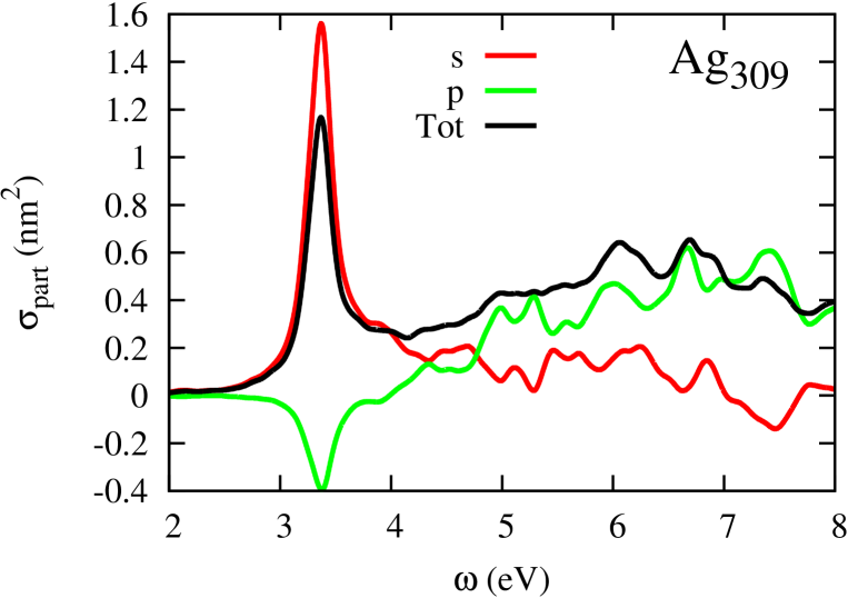
Figure 11: Analysis of the product-function angular-momentum contributions to the absorption cross section of the Ag₃₀₉ cluster. The total absorption cross-section is also plotted for comparison.

In figure 11, we present the analysis of the product-function angular momentum contributions to the optical absorption cross section. The partial cross sections corresponding to the partial polarizability (36) are plotted together with the total absorption cross section for Ag₃₀₉ cluster. The contribution of the angular momentum higher than $p$ is strictly zero. The contribution of $s$-symmetric product functions dominates in the cross section, while the contribution of $p$-symmetric functions is negative for the low-frequency resonance in the range 3–4 eV and positive in the frequency range 5–8 eV.

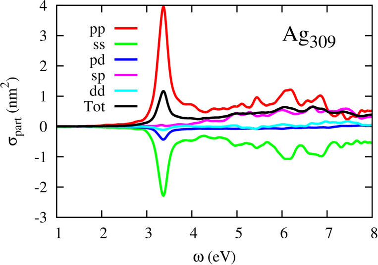
Figure 12: Analysis of atomic orbital angular momenta of the products of atomic-orbitals contributions to the optical absorption cross-section of the Ag₃₀₉ cluster. The total absorption cross-section is also plotted for comparison.

In the figure 12, we plot the partial cross sections computed from the orbital angular-momentum-resolved polarizability (38) for the 5-layered icosahedral cluster Ag₃₀₉. The sum of the partial cross sections is also shown for comparison. We can clearly appreciate the contribution of $p$-orbitals to the total absorption cross section. Namely, the contribution of the $pp$ angular-momentum channel is the most significant. The contributions have different signs and, for example, $pp$-products give rise to a partial cross section that is about 3 times larger than the total cross section. The second most important type of products is of $ss$ type. The partial cross section of $ss$ type is negative in the whole frequency range we computed. The absolute value of $ss$ partial cross section is about 1.7 times larger than the total cross section. The other non-zero angular-momentum channels do not contribute significantly to the total absorption cross section. Therefore, a linear combination of $pp$ and $ss$ products of atomic orbitals seems to be able to provide a reasonably accurate description of the total absorption cross section in the frequency range 0–10 eV and even better so in the frequency range 0–4 eV.

Appendix B GGA interaction kernel

In the generalized gradient approximation (GGA) of DFT functional, the xc energy density $\epsilon$ explicitly depends on the charge density $n(\bm{r})$ and its gradient $\nabla n(\bm{r})$

$$E=\int\epsilon(n(\bm{r}),\nabla n(\bm{r}))d^{3}r.$$ (40)

In the Kohn-Sham formulation of DFT we need the functional derivative of the energy with respect to the electron density

$$v(\bm{r})\equiv\frac{\delta E}{\delta n(\bm{r})}=\frac{\partial\epsilon}{\partial n}-\nabla\frac{\partial\epsilon}{\partial\nabla n}.$$ (41)

and in the linear response TDDFT we need also a second variational derivative of the energy with respect to the electronic density

$$f(\bm{r},\bm{r}^{\prime})\equiv\frac{\delta v(\bm{r})}{\delta n(\bm{r}^{\prime})}.$$ (42)

While the calculation of the KS potential in GGA is widely discussed in the literature [119, 120, 121], the TDDFT kernel (42) is less commonly discussed [122, 123] and we find it convenient to state explicitly the equations necessary for the implementation of our iterative TDDFT method.

B.1 Variational derivative of potential

In linear response TDDFT one needs a first variational derivative of the xc potential with respect to density (42). The potential (41) is in fact a functional of the density and its gradient. Computing the variation of the potential one gets

$$\delta v(\bm{r})=\frac{\partial^{2}\epsilon}{\partial n\partial n}\delta n+\frac{\partial^{2}\epsilon}{\partial n\partial\nabla_{i}n}\nabla_{i}\delta n - \nabla_{i}\left(\frac{\partial^{2}\epsilon}{\partial n\partial\nabla_{i}n}\delta n\right)$$ (43)

$$- \nabla_{i}\left(\frac{\partial^{2}\epsilon}{\partial\nabla_{k}n\partial\nabla_{i}n}\nabla_{k}\delta n\right).$$

In order to “exchange” the gradients of density variation $\nabla_{i}\delta n$ and $\nabla_{k}\nabla_{i}\delta n$ for the density variation $\delta n$, we represent the last equation in form of an integral with a $\delta$-function $\delta v(\bm{r}^{\prime})=\int\delta(\bm{r}^{\prime}-\bm{r})\delta v(\bm{r})d^{3}r$ and apply the integration by parts whenever necessary. Finally we can get [124]

$$\delta v(\bm{r}^{\prime}) = \int\delta(\bm{r}^{\prime}-\bm{r})\delta n\frac{\partial^{2}\epsilon}{\partial n\partial n}-\delta(\bm{r}^{\prime}-\bm{r})\delta n\nabla_{i}\left[\frac{\partial^{2}\epsilon}{\partial n\partial\nabla_{i}n}\right]$$ (44)

$$- \delta n\nabla_{k}\left[\nabla_{i}\left[\delta(\bm{r}^{\prime}-\bm{r})\right]\frac{\partial^{2}\epsilon}{\partial\nabla_{k}n\partial\nabla_{i}n}\right]d^{3}r.$$

By virtue of the kernel definition (42), the kernel GGA reads [125]

$$f(\bm{r},\bm{r}^{\prime})=\delta(\bm{r}-\bm{r}^{\prime})\frac{\partial^{2}\epsilon}{\partial n\partial n} - \delta(\bm{r}-\bm{r}^{\prime})\nabla_{i}\left[\frac{\partial^{2}\epsilon}{\partial n\partial\nabla_{i}n}\right]$$ (45)

$$- \nabla_{k}\left[\nabla_{i}\left[\delta(\bm{r}-\bm{r}^{\prime})\right]\frac{\partial^{2}\epsilon}{\partial\nabla_{k}n\partial\nabla_{i}n}\right].$$

B.2 Computation of GGA matrix elements of potential

In DFT, we need matrix elements of the xc potential (41)

$$v^{ab}=\int f^{a}(\bm{r})\frac{\partial\epsilon}{\partial n}f^{b}(\bm{r})d^{3}r-\int f^{a}(\bm{r})\nabla\frac{\partial\epsilon}{\partial\nabla n}f^{b}(\bm{r})d^{3}r$$ (46)

between the atomic orbitals $f^{a}(\bm{r})$. Because we use LIBXC library [126], we need to work with derivatives of the xc energy density with respect to the square of the density gradient, i.e. in terms of $\sigma\equiv(\nabla n)^{2}$. After applying the chain rule, we transform the last formula to

$$v^{ab}=\int f^{a}(\bm{r})\frac{\partial\epsilon}{\partial n}f^{b}(\bm{r})d^{3}r-2\int f^{a}(\bm{r})\nabla_{i}[\frac{\partial\epsilon}{\partial\sigma}\nabla_{i}n]f^{b}(\bm{r})d^{3}r,$$ (47)

Here and in the following the summation over repeated Cartesian indices ($i$ and $k$) is understood. The expression (47), similar to that in equation (46), is inconvenient in a numerical calculation because one must compute derivatives of the quantities delivered by LIBXC library ($\frac{\partial\epsilon}{\partial\nabla n}$ or $\frac{\partial\epsilon}{\partial\sigma}\nabla n$ ). However, with one more integration by parts, we can transform the expression (47) into a more suitable form

$$v^{ab}= \int f^{a}(\bm{r})\ \frac{\partial\epsilon}{\partial n}\ f^{b}(\bm{r})d^{3}r$$ (48)

$$+2\int\nabla_{i}[f^{a}(\bm{r})]\nabla_{i}n\ \frac{\partial\epsilon}{\partial\sigma}\ f^{b}(\bm{r})\,d^{3}r$$

$$+2\int f^{a}(\bm{r})\ \frac{\partial\epsilon}{\partial\sigma}\ \nabla_{i}[f^{b}(\bm{r})]\nabla_{i}n\,d^{3}r.$$

This form is advantageous because it is easier to calculate the gradients of the basis functions, the form of which is known and does not change with the type of the xc functional. Moreover, the last expression uses the same ingredients that are necessary to compute the matrix elements of GGA kernel.

B.3 Computation of GGA matrix elements of kernel

In our implementation of the linear response TDDFT, we need the matrix elements of the xc kernel (45) defined by $K^{\mu\nu}=\int F^{\mu}(\bm{r})f(\bm{r},\bm{r}^{\prime})F^{\nu}(\bm{r}^{\prime})d^{3}rd^{3}r^{\prime}$. Exercising the same approach as for the potential in the previous subsection, we obtain for matrix elements of GGA kernel

$$K^{\mu\nu}=\int F^{\mu}(\bm{r})\ \frac{\partial^{2}\epsilon}{\partial n^{2}} \ F^{\nu}(\bm{r})d^{3}r$$

$$+2\int\nabla_{i}[F^{\mu}(\bm{r})]\nabla_{i}[n]\ \frac{\partial^{2}\epsilon}{\partial n\partial\sigma} \ F^{\nu}(\bm{r})d^{3}r$$

$$+2\int F^{\mu}(\bm{r})\ \frac{\partial^{2}\epsilon}{\partial n\partial\sigma} \ \nabla_{i}[F^{\nu}(\bm{r})]\nabla_{i}[n]d^{3}r$$

$$+4\int\nabla_{k}[F^{\mu}(\bm{r})]\nabla_{k}[n]\ \frac{\partial^{2}\epsilon}{\partial\sigma^{2}} \ \nabla_{i}[F^{\nu}(\bm{r})]\nabla_{i}[n]d^{3}r$$

$$+2\int\nabla_{k}[F^{\mu}(\bm{r})]\ \frac{\partial\epsilon}{\partial\sigma} \ \delta_{ik}\nabla_{i}[F^{\nu}(\bm{r})]d^{3}r.$$ (49)

These matrix elements are computed with standard integration methods in quantum chemistry [127, 128].

References

- [1] de Heer W A 1993 Rev. Mod. Phys. 65(3) 611–676 URL http://link.aps.org/doi/10.1103/RevModPhys.65.611
- [2] 2015 Silver. Chemical Elements: From Carbon to Krypton. (Gale group) URL http://www.encyclopedia.com/doc/1G2-3427000094.html
- [3] Brack M 1993 Rev. Mod. Phys. 65(3) 677–732 URL http://link.aps.org/doi/10.1103/RevModPhys.65.677
- [4] Thämer M, Kartouzian A, Heister P, Lünskens T, Gerlach S and Heiz U 2014 Small 10 2340–2344 ISSN 1613-6829 URL http://dx.doi.org/10.1002/smll.201303158
- [5] Madison L R, Ratner M A and Schatz G C 2015 Understanding the electronic structure properties of bare silver clusters as models for plasmonic excitation Frontiers in Quantum Methods and Applications in Chemistry and Physics (Progress in Theoretical Chemistry and Physics vol 29) ed Nascimento M, Maruani J, Brändas E J and Delgado-Barrio G (Springer International Publishing) pp 37–52 ISBN 978-3-319-14396-5 URL http://dx.doi.org/10.1007/978-3-319-14397-2_3
- [6] Cushing S K and Wu N 0 The Journal of Physical Chemistry Letters 0 666–675 pMID: 26817500 (Preprint http://dx.doi.org/10.1021/acs.jpclett.5b02393) URL http://dx.doi.org/10.1021/acs.jpclett.5b02393
- [7] Kreibig U and Vollmer M 1995 Optical Properties of Metal Clusters (Springer Series in Materials Science vol 25) (Berlin: Springer) ISBN 978-3-642-08191-0 URL http://link.springer.com/book/10.1007%2F978-3-662-09109-8
- [8] Hao E and Schatz G C 2004 The Journal of Chemical Physics 120 357–366 URL http://scitation.aip.org/content/aip/journal/jcp/120/1/10.1063/1.1629280
- [9] Koponen L, Tunturivuori L O, Puska M J and Hancock Y 2010 The Journal of Chemical Physics 132 214301 URL http://scitation.aip.org/content/aip/journal/jcp/132/21/10.1063/1.3425623
- [10] Bousquet B, Cherif M, Huang K and Rabilloud F 2015 The Journal of Physical Chemistry C 119 4268–4277 (Preprint http://dx.doi.org/10.1021/jp512209p) URL http://dx.doi.org/10.1021/jp512209p
- [11] Kuisma M, Sakko A, Rossi T P, Larsen A H, Enkovaara J, Lehtovaara L and Rantala T T 2015 Phys. Rev. B 91(11) 115431 URL http://link.aps.org/doi/10.1103/PhysRevB.91.115431
- [12] Wiley B, Sun Y, Mayers B and Xia Y 2005 Chemistry – A European Journal 11 454–463 ISSN 1521-3765 URL http://dx.doi.org/10.1002/chem.200400927
- [13] Chang R and Leung P T 2006 Phys. Rev. B 73(12) 125438 URL http://link.aps.org/doi/10.1103/PhysRevB.73.125438
- [14] Oldenburg S J 2015 URL http://www.sigmaaldrich.com/materials-science/nanomaterials/silver-nanoparticles.html
- [15] Mathew A and Pradeep T 2014 Particle & Particle Systems Characterization 31 1017–1053 ISSN 1521-4117 URL http://dx.doi.org/10.1002/ppsc.201400033
- [16] Shimizu K i and Satsuma A 2006 Phys. Chem. Chem. Phys. 8(23) 2677–2695 URL http://dx.doi.org/10.1039/B601794K
- [17] Leelavathi A, Bhaskara Rao T and Pradeep T 2011 Nanoscale Research Letters 6 123 ISSN 1556-276X URL http://www.nanoscalereslett.com/content/6/1/123
- [18] Guável X L, Hötzer B, Jung G, Hollemeyer K, Trouillet V and Schneider M 2011 The Journal of Physical Chemistry C 115 10955–10963 (Preprint http://dx.doi.org/10.1021/jp111820b) URL http://dx.doi.org/10.1021/jp111820b
- [19] Chakraborty I, Udayabhaskararao T and Pradeep T 2012 Journal of Hazardous Materials 211–212 396 – 403 ISSN 0304-3894 nanotechnologies for the Treatment of Water, Air and Soil URL http://www.sciencedirect.com/science/article/pii/S030438941101524X
- [20] Qu F, Li N B and Luo H Q 2012 Analytical Chemistry 84 10373–10379 pMID: 23134573 (Preprint http://dx.doi.org/10.1021/ac3024526) URL http://dx.doi.org/10.1021/ac3024526
- [21] Chakraborty I, Bag S, Landman U and Pradeep T 2013 The Journal of Physical Chemistry Letters 4 2769–2773 (Preprint http://dx.doi.org/10.1021/jz4014097) URL http://dx.doi.org/10.1021/jz4014097
- [22] Birke R L and Lombardi J R 2015 Journal of Optics 17 114004 URL http://stacks.iop.org/2040-8986/17/i=11/a=114004
- [23] Hao F and Nordlander P 2007 Chemical Physics Letters 446 115 – 118 ISSN 0009-2614 URL http://www.sciencedirect.com/science/article/pii/S0009261407010986
- [24] Charlé K P, König L, Nepijko S, Rabin I and Schulze W 1998 Crystal Research and Technology 33 1085–1096 ISSN 1521-4079 URL http://dx.doi.org/10.1002/(SICI)1521-4079(199810)33:7/8<1085::AID-CRAT1085>3.0.CO;2-A
- [25] Negre C F A, Perassi E M, Coronado E A and Sánchez C G 2013 Journal of Physics: Condensed Matter 25 125304 URL http://stacks.iop.org/0953-8984/25/i=12/a=125304
- [26] Barbry M, Koval P, Marchesin F, Esteban R, Borisov A G, Aizpurua J and Sánchez-Portal D 2015 Nano Letters 15 3410–3419 pMID: 25915173 URL http://dx.doi.org/10.1021/acs.nanolett.5b00759
- [27] Aikens C M, Li S and Schatz G C 2008 The Journal of Physical Chemistry C 112 11272–11279 (Preprint http://dx.doi.org/10.1021/jp802707r) URL http://dx.doi.org/10.1021/jp802707r
- [28] Weissker H C, Whetten R L and Lopez-Lozano X 2014 Phys. Chem. Chem. Phys. 16(24) 12495–12502 URL http://dx.doi.org/10.1039/C4CP01277A
- [29] Barcaro G, Sementa L, Fortunelli A and Stener M 2014 The Journal of Physical Chemistry C 118 12450–12458 (Preprint http://dx.doi.org/10.1021/jp5016565) URL http://dx.doi.org/10.1021/jp5016565
- [30] Barcaro G, Broyer M, Durante N, Fortunelli A and Stener M 2011 The Journal of Physical Chemistry C 115 24085–24091 (Preprint http://dx.doi.org/10.1021/jp2087219) URL http://dx.doi.org/10.1021/jp2087219
- [31] Barcaro G, Sementa L, Fortunelli A and Stener M 2014 The Journal of Physical Chemistry C 118 28101–28108 (Preprint http://dx.doi.org/10.1021/jp508824w) URL http://dx.doi.org/10.1021/jp508824w
- [32] Baetzold R C 1978 The Journal of Chemical Physics 68 555–561 URL http://scitation.aip.org/content/aip/journal/jcp/68/2/10.1063/1.435765
- [33] Zhao J, Luo Y and Wang G 2001 The European Physical Journal D - Atomic, Molecular, Optical and Plasma Physics 14 309–316 ISSN 1434-6060 URL http://dx.doi.org/10.1007/s100530170197
- [34] Bonac̆ić-Koutecký V, Burda J, Mitrić R, Ge M, Zampella G and Fantucci P 2002 The Journal of Chemical Physics 117 3120–3131 URL http://scitation.aip.org/content/aip/journal/jcp/117/7/10.1063/1.1492800
- [35] Johnson H E and Aikens C M 2009 The Journal of Physical Chemistry A 113 4445–4450 (Preprint http://dx.doi.org/10.1021/jp811075u) URL http://dx.doi.org/10.1021/jp811075u
- [36] Lozano X L, Mottet C and Weissker H C 2013 The Journal of Physical Chemistry C 117 3062–3068 (Preprint http://dx.doi.org/10.1021/jp309957y) URL http://dx.doi.org/10.1021/jp309957y
- [37] Heard C J and Johnston R L 2014 Phys. Chem. Chem. Phys. 16(39) 21039–21048 URL http://dx.doi.org/10.1039/C3CP55507K
- [38] Baishya K, Idrobo J C, Öğüt S, Yang M, Jackson K and Jellinek J 2008 Phys. Rev. B 78(7) 075439 URL http://link.aps.org/doi/10.1103/PhysRevB.78.075439
- [39] Idrobo J C and Pantelides S T 2010 Phys. Rev. B 82(8) 085420 URL http://link.aps.org/doi/10.1103/PhysRevB.82.085420
- [40] Huda M N and Ray A K 2003 Phys. Rev. A 67(1) 013201 URL http://link.aps.org/doi/10.1103/PhysRevA.67.013201
- [41] Bae G T and Aikens C M 2012 The Journal of Physical Chemistry A 116 8260–8269 pMID: 22838848 (Preprint http://dx.doi.org/10.1021/jp305330e) URL http://dx.doi.org/10.1021/jp305330e
- [42] Koval P, Foerster D and Coulaud O 2010 J. Chem. Theo. Comput. 6 2654–2668 URL http://pubs.acs.org/doi/abs/10.1021/ct100280x
- [43] Koval P, Foerster D and Coulaud O 2010 physica status solidi (b) 247 1841–1848 ISSN 1521-3951 URL http://dx.doi.org/10.1002/pssb.200983811
- [44] Soler J M, Artacho E, Gale J D, García A, Junquera J, Ordejón P and Sánchez-Portal D 2002 Journal of Physics: Condensed Matter 14 2745 URL http://stacks.iop.org/0953-8984/14/i=11/a=302
- [45] Artacho E, Anglada E, Diéguez O, Gale J D, García A, Junquera J, Martin R M, Ordejón P, Pruneda J M, Sánchez-Portal D and Soler J M 2008 Journal of Physics: Condensed Matter 20 064208 URL http://stacks.iop.org/0953-8984/20/i=6/a=064208
- [46] Tsolakidis A, Sánchez-Portal D and Martin R M 2002 Phys. Rev. B 66(23) 235416 URL http://link.aps.org/doi/10.1103/PhysRevB.66.235416
- [47] Koval N E, Sánchez-Portal D, Borisov A G and no R D M 2013 Nuclear Instruments and Methods in Physics Research Section B: Beam Interactions with Materials and Atoms 317, Part A 56 – 60 ISSN 0168-583X proceedings of the 19th International Workshop on Inelastic Ion-Surface Collisions (IISC-19), Frauenchiemsee, Germany, 16-21 September 2012 URL http://www.sciencedirect.com/science/article/pii/S0168583X13002206
- [48] Iida K, Noda M, Ishimura K and Nobusada K 2014 The Journal of Physical Chemistry A 118 11317–11322 pMID: 25367153 (Preprint http://dx.doi.org/10.1021/jp5088042) URL http://dx.doi.org/10.1021/jp5088042
- [49] Xiang H, Zhang X, Neuhauser D and Lu G 2014 The Journal of Physical Chemistry Letters 5 1163–1169 pMID: 26274465 (Preprint http://dx.doi.org/10.1021/jz500216t) URL http://dx.doi.org/10.1021/jz500216t
- [50] Gao Y, Neuhauser D, Baer R and Rabani E 2015 The Journal of Chemical Physics 142 034106 URL http://scitation.aip.org/content/aip/journal/jcp/142/3/10.1063/1.4905568
- [51] Andrade X, Botti S, Marques M A L and Rubio A 2007 The Journal of Chemical Physics 126 184106 URL http://scitation.aip.org/content/aip/journal/jcp/126/18/10.1063/1.2733666
- [52] Hübener H and Giustino F 2014 Phys. Rev. B 89(8) 085129 URL http://link.aps.org/doi/10.1103/PhysRevB.89.085129
- [53] Manjavacas A, Marchesin F, Thongrattanasiri S, Koval P, Nordlander P, Sánchez-Portal D and García de Abajo F J 2013 ACS Nano 7 3635–3643 URL http://pubs.acs.org/doi/abs/10.1021/nn4006297
- [54] Dronskowski R 2005 Computational Chemistry of Solid State Materials (Weinheim: Wiley-VCH) ISBN 978-3-527-31410-2
- [55] Nogueira F, Marques M A L and Fiolhais C 2003 A primer in density functional theory Lecture Notes in Physics (Berlin: Springer) URL https://cds.cern.ch/record/1391332
- [56] Gross E K U and Burke K 2006 Basics of TDDFT vol 706 (Springer) chap 1, p 1 URL http://link.springer.com/chapter/10.1007/3-540-35426-3_1
- [57] Petersilka M, Gossmann U J and Gross E 1996 Phys. Rev. Lett. 76 1212
- [58] Gross E 2010 Time-dependent density-functional formalism Benasque 2010, Summer school lecture URL http://www.tddft.org/TDDFT2010/school/gross3.pdf
- [59] Onida G, Reining L and Rubio A 2002 Rev. Mod. Phys. 74(2) 601–659 URL http://link.aps.org/doi/10.1103/RevModPhys.74.601
- [60] Bauernschmitt R, Häser M, Treutler O and Ahlrichs R 1997 Chemical Physics Letters 264 573 – 578 ISSN 0009-2614 URL http://www.sciencedirect.com/science/article/pii/S0009261496013437
- [61] Hamel S, Casida M E and Salahub D R 2001 The Journal of Chemical Physics 114 7342–7350 URL http://scitation.aip.org/content/aip/journal/jcp/114/17/10.1063/1.1358865
- [62] te Velde G, Bickelhaupt F M, Baerends E J, Fonseca Guerra C, van Gisbergen S J A, Snijders J G and Ziegler T 2001 Journal of Computational Chemistry 22 931–967 ISSN 1096-987X URL http://dx.doi.org/10.1002/jcc.1056
- [63] Blase X and Ordejón P 2004 Phys. Rev. B 69(8) 085111 URL http://link.aps.org/doi/10.1103/PhysRevB.69.085111
- [64] Foerster D 2008 The Journal of Chemical Physics 128 034108 URL http://scitation.aip.org/content/aip/journal/jcp/128/3/10.1063/1.2821021
- [65] Foerster D and Koval P 2009 The Journal of Chemical Physics 131 044103 URL http://scitation.aip.org/content/aip/journal/jcp/131/4/10.1063/1.3179755
- [66] Blanco M A, Flórez M and Bermejo M 1997 Journal of Molecular Structure: {THEOCHEM} 419 19 – 27 ISSN 0166-1280 URL http://www.sciencedirect.com/science/article/pii/S0166128097001851
- [67] Koval P, Foerster D and Sánchez-Portal D 2014 Phys. Rev. B 89(15) 155417 URL http://link.aps.org/doi/10.1103/PhysRevB.89.155417
- [68] Ljungberg M P, Koval P, Ferrari F, Foerster D and Sánchez-Portal D 2015 Phys. Rev. B 92(7) 075422 URL http://link.aps.org/doi/10.1103/PhysRevB.92.075422
- [69] Ren X, Rinke P, Blum V, Wieferink J, Tkatchenko A, Sanfilippo A, Reuter K and Scheffler M 2012 New Journal of Physics 14 053020 URL http://stacks.iop.org/1367-2630/14/i=5/a=053020
- [70] Frayssé V, Giraud L, Gratton S and Langou J 2005 ACM Trans. Math. Softw. 31 228–238 ISSN 0098-3500 URL http://doi.acm.org/10.1145/1067967.1067970
- [71] URL http://www.netlib.org/blas/
- [72] Haas P, Tran F and Blaha P 2009 Phys. Rev. B 79(8) 085104 URL http://link.aps.org/doi/10.1103/PhysRevB.79.085104
- [73] Yabana K and Bertsch G F 1999 Phys. Rev. A 60(5) 3809–3814 URL http://link.aps.org/doi/10.1103/PhysRevA.60.3809
- [74] Rabilloud F 2014 The Journal of Chemical Physics 141 144302 URL http://scitation.aip.org/content/aip/journal/jcp/141/14/10.1063/1.4897260
- [75] Wu Z and Cohen R E 2006 Phys. Rev. B 73(23) 235116 URL http://link.aps.org/doi/10.1103/PhysRevB.73.235116
- [76] Perdew J P, Ruzsinszky A, Csonka G I, Vydrov O A, Scuseria G E, Constantin L A, Zhou X and Burke K 2008 Phys. Rev. Lett. 100(13) 136406 URL http://link.aps.org/doi/10.1103/PhysRevLett.100.136406
- [77] Mattsson A E and Armiento R 2009 Phys. Rev. B 79(15) 155101 URL http://link.aps.org/doi/10.1103/PhysRevB.79.155101
- [78] Tran F, Laskowski R, Blaha P and Schwarz K 2007 Phys. Rev. B 75(11) 115131 URL http://link.aps.org/doi/10.1103/PhysRevB.75.115131
- [79] Marini A, Del Sole R and Onida G 2002 Phys. Rev. B 66(11) 115101 URL http://link.aps.org/doi/10.1103/PhysRevB.66.115101
- [80] Durante N, Fortunelli A, Broyer M and Stener M 2011 The Journal of Physical Chemistry C 115 6277–6282 (Preprint http://dx.doi.org/10.1021/jp112217g) URL http://dx.doi.org/10.1021/jp112217g
- [81] Kuisma M, Ojanen J, Enkovaara J and Rantala T T 2010 Phys. Rev. B 82(11) 115106 URL http://link.aps.org/doi/10.1103/PhysRevB.82.115106
- [82] Weissker H C and Lopez-Lozano X 2015 Phys. Chem. Chem. Phys. 17(42) 28379–28386 URL http://dx.doi.org/10.1039/C5CP01177A
- [83] Talman J D 2009 Computer Physics Communications 180 332–338 URL http://dx.doi.org/10.1016/j.cpc.2008.10.003
- [84] Koval P and Talman J D 2010 Computer Physics Communications 181 2212–2213 URL http://dx.doi.org/10.1016/j.cpc.2010.08.024
- [85] Foerster D 2006 ArXiv Physics e-prints (Preprint physics/0612187)
- [86] Junquera J, Paz O, Sánchez-Portal D and Artacho E 2001 Phys. Rev. B 64(23) 235111 URL http://link.aps.org/doi/10.1103/PhysRevB.64.235111
- [87] Anglada E, M Soler J, Junquera J and Artacho E 2002 Phys. Rev. B 66(20) 205101 URL http://link.aps.org/doi/10.1103/PhysRevB.66.205101
- [88] García-Gil S, García A, Lorente N and Ordejón P 2009 Phys. Rev. B 79(7) 075441 URL http://link.aps.org/doi/10.1103/PhysRevB.79.075441
- [89] Mark E C 1995 Time-dependent density functional response theory for molecules Recent Advances in Density Functional Methods (Recent Advances in Computational Chemistry vol 1) ed Delano P C (World Scientific) pp 155–192 ISBN 978-981-02-2442-4 URL http://www.worldscientific.com/worldscibooks/10.1142/2914
- [90] Li Y and Ullrich C A 2015 Journal of Chemical Theory and Computation 0 null (Preprint http://dx.doi.org/10.1021/acs.jctc.5b00987) URL http://dx.doi.org/10.1021/acs.jctc.5b00987
- [91] Bahn S R and Jacobsen K W 2002 Comput. Sci. Eng. 4 56–66 ISSN 1521-9615
- [92] Kuo K 2002 Structural Chemistry 13 221–230 ISSN 1040-0400 URL http://dx.doi.org/10.1023/A%3A1015847520094
- [93] URL http://departments.icmab.es/leem/siesta/Databases/
- [94] Rivero P, García-Suárez V M, Pereniguez D, Utt K, Yang Y, Bellaiche L, Park K, Ferrer J and Barraza-Lopez S 2015 Computational Materials Science 98 372–389 ISSN 0927-0256 URL http://www.sciencedirect.com/science/article/pii/S0927025614007940
- [95] Otto A and Petri E 1976 Solid State Communications 20 823 – 826 ISSN 0038-1098 URL http://www.sciencedirect.com/science/article/pii/0038109876912837
- [96] Lucas A A, Henrard L and Lambin P 1994 Phys. Rev. B 49(4) 2888–2896 URL http://link.aps.org/doi/10.1103/PhysRevB.49.2888
- [97] Johnson P B and Christy R W 1972 Phys. Rev. B 6(12) 4370–4379 URL http://link.aps.org/doi/10.1103/PhysRevB.6.4370
- [98] Babar S and Weaver J H 2015 Appl. Opt. 54 477–481 URL http://ao.osa.org/abstract.cfm?URI=ao-54-3-477
- [99] Tiggesbäumker J, Köller L, Meiwes-Broer K H and Liebsch A 1993 Phys. Rev. A 48(3) R1749–R1752 URL http://link.aps.org/doi/10.1103/PhysRevA.48.R1749
- [100] Mochizuki S and Ruppin R 1993 Journal of Physics: Condensed Matter 5 135 URL http://stacks.iop.org/0953-8984/5/i=1/a=015
- [101] Haberland H 2013 Nature 494(7435) URL http://dx.doi.org/10.1038/nature11886
- [102] Kreibig U and Zacharias P 1970 Zeitschrift für Physik 231 128–143 ISSN 0044-3328 URL http://dx.doi.org/10.1007/BF01392504
- [103] Fedrigo S, Harbich W and Buttet J 1993 Phys. Rev. B 47(16) 10706–10715 URL http://link.aps.org/doi/10.1103/PhysRevB.47.10706
- [104] Harb M, Rabilloud F, Simon D, Rydlo A, Lecoultre S, Conus F, Rodrigues V and Félix C 2008 The Journal of Chemical Physics 129 194108 URL http://scitation.aip.org/content/aip/journal/jcp/129/19/10.1063/1.3013557
- [105] Conus F, Rodrigues V, Lecoultre S, Rydlo A and Félix C 2006 The Journal of Chemical Physics 125 024511 URL http://scitation.aip.org/content/aip/journal/jcp/125/2/10.1063/1.2219442
- [106] Barcaro G, Broyer M, Durante N, Fortunelli A and Stener M 2011 The Journal of Physical Chemistry C 115 24085–24091 (Preprint http://dx.doi.org/10.1021/jp2087219) URL http://dx.doi.org/10.1021/jp2087219
- [107] Rohrdanz M A, Martins K M and Herbert J M 2009 The Journal of Chemical Physics 130 054112 URL http://scitation.aip.org/content/aip/journal/jcp/130/5/10.1063/1.3073302
- [108] Silverstein D W and Jensen L 2010 The Journal of Chemical Physics 132 194302 URL http://scitation.aip.org/content/aip/journal/jcp/132/19/10.1063/1.3429883
- [109] Rao Y, Lei Y, Cui X, Liu Z and Chen F 2013 Journal of Alloys and Compounds 565 50 – 55 ISSN 0925-8388 URL http://www.sciencedirect.com/science/article/pii/S0925838813005288
- [110] Ewusi-Annan E 2010 Modeling the optical properties of metal nanoparticles and metal-molecule systems Ph.D. thesis The Pennsylvania State University, Lasse Jensen, Thesis Advisor Master of Science, ewusi@psu.edu URL https://etda.libraries.psu.edu/paper/11220/5692
- [111] Yugang S, Brian T M and Younan X 2002 Nano Letters 2 481–485 (Preprint http://dx.doi.org/10.1021/nl025531v) URL http://dx.doi.org/10.1021/nl025531v
- [112] Sun Y, Mayers B and Xia Y 2003 Advanced Materials 15 641–646 ISSN 1521-4095 URL http://dx.doi.org/10.1002/adma.200301639
- [113] Wiley B, Sun Y, Mayers B and Xia Y 2005 Chemistry – A European Journal 11 454–463 ISSN 1521-3765 URL http://dx.doi.org/10.1002/chem.200400927
- [114] Geddes C D (ed) 2010 Reviews in Plasmonics 2010 (Reviews in Plasmonics vol 2010) (Springer-Verlag New York) ISBN 978-1-4614-0883-3 URL http://www.springer.com/us/book/9781461408833#
- [115] Pattanayak S, Priyam A and Paik P 2013 Dalton Trans. 42(29) 10597–10607 URL http://dx.doi.org/10.1039/C3DT50684C
- [116] Sönnichsen C 2001 Plasmons in metal nanostructures Ph.D. thesis Ludwig-Maximilians-Universität München URL https://edoc.ub.uni-muenchen.de/2367/1/Soennichsen_Carsten.pdf
- [117] Sönnichsen C, Franzl T, Wilk T, von Plessen G, Feldmann J, Wilson O and Mulvaney P 2002 Phys. Rev. Lett. 88(7) 077402 URL http://link.aps.org/doi/10.1103/PhysRevLett.88.077402
- [118] Grigoryan V, Springborg M, Minassian H and Melikyan A 2013 Computational and Theoretical Chemistry 1021 197 – 205 ISSN 2210-271X clusters: From Dimers to Nanoparticles URL http://www.sciencedirect.com/science/article/pii/S2210271X13003095
- [119] White J A and Bird D M 1994 Phys. Rev. B 50(7) 4954–4957 URL http://link.aps.org/doi/10.1103/PhysRevB.50.4954
- [120] Bylander D and Kleinman L 1997 Journal of Computational Physics 136 599 – 602 ISSN 0021-9991 URL http://www.sciencedirect.com/science/article/pii/S0021999197957843
- [121] Balbás L C, Martins J L and Soler J M 2001 Phys. Rev. B 64(16) 165110 URL http://link.aps.org/doi/10.1103/PhysRevB.64.165110
- [122] Gaiduk A P 2013 Theory of Model Kohn-Sham Potentials and its Applications Ph.D. thesis University of Western Ontario Electronic Thesis and Dissertation Repository. Paper 1099
- [123] Caillie C V and Amos R D 2000 Chemical Physics Letters 317 159–164 ISSN 0009-2614 URL http://www.sciencedirect.com/science/article/pii/S0009261499013469
- [124] Nazarov V U Personal communications URL http://mbpt-domiprod.wikidot.com/calculation-of-gga-kernel
- [125] Nazarov V U and Vignale G 2011 Phys. Rev. Lett. 107(21) 216402 URL http://link.aps.org/doi/10.1103/PhysRevLett.107.216402
- [126] Marques M A, Oliveira M J and Burnus T 2012 Computer Physics Communications 183 2272 – 2281 ISSN 0010-4655 URL http://www.sciencedirect.com/science/article/pii/S0010465512001750
- [127] Delley B 1990 The Journal of Chemical Physics 92 508–517 URL http://scitation.aip.org/content/aip/journal/jcp/92/1/10.1063/1.458452
- [128] Krack M and Köster A M 1998 The Journal of Chemical Physics 108 3226–3234 URL http://scitation.aip.org/content/aip/journal/jcp/108/8/10.1063/1.475719