Information geometric analysis of phase transitions in complex patterns: the case of the Gray-Scott reaction-diffusion model

Abstract

The Fisher-Rao metric from Information Geometry is related to phase transition phenomena in classical statistical mechanics. Several studies propose to extend the use of Information Geometry to study more general phase transitions in complex systems. However, it is unclear whether the Fisher-Rao metric does indeed detect these more general transitions, especially in the absence of a statistical model. In this paper we study the transitions between patterns in the Gray-Scott reaction-diffusion model using Fisher information. We describe the system by a probability density function that represents the size distribution of blobs in the patterns and compute its Fisher information with respect to changing the two rate parameters of the underlying model. We estimate the distribution non-parametrically so that we do not assume any statistical model. The resulting Fisher map can be interpreted as a phase-map of the different patterns. Lines with high Fisher information can be considered as boundaries between regions of parameter space where patterns with similar characteristics appear. These lines of high Fisher information can be interpreted as phase transitions between complex patterns.

I Introduction

Phase transitions are ubiquitous in nature. They are a dramatic change in a system’s properties triggered by a minuscule shift in its environment. Phase transitions are often associated with spontaneous symmetry breaking, where the transition is between an unordered phase and an ordered, less symmetric phase Binder (1987). In simple models of phase transitions an order parameter is defined, which is zero in the unordered phase and non-zero in the ordered phase Binder (1987); Zinn-Justin (1989); Hohenberg and Krekhov (2014). This is the basis for a mean-field approach to phase transitions, where an expansion of the free energy in the order parameter is performed. Many powerful methods have been developed over the years to study phase transitions, especially in the study of universality in so-called second order (or critical) transitions, such as the Landau-Ginzburg theory Hohenberg and Krekhov (2014); Yukhnovskii (1987) and Wilson’s Renormalization Group approach Wilson (1974); Binder (1987); Zinn-Justin (1989). For those transitions the order parameter is continuous, thermodynamic quantities obey scaling laws in the vicinity of the critical point, and there is a diverging correlation length. For first order transitions, on the other hand, there is a jump in the value of the order parameter, there is no diverging correlation length and thus no scaling of the thermodynamic functions near the transition point. During the transition there can be a mixed phase with a stable interface between the two phases Binder (1987). The study of first order transitions is very important for complex systems, especially social or ecological complex systems, because the sudden jump between two phases (which is discontinuous) can be quite dramatic Villa Martín et al. (2015).

While the Ginzburg-Landau-Wilson approach has been tremendously successful in explaining universality in second-order phase transitions, it requires the definition of an order parameter. Different approaches, which do not require an order parameter, can be useful for cases where an order parameter is difficult to identify, or does not exist (e.g. Wegner (1971)). In one such approach we study the probabilistic description of the system while changing the parameters to bring the system across a transition. The statistical properties of the system in the different phases are very different. Therefore, at the phase transition the shape of the probability distribution function will change drastically. This is captured by the Fisher information matrix (FIM) through the Cramér-Rao bound Fisher (1922); Cramér (1946); Rao (1945); Cover and Thomas (2006). A compelling differential-geometric framework to study the changes that the probability distribution undergoes is Information Geometry (IG) Amari and Nagaoka (2000). In IG the family of probability distributions that are parametrized by a set of continuous parameters (designated here as the vector $\theta$) is seen as a differential manifold. The parameters form a coordinate system on the manifold, and distances are measured by the Fisher-Rao metric:

$$g_{\mu\nu}(\theta)=\langle\partial_{\mu}\ln p\,\partial_{\nu}\ln p\rangle$$ (1)

which is a positive semi-definite, symmetric matrix that changes covariantly under reparametrizations of the probability distribution $p(x;\theta)$. Here $\partial_{\mu}\equiv\partial/\partial\theta^{\mu}$ is a derivative with respect to one of the parameters, indexed by $\mu$. The IG of many models in statistical mechanics has been studied, e.g., in Ingarden et al. (1979); Ingarden and Janyszek (1982); Janyszek and Mrugala (1989, 1999); Janyszek (1990); Ruppeiner (1979, 1981, 1995); Ruppeiner and Davis (1990); Ruppeiner et al. (2012); Brody and Rivier (1995); Brody and Ritz (2003); Brody and Hook (2009); Janke et al. (2004). Of particular interest in these studies is the role of the scalar (Riemannian) curvature. It was shown to diverge at critical transition points and on the spinodal curve Brody and Hook (2009); Janke et al. (2004), thus effectively preventing geodesics from crossing into the unphysical area of phase space Kumar et al. (2012). See also Maity et al. (2015) for a general renormalization group analysis of IG near criticality.

A connection between phase transitions in IG and the Ginzburg-Landau-Wilson approach can be made when an order parameter $\phi_{\mu}$ is the derivative of a thermodynamic potential with respect to some thermodynamic variable $\theta^{\mu}$. Then there exists a collective variable $X_{\mu}(x)$ such that $\phi_{\mu}=-k_{B}T\langle X_{\mu}\rangle$ Yukhnovskii (1987); Prokopenko et al. (2011) and the Fisher information matrix can be shown to obey Prokopenko et al. (2011):

$$g_{\mu\nu}=-\frac{\partial\langle X_{\mu}\rangle}{\partial\theta^{\nu}}=\beta\frac{\partial\phi_{\mu}}{\partial\theta^{\nu}}$$ (2)

where $\beta=(k_{B}T)^{-1}$ is the inverse temperature, $k_{B}$ being Boltzmann’s constant. At second order phase transitions in the thermodynamic limit this derivative diverges and therefore a corresponding entry of the FIM also diverges.

When the system is finite, the Fisher information does not diverge but rather attains a maximum. The maximum of the Fisher information has been used to accurately find the phase transition point in finite systems Wang et al. (2011); Prokopenko et al. (2011) and as a definition of criticality in living systems Hidalgo et al. (2014).

We have two main goals for the current work: first to test a conjecture set forth by Prokopenko et al. in Prokopenko et al. (2011) that a divergence (or maximization) of the entries of the FIM can detect phase transitions even in the absence of an order parameter.

Second, to measure the Fisher information matrix without resorting to the underlying dynamics of the system and without assuming a specific parametric model for equation (1). This addresses the problem that often the microscopic dynamics of complex systems are unknown, and an analytic description of the probability density function is missing.

To accomplish these two goals we chose to study the specific example of the two dimensional Gray-Scott (GS) reaction diffusion model Gray and Scott (1984). We chose the GS model for its rich variety of spatial and spatio-temporal patterns Pearson (1993) and we consider the transitions between the different patterns as critical transitions. Among the different types of patterns one can find self-replicating spots Reynolds et al. (1994); Wei (2001); Wei and Winter (2003), spatio-temporal chaos Wang and Ouyang (2007), and labyrinthine patterns Jones and Gunaratne (1998). These were first systematically classified by Pearson Pearson (1993). Our goal is to use the Fisher information matrix to construct a phase map for the Gray-Scott model, where we expect areas with high values of the Fisher information to demarcate the different patterns. As a probabilistic description for the system we chose the blob-size distribution, which we take to be a function of the control parameters of the model $F$ and $k$ and which we estimate non-parametrically by using image processing on the resulting spatial $V$ concentration from our simulations.

The paper is organized as follows: in Section II we discuss the relationship between Fisher information and criticality, which forms the motivation for our approach. We revisit the arguments in Prokopenko et al. (2011) and extend them to our case. In Section III we introduce the Gray-Scott model and discuss some of its properties. In Section IV we present the results of the computations and in Section V we explain the methods we used to compute the Fisher information in this settings. Last we discuss our results in Section VI.

II Fisher Information and Criticality

In this section we summarize the derivation performed in Prokopenko et al. (2011) leading to Eq. (2) that relates order parameters and the entries of the Fisher information matrix. This derivation leads to the conjecture Prokopenko et al. (2011) that it is enough to consider the Fisher information matrix entries rather than order parameters and is presented here because it is important for our exposition.

The Gibbs ensemble can be generically written in the following way:

$$p(x;\theta)=\frac{1}{Z(\theta)}\exp\left[-\theta^{\mu}X_{\mu}(x)\right]$$ (3)

with $Z(\theta)$ set by normalization and with summation convention over repeated indices, which we use throughout the paper. For this distribution, the Fisher information Eq. (1) is Prokopenko et al. (2011):

$$g_{\mu\nu}(\theta)=\partial_{\mu}\partial_{\nu}\ln Z(\theta)=\partial_{\mu}\partial_{\nu}(-\beta G)$$ (4)

where $G$ is the Gibbs free energy. Performing the derivatives we obtain Eq. (2).

For many systems, the order parameter can be defined by introducing an external field $h$ to the free energy that couples to the order parameter $\phi$ Binder (1987). The canonical example being the magnetization that couples to the external magnetic field, so that $M=-\left(\frac{\partial A}{\partial h}\right)_{T}$. The external field being one of the external parameters $\theta^{\mu}$. We then have:

$$\phi=-{\left(\frac{\partial G}{\partial h}\right)}_{T}.$$ (5)

Setting $\theta^{\hat{\mu}}=h$ for a particular $\hat{\mu}$ we obtain:

$$\phi_{\hat{\mu}}=-\frac{\partial G}{\partial\theta^{\hat{\mu}}}=-k_{B}T\langle X_{\hat{\mu}}\rangle.$$ (6)

The meaning of Eq. (6) is that if an order parameter $\phi_{\hat{\mu}}$ is a derivative of the free energy $G$, then there exists a collective variable $X_{\hat{\mu}}(x)$ whose average is proportional to the order parameter Prokopenko et al. (2011). It is important to note that many models exist whose order parameter is indeed the average of a collective variable Prokopenko et al. (2011); Yukhnovskii (1987).

Combining equations (4) and (6) we obtain Eq. (2). This links the value of the entries of the Fisher information with the derivatives of the order parameters $\phi_{\mu}$ of the system. Since at phase transitions the order parameter or its derivatives becomes non-analytic we can expect the Fisher information matrix to have diverging entries at the phase transition point. For example, at a ferromagnetic transition point, with $(\theta^{1},\theta^{2})=(h,T)$, the diagonal elements of the Fisher information matrix are given by Prokopenko et al. (2011):

$$k_{B}Tg_{11}(h) ={\left(\frac{\partial\phi}{\partial h}\right)}_{T}=-{\left(\frac{\partial^{2}G}{\partial h^{2}}\right)}_{T}\equiv\chi_{T}\,;$$ (7)

$$k_{B}Tg_{22}(T) ={\left(\frac{\partial S}{\partial T}\right)}_{h}=-{\left(\frac{\partial^{2}G}{\partial T^{2}}\right)}_{h}\equiv\frac{C_{h}}{T}\,.$$ (8)

Since $g_{11}$ and $g_{22}$ are proportional to the magnetic susceptibility $\chi_{T}$ and heat capacity $C_{h}$ respectively, we expect both entries to diverge at the point of the magnetic second order phase transition Prokopenko et al. (2011). More generally, it is easy to show that Prokopenko et al. (2011)

$$g_{\mu\nu}(\theta)=\langle X_{\mu}X_{\nu}\rangle-\langle X_{\mu}\rangle\langle X_{\nu}\rangle.$$ (9)

This is also called the generalized susceptibility in statistical mechanics Hidalgo et al. (2014). This derivation led Prokopenko to propose that the maximization of the appropriate Fisher information matrix can detect phase transitions, without explicitly defining an order parameter Prokopenko et al. (2011).

The relation (2) suggests the introduction of an order parameter derived from the Fisher information by integrating it from one phase to the next, in the following way:

$$\int\limits_{\theta_{1}}^{\theta_{2}}g_{\mu\nu}(\theta)d\theta^{\nu}=\int\limits_{\theta_{1}}^{\theta_{2}}\frac{\partial\phi_{\mu}}{\partial\theta^{\nu}}d\theta^{\nu}=\int\limits_{\theta_{1}}^{\theta_{2}}d\phi_{\mu}=\phi_{\mu}(\theta_{1},\theta_{2}).$$ (10)

We absorbed the inverse temperature in the definition of $\theta$, and the integration path starts at $\theta_{1}$ which is in one phase and ends at $\theta_{2}$ which is in the other phase. In general this will depend on the integration path and the end-points.

While the derivation above assumes the form (3) for the probabilistic description of the system, the idea of Fisher information maximization at phase transition points can be generalized for other probabilistic descriptions based on the Cramér-Rao bound Cramér (1946); Rao (1945); Cover and Thomas (2006) that states that the variance an unbiased estimator $\hat{\theta}(x)$ is bounded from below by the inverse of the Fisher information. We make the following heuristic argument: when a system is said to undergo a phase transition, it means that there is an observable change in some aspect of the system (often having to do with the symmetries of the system). This means that the statistical properties of the system in the two phases differ significantly. For example, if we sample the energy per spin of an Ising spin system repeatedly in the high-temperature phase, we will obtain a broad distribution of energies. Conversely, at the low-temperature phase the energy distribution is very narrow, since in the low-temperature phase the spins are aligned and the system is in the ground state Wilson (1974). Thus, if we look at the probability density function describing these observables change as a function of the control parameter, it undergoes a drastic change in its functional form. This, in turn, implies that we can estimate the value of the control parameter at the phase transition point accurately, because of the large change in the behavior of the density function. According to the Cramér-Rao inequality, the inverse of the value of the Fisher information serves as a lower bound on the variance of the estimated parameter. If this parameter can be estimated accurately then this implies a high value of the Fisher information. We therefore surmise that under very general circumstances the Fisher information is maximized at phase transition points.

III The Gray-Scott Model

The Gray-Scott model is a non-linear reaction-diffusion model of two chemical species $U$ and $V$ with the reactions

$$U+2V \rightarrow 3V$$ (11)

$$V \rightarrow P.$$

$U$ is constantly supplied into the system and the inert product $P$ removed.

We can simulate the reaction using the law of mass action Hinrichsen (2000), where we assume that the rate of each reaction is proportional to the concentration of the reactants at each point. The resulting non-linear coupled differential equations are:

$$\frac{\partial u}{\partial t} =D_{u}\nabla^{2}u-uv^{2}+F(1-u)$$ (12)

$$\frac{\partial v}{\partial t} =D_{v}\nabla^{2}v+uv^{2}-(F+k)v$$

where $u=u(t,\mathbf{x})$, $v=v(t,\mathbf{x})$ are the (dimensionless) concentrations of the two chemical species, $\nabla^{2}$ is the Laplacian with respect to $\mathbf{x}$, $D_{u}$ and $D_{v}$ are diffusion coefficients of $u$ and $v$ respectively, $F$ represents the rate of the feed of $U$ and the removal of $U$, $V$ and $P$ from the system and $k$ is the rate of conversion of $V$ to $P$. In practice this is a model of chemical species in a gel reactor where the rate $F$ can be relatively easily modified, and $k$ is dependent on the temperature of the system. $D_{u}$ and $D_{v}$ are more difficult to change and we will consider them constant, with $D_{u}/D_{v}=2$.

III.1 Linear stability analysis

We start with the standard stability analysis for the homogeneous system (i.e. without diffusion). The Gray-Scott model has a trivial homogeneous steady state solution, referred to as the red state, at $[u_{R},v_{R}]=[1,0]$ which is always linearly stable for positive $F$ and $k$ Pearson (1993); Mazin et al. (1996). Under the condition that

$$d=1-4(F+k)^{2}/F>0$$ (13)

two additional homogeneous steady states solutions appear:

$$[u_{B},v_{B}]=\left[\frac{1}{2}(1-\sqrt{d}),\frac{1}{2}\frac{F}{F+k}(1+\sqrt{d})\right]$$ (14)

$$[u_{I},v_{I}]=\left[\frac{1}{2}(1+\sqrt{d}),\frac{1}{2}\frac{F}{F+k}(1-\sqrt{d})\right].$$ (15)

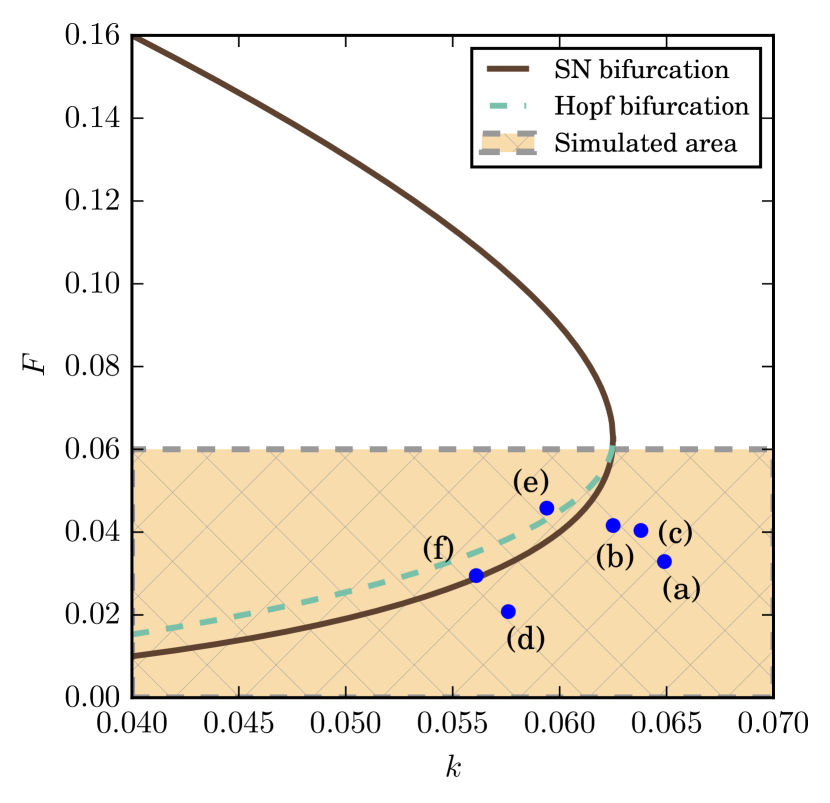
These are referred to as the blue state and the intermediate state respectively Mazin et al. (1996). Linear stability analysis shows that when these states exist, the intermediate state is always unstable whereas the blue state can be stable. The two states appear through a saddle-node bifurcation which in the $F-k$ plane is defined by the curve:

$$F_{SN}(k)=\frac{1}{8}\left[1-8k\pm\sqrt{1-16k}\right].$$ (16)

Under certain conditions Mazin et al. (1996) the blue state undergoes a Hopf bifurcation at

$$F_{H}(k)=\frac{1}{2}\left[\sqrt{k}-2k-\sqrt{k(1-4\sqrt{k})}\right].$$ (17)

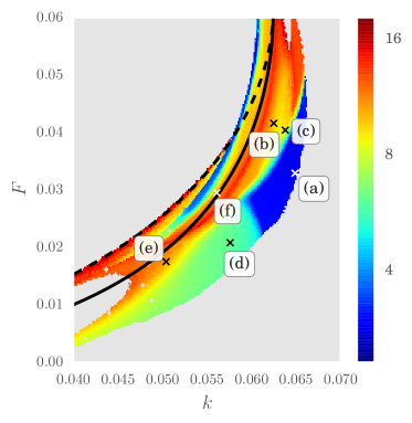
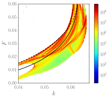
For more details see Mazin et al. (1996); Wei (2001); Wei and Winter (2003); McGough and Riley (2004). The bifurcation curves are plotted in Fig. 1 together with the area where we performed our simulations.

Figure 1: Bifurcation diagram of the Gray-Scott model. The solid line indicates the saddle-node bifurcation and the dashed line the Hopf bifurcation. The highlighted area is where we perform our simulations. The blue dots are the position in parameter space of the patterns that appear in Fig. 2.

III.2 Complex patterns

In the vicinity of the bifurcations a variety of inhomogeneous patterns may appear Mazin et al. (1996). These can be observed by setting the initial state of the system to the red state and adding a finite perturbation that allows the system to reach a different attractor (for details see Sec. V). The first to systematically study these patterns in two dimensions was Pearson Pearson (1993). Pearson classified the patterns in $12$ types and designated them with Greek letters. In this paper we use the same parameters Pearson used for his simulations, except that we will vary the simulation lattice size to include larger patterns, as will be described later. The different patterns appear close to each other in the $F-k$ space and often mix on the boundaries of regions of different patterns. One of the patterns that was first discovered by Pearson Pearson (1993) is that of the self-replicating spots (e.g. Fig. 2a). A single spot of high $V$ with a well defined boundary grows until at a certain point it will split into two spots. The process continues until the whole simulation area is covered with spots Reynolds et al. (1994). Depending on the parameters, the self-replicating spots will either reach an asymptotic fixed point or will start to flicker in what is known as spatio-temporal chaos Reynolds et al. (1994); Nishiura and Ueyama (1999, 2001); Wei (2001); Wei and Winter (2003). Wang and Ouyang Wang and Ouyang (2007) derived a probabilistic description of the spot count in the chaotic regime as a function of the rate of spot creation and annihilation which were found to linearly depend on the spot-count. Another group of patterns are the worm-like patterns (Fig. 2b) which grow and fill the entire simulation lattice and then are fixed. In the parameter space, between the stable self-replicating spots and the worm-like patterns, a mixed pattern appears which contains both spots and stripes. This pattern (Fig. 2c) is reminiscent of a first order phase transition, where phase co-existence appears in the transition region. The degree of mixing gradually increases and then decreases again across the transition.

(a) Self-replicating spots after replication is finished. $F=0.0392,k=0.0649$ (Pearson $\lambda$ pattern).

(b) Worm-like patterns. $F=0.0416,k=0.0625$ (Pearson $\mu$ pattern).

(c) “Mixed-phase” between the self-replicating spots and the worm-like pattern. $F=0.0404,k=0.0638$ (Pearson $\eta$ pattern).

(d) Spatio-temporal chaos (never reaches steady-state).$F=0.0208,k=0.0576$ (Pearson $\epsilon$ pattern).

(e) $F=0.0175,k=0.0504$ (Pearson $\alpha$ pattern).

(f) Labyrinthine pattern. $F=0.0295,k=0.0561$ (Pearson $\theta$ pattern).

Figure 2: Example of patterns found in the Gray-Scott model. These represent the concentration of $V$. All simulations performed with a grid size of $400\times 400$, and $D_{u}/D_{v}=2$.

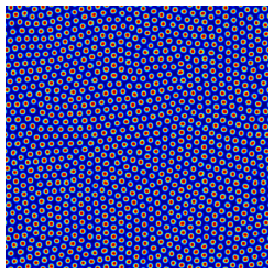
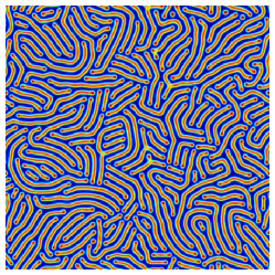
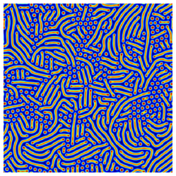
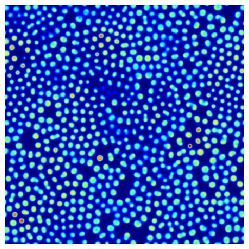
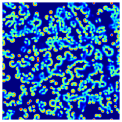
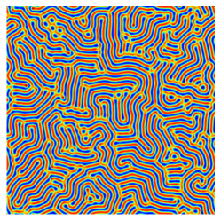
In the examples in Fig. 2, (a), (b), (c) and (f) patterns are at a fixed point of the dynamics. The patterns (d) and (e), on the other hand, are a snapshot of patterns that do not reach a fixed-point. The patterns that appear in the Gray-Scott are examples of self-organization because they are macroscopic patterns that appear through the local interactions of the $U$ and $V$ substances Prokopenko et al. (2009).

III.3 Probabilistic description

In order to construct a phase map using the Fisher information matrix, we follow Wang Wang and Ouyang (2007) in constructing our probabilistic description of the patterns. Wang treated each spot as an entity and computed the probability for a number of spots to appear at a unit time. We separate the pattern into similar entities, but regard not only the self-replicating spots but also the stripes and the labyrinthine patterns as entities, which we call “blobs”. 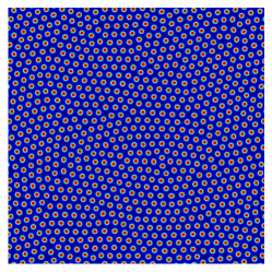We take the lattice of $V$ values (the $U$ value lattice is usually very similar to the $V$ one) and treat it as an image. To identify a blob we first binarize the image using Otsu’s methodOtsu (1975). 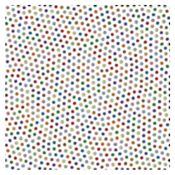We use the find_blobs method from the image processing python library SimpleCV  to label continuous clusters in the binarized image. 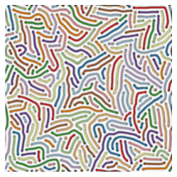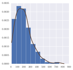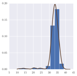We extract the size of each blob (in pixels) and use a non-parametric estimation procedure to obtain a PDF of the sizes of the blobs. We assume that the blob sizes are characteristic of the different patterns and that by observing their distribution we could, with a high degree of certainty, deduce the type of pattern. We therefore expect the Fisher information to become large when a PDF changes rapidly and therefore we will be able to detect the transitions between the patterns. The density extraction process is depicted in Fig. 3.

(a) Original image.

(b) Image with detected blobs superimposed.

(c) Histogram of blob areas with density estimation.

(d) Original image.

(e) Image with detected blobs superimposed.

(f) Histogram of blob areas with density estimation.

Figure 3: Two examples of the density extraction process. The original images 3a and 3d are binarized and a blob detection algorithm is run. This results in a set of blobs (depicted in 3b and 3e) from which a histogram of blob sizes is computed and a Gaussian kernel density estimation is used to obtain the final density function (plotted in 3c and 3f). First picture at $F=0.0413;\;k=0.0628$ and second picture at $F=0.0335;\;k=0.0644$.

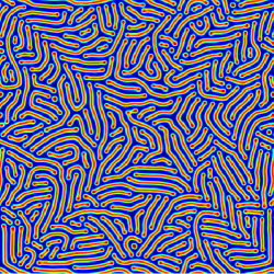
We assume that the extracted PDF is a function of the parameters $F$ and $k$ and that we can therefore compute derivatives of it with respect to these parameters by using a finite difference scheme. We use a centered finite difference scheme and the integration is performed by use of scipy.integrate.quad . The expression we use for the Fisher information is:

$$g_{\mu\nu}(\theta) =\int\frac{\ln p(x|\theta+\Delta\theta^{\mu})-\ln p(x|\theta-\Delta\theta^{\mu})}{2\Delta\theta^{\mu}}\times$$ (18)

$$\times\frac{\ln p(x|\theta+\Delta\theta^{\nu})-\ln p(x|\theta-\Delta\theta^{\nu})}{2\Delta\theta^{\nu}}p(x;\theta)\,dx.$$

In this expression $\Delta\theta^{\mu}$ represents a small increment in either $F$ or $k$, keeping the other fixed (so, for example, $\theta+\Delta\theta^{F}$ is interpreted as the probability density at $F+\Delta F,k$). Following Wang et al. (2011) we set the expression under the integration to zero whenever any of the densities was zero for a given $x$. An extended discussion about the use of non-parametric density estimation (such as Kernel Density Estimations) and using finite difference schemes in the computation of the Fisher information is given in Har Shemesh et al. (2015).

Since our premise is that the distribution of blob sizes is typical to the different patterns, we use the Shannon entropy, defined as:

$$H[p](\theta)\equiv\int p(x;\theta)\ln\frac{1}{p(x;\theta)}dx.$$ (19)

as a way to validate our method. The Shannon entropy (19) is a measure of uncertainty in the outcome of a random variable which is distributed according to $p(x;\theta)$. In our case it represents our uncertainty about the size of one of the blobs in the pattern. In the stable spots pattern, for example, the uncertainty is relatively low and so is the Shannon entropy. At the stripe pattern it is high, since any given blob can belong to a short or a long stripe. This gives us a sort of an order parameter which, however, is not necessarily related to a change in the symmetry of the system. This allows us to compare the predictions from the Fisher information to that of the Shannon entropy. We will typically expect a line of high Fisher information where the Shannon entropy undergoes a large change.

IV Results

IV.1 Two dimensional phase map

To get an overview of where in parameter space each patterns is located, we first plot the Shannon entropy of the blob-size PDF. The Shannon Entropy map for a simulation grid of $800\times 800$ is shown in Fig. 4. The Shannon entropy shows a clear demarcation between different regions in the parameter space near the saddle-node bifurcation curve. There are two areas with low entropy (blue regions, one above and one below the saddle-node curve). Both blue areas have stable localized spots of roughly the same size, but only the spots in the area containing the (a) pattern are created through self replication. The other spots are created with a different mechanism, see the Supplemental Material at for movies showing the evolution of these two patterns. When we move from the area containing (a) to the area containing (d) there is a well defined boundary where the blue region ends and where the spatio-temporal chaotic regime begins. The Shannon entropy increases slowly as one moves towards lower values of $F$ and $k$ since the size of the spots becomes less certain and since half formed spots are counted as blobs with smaller and more variable areas. We refer to this transition as “Transition I”. A second interesting transition occurs when moving from (a) to (b). In this transition the spots from pattern (a) mix with the stripes of pattern (b) to a varying degree, until there are no more spots and only stripes remain. As we can see the Shannon entropy increase is much steeper in this transition, since the blobs turn into stripes of wildly different lengths. We will refer to this transition as “Transition II”. Examples of transitions I and II can be seen in Figs. 6 and 7 respectively.

Figure 4: Shannon entropy of the blob size distribution. The black continuous line is the saddle-node bifurcation curve and the dashed line is the Hopf bifurcation. The Shannon Entropy was calculated for a simulation on an $800\times 800$ grid. The location of the different patterns from Fig. 2 are indicated with $\times$. The color-bar is in logarithmic scale. Gray indicates areas with no inhomogeneous patterns.

The different components of the Fisher information matrix and its trace and eigenvalues are plotted in Figure 5. At each point we computed the eigenvalues and plotted separately the larger eigenvalue (Fig. 5e) and the smaller one (Fig. 5f).

(a) $G_{FF}$ component.

(b) $G_{kk}$ component.

(c) $G_{Fk}$ component.

(d) $\mathrm{Tr\ }G$.

(e) Largest eigenvalue.

(f) Second eigenvalue of $G$.

Figure 5: The different components of the Fisher information matrix obtained for simulations with grid size $800\times 800$ and periodic boundary conditions. As can be seen from 5c, the off diagonal component is mostly negligible. The color in all figures is in logarithmic scale.

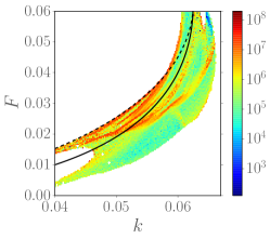
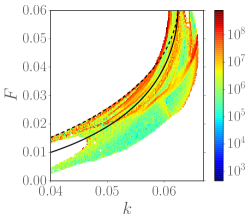
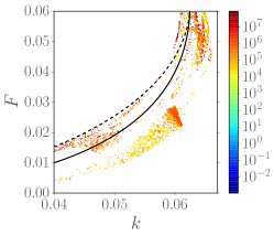
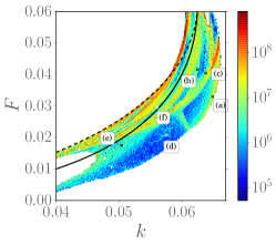
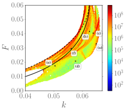
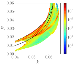
The main features of the Fisher information maps we see in Fig. 5 are that there are many curves with high values of the Fisher information (“ridges”) which separate areas of lower FI. Most ridges follow the general curve of the saddle-node bifurcation line, except for the noticeable ridge separating the self-replicating spots pattern region (a) and the spatio-temporal chaotic area (d) (i.e. the ridge representing Transition I). Almost all versions of the Fisher map show this ridge, but with a varying degree of clarity. Transition II is also clearly represented by a ridge which appears in almost all representations of the FIM (except for the $G_{Fk}$ component). This is the rather wide ridge where pattern (c) resides.

IV.2 One dimensional transitions

We constructed the two dimensional phase map by simulating the different patterns that appear in all the different parameter values we were interested in. Often we do not have complete knowledge of the surrounding patterns and only observe one instance of the system at a time. In these cases, it can be useful to look at a one dimensional plot of the Fisher information along a given trajectory. This can happen, for example, when we observe a natural system over time. Then we could treat the observation time as the parameter $\theta$ and compute how much we know about the observation time from the distribution $p$. As an example we plot the Shannon Entropy and the Fisher information interval along two trajectories. One crossing Transition I and the other Transition II. We define the Fisher information interval in analogy with special relativity D’Inverno (1992):

$$ds^{2}=G_{\mu\nu}d\theta^{\mu}d\theta^{\nu}.$$ (20)

It is an invariant measure that represents the squared distance along the path described by $d\theta^{\mu}$. To compute the interval we first defined the start and end of the path $\mathbf{p}_{1}=(k_{1},F_{1})$ and $\mathbf{p}_{2}=(k_{2},F_{2})$ respectively, then computed the unit vector connecting $\mathbf{p}_{1}$ and $\mathbf{p}_{2}$: $\mathbf{d\hat{r}}=(\mathbf{p}_{2}-\mathbf{p}_{1})/||\mathbf{p}_{2}-\mathbf{p}_{1}||$. And finally the vector $d\theta^{\mu}=(dk,dF)\cdot\mathbf{d\hat{r}}$. $dk$ and $dF$ are the lattice spacings in parameter space and $||\cdot||$ is the usual norm in $\mathbb{R}^{2}$.

IV.2.1 Transition I: self replicating spots to spatiotemporal chaos

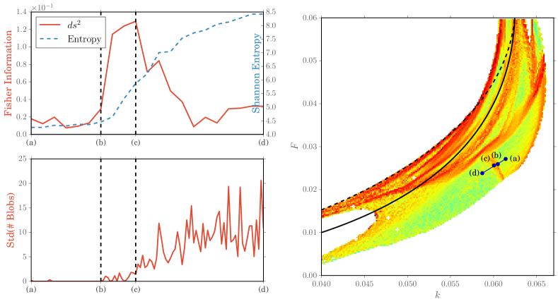
The first one dimensional transition we analyze is Transition I, which we define between the stable, self-replicating, spots and the chaotic spots. One such trajectory crossing the transition is plotted in Fig. 6. Point $(a)$ (at parameter values $k=0.06141,F=0.027136$) is located within the fixed spots area close to the transition and point $(d)$ (at parameter values $F=0.0238191,k=0.05869347$) is located within the chaotic spots area, also not far from the boundary. On the top left of Fig. 6 we plot the Fisher interval going from point $(a)$ to point $(d)$. At point $(b)$ the interval starts increasing and at point $(c)$ it reaches a maximum, after which is slowly decreases again. On the same graph we plot the Shannon entropy of the blob size PDF. The Shannon entropy is lower in the stable phase than in the spatio-temporal chaos, as can also be seen in Fig. 4. This is due to the increased uncertainty in blob sizes in the chaotic regime.

We inspected the patterns on both sides of the transition visually and as a function of time and it does indeed seem to capture the transition in the correct location. To verify this quantitatively we define an order parameter. Since the nature of the transition is dynamic (i.e. the time dependence of the pattern is different in both phases) we simulate the system further in time. We divide the trajectory from $(a)$ to $(d)$ to $100$ points at each point run the simulation for $50,000$ warm-up time steps for it to reach the state in which we computed the Fisher information. We then continue the simulation an additional $2,000$ time steps, computing the blob-count every $20$ time steps. From these samples we compute the standard deviation of the blob count. The rationale is that for the stable spots the variability of blob count should be zero and at the chaotic regime it is non-zero. This is plotted on the bottom left in Fig. 6, below the Fisher interval plot. We also plotted vertical lines that indicate the position of points $(b)$ and $(c)$. Because of the demanding computation time we performed the validation run on a $400\times 400$ grid as opposed to the $800\times 800$ grid from which the Fisher interval is computed. The blob-count indeed remains constant between $(a)$ and $(b)$. It then gradually becomes more variable as we go deeper into the chaotic regime. The increase in blob-count variability coincides with the rise in Fisher interval which we interpret as a verification that indeed the transition begins at this point.

Figure 6: One dimensional snapshot of Transition I, starting from point (a) to point (d), crossing the ridge defining the transition. Point (b) represents the onset of the rise of the Fisher information and point (c) represents the maximum of the Fisher information along the line. Top left figure - the line element $ds^{2}=G_{\mu\nu}d\theta^{\mu}d\theta^{\nu}$ connecting (a) and (c), and the Shannon entropy along the line. Bottom left plot represents the standard deviation in the blob count from a continued simulation along the line, as explained in the main text. The vertical dashed line in both plots represents the position of (b) and (c). The plot on the right is the same line element $ds^{2}$ plotted for the entire simulation region. The blue line is the line plotted on the left. Points (a), (b), (c), and (d) are also indicated.

IV.2.2 Transition II: self-replicating spots to stripes

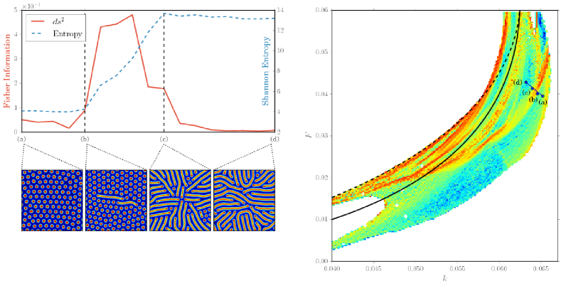
The second trajectory we chose crosses what we term Transition II. As the first transition, it starts in the self-replicating spots area (at a different point $(a)$ which is located at parameter values $k=0.0652$ and $F=0.0395$) and crosses to the area of the stripe patterns to point $(d)$ which is located at $k=0.0632,F=0.0428$. Along the trajectory the patterns evolve from completely spots to a mixed spot-stripe region and finally reach a region without any spots. Again we plot the trajectory in Fig. 7, along with the Fisher interval and Shannon entropy (top left). The Fisher interval clearly increases between points $(b)$ and $(c)$ which this time designate visually selected points of the start and end of the region where the Fisher interval is high. The Shannon entropy again increases across the transition and is higher in the stripe phase in comparison with the self-replicating spot phase. Below the Fisher interval and Shannon entropy plots we draw a part of the patterns that appear at points $(a)$ through $(d)$. This helps to provide a visual verification of the position of the transition. Point $(b)$ is the first point with stripes appearing together with the spots and point $(c)$ is one of the last with spots.

IV.2.3 Shannon Entropy and Fisher Information

It is tempting to compare the Shannon entropy and Fisher information in terms of how well they capture the transition. Both can be used as indicators, the Shannon entropy indicates a transition when its average value changes significantly and the Fisher information by rise and subsequent decrease in its value. We would like to note that, following the discussion earlier, the Fisher information acts as a susceptibility measure (as the magnetic susceptibility would act in an Ising model) and the Shannon entropy as an order parameter (as the magnetization would in an Ising model). We can however hypothesize that it is possible to find a transition between patterns in which the Shannon entropy is constant but the Fisher information peaks. For example, if the average blob size changes abruptly but the variance in blob sizes remains fixed. In that case the Shannon entropy would not catch the transition but the Fisher information would.

Figure 7: One dimensional snapshot of Transition II. Top left is a plot of the interval $ds^{2}=G_{\mu\nu}d\theta^{\mu}d\theta^{\nu}$ and the Shannon entropy along the line connecting point (a) in the stable self-replicating spots area and (d) in the stripes area. Points (b) and (c) represent the onset of increase of Fisher information and the point where the Shannon Entropy reached its maximal value. The images on the bottom represent zoomed-in depictions of the patterns appearing in all indicated points.

IV.3 Effect of the simulation grid size

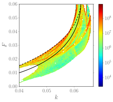
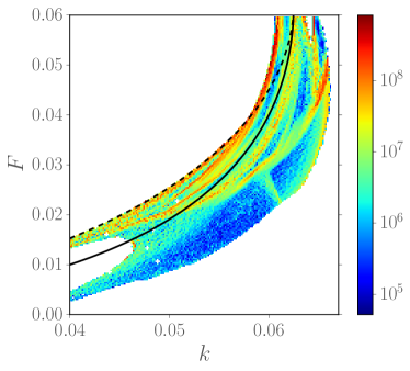
The size of the simulation grid, which we varied in our experiments from $256\times 256$ up to $1600\times 1600$ has a large effect on the resulting phase map. Small grid sizes result in a fairly noisy Fisher map, whereas larger ones give a smoother map with better defined “ridges” which demarcate the different phases. We suspect this is a result of too few blobs appearing in the smaller grids. Because simulating large grid sizes requires considerable computation time (the $1600\times 1600$ took about a month on a cluster running on approximately $800$ cores simultaneously), one has to find a balance between accuracy and computational time. We found that a grid size of $800\times 800$ provided good results.

In order to compare the results obtained for each of the grid sizes, we plot the trace of the Fisher information matrix obtained from the computation of the different grid sizes. This is presented in Fig. 8. At $256\times 256$ there is quite some noise from large peaks of the Fisher information. The $400\times 400$ grid already provides a much better resolution of the ridges, which improves even more at the $800\times 800$ grid. The $800\times 800$ grid also shows the highest contrast in Fisher information between “ridge” and “valley” regions. As we go to the largest grid size we used, $1600\times 1600$, it seems that some of the well-defined ridges become less well defined. We suspect that this might happen because the system did not have sufficient time to reach equilibrium, even though each simulation was run for $200,000$ time steps.

(a) Grid $256\times 256$

(b) Grid $400\times 400$

(c) Grid $800\times 800$

(d) Grid $1600\times 1600$

Figure 8: Comparison of different grid sizes. Trace of the FIM.

V Methods

The Fisher information is obtained by performing simulations on the parameter range where inhomogeneous patterns appear in the Gray-Scott model. The parameter space was divided into an evenly spaced $200\times 200$ grid with $F\in[0,0.06];\;k\in[0.04,0.07]$. The diffusion coefficients were held constant at $D_{u}=0.16;\;D_{v}=0.08$ such that $D_{u}/D_{v}=2$. We performed a simulation at each point of parameter space, starting with identical initial conditions (same seed) and repeated for the same number of time steps (depending on the simulation grid size). The simulation was started with an initial condition of the red state $(u,v)=(1,0)$ with a finite perturbation in the form of a $20\times 20$ square in the center of the simulation grid in the state $(u,v)=(0.5,0.25)$ and an additional Gaussian noise with an amplitude of $0.05$ covering the entire simulation grid. This initial state was then evolved by integrating numerically Eq. (12) using an Euler scheme until the final state was reached. We repeated the experiment with different simulation grid sizes, ranging between $200\times 200$ up to $1600\times 1600$. The simulation times ranged from $50,000$ time steps (for the smallest grid sizes) to $200,000$ for the $1600\times 1600$ grid. This was chosen such that the self-replicating stable spots will fill in the entire simulation window. The simulations were performed on the Lisa cluster run by SurfSara . The python code to perform the simulation is based on the code found at .

For each simulation we extracted the PDF by following the steps described in Section III.3. We used the Python package SimpleCV for the binarization and blob detection of the images and scipy.stats.gaussian_kde for the computation of the PDF from the blob sizes. The computation of the Fisher information from the PDF followed the description in Har Shemesh et al. (2015) and the code for this computation is available online at . As mentioned in Sec. IV we also computed the Shannon entropy for each PDF we obtained. This was done by simple integration of the PDF using Eq. (19) and the Python function scipy.integrate.quad.

In addition to the Gaussian KDE, we used the novel density estimation method DEFT Kinney (2014), and tried two different ways to integrate Eq. (18) - once as it is written in Eq. (18) and once by first performing the differentiation of the logarithm (replacing $\partial_{\mu}\ln p$ with $[1/p]\partial_{\mu}p$) before defining the finite difference scheme. As is described in Har Shemesh et al. (2015), the first method yields better results for Gaussian KDE and the second for DEFT. We eventually used the results obtained from the Gaussian KDE rather than the DEFT ones because finding the correct parameters for DEFT for all parameter values was difficult, since both the range of blob sizes and the number of blobs in each simulation in each parameter value varied too much.

VI Conclusions

In this paper we explore the use of the Fisher information matrix to capture transitions between different patterns in the Gray-Scott model. The use of Fisher information for this purpose is inspired by an analogy with phase transitions in thermodynamic systems and follows the work by Prokopenko et al. Prokopenko et al. (2011). The main purpose of the study was to test whether such a description is feasible in a system whose probabilistic description is not derived from the microscopic dynamics and where no statistical model is assumed. We find that at least in the case of the GS model with the choice of blob-size PDF as a probabilistic description, this seems to be indeed possible.

The main difficulty in using this approach to produce the entire phase map is that it is computationally very demanding. The very smooth phase map only really appears at grid sizes of $800\times 800$ which requires long computation runs. A more conceptual difficulty is that once we obtain the maps, their exact interpretation is not trivial. The value of the Fisher information ranges over many orders of magnitude (between $10^{3}$ and $10^{9}$) and there is no theoretical value to compare with.

The strength of the method lies in that it manages to capture various types of transitions with the same metric. We did not have to define specific order parameters for the different patterns. It also captures our intuitive understanding of a “phase transition” as a large change in the statistical properties of a system when the underlying “external” parameters are changed.

In the one-dimensional cases, it seems that the Fisher information does indeed capture essential features of “pattern transitions” in that it gives a clear signal in the form of a peak between two regions of low Fisher information. It is especially interesting to note that the Fisher information predicts an exact position for the transition to spatio-temporal chaos, as depicted in Fig. 6, since this transition is dynamic in nature. Further mathematical analysis similar to the one done in Nishiura and Ueyama (1999, 2001) for the two-dimensional Gray-Scott model might be able to confirm the exact position of the transition line and compare it to the one detected by the FI.

Our results suggest that Fisher information can indeed serve as a generalized susceptibility measure in the study of complex systems. Because very few assumptions about the underlying dynamics are necessary it is an ideal tool for detecting different regimes even in the absence of an assumed statistical model.