TECHNICAL REPORT
Parallel and sequential reclaiming in multicore real-time global scheduling

Abstract

When integrating hard, soft and non-real-time tasks in general purpose operating systems, it is necessary to provide temporal isolation so that the timing properties of one task do not depend on the behaviour of the others. However, strict budget enforcement can lead to inefficient use of the computational resources in the presence of tasks with variable workload. Many resource reclaiming algorithms have been proposed in the literature for single processor scheduling, but not enough work exists for global scheduling in multiprocessor systems. In this report we propose two reclaiming algorithms for multiprocessor global scheduling and we prove their correctness.

1 Introduction

The Resource Reservation Framework [18, 1] is an effective technique to integrate the scheduling of real-time tasks in general-purpose systems, as demonstrated by the fact that it has been recently implemented in the Linux kernel [12]. One of the most important properties provided by resource reservations is temporal isolation: the worst-case performance of a task does not depend on the temporal behaviour of the other tasks running in the system. This property can be enforced by limiting the amount of time for which each task can execute in a given period.

In some situations, a strict enforcement of the executed runtime (as done by the hard reservation mechanism that is currently implemented in the Linux kernel) can be problematic for tasks characterized by highly-variable, or difficult to predict, execution times: allocating the budget based on the task’ Worst Case Execution Time (WCET) can result in a waste of computational resources; on the other hand, allocating it based on a value smaller than the WCET can cause a certain number of deadline misses. These issues can be addressed by using a proper CPU reclaiming mechanism, which allows tasks to execute for more than their reserved time if spare CPU time is available and if this over-execution does not break the guarantees of other real-time tasks.

While many algorithms (e.g., [16, 13, 9, 15]) have been developed for reclaiming CPU time in single-processor systems, the problem of reclaiming CPU time in multiprocessor (or multicore) systems has been investigated less. Most of the existing reclaiming algorithms (see [13] for a summary of some commonly used techniques) are based on keeping track of the amount of execution time reserved to some tasks, but not used by them, and by distributing it between the various active tasks. In a multiprocessor system, this idea can be extended in two different ways:

1. by considering a global variable that keeps track of the execution time not used by all the tasks in the system (without considering the CPUs/cores on which the tasks execute), and by distributing such an unused execution time to the tasks. This approach will be referred to as parallel reclaiming in this paper, because the execution time not used by one single task can be distributed to multiple tasks that execute in parallel on different CPUs/cores;

2. by considering multiple per-CPU/core (per-runqueue, in the Linux kernel slang) variables each representing the unused bandwidth that can be distributed to the tasks executing on the corresponding CPU/core. This approach will be referred to as sequential reclaiming in this paper, because the execution time not used by one single task is associated to a CPU/core, and cannot be distributed to multiple tasks executing simultaneously.

This paper compares the two mentioned approaches by extending the GRUB (Greedy Reclamation of Unused Bandwidth) [15] reclaiming algorithm to support multiple processors according to sequential reclaiming and parallel reclaiming. The comparison is performed both from the theoretical point of view (by formally analysing the schedulability of the obtained algorithm) and by running experiments on a real implementation of this extension, named M-GRUB. Such implementation of M-GRUB reclaiming (that can do either parallel or sequential reclaiming) is based on the Linux kernel and extends the SCHED_DEADLINE scheduling policy.

The report is organised as follows: in Section 2 we recall the related work. In Section 3 we present our system model and introduce the definitions and concepts used in the paper. The algorithms and admission tests used as a starting point for this work are then presented in Section 4. The two proposed reclaiming rules are described in Section 5. In Section 6 we prove the correctness of the two algorithms. Finally, in Section 7 we present our conclusions.

2 Related work

The problem of reclaiming unused capacity for resource reservation algorithms has been mainly addressed in the context of single processor scheduling.

The CASH (CApacity SHaring) algorithm [9] uses a queue of unused budgets (also called capacities) that is exploited by the executing tasks. However, the CASH algorithm is only useful for periodic tasks. Lin and Brandt proposed BACKSLASH [13], a mechanism based on capacities that integrates four different principles for slack reclaiming. Similar techniques still based on capacities are used by Nogueira and Pinho [16].

The GRUB algorithm [15] modifies the rates at which servers’ budgets are decreased so to take advantage of free bandwidth. The algorithm can be also used by aperiodic tasks. We present the GRUB algorithm in Section 4 as it is used as a basis for our multiprocessor reclaiming schemes. For fixed priority scheduling, Bernat et al. proposed to reconsider past execution so to take advantage of the executing slack [5].

Reclaiming CPU time in multiprocessor systems is more difficult (especially if global scheduling is used), as shown by some previous work [8] that ends up imposing strict constraints on the distribution of spare budgets to avoid compromising timing isolation: spare CPU time can only be donated by hard real-time tasks to soft real-time tasks – which are scheduled in background respect to hard tasks – and reservations must be properly dimensioned.

To the authors’ best knowledge, the only previous algorithm that explicitly supports CPU reclaiming on all the real-time tasks running on multiple processors without imposing additional constraints (and has been formally proved to be correct) is M-CASH [17]. It is an extension of the CASH algorithm to the multiprocessor case, which additionally includes a rule for reclaiming unused bandwidth by aperiodic tasks. The algorithm uses the utilisation based test by Goossens, Funk and Baruah [10] as a base schedulability test for the servers. It distinguishes two kinds of servers: servers for periodic tasks (whose utilisation is reclaimed using capacity-based mechanism) and servers for aperiodic tasks, whose bandwidth is reclaimed with a technique similar to the parallel reclaiming that we propose in Section 5.1. However, M-CASH has never been implemented in a real OS kernel. On the other hand, the GRUB algorithm [15] has been implemented in the Linux kernel [2], after extending the algorithm to support multiple CPUs, but the multiprocessor extensions used in this implementation have not been formally analysed nor validated from a theoretical point of view.

3 System model and definitions

We consider a set of $n$ real-time tasks $\tau_{i}$ scheduled by a set of $n$ servers $S_{i}$ ($i=1,\dots,n$).

A real-time task $\tau_{i}$ is a (possibly infinite) sequence of jobs $J_{i,k}$: each job has an arrival time $a_{i,k}$, a computation time $c_{i,k}$ and a deadline $d_{i,k}$. Periodic real-time tasks are characterised by a period $T_{i}$, and their arrival time can be computed as $a_{i,k+1}=a_{i,k}+T_{i}$. Sporadic real-time tasks wait for external events with a minimum inter-arrival time, also called $T_{i}$, so $a_{i,k+1}\geq a_{i,k}+T_{i}$. Periodic and sporadic tasks are usually associated a relative deadline $D_{i}$ such that $d_{i,k}=a_{i,k}+D_{i}$.

A server is an abstract entity used by the scheduler to reserve a fraction of CPU-time to a task. Each server $S_{i}$ is characterised by the following parameters: $P_{i}$ is the server period and it represents the granularity of the reservation; $U_{i}$ is the fraction of reserved CPU-time, also called utilisation factor or bandwidth. In each period, a server is reserved at least a maximum budget, or runtime, $Q_{i}=U_{i}P_{i}$.

The execution platform consists of $m$ identical processors (Symmetric Multiprocessor Platform, or SMP). In this paper we use the Global Earliest Deadline First (G/EDF) scheduling algorithm: all the tasks are ordered by increasing deadlines of the servers, and the $m$ active tasks with the earliest deadlines are scheduled for execution on the $m$ CPUs.

The logical priority queue of G-EDF is implemented in Linux by a set of runqueues, one per each CPU/core, and some accessory data structures for making sure that the $m$ highest-priority jobs are executed at each instant (see [11] for a description of the implementation).

4 Background

In this section we first recall the Constant Bandwidth Server (CBS) algorithm [1, 3] for both single and multiprocessor systems. We then recall the GRUB algorithm [15], an extension of the CBS. Finally, we present two schedulability tests for Global EDF.

4.1 CBS and GRUB

As anticipated in Section 3, each server is characterised by a period $P_{i}$, a bandwidth $U_{i}$ and a maximum budget $Q_{i}=U_{i}P_{i}$. In addition, each server maintains the following dynamic variables: the server deadline $d_{i}$, denoting at every instant the server priority, and the server budget $q_{i}$, indicating the remaining computation time allowed in the current server period.

At time $t$, a server can be in one of the following states: ActiveContending, if there is some job of the served task that has not yet completed; ActiveNonContending, if all jobs of the served task have completed, but the server has already consumed all the available bandwidth (see the transition rules below for a characterisation of this state); Inactive, if all jobs of the server’s task have completed and the server bandwidth can be reclaimed (see the transition rules below), and Recharging, if the server has jobs to execute, but the budget is currently exhausted and needs to be recharged (this state is generally known as “throttled” in the Linux kernel, or “depleted” in the real-time literature).

Figure 1: State transition diagram for CBS and GRUB.

The states and the corresponding transitions are shown in Figure 1.

The EDF algorithm chooses for execution the $m$ tasks with the earliest server deadlines among the ActiveContending servers. Initially, all servers are in the Inactive state and their state change according to the following rules:

1. When a job of a task arrives at time $t$, if the corresponding server is Inactive, it goes in ActiveContending and its budget and deadlines are modified as: $q_{i}\leftarrow U_{i}P_{i}$ and $d_{i}\leftarrow t+P_{i}$

2. When a job of $S_{i}$ completes and there is another job ready to be executed, the server remains in ActiveContending with all its variables unchanged;

3. When a job of $S_{i}$ completes, and there is no other job ready to be executed, the server goes in ActiveNonContending.

4. If at some time $t$ the budget $q_{i}$ is exhausted, the server moves to state Recharging, and it is removed from the ready queue. The corresponding task is suspended and a new server is executed.

5. When $t=d_{i}$, the server variables are updated as $d_{i}\leftarrow d_{i}+P_{i}$ and $q_{i}\leftarrow U_{i}P_{i}$. The server is inserted in the ready queue and the scheduler is called to select the earliest deadline server, hence a context switch may happen.

6. If a new job arrives while the server is in ActiveNonContending, the server moves to ActiveContending without changing its variables.

7. A server remains in ActiveNonContending only if $q_{i}<(d_{i}-t)U_{i}$. When $q_{i}\geq(d_{i}-t)U_{i}$ the server moves to Inactive.

Only servers that are ActiveContending can be selected for execution by the EDF scheduler. If $S_{i}$ does not execute, its budget is not changed. When $S_{i}$ is executing, its budget is updated as $\operatorname{d}\!{q_{i}}=-\operatorname{d}\!{t}$.

When serving a task, a server generates a set of server jobs, each one with an arrival time, an execution time and a deadline as assigned by the algorithm’s rules. For example, when the server at time $t$ moves from Inactive to ActiveContending  a new server job is generated with arrival time equal to $t$, deadline equal to $d_{i}=t+P_{i}$, and worst-case computation time equal to $Q_{i}$. A similar thing happens when the server moves from Recharging to ActiveContending, and so on.

We say that a server is schedulable if every server job can execute the budget $Q_{i}$ before the corresponding server job deadline. It can be proved that the demand bound function $\mathsf{dbf}$ (see [4] for a definition) generated by the server jobs of $S_{i}$ is bounded from above as follows: $dbf(t)\leq U_{i}t$ for each $t$. Hence, for single processor systems it is possible to use the utilisation test of EDF as an admission control test, i.e.,

$$\sum_{i=1}^{n}U_{i}\leq 1.$$ (1)

We recall the following two fundamental results.

Theorem 1 (Theorem 1 in [1]).

If Equation (1) holds, then all server jobs meet their deadlines (i.e., all servers are schedulable).

Theorem 2 (Lemma 1 in [1]).

Assuming that Equation (1) holds, if a periodic (sporadic) hard real/time tasks with WCET $C_{i}$ and period (minimum inter/arrival time) $T_{i}$ is assigned a server with budget $Q_{i}\geq C_{i}$ and period $P_{i}\leq T_{i}$, then the task will meet all its deadlines.

The CBS algorithm has been extended to multiprocessor global scheduling in [3]. The authors prove the temporal isolation and the hard schedulability properties of the algorithm when using the schedulability test of Goossens, Funk and Baruah [10], which we will recall next.

The GRUB algorithm [15] extends the CBS algorithm by enabling the reclaiming of unused bandwidth, while preserving the schedulability of the served tasks. The main difference between the CBS and GRUB algorithms is the rule for updating the budget. In the original CBS algorithm, the server budget is updated as $\operatorname{d}\!{q_{i}}=-\operatorname{d}\!{t}$, independently of the status of the other servers. To reclaim the excess bandwidth, GRUB maintains one additional global variable $U_{\mathsf{act}}$, the total utilisation of all active servers

$$U_{\mathsf{act}}\coloneqq\sum_{S_{i}\notin\mbox{{\sf Inactive}}}U_{i}$$

and uses it to update the budget $q_{i}$ as

$$\cfrac{\operatorname{d}\!{q_{i}}}{\operatorname{d}\!{t}}=-(1-(U_{\mathsf{sys}}-U_{\mathsf{act}}))$$ (2)

where $U_{\mathsf{sys}}$ is the utilisation that the system reserves to the set of all servers. As in the original CBS algorithm, the budget is not updated when the server is not executing. The executing server gets all the free bandwidth in a greedy manner, hence the name of the algorithm. The GRUB algorithm preserves the Temporal Isolation and Hard Schedulability properties of the CBS [14].

4.2 Admission control tests

When using the CBS or the GRUB algorithm it is important to run an admission test to check if all the servers’ deadlines are respected. In single processor systems, the utilisation based test of Equation (1) is used for both the CBS and the GRUB algorithm. We now present two different schedulability tests for the multiprocessor case: an utilisation-based schedulability test for G-EDF by Goossens, Funk and Baruah [10] (referred to as GFB in this paper), and an interference-based schedulability test for G-EDF proposed by Bertogna, Cirinei and Lipari [7] (referred to as BCL in this paper).

GFB and BCL are not the most advanced tests in the literature: in particular, as discussed in [6], more effective tests – i.e. tests that can admit a larger number of task sets – are now available. The reason we chose these two in particular is their low complexity (so they can be used as on-line admission tests), and the fact that currently we are able to prove the correctness of the reclaiming rules with respect to these two tests in particular. In fact, we need to guarantee that the temporal isolation property continues to hold even when some budget is donated by one server to the other ones according to some reclaiming rule.

Currently, we have formally proved the correctness of the two reclaiming rules propose in Section 5 with respect to the GFB and the BCL test – see Section 6. Using some other, more effective, admission control test may be unsafe, hence, for the moment we restrict our attention to GFB and BCL.

The GFB test is based on the notion of uniform multiprocessor platform, and it allows to check the schedulability of a task set based on its utilisation.

Definition 1.

A uniform multiprocessor platform is comprised of several processors. Each processor $p$ is characterised by its speed $\mathsf{speed}(p)$, with the interpretation that a job that executes on processor $p$ for $t$ times units, completes $\mathsf{speed}(p)\cdot t$ units of execution. Let $\pi$ denote the uniform multiprocessor platform. We introduce the following notation:

$$\mathsf{MaxSpeed}_{\pi} \coloneqq\max_{p\in\pi}\{\mathsf{speed}(p)\}$$ (3)

$$\mathsf{TotSpeed}_{\pi} \coloneqq\sum_{p\in\pi}\mathsf{speed}(p).$$ (4)

Given a set of periodic (sporadic) tasks, we can always build a uniform multiprocessor platform on which the task set is schedulable, by providing one processor of speed $U_{i}$ per each task. This uniform multiprocessor platform will have $\mathsf{MaxSpeed}_{\pi}=\max_{i=1}^{n}\{U_{i}\}$ and $\mathsf{TotSpeed}_{\pi}=\sum_{i=1}^{n}U_{i}$.

Definition 2.

Let $I$ denote any set of jobs, and $\pi$ any uniform multiprocessor platform. For any scheduling algorithm A, and time instant $t\geq 0$, let $W(A,\pi,I,t)$ denote the amount of work done by algorithm A on jobs of I over the interval $[0,t)$ while executing on $\pi$.

The most general form of the test is given by the following Lemma.

Lemma 1 (Lemma $1$ in [10].).

Let $\pi$ denote a uniform multiprocessor platform with cumulative processor capacity $\mathsf{TotSpeed}_{\pi}$ and in which the fastest processor has speed $\mathsf{MaxSpeed}_{\pi}<1$. Let $\pi^{\prime}$ denote an identical multiprocessor platform comprised of $m$ processors of unit speed. Let A denote any uniform multiprocessor algorithm, and A’ any work conserving scheduling algorithm on $\pi$. If the following condition is satisfied:

$$m>\frac{\mathsf{TotSpeed}_{\pi}-\mathsf{MaxSpeed}_{\pi}}{1-\mathsf{MaxSpeed}_{\pi}}$$ (5)

then for any collection of jobs $I$ and any time instant $t\geq 0$,

$$W(A^{\prime},\pi^{\prime},I,t)\geq W(A,\pi,I,t)$$ (6)

The following theorem specializes the result of Lemma 1 for G-EDF.

Theorem 3 (Theorem $3$ in [10]).

Let $\pi$ denote a uniform multiprocessor platform as in Lemma 1. Let $i$ denote a set of jobs that is feasible in $\pi$. Let $\pi^{\prime}$ an identical multiprocessor platform comprised of $m$ unit-speed processors. If Equation (5) is satisfied, then $I$ will meet all deadlines when scheduled using G-EDF on $\pi^{\prime}$.

In practice, according to GFB, a set of periodic or sporadic tasks is schedulable by G-EDF if:

$$U\leq m-(m-1)U_{\mathsf{max}}$$ (7)

where $U_{\mathsf{max}}=\max_{i}\{U_{i}\}$.

The maximum utilisation we can achieve depends on the maximum utilisation of all tasks in the system: the largest is $U_{\mathsf{max}}$, the lower is the total achievable utilisation. This test is only sufficient: if Equation (7) is not verified, the task set can still be schedulable by G-EDF.

The authors of [10] also proposed to give higher priority to largest utilisation tasks. In this paper we will not consider these further enhancements.

The BCL test was developed for sporadic tasks, and here we adapt the notations to server context. We focus on the schedulability of a target server $S_{k}$; particularly, we choose one arbitrary server job of $S_{k}$. Execution of the target server job may be interfered by jobs from other servers with earlier absolute deadlines. The interference over the target server job by an interfering server $S_{i}$, within a time interval, is the cumulative length of sub-intervals such that the target server is in ActiveContending but cannot execute, while $S_{i}$ is running.

A problem window is the time interval that starts with the target server job’s arrival time and ends with the target server job’s deadline. As a result, the interference from an interfering server $S_{i}$ is upper bounded by its workload, which is the cumulative length of execution that $S_{i}$ conducts within the problem window. Let us denote the worst-case workload of a server $S_{i}$ in the problem window as $\hat{W}_{i,k}$.

The worst-case workload of a server $S_{i}$ in the problem window is realised in the following scenario (which is further depicted in Figure 2) :

• Absolute deadline of the last server job of $S_{i}$ in the problem window is coincident with $b$.

• All server jobs of $S_{i}$ are released as soon as possible with the minimum activation interval $P_{i}$.

• The carry-in server job (i.e., the first job in the problem window) executes as late as possible and finishes exactly at its absolute deadline.

By considering this worst-case scenario, an upper bound for the workload of $S_{i}$ within the problem window is:

$$\hat{W}_{i,k}=\left\lfloor\frac{P_{k}}{P_{i}}\right\rfloor\cdot Q_{i}+\min\{Q_{i},P_{k}\mbox{ mod }P_{i}\}.$$ (8)

The formulation of the workload used in this paper is the same as the one proposed in [7]. In order not to compromise the schedulability when reclaiming CPU time (see Section 6), we need to add one additional term to this upper bound to take into account the interference caused by the reclaimed bandwidth by servers that may be activated aperiodically.

Thus, in this paper the workload upper bound is defined as follows:

$$\hat{W}_{i,k}=\left\lfloor\frac{P_{k}}{P_{i}}\right\rfloor Q_{i}+\min\{Q_{i},\Delta\}+\max\{\Delta-Q_{i},0\}U_{i}$$ (9)

where $\Delta=(P_{k}\mbox{ mod }P_{i})$.

On the other hand, when $S_{i}$ and $S_{k}$ execute in parallel on different processors at the same time, $S_{i}$ does not impose interference on $S_{k}$. Thus, in case $S_{k}$ is schedulable, the interference upon the target job by $S_{i}$ cannot exceed $(P_{k}-Q_{k})$.

In the end, according to the formulation of BCL used in this paper a task set is schedulable if one of the following two conditions is true:

$$a)\quad\sum_{i\neq k}\min\{\hat{W}_{i,k},P_{k}-Q_{k}\}<m(P_{k}-Q_{k})$$ (10)

$$b)\quad\sum_{i\neq k}\min\{\hat{W}_{i,k},P_{k}-Q_{k}\}=m(P_{k}-Q_{k})$$

$$\wedge\neg\exists h\neq k,\hat{W}_{h,k}\leq P_{k}-Q_{k}$$

Figure 2: Maximum workload by $S_{i}$ within the problem window

Between the two tests presented so far (GFB and BCL) no one dominates the other: there are task sets that are schedulable by GFB but not by BCL, and vice versa. In general terms, BCL is more useful when a task has a large utilisation, whereas GFB is more useful for a task set with many small tasks.

5 Reclaiming rules

In this section we propose two new reclaiming rules for G-EDF. The first one, that we call parallel reclaiming equally divides the reclaimed bandwidth among all executing servers. The second one, that we call sequential reclaiming assigns the bandwidth reclaimed from one server to one specific processor.

Note that, when bandwidth reclaiming is allowed, served jobs within a server may run for more than the server’s budget, as the bandwidth from other servers may be exploited.

5.1 Parallel reclaiming

In parallel reclaiming, we define one global variable $U_{\mathsf{inact}}$, initialized to 0, that contains the total amount of bandwidth in the system that can be reclaimed. The rules corresponding to transitions $1$ and $5$ in Figure 1 are modified as follows.

5.

A server remains in ActiveNonContending only if $q_{i}<(d_{i}-t)U_{i}$. When $q_{i}\geq(d_{i}-t)U_{i}$ the server moves to Inactive. Correspondingly, variable $U_{\mathsf{inact}}$ is incremented by $U_{i}$.

1.

When a job of a task arrives, if the corresponding server is Inactive, it goes to ActiveContending and its budget and deadline are modified as in the original rule. Correspondingly, $U_{\mathsf{inact}}$ is decremented by $U_{i}$.

While a server $S_{i}$ executes on processor $p$, its budget is updated as follows:

$$\operatorname{d}\!{q_{i}}=-\max\left\{U_{i},1-\frac{U_{\mathsf{inact}}}{m}\right\}\operatorname{d}\!{t}.$$ (11)

This rule is only valid for the GFB test. That is, if a set of servers are schedulable by GFB without bandwidth reclaiming, it is still schedulable when parallel reclaiming is allowed.

Initialization of $U_{inact}$

While it is safe to initialise $U_{\mathsf{inact}}$ to be 0, we would like to take advantage of the initial free bandwidth in the system. Therefore, we initialise $U_{\mathsf{inact}}$ to the maximum initial value that can be reclaimed without jeopardizing the existing servers. From Equation (7), we have:

$$U+U_{\mathsf{inact}}\leq m-(m-1)U_{\mathsf{max}}.$$

That is,

$$U_{\mathsf{inact}}=m-(m-1)U_{\mathsf{max}}-U.$$ (12)

This is equivalent to having one or more servers, whose cumulative bandwidth is $U_{\mathsf{inact}}$ that are always inactive.

5.2 Sequential reclaiming

In sequential reclaiming, we define an array of variables $U_{\mathsf{inact}}[]$, one per each processor. The variable corresponding to processor $p$ is denoted by $U_{\mathsf{inact}}[p]$. More specifically, $U_{\mathsf{inact}}[p]$ is the reclaimable bandwidth from inactive servers that complete their executions in processor $p$, and $U_{\mathsf{inact}}[p]$ can only be used by a server running on $p$. For any $p$, $U_{\mathsf{inact}}[p]$ can be safely initialised to be 0. Then, we modify the rules corresponding to transitions $1$ and $5$ in Figure 1 as follows.

5.

A server remains in ActiveNonContending only if $q_{i}<(d_{i}-t)U_{i}$. When $q_{i}\geq(d_{i}-t)U_{i}$ the server moves to Inactive. Correspondingly, one of the variables $U_{\mathsf{inact}}[p]$ is incremented by $U_{i}$. The server remembers the processor where its utilisation has been stored, so that it can recuperate it later on.

1.

When a job of a task arrives, if the corresponding server is Inactive, it goes in ActiveContending and its budget and deadline are modified as in the original rule. Correspondingly, $U_{\mathsf{inact}}[p]$ (where $p$ is the processor where the utilisation was stored before) is decremented by $U_{i}$.

While a server $S_{i}$ executes, its budget is updated as follows:

$$\operatorname{d}\!{q_{i}}=-\max\left\{U_{i},1-U_{inact}[p]\right\}\operatorname{d}\!{t}.$$ (13)

Notice that, for the moment, we do not explore more sophisticated methods for updating $U_{\mathsf{inact}}[p]$ when a server becomes inactive. In fact, there are several possible choices: for example, we could use a Best-Fit algorithm to concentrate all reclaiming in the smallest number of processors, or Worst-Fit to distribute as much as it is possible the reclaimed bandwidth across all processors. In the current implementation, for simplicity we chose to update the variable $U_{\mathsf{inact}}[p]$ corresponding to the processor where the task has been suspended.

This rule works for both the GFB test of Equation (7) and and for the modified BCL test of Equation (10).

Initialization of $U_{inact}[]$

Similarly to the parallel reclaiming case, we would like to initialise each $U_{inact}[p]$ to be an as large as possible value so to reclaim the unused bandwidth in the system. Let us denote this value as $U_{x}$.

In case the GFB test is used, the maximum free bandwidth is computed as in Equation (12). Then, to keep the set of servers still schedulable w.r.t. GFB, we can initialise each variable to a value $U_{x}^{\prime}=\frac{m-(m-1)U_{max}-U}{m}$.

When it comes to the BCL test, we can think of adding $m$ servers to the system, each one with infinitesimal period and bandwidth equal to $U_{x}^{\prime\prime}$. To allow each server to use free bandwidth as much as possible while still guaranteeing the schedulability, the following condition should hold.

$$\forall k, \sum_{i\neq k}min(\hat{W}_{i,k},P_{k}-Q_{k})+mU_{x}^{\prime\prime}P_{k}<m(P_{k}-Q_{k})$$

$$U_{x}^{\prime\prime} <\min_{k}\left\{\frac{P_{k}-Q_{k}}{P_{k}}-\frac{\sum_{i\neq k}min(\hat{W}_{i,k},P_{k}-Q_{k})}{mP_{k}}\right\}$$

Finally we take the maximum between $U_{x}^{\prime}$ and $U_{x}^{\prime\prime}$, since only one of the two test needs to be verified.

$$U_{inact}[p]=\max\left\{U_{x}^{\prime},U_{x}^{\prime\prime}\right\}.$$ (14)

6 Proof of correctness

In this section, we prove that the parallel (sequential) reclaiming algorithm has the temporal isolation property w.r.t. GFB (BCL), respectively.

When doing reclaiming, we use a different decomposition in server jobs. Following the technique used in [14] and in [17], we suppose that every inactive server continues to generate small server jobs. In the following, we call these jobs micro-jobs: their execution time is used by the other active servers for free without consuming their respective budgets.

It is important to stress that, in the description of the reclaiming rules, these micro-jobs are not necessary, nor they are needed in the implementation. They are useful only for the proof of correctness.

6.1 Proof of parallel reclaiming

Before proceeding to enunciate the temporal isolation theorem, we will give some preliminary definition and lemmas.

We start by doing the equivalence between a server $S_{i}$ with bandwidth $U_{i}$ and a dedicated uniform processor of speed $U_{i}$.

Definition 3.

The virtual time $V_{i}(t)$ of a server $S_{i}$ with bandwidth $U_{i}$ is the time at which a dedicated uniform processor of speed $U_{i}$ has executed the same amount of work that the server has executed by time $t$ in the shared processor.

There are several ways to represent the virtual time because when the server is idle there are several time instant where the uniform processor has completed its work as well. We chose the following definition:

• The virtual time is always equal to $t$ while the server is inactive, $V(t)=t$.

• It progresses at a speed $1/U_{i}$ while the server executes $dV_{i}(t)=dt/U_{i}$.

• It does not change while the server is active but not executing.

This definition of virtual time can also be formalised as follows:

$$V_{i}(t)=\left\{\begin{aligned} d_{i}-q_{i}/U_{i}&\text{if}\;\;S_{i}\;\;\text{is {\sf ActiveContending}\ or {\sf ActiveNonContending}}\\ t&\text{if}\;\;S_{i}\;\;\text{is {\sf Inactive}}\end{aligned}\right.$$ (15)

In Figure 3 we show the evolution of the virtual time in the case of one server with parameters $Q_{i}=2,P_{i}=4$, serving a periodic task $\tau_{i}$ with 4 jobs that sometimes execute for 1 units of computation, and sometimes for 2 units of computation. Other examples can be found in [15] and [14].

Hence, to execute $Q_{i}$ units of budget, the uniform processor needs $P_{i}$ units of time. However, the server is subject to scheduling, so it may execute or not, whereas the uniform processor is dedicated, so it is always executing as long as there are unfinished jobs. If the task executes less than $Q_{i}$ every period, there is some slack time that we may recuperate. This corresponds to the coloured areas in Figure 3 where the virtual time progresses at the same speed as the time.

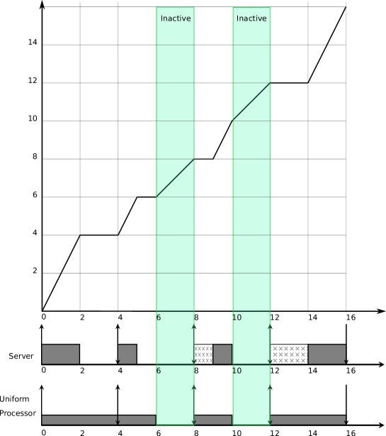
Figure 3: Virtual-time evolution compared to cumulative execution time for an example task scheduled by a server with $Q_{i}=2$ and $P_{i}=4$.

The equivalence between server and uniform processor can be expressed in terms of workload.

Lemma 2.

Let $I_{i}$ be the set of jobs generated by server $S_{i}$; let $\pi^{\prime}$ be the shared identical multiprocessor platform, and let $\pi_{i}$ the uniform processor of speed $U_{i}$. The following relation holds:

$$\forall t,W(EDF,\pi^{\prime},I_{i},t)=W(A,\pi_{i},I_{i},V_{i}(t))$$ (16)

Proof.

It follows directly from the definition of virtual time and the description of the server states in Section 4.1. ∎

Lemma 3.

When a server becomes Inactive, all jobs have completed both in $\pi^{\prime}$ and in $\pi$.

Proof.

It follows directly from Lemma 2. ∎

Therefore, $\pi_{i}$ remains idle until the time when a new job of task $\tau_{i}$ is activated. Let $t_{1}$ denote an instant in which the server (and the corresponding uniform processor) becomes Inactive, and let $t_{2}$ the subsequent instant when $S_{i}$ becomes active again. Since the server is idle, it does not consume any bandwidth so we can reclaim it and donate to another server. However, at time $t_{1}$ we do not know yet when in the future the next job will be activated, so we have to be careful in donating such extra bandwidth.

We divide the interval $[t_{1},t_{2}]$ in a sequence of sub-intervals of infinitesimally small length $\delta$: $\{[t_{1},t_{1}+\delta),[t_{1}+\delta,t_{1}+2\delta),[t_{1}+2\delta,t_{1}+3\delta),\ldots,[t_{2}-\delta,t_{2}]\}$. As time passes, we donate the infinitesimal $\delta U_{i}$ to the needing server. In this way, we can stop as soon as the new job is activated without consuming its reserved budget. To model this donation, we introduce the concept of micro-jobs.

Each such sub-interval represents the arrival time and the absolute deadline of a set of micro-jobs produced by the inactive server. More specifically, for sub-interval $[t,t+\delta)$ we produce $m$ micro-jobs, each one with arrival time at $t$ and absolute deadline at $t+\delta$, and execution time equal to $\frac{U_{i}\delta}{m}$ so that their cumulative execution time is $U_{i}\delta$.

It is easy to see that, if we introduce such micro-jobs on the corresponding dedicated uniform processor, they will all complete before their deadline. Also, the shape of the virtual time will not change. To better understand how it works, consider again the example in Figure 3: in the coloured intervals the server is inactive, and the dedicated processor is idle. In these intervals, we introduce a sequence of micro-jobs, whose cumulative utilisation is equal to $U_{i}$. Clearly, since the uniform processor is idle, it could run all these micro-jobs, and each one would complete before the deadline. Therefore, the workload executed by $\pi_{i}$ by time $t$, including the normal server jobs and all the micro-jobs is always exactly equal to $U_{i}t$. In other words, the micro-jobs are used to fill the idle times that are produced on the uniform processor by the fact that a job terminates earlier than expected. We can repeat this reasoning for every Inactive server (uniform processor, respectively). We have at each instant $m$ micro-jobs for each inactive server, and the cumulative execution time of all the micro-jobs produced by all servers is $\delta U_{\mathsf{inact}}$.

Under G-EDF, these micro-jobs have maximum priority, since their relative deadlines are of infinitesimal length. We have at most $m$ micro-jobs active at every instant, so they execute on every processor for a length of $\delta U_{\mathsf{inact}}$, then they suspend themselves until the next activation at time $t+\delta$. Thus, in an interval of length $\delta$, the $m$ earliest deadline “normal servers” will execute consuming their budget for only $(1-U_{\mathsf{inact}}/m)\delta$, whereas they can execute without consuming their budget (which is accounted for by the micro-jobs) for the remaining $\delta U_{\mathsf{inact}}/m$.

With these observation in mind, we can now proceed to prove the main theorem.

Theorem 4.

If Equation (7) holds, then all jobs produced by all servers under parallel reclaiming will meet their scheduling deadlines.

Proof.

Equation (7) is still respected after adding the micro-jobs (the utilisation of the servers has not changed), therefore Lemma 1 and Theorem 3 are still valid and the new collection of jobs, including the micro-jobs, is schedulable by EDF on the identical multiprocessor platform.

Observe that we can take any small $\delta>0$; hence the $m$ micro-jobs that are active at time $t$ have the highest priority in the identical multiprocessor platform: they execute immediately after their activation for an interval of time equal to $\delta U_{\mathsf{inact}}/m$. Therefore, the executing servers at time $t$ can execute for $\delta U_{i}/m$ without consuming their budget, and for $\delta(1-U_{j}/m)$ consuming their budget. In any case, a server must always consume all its budget within a period $P_{i}$, so the budget decreasing rate of a server cannot be less than $U_{i}$. Therefore, the budget of the servers can be updated in Equation (11), without compromising the schedulability of the servers. ∎

Unfortunately, parallel reclaiming does not work for the BCL test. The reason is that, by dividing all spare bandwidth in parallel pieces, the interference caused to a server may increase too much.

6.2 Proof for sequential reclaiming

The proof of correctness of the sequential reclaiming rule for the GFB test is similar to the proof presented in the previous section: it suffices to create one single micro-job for each reclaiming server. In particular, every Inactive server in interval $[t,t+\delta]$ generates one single micro-job with budget $\delta U_{i}$. Under G-EDF this micro-job will execute with the highest priority on any processor, so we fix it on one specific processor. The proof follows in the same way as the proof of Theorem 4.

Before proceeding with the proof for BCL, we need to discuss the maximum workload $\hat{W}_{i,k}$ for a server $S_{i}$ in the problem window. Moreover, we would like to differentiate two cases.

1. Periodic servers that are always periodically activated by its served tasks.

2. Servers that may be activated aperiodically.

For case (1), it is easy to see that, even with bandwidth reclaiming, the worst-case workload of a server $S_{i}$ in the problem window is realised as in the scenario depicted in Figure 2. This can be checked such that by violating any condition as in Figure 2, the workload will not increase. The scenario is the following:

• Absolute deadline of the last job of $S_{i}$ in the problem window is coincident with $b$.

• All server jobs of $S_{i}$ are periodically released according to the server period $P_{i}$.

• The carry-in server job (i.e., the first job in the problem window) executes as late as possible and finishes exactly at its absolute deadline.

However, when it comes to case (2) such that servers in the system admit aperiodic activation, the scenario in Figure 2 may not correspond to the maximum workload. We provide here a sketch of the reasoning.

Let define $\Delta=(P_{k}\mbox{ mod }P_{i})$ and suppose $\Delta>Q_{i}$. This means that we can anticipate (move to the left) the chain of arrivals in Figure 2 as much as $(\Delta-Q_{i})$ time units without reducing the workload. Moreover, if a server allows aperiodic activation, then from time $b-(\Delta-Q_{i})$ to time $b$, server $S_{i}$ will generate the same micro-jobs as in the proof of Theorem 4, which can at most contribute $(\Delta-Q_{i})U_{i}$ to the workload . In the end, for aperiodic servers with bandwidth reclaiming we formulate $S_{i}$’s workload by Equation (9). More specifically, comparing Equation (8) and (9), the additional term $(\Delta-Q_{i})$ can be regarded as the maximum delay a server job of $S_{i}$ within the problem window can experience such that $S_{i}$’s workload keeps monotonically increasing.

We now prove that, by admitting a server using the test of Equation (10) and then performing sequential reclaiming, no server job misses its deadline.

Theorem 5.

Equation (10) still holds for a set of servers with sequential reclaiming.

Proof.

This proof will deal with the general case and servers may admit aperiodic activations.

We first prove that the formulation in Equation (9) for $\hat{W}_{i,k}$ is indeed the maximum workload. And for simplicity, let us assume that $\Delta>Q_{i}$ (if $\Delta\leq Q_{i}$ the reasoning is the same).

We define $\phi$ to represent the amount of carry-in workload from $S_{i}$, that is, $\phi=\min\{Q_{i},P_{k}\mbox{ mod }P_{i}\}$. And $W^{\prime}$ denotes the amount of workload from execution of non-carry-in jobs of $S_{i}$ within the problem window such that these jobs have absolute deadlines no later than time point $b$; let say there are $n^{\prime}$ such jobs, that is, $n^{\prime}=\lfloor\frac{P_{k}}{P_{i}}\rfloor$. Then, the maximum workload by micro-jobs from $S_{i}$ (that is, workload caused by donating bandwidth to other servers’ execution) would be $(n^{\prime}P_{i}-\frac{W^{\prime}}{U_{i}})U_{i}+(\Delta-Q_{i})U_{i}=n^{\prime}P_{i}U_{i}-W^{\prime}+(\Delta-Q_{i})U_{i}$. Remind that $(\Delta-Q_{i})U_{i}$ is the part of workload resulted from $S_{i}$’s aperiodic behaviour.

The total workload due to $S_{i}$ within the problem window is $\phi+W^{\prime}+(n^{\prime}P_{i}U_{i}-W^{\prime})+(\Delta-Q_{i})U_{i}=\phi+n^{\prime}Q_{i}+(\Delta-Q_{i})U_{i}=\hat{W}_{i,k}$. As we can see, the interference upon the target job due to workload from $S_{i}$ can be upper bounded by $\hat{W}_{i,k}$.

On the other side, a server can donate its budget only when it is inactive and at any time its budget can be used by at most one executing server (according to the sequential reclaiming rule). That is, the execution of $S_{i}$ and its budget donation must be in a sequential way. Thus, if $S_{k}$ is schedulable, the interference due to $S_{i}$ within the problem window can still be upper bounded by $(P_{k}-Q_{k})$.

In the end, Equation (10) still holds if sequential reclaiming is applied. ∎

7 Conclusions

In this report, we proposed two different reclaiming mechanisms for real-time tasks scheduled by G-EDF on multiprocessor platforms, named parallel and sequential reclaiming. In the future we plan to conduct further investigations comparing the two strategies, and to use more advanced admission tests.

References

- [1] L. Abeni and G. Buttazzo. Integrating multimedia applications in hard real-time systems. In Real-Time Systems Symposium, 1998. Proceedings., The 19th IEEE, pages 4–13. IEEE, 1998.
- [2] L. Abeni, J. Lelli, C. Scordino, and L. Palopoli. Greedy CPU reclaiming for SCHED_DEADLINE. In Proceedings of the Real-Time Linux Workshop (RTLWS), Dusseldorf, Germany, October 2014.
- [3] S. K. Baruah, J. Goossens, and G. Lipari. Implementing constant-bandwidth servers upon multiprocessor platform. In IEEE Real Time Technology and Applications Symposium, pages 154–163, 2002.
- [4] S. K. Baruah, L. E. Rosier, and R. R. Howell. Algorithms and complexity concerning the preemptive scheduling of periodic, real-time tasks on one processor. Real-time systems, 2(4):301–324, 1990.
- [5] G. Bernat, I. Broster, and A. Burns. Rewriting history to exploit gain time. In Real-Time Systems Symposium, 2004. Proceedings. 25th IEEE International, pages 328–335. IEEE, 2004.
- [6] M. Bertogna and S. Baruah. Tests for global EDF schedulability analysis. Journal of Systems Architecture, 57(5):487–497, 2011. Special Issue on Multiprocessor Real-time Scheduling.
- [7] M. Bertogna, M. Cirinei, and G. Lipari. Improved schedulability analysis of EDF on multiprocessor platforms. In Proc. 17th Euromicro Conf. Real-Time Systems (ECRTS 2005), pages 209–218. Published by the IEEE Computer Society, 2005.
- [8] B. B. Brandenburg and J. H. Anderson. Integrating hard/soft real-time tasks and best-effort jobs on multiprocessors. In Proceedings of the Euromicro Conference on Real-Time Systems, pages 61–70, Pisa, July 2007.
- [9] M. Caccamo, G. Buttazzo, and L. Sha. Capacity sharing for overrun control. In Real-Time Systems Symposium, 2000. Proceedings. The 21st IEEE, pages 295–304. IEEE, 2000.
- [10] J. Goossens, S. Funk, and S. Baruah. Priority-driven scheduling of periodic task systems on multiprocessors. Real-time systems, 25(2-3):187–205, 2003.
- [11] J. Lelli, G. Lipari, D. Faggioli, and T. Cucinotta. An efficient and scalable implementation of global EDF in Linux. In Proceedings of the international workshop on operating systems platforms for embedded real-time applications (OSPERT), 2011.
- [12] J. Lelli, C. Scordino, L. Abeni, and D. Faggioli. Deadline scheduling in the Linux kernel. Software: Practice and Experience, pages n/a–n/a, 2015.
- [13] C. Lin and S. Brandt. Improving soft real-time performance through better slack reclaiming. In Real-Time Systems Symposium, 2005. RTSS 2005. 26th IEEE International, pages 12–pp. IEEE, 2005.
- [14] G. Lipari. Resource reservation in real-time systems. PhD thesis, PhD thesis, Scuola Superiore S. Anna, Pisa, Italy, 2000.
- [15] G. Lipari and S. K. Baruah. Greedy reclamation of unused bandwidth in constant-bandwidth servers. In Proc. 12th Euromicro Conf. Real-Time Systems Euromicro RTS 2000, pages 193–200. IEEE, IEEE Computer Society, 2000.
- [16] L. Nogueira and L. M. Pinho. Capacity sharing and stealing in dynamic server-based real-time systems. In Parallel and Distributed Processing Symposium, 2007. IPDPS 2007. IEEE International, pages 1–8. IEEE, 2007.
- [17] R. Pellizzoni and M. Caccamo. M-cash: A real-time resource reclaiming algorithm for multiprocessor platforms. Real-Time Systems, 40(1):117–147, 2008.
- [18] R. Rajkumar, K. Juvva, A. Molano, and S. Oikawa. Resource kernels: A resource-centric approach to real-time and multimedia systems. In Photonics West’98 Electronic Imaging, pages 150–164. International Society for Optics and Photonics, 1997.